Midterm Supply Chain Planning under Uncertainty: A Multiobjective ChanceConstrained Programming Framework†

Kishalay Mitra,‡ Ravindra D. Gudi,*,§ Sachin C. Patwardhan,§ and Gautam Sardar‡

Tata Consultancy SerVices, 1 Mangaldas Road, Pune 411001, India, and Indian Institute of Technology,Bombay, Powai, Mumbai 400076, India

Uncertainty issues associated with a multisite, multiproduct supply chain planning problem has been analyzedin this paper, using the chance constrained programming (CCP) approach. In the literature, such problemshave been addressed using the scenario-based two-stage stochastic programming approach. Although thisapproach has merits, in terms of decomposition, the computational complexity, even for small-size planningproblems, is generally quite large, leading to either huge time consumption in solving the problem or aninability to solve big instances of problems under a standard solver environment. To make the aforementionedlacunea of two-stage stochastic programming more tractable, the problems under uncertainty have been recastin this paper in a CCP framework that uses a more suitable representation of uncertainty. Addressing uncertaintyissues in product demands and machine uptime, using the CCP approach, leads to the evaluation ofmultiobjective tradeoffs that are analyzed here in the Pareto sense, and the ε-constraint approach is used togenerate those Pareto optimal (PO) points. Different aspects of uncertainty issues are analyzed in detail bytaking a few PO points among the total set of PO solutions found for this problem. It is seen that this CCP-based approach is quite generic, relatively simple to use and can be adapted for bigger size planning problems,as the equivalent deterministic problem does not blow up in size with the CCP approach. We demonstrate theanalysis on a relatively moderate size midterm planning problem taken from published work [McDonald,C. M.; Karimi, I. A. Ind. Eng. Chem. Res. 1997, 36, 2691] and discuss various aspects of uncertainty in thecontext of this problem.

Introduction

The primary objective of any supply chain planning iseffective coordination and integration of the key businessactivities undertaken by an enterprise, starting from the procure-ment of raw materials to the distribution of the final productsto the customers. The competitive pressures of the globaleconomy motivate manufacturing and service enterprises tofocus on supply chain planning on a priority basis.1 In thevolatile market situations where enterprises must meet customersatisfaction under changing market conditions, it is more realisticto consider the effect of uncertainties on supply chain planning,to minimize their impact; deterministic models are unable tocapture the demands and tradeoff between various cost com-ponents such as inventory costs and demand satisfactionrealistically in the presence of uncertainty. In practice, the sourceof uncertainties can be quite varied, beginning with the productdemand, raw material supply, processing rates, unit costsprocessing variations, equipment uptimes, canceled orders, etc.that may occur over different time horizons considered forplanning: strategic (i.e., long-term), tactical (mid-term), andoperational (short-term). Tactical planning is a link betweenstrategic level planning (related with the design of supply chainsthat affects the long-term performance of the system, e.g.,decisions of investments for capacity expansion, etc.) andoperational level planning (associated with the day-to-dayactivities relating the exact sequencing of the manufacturingtasks, considering resource and time constraints) where, given

a fixed supply chain topology, the best coordination betweenvarious supply chain entities (such as raw material suppliers,production units, warehouses, retailers, and customers) isachieved over an intermediate time frame.1

The representation of the uncertain parameters is the keydistinguishing feature among various prevailing methods ofhandling uncertainties. Stochastic programming (programmingwith recourse),2–11 fuzzy mathematical programming (flexibleand possibilistic programming),12–18 and probabilistic pro-gramming19–24 are the three most popular approaches ofhandling uncertainties.25

Programming with recourse,2–11under stochastic program-ming, uses the standard two-stage approach, where the decisionvariables are partitioned into two sets. The first-stage variablesare to be decided before the realization of uncertain parameters(“here and now” decisions), whereas the second-stage variablesare chosen as a corrective measure against any infeasibilityarising due to a particular realization of uncertainty. Theobjective here is to choose the first-stage variables in such away that the sum of the first-stage costs and the expected valueof the random second-stage costs is minimized. The concept ofrecourse has been applied to linear, integer, and nonlinearprogramming problems.19 The main challenge in solving thetwo-stage stochastic problem is the calculation of expectationterm for the inner recourse problem. Uncertainty can beexpressed in two different ways for the two-stage programs.The scenario-based approach26–28 represents a random param-eter by forecasting all its future outcomes. This method has amajor drawback, in that it leads to an exponential increase inproblem size with an increase in the number of scenarios to beanalyzed, even for a smaller problem. With increasing problemsize, the problem becomes completely intractable by standardoptimization solvers. To overcome this difficulty, continuousprobability distributions (distribution-based approach4,29,30) for

* To whom correspondence should be addressed. Tel.: 91-22-25767204. Fax: 91-22-2572-6895. E-mail address: ravigudi@che.iitb.ac.in.

† A condensed version of this manuscript was accepted for presenta-tion to the 17th IFAC World Congress (2008).

‡ Tata Consultancy Services.§ Indian Institute of Technology.

Ind. Eng. Chem. Res. 2008, 47, 5501–5511 5501

10.1021/ie0710364 CCC: $40.75 2008 American Chemical SocietyPublished on Web 07/09/2008

random parameters are used; this makes the problem nonlinearbut brings the advantage of a substantial decrease in the problemsize. Calculation of the inner recourse expectation term for ascenario-based approach associates a second-stage variable foreach of the scenarios and solves a large-scale extensiveformulation, using either the Dantzig-Wolfe approach31 or theBenders decomposition-based approach.32 For continuous prob-ability distributions, this challenge is primarily resolved throughthe discretization of the probability space for approximating themultivariate probability integrals. Various sampling techniquessuch as Monte Carlo, Gaussian quadrature, Latin hypercube,Shifted Hammerslay Sequence Sampling,33 etc. are used for thispurpose. The disadvantage of these methods is the sharp increasein computational requirements with the increase in the numberof uncertain parameters.

Similar to stochastic programming, fuzzy mathematicalprogramming12–18 has also been used to address optimizationproblems under uncertainty, where uncertain parameters aretreated as fuzzy numbers and constraints are treated as fuzzysets.13,14 A small extent of constraint violation is allowed andthe degree of satisfaction of a constraint is defined in terms ofthe membership function of the constraint. Objective functionsare also considered as constraints here, with the upper and lowerbound for these constraints defining the expectation of thedecision maker. Flexible programming12–16 and possibilisticprogramming17,18 are alternate representation and solutionmethods that fall under the category of fuzzy mathematicalprogramming. Flexible programming12–16 is concerned with theuncertainties that occur with the terms independent of associationwiththedecisionvariable,whereasthepossibilisticprogramming17,18

is concerned about the uncertainties in the decision variablecoefficients as well. With the linear membership function (whichoften provides the same quality final solutions, in comparsionto their nonlinear counterpart) defining the fuzziness of extentof satisfying a constraint, a flexible programming problem canbe derived as a classical linear program (or mixed integer linearprogram) and solved using standard linear programming (LP)methods.12–18,25 Similarly, possibilistic programming problemcan be derived as a classical nonlinear program (or mixed-integernonlinear program) and solved using various nonlinear program-ming (NLP) methods. The main drawback in this approach,however, is that the user must define the fuzziness, which maynot always be very clearly known.

The recourse-based approach to stochastic programmingrequires the decision maker to assign a cost to recourse activitiesthat are taken to ensure feasibility of the second-stage problem.However, these compensating second-stage actions often eitherlead to impracticality (actions difficult to execute practically)or difficulty in specifying the cost associated with the decision.In such circumstances, emphasis is shifted toward the reliabilityof a system by requiring a decision to be feasible with highprobability. In the probabilistic programming19–25 or chance-constrained programming (CCP) approach, the focus is on thesystem’s ability to meet feasibility in an uncertain environment.This reliability is expressed as a minimum requirement on theprobability of satisfying constraints. This stochastic formulationof CCP leads to an equivalent deterministic formulation, andthe resultant problem can be solved. The main advantage ofthis technique is the emergence of the relatively small deter-ministic equivalent problem (LP/NLP), even in the presence ofa large number of uncertain parameters that can be solved quiteeasily to obtain the optimal operating conditions under uncertainsituations.19–24 Applications of CCP for solving problems underuncertainty in process system and engineering literature have

been relatively fewer, when compared with two-stage stochasticprogramming methods, except for a few works (e.g., optimalmolecular design21 and planning for biopharmaceutical produc-tions23). The work on molecular design proposed an exhaustiveand systematic approach to assess tradeoffs among performanceobjectives (e.g., property matching), probabilities of meetingthe objectives, and chances of satisfying design specificationsto guide the optimal molecular design procedure in the presenceof property prediction uncertainty (imprecision). On the otherhand, the example of midterm biopharmaceutical batch produc-tion planning23 showcased the edge of CCP over the two-stageprogramming, accompanied by an iterative construction algo-rithm, in terms of solution quality (profitability and capacityutilization), as well as execution time, while solving formaximization of profit function in the presence of uncertaintyin fermentation titers. However, the field of supply chainplanning and logistics poses many other challenges over andabove the scope of batch production planning and may have toconsider manufacturing and logistics constraints related toproduction, as well as transportation among various sites andadditional uncertainty, in terms of product demand, machineuptime, safety target inventory, and cost coefficients. Moreover,multiobjective tradeoff analysis is desirable in a supply chaincontext from the viewpoints of different priorities or precedenceordering of different objectives in the supply chain planningproblem, and it would provide the designer a suitable basis fordecision making.

Therefore, in this paper, we explore the merits of CCP towardaddressing the uncertainty issues of product demand andmachine uptime associated with a multiobjective, multisite,multiproduct supply chain tactical planning problem. In theliterature, these problems have been addressed using the two-stage stochastic programming approach.34,35 Gupta and Ma-ranas35 solved the supply chain planning problem using a two-stage stochastic programming approach where they replaced thecomputationally expensive second-stage expectation term by ananalytical expression. To derive this analytical expression, theydivided the entire demand space into three regimes of uncertaindemand (low, intermediate, and high) and used some fixedtransition rules to derive supply policies for assigning productsto the market for each of the demand regimes by artificiallydividing the production sites into two parts: internally sufficientand internally deficient. Finally, a demand satisfaction equationwas defined and the uncertainty analysis of only this equationwas done using CCP. In our work, we propose to analyze issuesrelated to all the uncertain parameters using CCP, to evolve asuitable policy that effectively responds to the uncertain demandsof the market, as well as machine uptime. This latter approachobviates the need to make any assumptions related to thedemands and production sites, and it also does not require thedevelopment of any transition rules. Another novelty of ourapproach presented here is in the analysis of tradeoffs in amultiobjective pareto sense, which provides the basis fordecision making for a supply chain planner, under uncertainconditions. While the two-stage stochastic programming ap-proach has merits in terms of decomposition, the associatedcomputational complexity for a scenario-based approach34 orthe theoretical development of the optimization problem for-mulation for a distribution-based approach,34,35 even for smallsize planning problem, is large. This problem is overcome inour paper by adopting the CCP approach for solving the mid-term planning problem. The mid-term planning model ofMcDonald and Karimi36 forms the basis of this work on whichvarious impacts of uncertainty have been analyzed.

5502 Ind. Eng. Chem. Res., Vol. 47, No. 15, 2008

The remainder of the paper is organized as follows. In thenext section, a brief overview of CCP is presented. The nextsection on optimization problem formulation contains thedescription on the planning problem of the McDonald andKarimi,36 along with their adaptation into the CCP framework.The results of planning under uncertainty are presented in theResults and Discussion section for the first case study of thework of McDonald and Karimi.36 Finally, the work is sum-marized and concluding remarks are provided.

Chance Constrained Programming

A brief overview of chance constrained programming (CCP)is presented in the following section. Interested readers arereferred to various literature19–25 for a more detailed description.In CCP, constraints that are associated with random parametersare expressed in terms of a certain probability of getting satisfied.In this framework, a standard optimization formulation withuncertainty parameter �,

Min{ f (x)|h(x, �)g 0} (1)

can be expressed as

Min{ f (x)|P(hk(x, �)g 0)g p} (k) 1, ..., u) (2)

where f(x) is the objective function, x the set of continuousdecision variables, � the set of random parameters, P theprobability measure of the given probability space of theuncertain parameter, and p ∈ (0,1] the probability level withwhich each of the u constraints hk(x, �) g 0 of the entireconstraint set hk(x, �) g 0 must be satisfied. The higher thevalue of p, the more reliable the system, with respect to theuncertain parameter. On the other hand, the set of feasible xvalue shrinks more and more as the value of p approaches unity.Based on the requirements of several constraints getting satisfiedeither individually or together, the methodology is calledindividual or joint chance constrained programming, respec-tively. These two different concepts can be represented as eqs2 and 3, respectively.

Min{f(x)|P[(hk(x, �)g 0) (k) 1, ..., u) ]g p} (3)

It is seen that feasibility in the joint chance constrained caseinvolves feasibility in the individual chance constrained case,but the reverse is not true. In the joint chance constrained case,the deterministic equivalent form incorporates the quantile formon the multivariate probability distribution, considering all therandom parameters under consideration. Passing from joint toindividual chance constraints may appear as a complication, inthat it transforms a single inequality into a multiple number (u)of inequalities. Because the numerical treatment of probabilityfunctions that involve high dimensional random vectors is muchmore difficult than in one dimension, the increase in the numberof inequalities is more than compensated by a much simplerimplementation. Unlike the two-stage stochastic programmingapproach, the advantage of these methods is that they arerelatively easy to formulate and the problem size of the resultantdeterministic equivalent does not blow up, even for large numberof random parameters.

Assuming (i) a normal distribution for the random parameter� and (ii) that random parameters are separable from the decisionvariables, the constraints in eq 2 can be transformed to anequivalent deterministic form:

P(hk(x, �)g 0)g p S P(h̃k(x)g �k)g p

S P(h̃k(x)g �k)g p(4)

where �k is the random parameter associated with the kthconstraint; �jk and σ�k are the mean and standard deviation valuesof the corresponding random parameters; and qp is the p-quantileof the standard normal distribution with zero mean and unitstandard deviation (e.g., 97% probability corresponds to qp )q0.97 ) 2.0). If the random parameters are not separable, similartreatment must be done with the decision variable terms in eq4. The second term in the last equivalence form of eq 4 (quantilevalue multiplied by standard deviation) corrects the nominalrequirement �jk and provides robustness of the generated optimaloperating conditions, under uncertain situations. In this case,the uncertainty terms are not separable from the decisionvariables, based on whether the uncertain terms are independentor dependent on each other, the corresponding mean andvariance terms are incorporated into the equation in the samefashion, and the deterministic equivalent form is derived. Thisdeterministic equivalent generally becomes nonlinear as thecomputation of mean and variance of coefficients of decisionvariable leads to nonlinearity, in terms of decision variables.

For an efficient treatment of probabilistic constraints, it isvery crucial to have some insight into their analytical, geometric,and topological structure. Most results in this direction areconcerned with the convexity issues of the resultant deterministicproblem in the CCP approach. It is known that, if the individualconstraints of the constraint set h(x, �) is convex and � has sucha probability density that the logarithm of which is concave,then P(h(x, �) g 0) is concave and the corresponding proba-bilistic constraint may be convex.19,20 Otherwise, the resultantdeterministic form may not be convex and issues related to thisshould be treated either with proper convexification approachesor with various global optimization techniques, conventionalor evolutionary methods, for handling the resultant NLPproblems.

Modeling Supply Chain Uncertainty Under the CCPFramework

There are several entities in the supply chain, namely, rawmaterial supplier, production unit, retailer, and customer. Giventhe topology of these entities, the purpose of the planning modelis to determine (i) the amount to be procured as raw material atproduction sites; (ii) the amount to be produced at the productionunits; (iii) the amount to be shipped from production unit tosuppliers, suppliers to markets, or among various productionunits (for the production of interdependent products); (iv) theamount of inventory to be kept at various locations (safety stock)to meet the stochastic demand prevailing in the market for theoptimal operation of the supply chain over a relatively moderatetime period (1-2 years). The generic (mixed-integer linearprogramming, MILP) mid-term planning model of McDonaldand Karimi36 is adapted here for the discussion related to thedemand uncertainty. We present the model as follows:

Minimize Cost:

Cost) ∑i,j,s,t

νi,j,sPi,j,s,t +∑i,s,t

pi,sCi,s,t +∑i,s,t

hi,s,tIi,s,t +

∑i,s,c,t

ts,cSi,s,c,t + ∑i,s,s′,t

ts,s′σi,s,s′,t +∑i,s,t

�i,sIi,s,t∆ +∑

i,c,t

µi,cIi,c,t- (5)

Cost) ∑f,j,s,t

FCf,j,s,tYf,j,s,t + ∑i,j,s,t

νi,j,sPi,j,s,t +∑i,s,t

pi,sCi,s,t +

∑i,s,t

hi,s,tIi,s,t + ∑i,s,c,t

ts,cSi,s,c,t +

∑i,s,s′,t

ts,s′σi,s,s′,t +∑i,s,t

�i,sIi,s,t∆ +∑

i,c,t

µi,cIi,c,t- (6)

Ind. Eng. Chem. Res., Vol. 47, No. 15, 2008 5503

Manufacturing Constraints:

Pi,j,s,t )Ri,j,s,t RLi,j,s,t ∀ i ∈ I \ IRM (7)

∑i

RLi,j,s,t -Hj,s,te 0 (8)

∑f

RLf,j,s,t -Hj,s,te 0 (9)

RLf,j,s,t ) ∑i∈ Φi,f

RLi,j,s,t (10)

Ci,s,t ) ∑i′��i′,i,s*0

�i′,i,s∑j

Pi′,j,s,t ∀ i) I \ I FP (11)

Ci,s,t )∑s′

σi,s′,s,t ∀ i) I IP (12)

Supply Chain Constraints:

Ii,s,t ) Ii,s,t-1 +∑j

Pi,j,s,t -∑s′

σi,s′,s,t -∑c

Si,s,ct ∀ i ∈ I \ I RM

(13)

Ii,c,t- g Ii,c,t-1

- + di,c,t -∑s

Si,s,c,t ∀ i ∈ I FP (14)

∑s,t′et

Si,s,c,t′e∑t′et

di,c,t′ ∀ t ∈ T (15)

Ii,s,t∆ g Ii,s,t

L - Ii,s,t ∀ i ∈ I FP (16)

Lower Bound Constraints:

Pi,j,s,t, RLi,j,s,t, RLf,j,s,t, Ci,s,t, Si,s,c,t, Ii,s,t, Ii,c,t- , σi,s,s′,t, Ii,s,t

∆ g 0

(17)

Yf,j,s,t ∈ {0, 1} (18)

Upper Bound Constraints:

Pi,j,s,teRi,j,s,t Hj,s,t (19)

RLi,j,s,t -Hj,s,te 0 (20)

RLf,j,s,t -Hj,s,tYf,j,s,te 0 (21)

RLf,j,s,t -MRLf,j,s,tYf,j,s,tg 0 (22)

Ii,s,t∆ e Ii,s,t

L (23)

Si,s,c,te∑t′et

di,c,t′ (24)

Ii,c,t- e∑

t′et

di,c,t′ (25)

where Pi,j,s,t, RLi,j,s,t, RLf,j,s,t,Ci,s,t, Si,s,c,t, Ii,s,t, Ii,c,t- , σi,s,s′,t,Ii,s,t

∆

represents the production, run length for each product, run lengthfor each product family, consumption, supply to the market,inventory at production site, missing demand at market,intermediate product, inventory below safety level for producti or family f of several products to be produced at facility j atsite s or customer c or market m at time period t, respectively.Here, Yf,j,s,t represents the binary variable used to decide whethera product family f will be produced at machine j, site s, andtime period t. A few other important parameters are demand(di,c,t), machine uptime (Hj,s,t), minimum run length for theproduct family f (MRLf,j,s,t), safety stock target for product (Ii,s,t

L ),and effective rate of production (Ri,j,s,t), whereas various unit-cost parameters are inventory holding cost (hi,s,t), revenue (µi,c),raw material price (pi,s), penalty for dipping below safety level

(�i,s), fixed production cost (FCf,j,s,t), and variable productioncost (νi,j,s) and transportation costs (ts,s′,ts,c).

The set of products in the system is denoted by the index setI ≡ {i}. This set can be classified into three categories: (1) rawmaterials (IRM), (2) intermediate products (IIP), and (3) finishedproducts (IFP), so that I ) {IRM∪IIP∪IFP}. An intermediateproduct can also belong to the set of finished products. The setof machines is denoted as J ≡ {j}, and the set facilities wherethese machines are located are denoted as S ≡ {s}. The set ofcustomers is denoted as C ≡ {c}, whereas the set of time periodis denoted as T ≡ {t}. F ≡ {f} represents the set of families,and Φi,f is defined as the cross-set indicating that product i is amember of family f. We refer the readers to the work ofMcDonald and Karimi36 for further details regarding themodeling part, because further details are not provided here (forthe sake of brevity).

In the aforementioned planning model, uncertain demandsappear as terms independent of the decision variables, and,therefore, eqs 14, 15, 24, and 25 are modified accordingly (seeeqs 26–29). All four demand-related constraints are solved withprobability p, and, therefore, a corresponding quantile value ofqd is used, assuming a normal distribution for all productdemands. Equations that have uncertain demand terms aremodified to the following form, where different dji,c,t values arethe nominal values of different products i and σdi,c,t are theircorresponding standard deviation figures. Similarly, the equa-tions concerning uncertainty that is related to machine uptime(eqs 8, 9, 19, 20, 21) are also accordingly modified into eqs30–34, where Hj j,s,t, σmj,s,t, and qm are their corresponding nominal,standard deviation, and quantile value figures, assuming anormal distribution for this case as well. All the randomvariables (e.g., product demand as well as machine uptime) areassumed to be statistically independent.

Ii,c,t- g Ii,c,t-1

- + (di,c,t + qdσdi,c,t)-∑

s

Si,s,c,t ∀ i ∈ I FP

(26)

∑s,t′et

Si,s,c,t′e∑t′et

(di,c,t + qdσdi,c,t) ∀ t ∈ T (27)

Si,s,c,te∑t′et

(di,c,t + qdσdi,c,t) (28)

Ii,c,t- e∑

t′et

(di,c,t + qdσdi,c,t) (29)

∑i

RLi,j,s,te (Hj,s,t - qmσmj,s,t) (30)

∑f

RLf,j,s,te (Hj,s,t - qmσmj,s,t) (31)

Pi,j,s,teRi,j,s,t(Hj,s,t - qmσmj,s,t) (32)

RLi,j,s,t - (Hj,s,t - qmσmj,s,t)e 0 (33)

RLf,j,s,t - (Hj,s,t - qmσmj,s,t)Yf,j,s,te 0 (34)

Maximize Reliability:

ql (l) d or m) (35)

Because the reliability of the model (eq 35) has an inherentPareto tradeoff with the total cost of the model, we finally obtainthe formulation for the biobjective optimization using theplanning model. Equations 5–35 (except eqs 8, 9, 14, 15, 19,20, 21, 24, and 25) form the complete set of equations describing

5504 Ind. Eng. Chem. Res., Vol. 47, No. 15, 2008

the multiobjective planning model under demand as well asmachine uptime uncertainty, which is solved here using theε-constraint approach.38–40 Some other popular approaches forhandling multiobjective optimization problems are the weightedsum approach and the goal programming method.38–40 In theε-constraint approach, all objectives except one are convertedto constraints and different ε values are associated with each ofthese constraints, taken one at a time, and the resultant singleobjective optimization problem is solved to find Pareto optimal(PO) solutions. Different PO solutions correspond to thedifferent sets of ε values attached with each of the constraints.For example, in the case of our problem, where we intend tominimize cost and maximize reliability simultaneously, theequivalent single objective optimization problem through theε-constraint approach becomes

Min Cost s.t. qlg εq Other relevant constraints(36)

As cost increases (or decreases) with an increase (or decrease)in ql, minimizing cost with a greater than equal to constrainton ql will provide a set of trade-off PO points between themfor different values for εq.

In the case of the weighted sum approach, a weight is assignedwith each objective and the different PO points are generatedusing different combinations of the weight vector (w ) [w1,w2]), given w1 + w2 ) 1. In the goal programming method,41–45

we convert the objectives given in any of the following goals(t is the target of the goal):46

(1) Less than equal to, type (f(x) e t)(2) Greater than equal to, type (f(x) g t)(3) Equal to, type (f(x) ) t)(4) Within a range, type (f(x) ∈ [tl, tu])To achieve the aforementioned goals, two non-negative

variables (deviation from the target), n and p, are introduced.This transforms the “less than equal to” goal into f(x) - p e tand the “greater than equal to” goal into f(x) + n g t. Thus,the target of goal programming is to convert each of theobjectives into at least one equality constraint and to minimizethe weighted sum of all deviations. Therefore, the equivalentgoal programming problem becomes

Min w1 × p + w2 × n (37)

s.t. Cost- p)TargetCost

Cost+ n)TargetReliability

n, pg 0Other relevant constraints

and different values of the weight vector (w ) [w1, w2]) canprovide the various points on PO front.

In the absence of any precedence ordering among the differentobjectives, the ε-constraint method is a preferred alternative andhas been chosen in this paper to generate the PO set of solutions.

Considering the complete set of equations for the planningunder demand, as well as machine uptime uncertainty, we seethat all constraints are linear and the assumed probabilitydistribution is a normal distribution; therefore, the problem isconvex19,20 and can be expected to yield globally optimalsolutions. Note that the aforementioned arguments will not holdfor a general case of an MILP.

Results and Discussions

The motivating example considered here is taken from thefirst case study of McDonald and Karimi.36 There are two

production locations (S1 and S2) that have one unit in each ofthem. Each of this production unit has a single raw materialsupplier. Production units S1 and S2 are connected to marketM1 and M2, respectively. There are 34 products that are underconsideration in this supply chain. The unit at location S1manufactures products P1-P23, whereas products P24-P34 aremanufactured at location S2. Products at location S2 areproduced from a set of intermediate products that are producedat location S1, e.g., product P24 is produced from product P1,product P25 is produced from product P4, product P26 isproduced from product P6, and so on, as shown in Figure 1.There are 11 product families (F1-F11) that are composed bylumping the products of the production site S1 (e.g. productsP1, P2, and P3 form product family F1, products P4 and P5form product family F2, and so on, as shown in Figure 1).Market M1 has a set of customers who have demands forproducts P1-P23 and market M2 has customers that hasdemands for products P24-P34. We assume that the demanduncertainty for all 34 products can be reasonably modeled by anormal distribution. Nominal demands for all these productsare taken as the deterministic demand values, given in theoriginal problem for a 1-year planning horizon (with a timeperiod of duration of 1 month; therefore, 12 such time periodsare considered). To see the effect of sudden rise in demand,the demand values for time periods 6 and 12 are changed to300% of the demand values given in the original work, whileall other demand values for the remaining 10 time periods areconsidered to be 20% of the demand values reported in theoriginal problem and the nominal demands for the uncertaincase are updated accordingly. We analyze the effect ofuncertainty for two formulations, viz (i) multiobjective mid-term planning product formulation without any minimum runlength restriction (henceforth called Model 1, consisting of eqs5, 7, 8, 11–13, 16, 17, 19, 20, 23, 26–29, and 35) and (ii)multiobjective mid-term planning product family formulationwith a minimum run length restriction (henceforth called Model2, consisting of eqs 6–13, 16–23, 26–29, and 35). The firstproblem results in an LP formulation, whereas the second

Figure 1. Supply chain topology, as well as product-family distribution,for the motivating example problem.

Ind. Eng. Chem. Res., Vol. 47, No. 15, 2008 5505

problem is an MILP problem. The complete formulation wascoded in the modeling environment of GAMS37 and solvedusing the BDMLP37 solver. A typical optimization run for model1 (LP) includes 4379 single equations and 2723 single variables,and it was solved in an average time of 0.5 CPU s, whereas asimilar formulation in model 2 (MILP) includes 4788 singleequations, 2988 single variables, and 132 binary variables, andwas solved in an average in 300 CPU s (a maximum limit iskept as 5000 nodes to be checked). Model 2 was determined toconverge to 4% of the best possible value, with an averageabsolute gap of 300, spanning over 25 different runs.

Multiobjective Pareto Tradeoff between Reliability andCost. The Pareto optimal (PO) points for models 1 and 2, withdemand variations of 10% and 15% of the nominal values,respectively, are presented in Figure 2. Different instances ofreliability for demand uncertainty model (henceforth called thedemand reliability index (DRI), Dr) were obtained by changingthe quantile value, qd, of the standard normal distribution curveof demands for different products. A Dr value closer to 1represents a demand reliability of 84.1345%; this would implythat the demands would lie within the first quantile 84.1345%of the time and, therefore, inclusion of such a description inthe demand satisfaction constraint would represent the demanduncertainty to the aforementioned extent. Similarly, Dr valuesof 2 and 5 represent demand reliabilities of 97.725% and99.9999%, respectively. On each of these PO fronts, one extremepoint can be interpreted as one that yields the most demand-reliable system (the higher Dr value side, e.g., 6), whereas theother extreme point represents the least expensive solution (thelow Dr value side, e.g., 1). The value of Dr is not restricted toany integer value. A decision maker must make a single choiceamong all PO points as the operating point, based on the demandsatisfaction requirement. As the uncertainty increases, Figure 2shows that the same value of demand reliability (Dr) is obtainedat higher cost; hence, the PO front for the higher standarddeviation case lies above the front, corresponding to therelatively smaller standard deviation case. The PO front of model2 (MILP) also lies marginally above the PO front of model 1,because model 2 (MILP) is a more restrictive case of model 1(LP) and, hence, leads to higher cost. Various cost componentsof the total model cost for model 2 for different values of Dr

are presented in Figure 3. As the total cost increases with anincrease in Dr, the penalty cost for the inability to maintain a

safety level and the cost for missing customer demands alsoincrease proportionately. With an increase in reliability of themodel, the model has a tendency to meet more demands, ifrequired, at the cost of safety stocks, because the unit-cost valueof the product revenue is more than that of the penalty values.Therefore, the safety stocks are allowed to deplete first in thosecases, followed by demand miss, if the productions are at theirrespective full capacities. However, similar trends are notobvious for other cost components in the objective function.

Assessing Uncertainty: Variation in Demand. Here, wefocus on a few points of the model 2 PO front (points A and Bin Figure 2): specifically, we focus on the two points corre-sponding to Dr ) 2, i.e., the points corresponding to the 10%and 15% demand variation cases. These two cases are comparedwith the results of the planning model run in a deterministicfashion for the nominal values of the demands (henceforth calledthe deterministic benchmark case). The demand, production, andinventory storage patterns for product P1 can be seen from theresults presented in Figure 4. As compared to the nominal case,the plan for the uncertainty cases shows a trend of higherproduction to handle uncertainty in future. The starting ofproduction only around the sixth time period can be attributedto the demand until that time period being met by the alreadyexisting initial inventory at the production site. More accumula-tion of inventory for future uncertainty is not visible, becausethere is a cost associated with it. On a relative basis, the unit-cost component of the McDonald and Karimi36 model is definedin such a way that the model gives higher preference formaintaining inventory at the safety level as long as there is nodemand miss and that happens during time periods 6-11. Attime period 12, the model allows its safety level to becomedepleted to meet market demand, because the cost associatedwith a missing demand at market is higher than the inventorycosts. The case is more aggravated when the variance of theproduct uncertainty is higher (15%). Because all of the 34products are to be produced over 12 time periods withinterdependence between various products (with finite produc-tion capacity), a straightforward correlation among the patternsand the variance is not obvious. However, generally, as theuncertainty grows, the equivalent deterministic demand in-creases, leading to higher production rates, in comparison tothe nominal conditions. Similar results for the other 33 productswere generated to verify the aforementioned hypothesis but arenot presented here for the sake of brevity. The nominal casepresented here shows why uncertainty cannot be handled usingthe mean values of the demands and leads to either misses ofpotential opportunity or unnecessary and untimely accumulationof inventory, leading to very high inventory costs. The relativeresults of uncertainty analysis for models 2 and 1 are presentedin Figures 4 and 5, respectively. The significant difference inthese two cases arises because of the absence of the minimumrun length as well as product family constraint in the case ofmodel 1 due to which products are made at all possible timenodes, if required. This ensures that no demand is missed unlessmachines are operated at their maximum capacity. However,in the case of model 2, even for the deterministic benchmarkcase, where machines are not operated at their maximumcapacity, there is a marginal demand miss (0.824% on anaverage: 0.676% for site S1 and 1.47% for site S2). This happensbecause of the presence of a minimum run length and productfamily constraints and fixed charge components in the objectivefunction. The production details of the product families andproducts at the two production sites for model 2 are given inTable 1 (corresponding to point A in Figure 2).

Figure 2. Total cost versus the demand reliability index (Dr) Pareto frontsfor different standard deviation values of uncertain demands for models 1and 2, respectively (point A: model 2, 10% demand variation with Dr ) 2;point B: model 2, 15% variation with Dr ) 2; and point C: model 2, 10%demand variation with Dr ) 5).

5506 Ind. Eng. Chem. Res., Vol. 47, No. 15, 2008

Assessing Uncertainty: Variation in Demand ReliabilityIndex. As one increases the value of Dr, for a fixed value ofdemand standard deviation, the predicted logistics are morereliable and there is an increased emphasis on meeting higherdemands. Three scenarios have been investigated: first, whendemands are exactly known (deterministic benchmark case, Dr

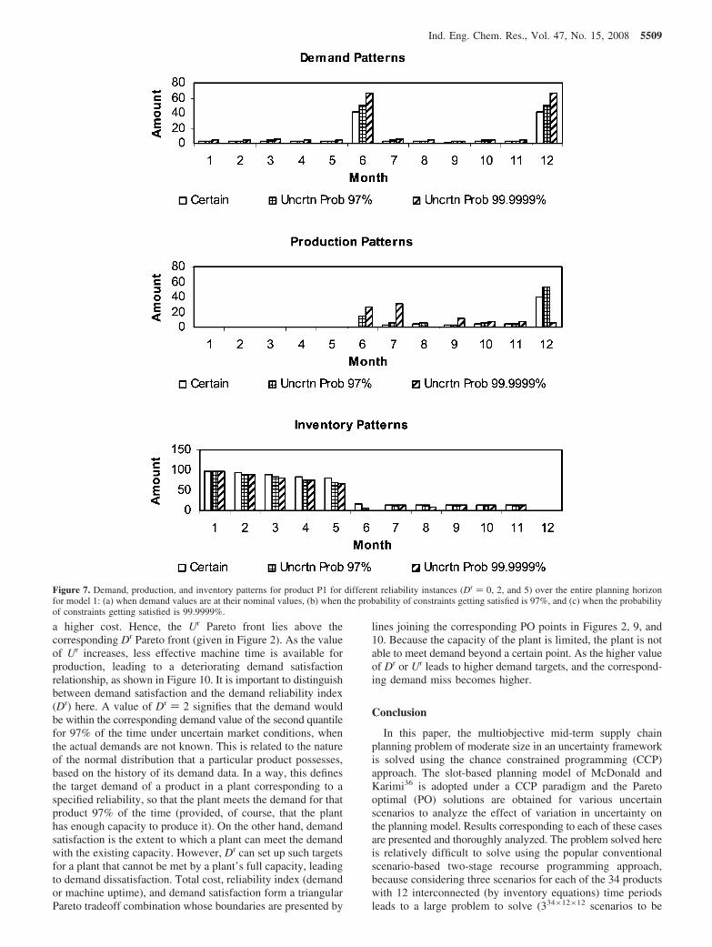
) 0), while the other two cases are when demands must besatisfied with 97% (Dr ) 2) and 99.9999% (Dr ) 5) probabilityat 10% demand variation (corresponding to PO points A and Cin Figure 2). As this probability value increases, greater demandfor the products appears and products are made in greateramounts to combat the uncertainty associated with demand, ascan be observed in Figure 6. Similar predictions for model 1can be observed in the results presented in Figure 7.

Assessing Uncertainty: Variation in Machine UptimeReliability Index. Machine utilization for machine 1 atproduction site 1 improves from an average value of 77%for the nominal case to an average value of 95% for the 10%standard deviation case and 100% for the 15% standarddeviation case for Dr ) 2 (model 2). During the study,machine 2 was never observed as a resource limiting oneand, therefore, had average uptime values of 20%, 24%, and24% for the nominal, 10%, and 15% standard deviation cases,respectively, for the same value of Dr (Figure 8). The machineat site S2 is not capacity-limiting; therefore, we analyzedthe machine at site S1 further. When the machine was fullyutilized (e.g., Dr ) 2 and 15% demand standard deviation),we introduced an upstream uncertainty in the machineavailability. To handle the additional scenario of machineuncertainty, eqs 30, 32, and 33 are included in model 1 in

Figure 3. Break-up cost components of the total cost for the corresponding Pareto optimal (PO) solutions in a cost-versus-demand reliability index (Dr)curve.

Figure 4. Demand, production, and inventory patterns for product P1 undervarious demand uncertainties over the entire planning horizon for model 2:(a) when demand values are at their nominal values, (b) when the standarddeviation of demands are 10% of the nominal values, and (c) when thestandard deviation of demands are 15% of the nominal values.

Ind. Eng. Chem. Res., Vol. 47, No. 15, 2008 5507

place of eqs 8, 19, and 20, respectively, and eqs 31–34 areincluded in model 2 in place of eqs 8, 9, 19, 20, and 21,respectively.

In the aforementioned analysis, we have observed that thedemand sought from the market is met with a reasonable degreeof demand satisfaction. However, from a practical viewpoint,there may be various instances of uncertain situations that canlead to uncertainty in the upstream processes for which demandis difficult to meet, to the fullest extent. Machine downtime dueto power failures or some maintenance problem, for example,can be examples of such upstream uncertainties. If machine

uptime reliability index (MURI), Ur, is defined in the same waythat the demand reliability index (Dr) was defined, a similarPareto tradeoff (see Figure 9) can be observed between the totalcost and MURI for a fixed value of Dr. The Pareto curve forthe total cost versus machine uptime reliability has beengenerated for different instances of Ur values, keeping Dr ) 2and a demand and machine uptime standard deviation of 15%of the corresponding nominal values. As we go for more-reliableuptime models for a fixed value of Dr, we have a tendency toincur a higher cost. In this case, the reliability considers bothdemand and machine uptime uncertainty and, therefore, incurs

Figure 5. Demand, production, and inventory patterns for product P1 undervarious demand uncertainties over the entire planning horizon for model 1:(a) when demand values are at their nominal values, (b) when the standarddeviation of demands are 10% of the nominal values, and (c) when thestandard deviation of demands 15% of the nominal values.

Table 1. Production Figures for All Product Families for Production Site S1 and Products for Production Site S2 for Model 2 for the EntirePlanning Horizon at Dr ) 2 and the Standard Deviation of the Products is 10% of Their Nominal Demands

t1 t2 t3 t4 t5 T6 t7 t8 t9 T10 t11 t12

F1 117.7 84.5F2 17.5F3 7.6 148.3 22.7 21.8 114.4F4 50.1 49.3 72.2F5 88.5 63.4F6 32.1 27.3F7 81.1F8 151.1 30.0 20.4 46.2 65.7F9 170.2 12.6 76.6 58.8F10 87.9 145.6 127.5 88.9 22.8 26.0 224.0 48.2F11 39.8 32.9P24 9.0 1.8 2.0 1.7 1.7 25.2 2.2 1.8 1.2 1.9 1.7 17.9P25 0.0 0.1 0.0 0.0 0.0 0.4 0.0 0.0 0.1 0.0 0.0 0.4P26 1.8 0.4 3.6 0.2 0.4 0.2 0.2 0.2 2.6P27 8.7 1.8 1.9 1.7 1.7 25.2 1.7 1.8 1.2 1.7 1.7 18.2P28 9.3 1.9 1.8 1.8 1.7 27.0 1.8 1.8 1.9 1.8 1.8 19.5P29 2.6 0.4 0.2 7.2 0.4 0.5 0.2 0.5 0.4 7.5P30 0.7 0.4P31 2.6 2.0 0.4 7.2 0.6 0.6 0.6 0.6 0.5 4.7P32 16.5 3.6 3.0 2.9 3.7 45.0 3.0 3.1 3.7 3.5 2.9 38.7P33 31.0 6.5 6.2 6.0 8.0 84.4 5.8 5.4 5.0 5.3 5.3 51.6P34 3.6 0.5 0.5 7.2 0.5 0.5 0.5 0.5 0.5 5.2

Figure 6. Demand, production, and inventory patterns for product P1 fordifferent reliability instances (Dr ) 0, 2, and 5) over the entire planninghorizon for model 2: (a) when demand values are at their nominal values,(b) when the probability of constraints getting satisfied is 97%, and (c)when the probability of constraints getting satisfied is 99.9999%.

5508 Ind. Eng. Chem. Res., Vol. 47, No. 15, 2008

a higher cost. Hence, the Ur Pareto front lies above thecorresponding Dr Pareto front (given in Figure 2). As the valueof Ur increases, less effective machine time is available forproduction, leading to a deteriorating demand satisfactionrelationship, as shown in Figure 10. It is important to distinguishbetween demand satisfaction and the demand reliability index(Dr) here. A value of Dr ) 2 signifies that the demand wouldbe within the corresponding demand value of the second quantilefor 97% of the time under uncertain market conditions, whenthe actual demands are not known. This is related to the natureof the normal distribution that a particular product possesses,based on the history of its demand data. In a way, this definesthe target demand of a product in a plant corresponding to aspecified reliability, so that the plant meets the demand for thatproduct 97% of the time (provided, of course, that the planthas enough capacity to produce it). On the other hand, demandsatisfaction is the extent to which a plant can meet the demandwith the existing capacity. However, Dr can set up such targetsfor a plant that cannot be met by a plant’s full capacity, leadingto demand dissatisfaction. Total cost, reliability index (demandor machine uptime), and demand satisfaction form a triangularPareto tradeoff combination whose boundaries are presented by

lines joining the corresponding PO points in Figures 2, 9, and10. Because the capacity of the plant is limited, the plant is notable to meet demand beyond a certain point. As the higher valueof Dr or Ur leads to higher demand targets, and the correspond-ing demand miss becomes higher.

Conclusion

In this paper, the multiobjective mid-term supply chainplanning problem of moderate size in an uncertainty frameworkis solved using the chance constrained programming (CCP)approach. The slot-based planning model of McDonald andKarimi36 is adopted under a CCP paradigm and the Paretooptimal (PO) solutions are obtained for various uncertainscenarios to analyze the effect of variation in uncertainty onthe planning model. Results corresponding to each of these casesare presented and thoroughly analyzed. The problem solved hereis relatively difficult to solve using the popular conventionalscenario-based two-stage recourse programming approach,because considering three scenarios for each of the 34 productswith 12 interconnected (by inventory equations) time periodsleads to a large problem to solve (334×12×12 scenarios to be

Figure 7. Demand, production, and inventory patterns for product P1 for different reliability instances (Dr ) 0, 2, and 5) over the entire planning horizonfor model 1: (a) when demand values are at their nominal values, (b) when the probability of constraints getting satisfied is 97%, and (c) when the probabilityof constraints getting satisfied is 99.9999%.

Ind. Eng. Chem. Res., Vol. 47, No. 15, 2008 5509

considered). In our approach, the problem formulation is quitegeneric and easy to model and the time involved in solving theproblem is quite small. Because of these strong points, the CCPholds great potential in handling problems under uncertainty.

Nomenclature

Pi,j,s,t ) production amount of i ∈ I\IRM on processor j at facility sin time period t

RLi,j,s,t ) corresponding run length of product i ∈ I\IRM on processorj at facility s in time period t

Ci,s,t ) consumption of raw material or intermediate i ∈ I\IFP at afacility s in time period t

Ii,s,t ) inventory level for i ∈ I\IRM at the end of time period t atlocation s

Si,s,c,t ) supply of finished product i ∈ IFP from facility s to customerc in time period t

σi,s,s′,t ) flow of intermediate product i ∈ IIP from facility s to s′ intime period t

Ii,c,t- ) amount of shortage of finished product i ∈ IFP for customer

c in time period tIi,s,t∆ ) deviation below safety stock target for product i ∈ I at location

s in time period thist ) inventory cost for holding a unit of product i in inventory at

facility s for the duration of the time period tµic ) revenue per unit of product i ∈ IFP sold to customer cpis ) price of raw material i ∈ IRM at facility s�is ) penalty for dipping below safety target of product i at a site

sνijs ) variable cost to produce a unit of product i ∈ I\IRM on

processor j at site stss′/tsc ) transportation cost to move a unit of product from site s to

site s′ or customer cRijst ) effective rate for product i on processor j at facility s in

time period t (it includes adjustment to the rate relating toefficiency, utility, and/or yield as defined for a particularmanufacturing environment)

�i′is ) yield-adjusted amount of raw or intermediate i ∈ I\IFP thatmust be consumed to produce a unit of i′ ∈ I\IRM at facility s

Hjst ) amount of time available for production on processor j atfacility s during time period t

dict ) demand for finished product i for customer c due at end oftime period t

Ii,s,tL ) safety stock target for product i at facility s in time period

tIi,s0 ) inventory of product i held in facility s at start of planning

horizon

Literature Cited

(1) Shapiro, J. F. Modeling the Supply Chain; Brooks/Cole-ThomsonLearning: Pacific Grove, CA, 2001.

(2) Liu, M. L.; Sahinidis, N. V. Optimization in Process Planning underUncertainty. Ind. Eng. Chem. Res. 1996, 35, 4154.

(3) Liu, M. L.; Sahinidis, N. V. Robust Process Planning underUncertainty. Ind. Eng. Chem. Res. 1998, 37, 1883.

(4) Petkov, S. B.; Maranas, C. D. Design of Single-Product CampaignBatch Plants under Demand Uncertainty. AIChE J. 1998, 44, 896.

(5) Dantzig, G. B. Linear Programming Under Uncertainty. Man. Sci.1955, 1, 197.

(6) Ierapetritou, M. G.; Pistikopoulos, E. N.; Floudas, C. A. OperationalPlanning under Uncertainty. Comput. Chem. Eng. 1994, S18, S553.

(7) Ierapetritou, M. G.; Pistikopoulos, E. N. Simultaneous Incorporationof Flexibility and Economic Risk in Operational Planning Under Uncer-tainty. Comput. Chem. Eng. 1994a, 18, 163.

(8) Ierapetritou, M. G.; Pistikopoulos, E. N. Novel OptimizationApproach of Stochastic Planning Models. Ind. Eng. Chem. Res. 1994, 33,1930.

(9) Pistikopoulos, E. N. Uncertainty in Process Design and Operations.Comput. Chem. Eng. 1995, S19, S553.

(10) Pistikopoulos, E. N.; Ierapetritou, M. G. Novel Approach forOptimal Process Design under Uncertainty. Comput. Chem. Eng. 1995, 19,1089.

(11) Clay, R. L.; Grossmann, I. E. Optimization of Stochastic PlanningModels. Trans. Inst. Chem. Eng. 1994, 72, 415.

Figure 8. Machine utilization patterns for machine at site S1 and S2 fornominal demand and when the standard deviation of demand is 10% and15% of nominal demands for Dr ) 2 over the entire planning horizon formodel 2.

Figure 9. Total cost versus the machine uptime reliability index (MURI,Ur) Pareto front for different MURI values for model 2 (the standarddeviation values of uncertain demand are kept fixed at 15%, but the samefor machine uptime are kept at 10% and 15% of their nominal values).

Figure 10. Relationship of total cost versus demand satisfaction for differentMURI values for model 2, corresponding to the Pareto optimal (PO) pointspresented in Figure 9.

5510 Ind. Eng. Chem. Res., Vol. 47, No. 15, 2008

(12) Bellman, R.; Zadeh, L. A. Decision-making in a Fuzzy Environ-ment. Man. Sci. 1970, 17, 141.

(13) Zimmermann, H. J. Fuzzy Programming and Linear Programmingwith Several Objective Functions. Fuzzy Sets Syst. 1978, 1, 45.

(14) Zimmermann, H. J. Fuzzy Set Theory and Its Application; KluwerAcademic Publishers: Boston, 1991.

(15) Tanaka, H.; Okuda, T.; Asai, K. On Fuzzy Mathematical Program-ming. J. Cybernet. 1974, 3, 37.

(16) Delgado, M.; Herrera, F.; Verdegay, J. L.; Vila, M. A. Postopti-mality Analysis on the Membership Function of a Fuzzy Linear Program-ming Problem. Fuzzy Sets Syst. 1993, 53, 289.

(17) Tanaka, H.; Asai, K. Fuzzy Linear Programming Problems withFuzzy Numbers. Fuzzy Sets Syst. 1984, 13, 1.

(18) Tong, S. Interval Number and Fuzzy Number Linear Programming.Fuzzy Sets Syst. 1994, 66, 301.

(19) Prekopa, A. Stochastic Programming; Kluwer Academic Publishers:Dordrecht, The Netherlands, 1995.

(20) Birge, J. R.; Louveaux, F. Introduction to Stochastic Programming;Springer-Verlag: New York, 1994.

(21) Maranas, C. D. Optimal Molecular Design under Property PredictionUncertainty. AIChE J. 1997, 43, 1250.

(22) Kall, P.; Wallace, S. W. Stochastic Programming; Wiley: NewYork, 1994.

(23) Lakhdar, K.; Farid, S. S.; Titchener-Hooker, N. J.; Papageorgiou,L. G. Medium Term Planning of Biopharmaceutical Manufacture withUncertain Fermentation Titers. Biotechnol. Prog. 2006, 22, 1630.

(24) Charnes, A.; Cooper, W. W. Chance Constrained Programming.Man. Sci. 1958, 6, 73.

(25) Sahinidis, N. V. Optimization under Uncertainty: State-of-the-Artand Opportunities. Comput. Chem. Eng. 2004, 28, 971.

(26) Subrahmanyam, S.; Pekny, J. F.; Reklaitis, G. V. Design of BatchChemical Plants under Market Uncertainty. Ind. Eng. Chem. Res. 1994,33, 2688.

(27) Shah, N.; Pantelides, C. C. Design of Multipurpose Batch Plantswith Uncertain Production Requirements. Ind. Eng. Chem. Res. 1992, 31,1325.

(28) Liu, M. L.; Sahinidis, N. V. Long Range Planning in the ProcessIndustries: A Projection Approach. Comput. Oper. Res. 1996, 23, 237.

(29) Wellons, H. S.; Reklaitis, G. V. The Design of Multiproduct BatchPlants under Uncertainty with Staged Expansion. Comput. Chem. Eng. 1989,13, 115.

(30) Ierapetritou, M. G.; Pistikopoulos, E. N. Batch Plant Design andOperations under Uncertainty. Ind. Eng. Chem. Res. 1996, 35, 772.

(31) Dantzig, G. B.; Wolfe, P. The Decomposition Principle for LinearProgram. Oper. Res. 1960, 8, 101.

(32) Benders, J. F. Partitioning Procedures for Solving Mixed VariablesProgramming Problems. Num. Math. 1962, 4, 238.

(33) Diwekar, U. M.; Kalagnanam, J. R. Efficient Sampling Techniquefor Optimization under Uncertainty. AIChE J. 1997, 43, 440.

(34) Gupta, A.; Maranas, C. D. A Two-Stage Modeling and SolutionFramework for Multisite Midterm Planning under Demand Uncertainty. Ind.Eng. Chem. Res. 2000, 39, 3799.

(35) Gupta, A.; Maranas, C. D. Managing Demand Uncertainty in SupplyChain Planning. Comput. Chem. Eng. 2003, 27, 1219.

(36) McDonald, C. M.; Karimi, I. A. Planning and Scheduling of ParallelSemicontinuous Processes. 1. Production Planning. Ind. Eng. Chem. Res.1997, 36, 2691.

(37) Brooke, A.; Kendrick, D.; Meeraus, A. GAMS;A User’s Guide;GAMS Development Corporation: Washington, DC, 1998.

(38) Haimes, Y. Y.; Lasdon, L. S.; Wismer, D. A. On a BicriterionFormulation of the Problems of the Integrated System Identification andSystem Optimization. IEEE Trans. Syst., Man. Cybernet. 1971, 1, 296.

(39) Chankong, V.; Haimes, Y. Y. MultiobjectiVe Decision MakingTheory and Methodology; North-Holland: New York, 1983.

(40) Miettinen, K. Nonlinear MultiobjectiVe Optimization; KluwerAcademic Publishers: Boston, 1999.

(41) Charnes, A.; Cooper, W.; Ferguson, R. Optimal Estimation ofExecutive Compensation by Linear Programming. Man. Sci. 1955, 1, 138.

(42) Ignizio, J. P. Goal Programming and Extensions; Lexington Books:Lexington, MA, 1976.

(43) Ignizio, J. P. A Review of Goal Programming: A Tool forMultiobjective Analysis. J. Oper. Res. Soc. 1978, 29, 1109.

(44) Lee, S. M. Goal Programming for Decision Analysis; AuerbachPublishers: Philadelphia, 1972.

(45) Romero, C. Handbook of Critical Issues in Goal Programming;Pergamon Press: Oxford, U.K., 1991.

(46) Steuer, R. E. Multiple Criteria Optimization: Theory, Computationand Applications; Wiley: New York, 1986.

ReceiVed for reView July 30, 2007ReVised manuscript receiVed April 10, 2008

Accepted April 23, 2008

IE0710364

Ind. Eng. Chem. Res., Vol. 47, No. 15, 2008 5511