Master Thesis Electrical Engineering Thesis no: MEE-2008:25 July 2008 Analysis of MIG Welding with Aim on Quality Irina Gertsovich Niklas Svanberg Department of Signal Processing Areva Uddcomb Engineering Blekinge Institute of Technology Port Chapman Box 520 371 21 Karlskrona SE - 372 25 Ronneby Sweden
Department of Signal Processing Areva Uddcomb EngineeringBlekinge Institute of Technology Port ChapmanBox 520 371 21 KarlskronaSE - 372 25 RonnebySweden
This thesis is submitted to the School of Engineering at Blekinge Institute of Technologyin partial fulfillment of the requirements for the degree of Master of Science in ElectricalEngineering. The thesis is equivalent to 2 x 20 weeks of full time studies.
External advisor :Nils BjerstenUddcomb Engineering AB
University advisor and examiner :Mikael NilssonDepartment of Signal Processing, BTH
University advisors :Josef Ström BartunekDepartment of Signal Processing, BTH
Department of Signal Processing Internet : www.bth.se/tekBlekinge Institute of Technology Phone : +46 457 38 50 00Box 520 Fax : +46 457 271 25SE - 372 25 RonnebySweden
ABSTRACT
Since 1987 Uddcomb Engineering has repaired pulps bytheir own developed overlay welding method even calledUddcomb method. Currently each welding machine is op-erated by two persons. To increase Uddcomb Engineeringcompetitiveness the reduced number of operators is de-sired. An installation of a monitoring system which canaid humans in the welding quality control also helps to im-prove company’s position. A future goal would be to makethis monitoring system automatic without a human opera-tor in the loop.
In this thesis, arc voltage, weld current and audio sig-nals were collected and analyzed with aim on finding algo-rithms to monitor the quality of the welding process. Theuse of statistics tools is the basis for detecting variations inthe voltage and current data, associated with welding pro-cess. It has been shown that voltage signal can be usedas a part of the welding quality control. The audio sig-nal from welding at low frequencies varies with the speedof the process. The signal can also be incorporated in themonitoring of the process.
The use of filters, growing sums and statistics are keyelements in the algorithms presented in this report.
Keywords: MIG welding, Arc Voltage, Weld Cur-rent, Audio, Signal Processing.
2.1 Overview of MIG/MAG welding equipment. 1) power source, 2) welding gun, 3) electrodebobbin, 4) wire feeder, 5) controller, 6) water supply, 7) gas supply, and 8) workpiece. . . 4
2.2 Characteristics of the power source; a) dropping b) straight c) lightly dropping. . . . . . 42.3 The welding gun. 1) the gas hose, 2) the contact tube, and 3) the electrode wire. . . . . 52.4 The end tip of the welding gun [1, p40]. 1) electrode wire, 2) contact piece, 3) gas(es),
4) drops of electrode wire, 5) area of gases, and 6) the arc area. . . . . . . . . . . . . . 52.5 Schematic of the voltage drop in the arc [1]. Le denotes the electrode stick-out from the
contact tube, La denotes the arc length, Ua, Uco and Uc denote the anode, column andcathode voltage drop respectively. . . . . . . . . . . . . . . . . . . . . . . . . . . . . . 7
4.2 Pulses generated by the welding power source. . . . . . . . . . . . . . . . . . . . . . . 124.3 Schematic of sound measurement. . . . . . . . . . . . . . . . . . . . . . . . . . . . . 134.4 Schematic of current measurement. . . . . . . . . . . . . . . . . . . . . . . . . . . . 134.5 Schematic of the voltage splitter. . . . . . . . . . . . . . . . . . . . . . . . . . . . . . 144.6 Schematic of video monitoring and recording. . . . . . . . . . . . . . . . . . . . . . . 144.7 Picture of the fingercamera. The units on the ruler are centimeters. . . . . . . . . . . . 154.8 (a) Overview of the workpiece (b) Description of which surfaces the workpiece are divided
into and also how long they are. . . . . . . . . . . . . . . . . . . . . . . . . . . . . . 164.9 Graphical User Interface (GUI) used during the data collection. . . . . . . . . . . . . . 174.10 Visual welding results from measurements 4-9. The upper numbers indicate with electrode
wire type used and the lower numbers are the wire speed [m/min]. . . . . . . . . . . . . 194.11 Visual welding results from measurements 1-3 and 10-12. The upper numbers indicate
with electrode wire type used and the lower numbers are the wire speed [m/min]. . . . . . 194.12 Visual welding results from measurements 13-14. Measurement setup: electrode wire 29.9
5.1 M1 in time domain, where (b) is only a part of the total signal in (a). . . . . . . . . . . 215.2 M11 in time domain, where (b) is only a part of the total signal in (a). . . . . . . . . . 225.3 M1 statistics measures of different block sizes; (a) Mean (b) Variance; Solid line is surface
1 and dashed line is surface 2. . . . . . . . . . . . . . . . . . . . . . . . . . . . . . . 235.4 M5 statistics measures of different block sizes; (a) Mean (b) Variance; Solid line is surface
3, dashed line is surface 4 and dashdotted line is surface 5. . . . . . . . . . . . . . . . 235.5 Block statistics test for stationarity with 4410 samples/block on surface 1(60 seconds) in
5.7 M1 statistics measures of different block sizes; (a) Mean (b) Variance; Solid line is surface1 and dashed line is surface 2. . . . . . . . . . . . . . . . . . . . . . . . . . . . . . . 25
5.8 M5 statistics measures of different block sizes; (a) Mean (b) Variance; Solid line is surface3, dashed line is surface 4 and dashdotted line is surface 5. . . . . . . . . . . . . . . . 25
5.9 Block statistics test for stationarity with 4410 samples/block on surface 1(60 seconds) inM1; (a) Mean (b) Variance. . . . . . . . . . . . . . . . . . . . . . . . . . . . . . . . 26
5.10 Histogram of (a) M1 (b) M11. . . . . . . . . . . . . . . . . . . . . . . . . . . . . . . 265.11 M1; (a) shows the current data with the rapidly changing characteristic when switching
row in welding process; (b) shows the voltage and it’s transients. . . . . . . . . . . . . . 275.12 M1; (a) shows the current data with the rapidly changing characteristic when switching
row in welding process; (b) shows the voltage and it’s transients. . . . . . . . . . . . . . 285.13 M1; (a) shows the current data with the rapidly changing characteristic when switching
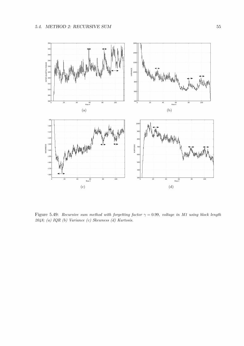
5.41 Recursive sum method for voltage in M1 using block length 2048; (a) Variance (b) Skewness 505.42 Recursive sum method for voltage in M11 using block length 2048; (a) Variance (b) Skewness 515.43 Recursive sum method for voltage in M5 using block length 2048; (a) Variance (b) Skewness 515.44 Recursive sum method for voltage in M8 using block length 2048; (a) Variance (b) Skewness 525.45 Recursive sum method for current in M1 using block length 2048; (a) Variance (b) Skewness 525.46 Recursive sum method for current in M11 using block length 2048; (a) Variance (b) Skewness 535.47 Recursive sum method for current in M5 using block length 2048; (a) Variance (b) Skewness 535.48 Recursive sum method for current in M8 using block length 2048; (a) Variance (b) Skewness 545.49 Recursive sum method with forgetting factor γ = 0.99, voltage in M1 using block length
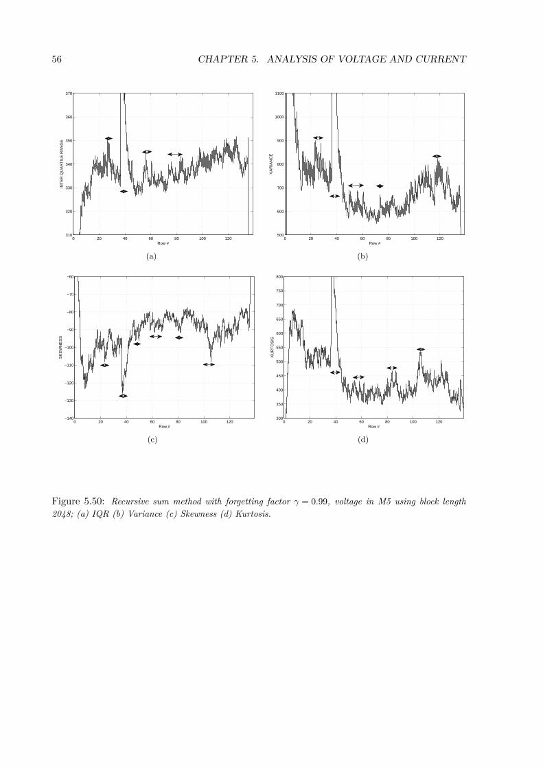
2048; (a) IQR (b) Variance (c) Skewness (d) Kurtosis. . . . . . . . . . . . . . . . . . 555.50 Recursive sum method with forgetting factor γ = 0.99, voltage in M5 using block length
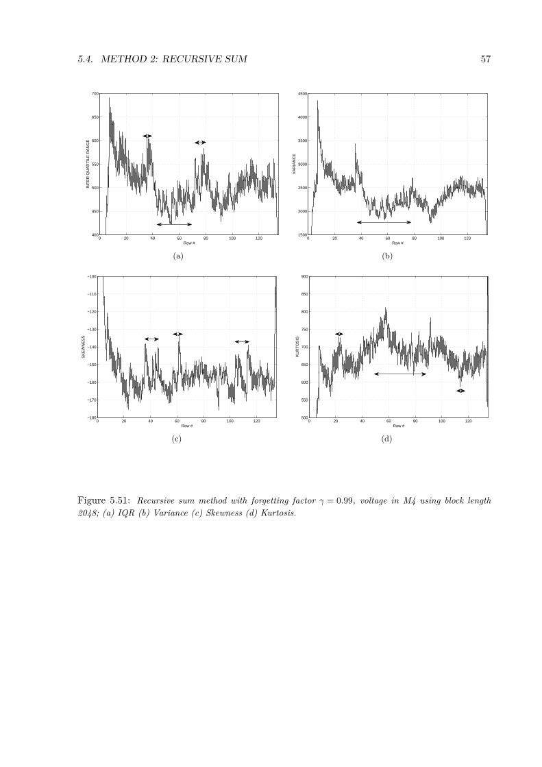
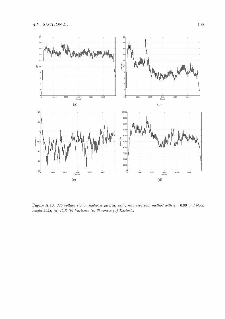
2048; (a) IQR (b) Variance (c) Skewness (d) Kurtosis. . . . . . . . . . . . . . . . . . 565.51 Recursive sum method with forgetting factor γ = 0.99, voltage in M4 using block length
2048; (a) IQR (b) Variance (c) Skewness (d) Kurtosis. . . . . . . . . . . . . . . . . . 575.52 M1 voltage signal, highpass filtered, using recursive sum method with γ = 0.99 and block
length 2048; (a) IQR (b) Variance (c) Skewness (d) Kurtosis. . . . . . . . . . . . . . . 595.53 M2 voltage signal, highpass filtered, using recursive sum method with γ = 0.99 and block
length 2048; (a) IQR (b) Variance (c) Skewness (d) Kurtosis. . . . . . . . . . . . . . . 605.54 M3 voltage signal, highpass filtered, using recursive sum method with γ = 0.99 and block
length 2048; (a) IQR (b) Variance (c) Skewness (d) Kurtosis. . . . . . . . . . . . . . . 615.55 M10 voltage signal, highpass filtered, using recursive sum method with γ = 0.99 and block
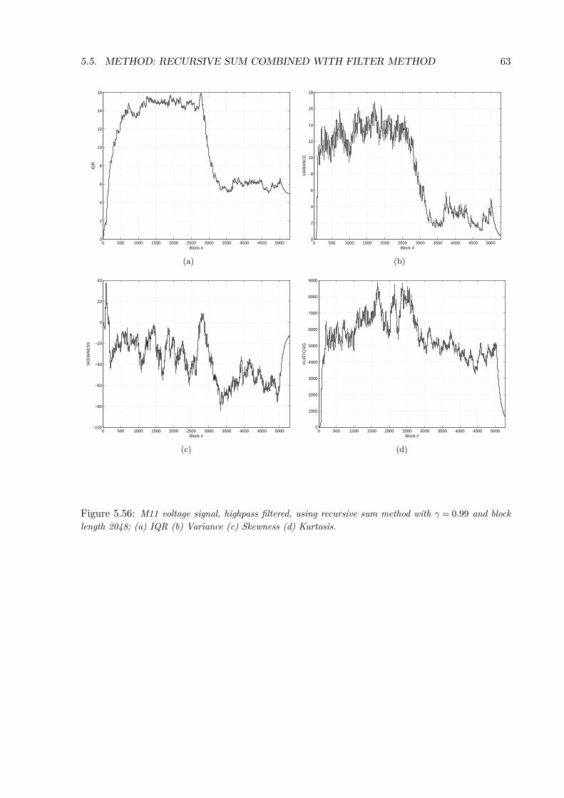
length 2048; (a) IQR (b) Variance (c) Skewness (d) Kurtosis. . . . . . . . . . . . . . . 625.56 M11 voltage signal, highpass filtered, using recursive sum method with γ = 0.99 and block
length 2048; (a) IQR (b) Variance (c) Skewness (d) Kurtosis. . . . . . . . . . . . . . . 635.57 M12 voltage signal, highpass filtered, using recursive sum method with γ = 0.99 and block
length 2048; (a) IQR (b) Variance (c) Skewness (d) Kurtosis. . . . . . . . . . . . . . . 645.58 M1 voltage signal, highpass filtered, using recursive sum method with γ = 0.99 and block
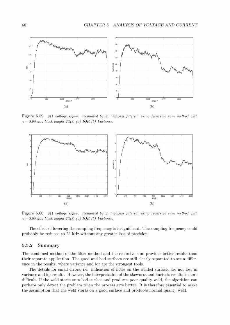
length 2048; (a) IQR (b) Variance. . . . . . . . . . . . . . . . . . . . . . . . . . . . . 655.59 M1 voltage signal, decimated by 2, highpass filtered, using recursive sum method with
γ = 0.99 and block length 2048; (a) IQR (b) Variance. . . . . . . . . . . . . . . . . . . 665.60 M1 voltage signal, decimated by 3, highpass filtered, using recursive sum method with
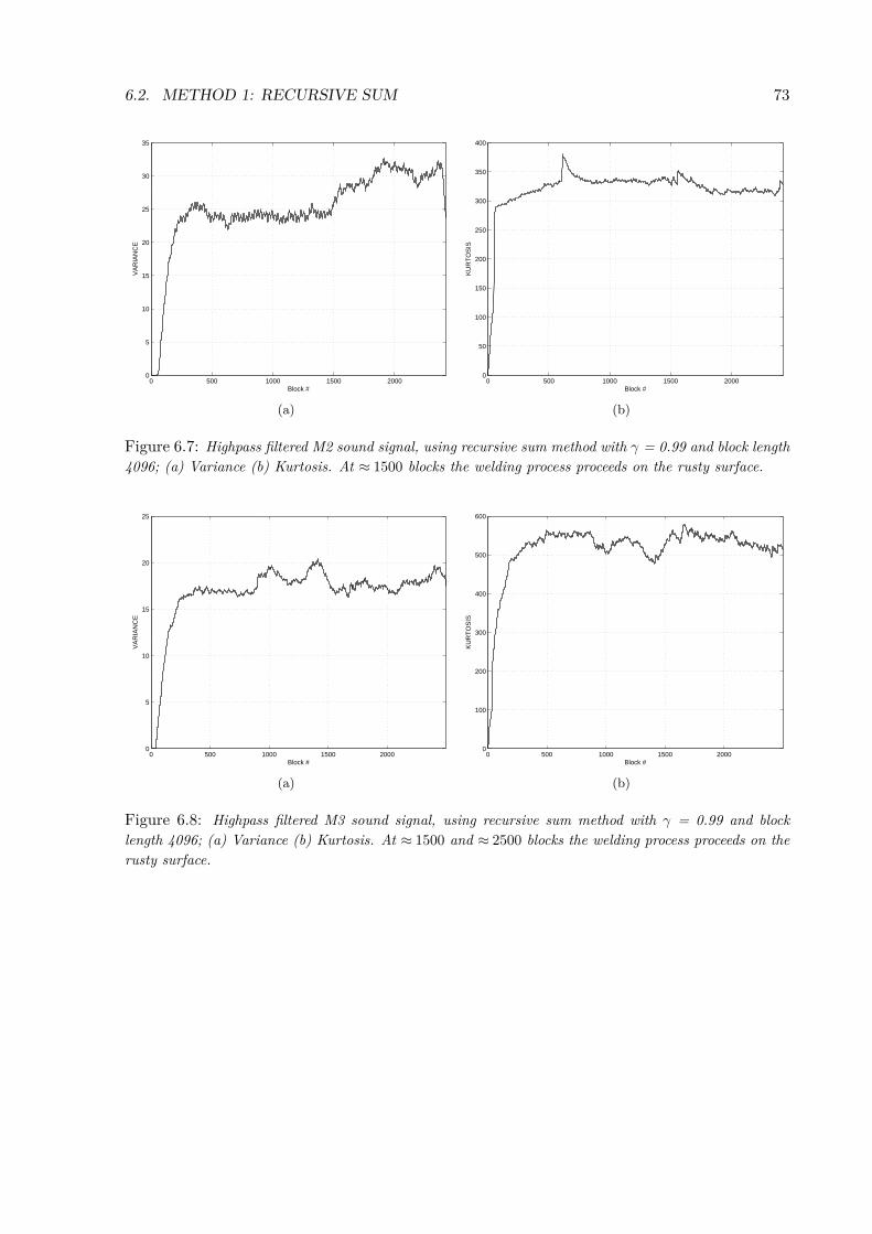
6.7 Highpass filtered M2 sound signal, using recursive sum method with γ = 0.99 and blocklength 4096; (a) Variance (b) Kurtosis. At ≈ 1500 blocks the welding process proceeds onthe rusty surface. . . . . . . . . . . . . . . . . . . . . . . . . . . . . . . . . . . . . . 73
10 LIST OF FIGURES
6.8 Highpass filtered M3 sound signal, using recursive sum method with γ = 0.99 and blocklength 4096; (a) Variance (b) Kurtosis. At ≈ 1500 and ≈ 2500 blocks the welding processproceeds on the rusty surface. . . . . . . . . . . . . . . . . . . . . . . . . . . . . . . . 73
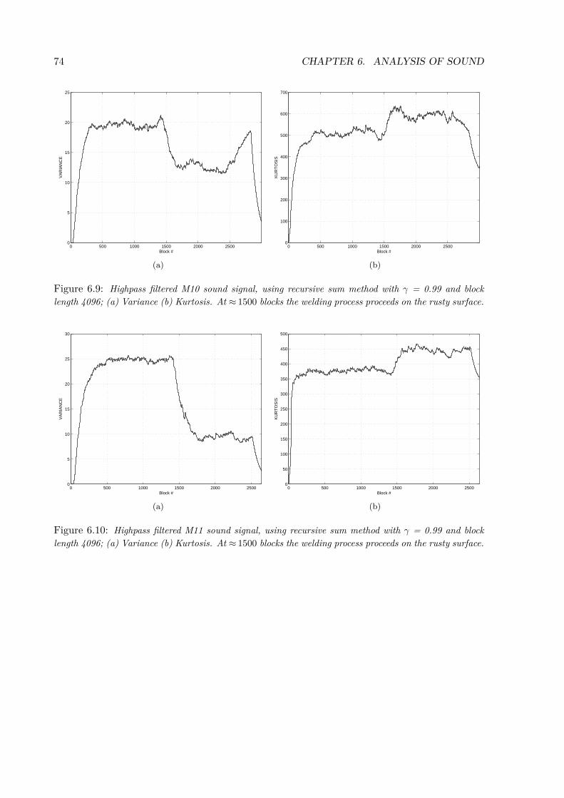
6.9 Highpass filtered M10 sound signal, using recursive sum method with γ = 0.99 and blocklength 4096; (a) Variance (b) Kurtosis. At ≈ 1500 blocks the welding process proceeds onthe rusty surface. . . . . . . . . . . . . . . . . . . . . . . . . . . . . . . . . . . . . . 74
6.10 Highpass filtered M11 sound signal, using recursive sum method with γ = 0.99 and blocklength 4096; (a) Variance (b) Kurtosis. At ≈ 1500 blocks the welding process proceeds onthe rusty surface. . . . . . . . . . . . . . . . . . . . . . . . . . . . . . . . . . . . . . 74
6.11 Highpass filtered M12 sound signal, using recursive sum method with γ = 0.99 and blocklength 4096; (a) Variance (b) Kurtosis. At ≈ 1500 blocks the welding process proceeds onthe rusty surface. . . . . . . . . . . . . . . . . . . . . . . . . . . . . . . . . . . . . . 75
6.12 Highpass filtered M13 sound signal, using recursive sum method with γ = 0.99 and blocklength 4096; (a) Variance (b) Kurtosis. At ≈ 1500 blocks the welding process proceeds onthe rusty surface. . . . . . . . . . . . . . . . . . . . . . . . . . . . . . . . . . . . . . 75
6.13 Lowpass filter with pass band 1 Hz and transition band 90 Hz. . . . . . . . . . . . . . . 776.14 Spectrogram of the audio record for first surface in M12. Zoomed at frequency range 0 -
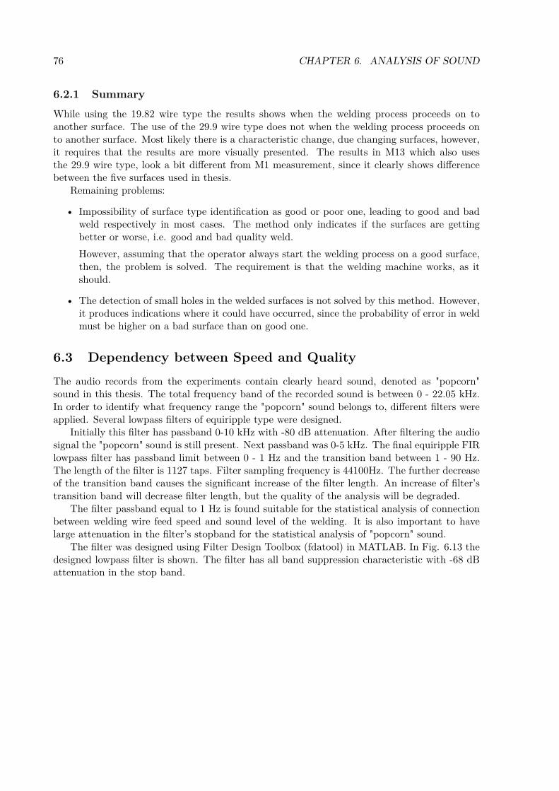
500 Hz. . . . . . . . . . . . . . . . . . . . . . . . . . . . . . . . . . . . . . . . . . . 776.15 Spectrogram of second surface in M2. The power of the signal is around -60 dB for the
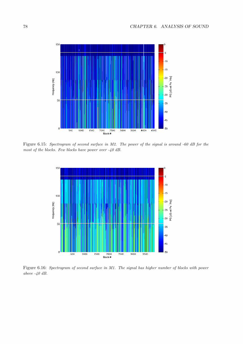
most of the blocks. Few blocks have power over -40 dB. . . . . . . . . . . . . . . . . . 786.16 Spectrogram of second surface in M1. The signal has higher number of blocks with power
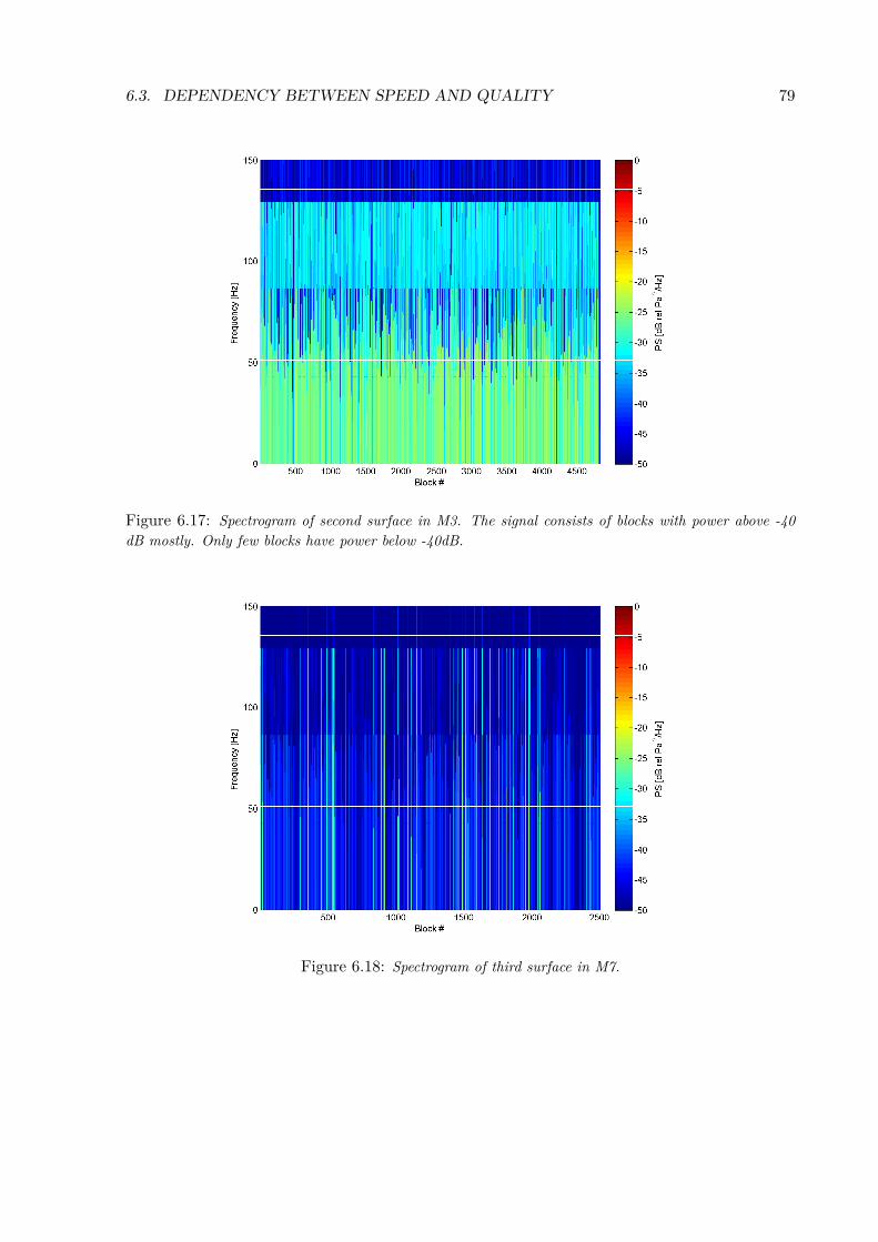
above -40 dB. . . . . . . . . . . . . . . . . . . . . . . . . . . . . . . . . . . . . . . . 786.17 Spectrogram of second surface in M3. The signal consists of blocks with power above -40
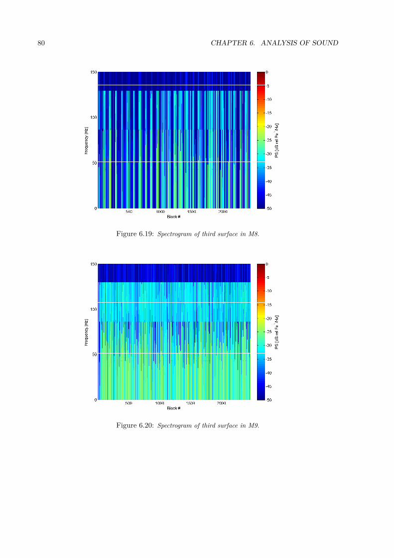
dB mostly. Only few blocks have power below -40dB. . . . . . . . . . . . . . . . . . . . 796.18 Spectrogram of third surface in M7. . . . . . . . . . . . . . . . . . . . . . . . . . . . 796.19 Spectrogram of third surface in M8. . . . . . . . . . . . . . . . . . . . . . . . . . . . 806.20 Spectrogram of third surface in M9. . . . . . . . . . . . . . . . . . . . . . . . . . . . 806.21 Statistical data example for M2, surface 2 only, calculated from signal power; (a) Mean
(b) Variance (c) Skewness (d) Kurtosis. . . . . . . . . . . . . . . . . . . . . . . . . . 826.22 Statistical data example for M2, surface 2 only, smoothed signal power; (a) Mean (b)
Variance (c) Skewness (d) Kurtosis. . . . . . . . . . . . . . . . . . . . . . . . . . . . 836.23 Mean of sound power for each speed group; (a) Original (b) Zoomed. . . . . . . . . . . 846.24 Mean value of averaged variance for each speed group; (a) Original (b) Zoomed. . . . . . 856.25 Power Spectral Density (PSD) using Welch periodogram method on M1. . . . . . . . . . 866.26 Power Spectral Density (PSD) using Welch periodogram method on M14. . . . . . . . . 87
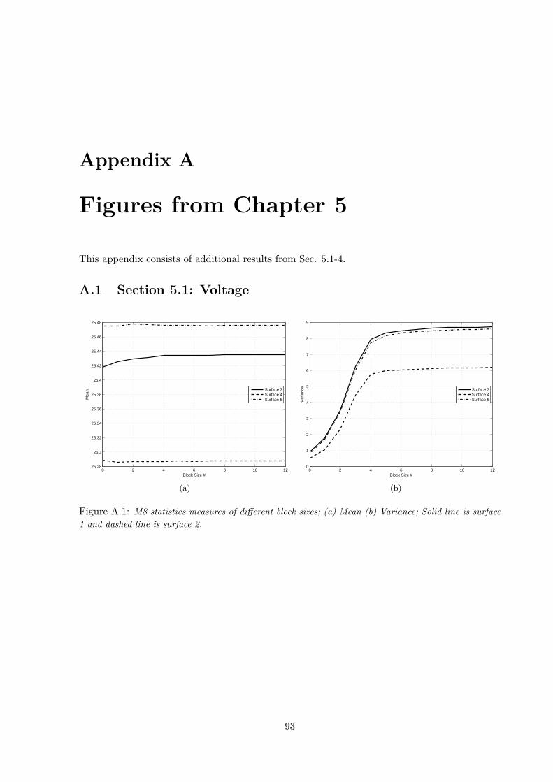
A.1 M8 statistics measures of different block sizes; (a) Mean (b) Variance; Solid line is surface1 and dashed line is surface 2. . . . . . . . . . . . . . . . . . . . . . . . . . . . . . . 93
A.2 M11 statistics measures of different block sizes; (a) Mean (b) Variance; Solid line issurface 3, dashed line is surface 4 and dashdotted line is surface 5. . . . . . . . . . . . 94
A.3 M8 statistics measures of different block sizes; (a) Mean (b) Variance; Solid line is surface1 and dashed line is surface 2. . . . . . . . . . . . . . . . . . . . . . . . . . . . . . . 94
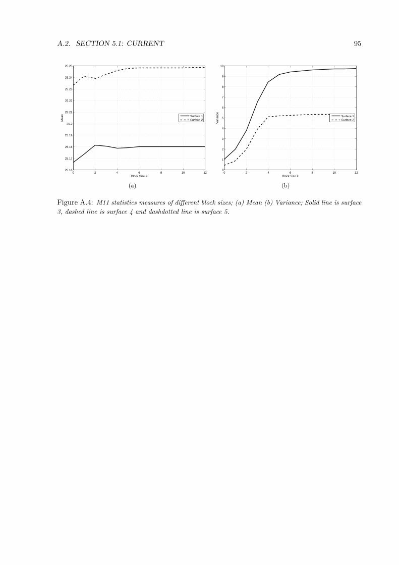
A.4 M11 statistics measures of different block sizes; (a) Mean (b) Variance; Solid line issurface 3, dashed line is surface 4 and dashdotted line is surface 5. . . . . . . . . . . . 95
4.1 The chemical composite in percent of wire 19.82. . . . . . . . . . . . . . . . . . . . . . 124.2 The chemical composite in percent of wire 29.9. . . . . . . . . . . . . . . . . . . . . . 124.3 Specifications of the used computers for collecting and storing sensor information. . . . 154.4 Specifications of used number of channels and sampling frequency when collection data
from current and voltage sensors (UA) and from two microphone sensors (UB). . . . . 154.5 Summary of the measurements setup. . . . . . . . . . . . . . . . . . . . . . . . . . . 18
5.1 Upper row is the true size and lower row is the number seen in Figs. 5.3-5.4 and 5.7-5.8. 22
This thesis has been preformed at Department of Signal Processing (ASB) at Blekinge Instituteof Technology (BTH/BIT) in cooperation with Uddcomb Engineering AB (UE). The thesis ison D-level and extends of 30 credit points.
1.1 BackgroundThe most pressure vessels in Swedish pulp industry was built during the 50th and 60th. Thesepulp vessels were constructed with black iron according to the methods, rules and regulationsof that time which fulfilled the corrosion analytical value of about 0.5 mm/year. As the timepassed, new demands arose within the pulp industry on faster and more environmental-friendlymethods. These new demands increased the yearly corrosion significant, which lead to the min-imum allowed thickness of pulp vessels was reached many years earlier than expected [2].
Uddcomb Engineering AB has since 1987 repaired pulp vessels by welding a new layer of rustlessiron on the vessels inside by primarily using semi-automated MIG welding machines.
Each machine is controlled by two operators, the first one controlling it and monitoring thewelding process, while the other one is monitoring the resulting quality of the weld. Normallya couple of these machines operate inside the pulp vessel at the same time, which with all itssound, lightning flashes, smoke, heat etc, creates together a general poor working environment.
1.2 PurposeCollect relevant information that is current, voltage, audio and video to perform the analysis ofthe welding process remotely. The collection of information should be preformed in cooperationwith a human expert in the area to create a transcribed database. Further, develop and evaluatealgorithms with the aim to imitate the human expert for welding quality control.
1
Chapter 2
Welding
2.1 Introduction
What is welding? The process where two or more metal materials are attached to each other.It is the basic of welding. There exist different variants of attachment methods.
Welding has been used by mankind for centuries. One method that has been used is namedforge welding. The metal is heated to its melting point and then is stricken by a hammer to betransformed to the desired shape.
In the end of 18th century some new methods of welding were discovered, such as resistanceand arc welding. The resistance welding method is based on Michael Faraday discovery. Thediscovery was if two steel objects are pressed together under the current flow influence, thenthe resistance between these objects creates a heat. The heat intensity is high enough to meltthe objects at their point of contact on the current path. This is method very well used in thecar industry and white goods industry [3, p8]. Arc welding on the other hand is performed byconnecting the workpiece to one pole of the power source and a coalpiece to the other. An elec-tric arc pass between coalpiece (electrode piece) and the workpiece which created high enoughenergy to melt the two pieces together. The coal piece was later replaced by a metal piece,which is known as metal arc welding.
In the early mid 19th century, experiments were made to find better methods which were nottime consuming, due to change of electrode pieces. The solution is known as Metal Inert Gas(MIG) or half automatic welding. The method uses a machine that automatically pushes anelectrode wire forward to the electric arc and is protected from oxidation with help of an inertgas, such as argon (Ar). Since the inert gases are expensive to produce, another method calledMetal Active Gas (MAG) was invented, where a chemical gas, such as carbon dioxide (CO2)is used instead. In this thesis a mix of these two methods has been used, which is describedfurther in this chapter.
Welding methods are generally placed in one of two main groups denoted spot welding and au-togenous welding [3, p17]. In autogenous welding the workpiece is heated to it’s melting point,where it is melted together with extra material. In spot welding the two pieces are pressedtogether with or without any heating. The method used in this thesis belongs to autogenouswelding and is part of Gas Metal Arc (GMA) welding.
3
4 CHAPTER 2. WELDING
2.2 Equipment in MIG/MAG WeldingIn this section the different equipment parts of MIG/MAG welding will be explained. Specificdetails about the equipments used in this thesis will be presented further in chapter 4. Theequipment consists of power source, welding gun, electrode bobbin, rod feeder, and some extraequipment. See Fig. 2.1 for an overview of the welding equipment.
-+
1
2
3
4
5
6
7
8
Figure 2.1: Overview of MIG/MAG welding equipment. 1) power source, 2) welding gun, 3) electrodebobbin, 4) wire feeder, 5) controller, 6) water supply, 7) gas supply, and 8) workpiece.
The electrode wire on the bobbin is continuously fed forward by the wire feeder to the electric arcat a constant speed. Normally the feeding speed is between 2 and 20 m/min [3, p85]. The powersource, water and gas supply are fed trough the controller and thereafter are linked together ina hose, which leads to the welding gun.
2.2.1 Power SourceThe power source used in MIG/MAG welding is mostly direct current (DC) with it’s positivepole connected to the electronic rod while the negative pole connected to the workpiece. Thepower source characteristics are very important for welding stability, ignition of the arc andtransfer of melted electrode wire to the workpiece. Characteristics of a power source can eitherbe dropping, straight or lightly dropping, where the two latter one are used in MIG/MAG. Fig.2.2 shows the characteristics of a power source between current and voltage.
Vo
lta
ge
Current
a
b
c
Figure 2.2: Characteristics of the power source; a) dropping b) straight c) lightly dropping.
2.2. EQUIPMENT IN MIG/MAG WELDING 5
Straight and lightly dropping characteristics of the power source helps maintain control ofthe arc. The voltage determines the length of the arc while the current (Ampere) automaticallyregulates itself during welding. The necessary level for melting the electrode wire depends onthe speed welding wire feeding and the content of the wire.
2.2.2 Welding Gun
1 2 3
Figure 2.3: The welding gun. 1) the gas hose, 2) the contact tube, and 3) the electrode wire.
Fig. 2.3 shows a general overview of a welding gun. The welding gun is an important partof the welding process. Through it, the electrode wire, gases and the current flow to the electricarc. In case of high level current it is recommended to add cooling water to the flow. The gunmust be light, smooth in use and should be tolerant to the high temperature.
+
-
1
2
3
45 6
Figure 2.4: The end tip of the welding gun [1, p40]. 1) electrode wire, 2) contact piece, 3) gas(es), 4)drops of electrode wire, 5) area of gases, and 6) the arc area.
2.2.3 Bobbin and wire FeederThe wire feeder has an important purpose. It is supplying the welding gun with electrode wire.Depending on where the rod feeder is placed, compared to where the bobbin and welding gunis, the wire is either pushed or pulled. Pushed is most regularly used, and can handle wirelength up to 5m [1, p43]. Pulled on the other hand is not very common, but a use of bothpulled and pushed rod feeders can be found in the same system, one at the bobbin and one atthe welding gun. This is called push-pull feeding and can handle wire lengths up to 15m [1, p43].
6 CHAPTER 2. WELDING
The electrode wire is placed on a bobbin which is placed on a hub brake. This brake con-trols the friction and stops the rotation when needed. Friction on the electrode wire can causethat particles detach and jam either of the rod feeders. Therefore wire is mostly covered with athin layer of copper to make the feeding of electrode wire easier with less friction.
2.3 Extra material for weldingThe electrode wire is one extra material which normally has a diameter of 0.6 to 2.4 mm [3, p90].For massive electrodes diameters of 0.8, 1.0 or 1.2 mm are usually used, and for tube electrodesthe wire is a bit wider. Two important factors when selecting the wire are the composition andthe wire purity. The electrode should also be selected with respect to surface of the workpiece.
Gases are extra material too. The MIG consists mainly of either argon or helium, while MAGconsists of carbon dioxide. The purpose of the gas is to protect the welding electrode wire fromparticles in the air surrounding the workpiece. The gas also affects the welding properties, thepenetration depth into and the penetration width on the workpiece.
Argon is an inert gas which has good properties such as not reacting on other substances,low ionization potential and gives a stable gas flow due to its high density value.
Helium is another inert gas which has high ionization potential, the ability to lead heat whichincreases the heat of the arc and a slightly wider penetration. However it has a low density.Since Helium and Argon are inert gases, they are expensive to use.
Carbon dioxide is ordinary inexpensive gas which has good penetration and good ability towithstand any contaminations on the surfaces. However it dissolves in the arc and creates twosubstances, carbon monoxide and oxygen. The carbon monoxide is a lethal gas [4, p5]. Theoxygen might oxidize the electrode wire.
The workpiece can be unalloyed steel, low alloyed steel, high alloyed steel, aluminium alloyed,magnesium alloyed, titan alloyed, copper alloyed and nickel alloyed surfaces [1, p91]. The twofirst are most suitable for MAG welding with a mixture of argon and carbon dioxide, while therest can be welded with MIG.
When working with very high temperatures, the welding gun needs to be cooled down, thisis done by supplying it with water.
2.4 The ArcThe arc purpose when using an electrode wire is to heat and melt the receiving area on theworkpiece. The arc also melt the electrode wire and transfers it to the receiving area.
An arc consists of plasma, which is a strongly radiating mixture of free electrons, ions andmolecules. The arc is an electric discharge between two electrodes inside a plasma consisting ofgas [1]. The two electrodes are seen as two points, i.e anode and cathode. As in most weldingapplications and in this thesis, the cathode is the workpiece (negative) and the anode is theelectrode wire (positive).
The electrons move from the cathode area towards the anode area and when they are movingthey collides with atoms from the shielding gas. In the collisions other electrons detached fromthe atoms and a chain reaction is started, which helps maintaining the electrical conductivity.
The arc is divided into three areas, cathode area, anode area and the arc column, which areseen in Fig. 2.5.
2.5. UE METHOD 7
Le
Contact
tube
La
Anode
Cathode
UcoUa Uc
Figure 2.5: Schematic of the voltage drop in the arc [1]. Le denotes the electrode stick-out from thecontact tube, La denotes the arc length, Ua, Uco and Uc denote the anode, column and cathode voltagedrop respectively.
The voltage drop is larger at the anode and cathode than over the column area. At theanode the voltage drop occurs because of the collisions. The drop at the cathode occurs whendetaching the electrons. The column drop depends on the arc length and what type of shieldinggas is used.
The transfer of the melted wire to the surface is a complicated connection between variousparameters. These parameters are current, voltage settings, shielding gas, thickness of electrodewire(surface tension), polarity, electrode stick-out, arc wideness, arc length and the structure ofthe welding gun.
2.5 UE MethodIn this thesis the technique denoted UE method was used. Its usage is primarily for repairingprocess structures, e.g pulp and petrochemical industries, where the thickness of the structurehas decreased mainly from erosion but also from heat and oxidization. By use of overlay weldingmethod, a new layer of stainless steel material is added to the affected (or damaged) surfaces.The outcome of the process is increased thickness, a better protection against further erosionand may not need another extensive renovation.
The welding machine adds a row of material that is 55 mm long, 2 mm wide and takes abouttwo seconds to complete. Each row is also slightly overlapped with previous row to avoid anygaps in the layer. It is truly a slow process, however, the outcome is worth it. In Fig. 2.6 themovement of the machine is visualized.
8 CHAPTER 2. WELDING
Change
of
row
2s
55mm
14s
2mm
Figure 2.6: Schematic of the welding system’s movements.
Chapter 3
Theory of Tools
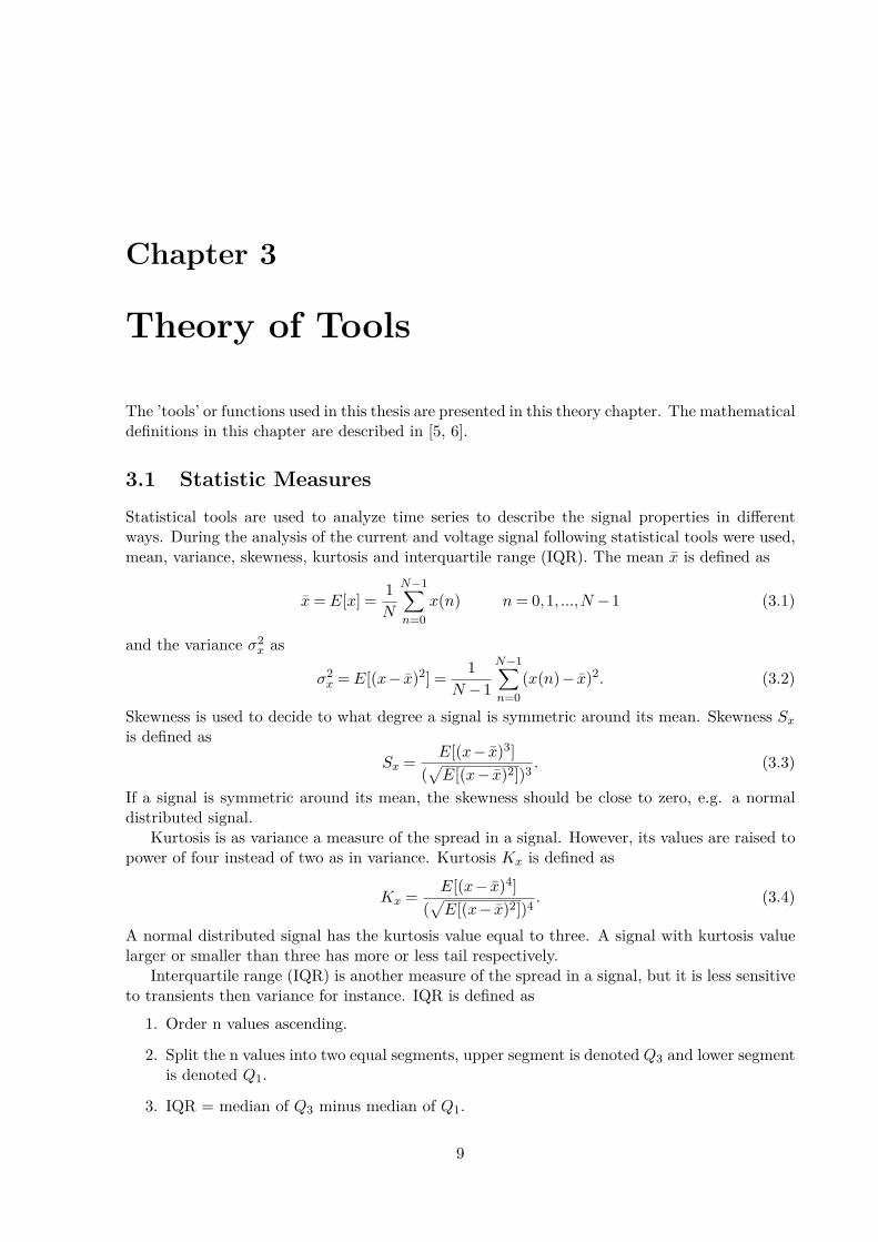
The ’tools’ or functions used in this thesis are presented in this theory chapter. The mathematicaldefinitions in this chapter are described in [5, 6].
3.1 Statistic MeasuresStatistical tools are used to analyze time series to describe the signal properties in differentways. During the analysis of the current and voltage signal following statistical tools were used,mean, variance, skewness, kurtosis and interquartile range (IQR). The mean x is defined as
x= E[x] = 1N
N−1∑
n=0x(n) n= 0,1, ...,N −1 (3.1)
and the variance σ2x as
σ2x =E[(x− x)2] = 1
N −1
N−1∑
n=0(x(n)− x)2. (3.2)
Skewness is used to decide to what degree a signal is symmetric around its mean. Skewness Sxis defined as
Sx = E[(x− x)3](√E[(x− x)2])3 . (3.3)
If a signal is symmetric around its mean, the skewness should be close to zero, e.g. a normaldistributed signal.
Kurtosis is as variance a measure of the spread in a signal. However, its values are raised topower of four instead of two as in variance. Kurtosis Kx is defined as
Kx = E[(x− x)4](√E[(x− x)2])4 . (3.4)
A normal distributed signal has the kurtosis value equal to three. A signal with kurtosis valuelarger or smaller than three has more or less tail respectively.
Interquartile range (IQR) is another measure of the spread in a signal, but it is less sensitiveto transients then variance for instance. IQR is defined as
1. Order n values ascending.
2. Split the n values into two equal segments, upper segment is denoted Q3 and lower segmentis denoted Q1.
3. IQR = median of Q3 minus median of Q1.
9
10 CHAPTER 3. THEORY OF TOOLS
3.2 PeriodogramsPeriodogram methods are used for describing the frequency content of a signal. The use ofdiscrete fourier transform (DFT) on a discrete signal denoted x(n), transforms the x(n) signalinto frequency domain where it is denoted X(k). The DFT is defined as
X(f) =N−1∑
n=0x(n)e−j2πfn 0≤ k ≤N −1 (3.5)
where N is the block length and f = k/N is the frequency. With the use of DFT the standardperiodogram estimate is defined as
Pxx(f) = 2FsN
|X(f)|2 (3.6)
where Fs is the sampling frequency. To minimize leakage among the frequencies a window otherthan the rectangular window should be applied to the discrete signal prior to computing theDTF. The DFT with a window w(n) is defined as
X ′(f) =N−1∑
n=0(w(n)x(n))e−j2πfn 0≤ k ≤N −1 (3.7)
The modified periodogram is defined as
P ′xx(f) = 2FsNB
|X ′(f)|2 (3.8)
where B is window compensation factor. The factor B is defined as
B = 1N
N−1∑
n=0|w(n)|2. (3.9)
To reduce the variance in the periodograms, several periodograms should be averaged. Onemethod that uses this is modified Welch periodogram, which normally also uses overlap betweenblocks to decrease the variance even further, e.g. 50 % or 75%.
To average periodograms the size N is divided into K blocks, each with a length M =N/K.For each block a length M periodogram is calculated and then the K periodograms are averaged.The modified Welch periodogram is defined as
PWxx (f) = 2MLB′
L−1∑
i=0
∣∣∣∣∣M−1∑
n=0(w(n)x(n+ iD))e−j2πfn
∣∣∣∣∣
2
0≤ k ≤M −1 (3.10)
where the length of D controls the overlap percentage and B’ is the window normalization factor.
B′ = 1M
M−1∑
n=0|w(n)|2. (3.11)
3.3 OtherOhms law is a relationship between three variables used the electrical world, and is defined as
U =R · I (3.12)
where U denotes voltage in unit [V]-volt, R denotes resistance in unit [Ω]-Ohm and I denotescurrent in unit [A]-Ampere.
Chapter 4
The Experimental Setup
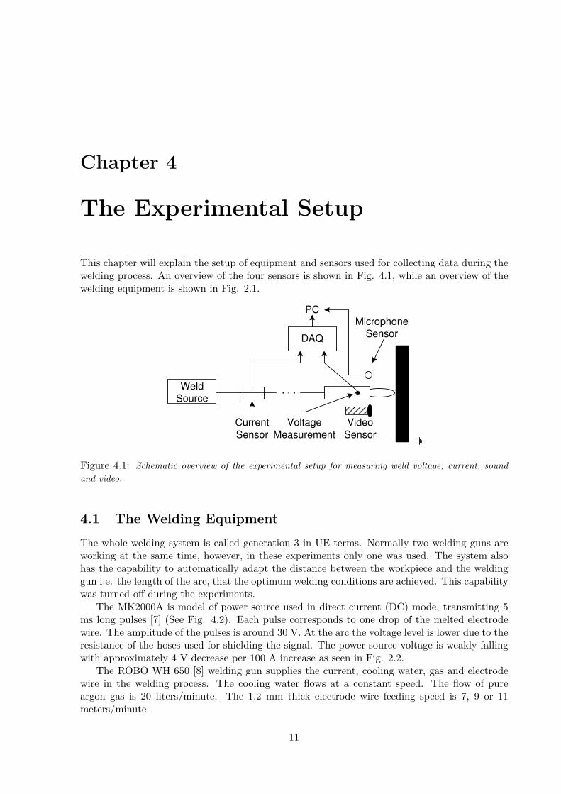
This chapter will explain the setup of equipment and sensors used for collecting data during thewelding process. An overview of the four sensors is shown in Fig. 4.1, while an overview of thewelding equipment is shown in Fig. 2.1.
DAQ
PC
Microphone
Sensor
Weld
Source
Current
Sensor
Voltage
Measurement
. . .
Video
Sensor
Figure 4.1: Schematic overview of the experimental setup for measuring weld voltage, current, soundand video.
4.1 The Welding EquipmentThe whole welding system is called generation 3 in UE terms. Normally two welding guns areworking at the same time, however, in these experiments only one was used. The system alsohas the capability to automatically adapt the distance between the workpiece and the weldinggun i.e. the length of the arc, that the optimum welding conditions are achieved. This capabilitywas turned off during the experiments.
The MK2000A is model of power source used in direct current (DC) mode, transmitting 5ms long pulses [7] (See Fig. 4.2). Each pulse corresponds to one drop of the melted electrodewire. The amplitude of the pulses is around 30 V. At the arc the voltage level is lower due to theresistance of the hoses used for shielding the signal. The power source voltage is weakly fallingwith approximately 4 V decrease per 100 A increase as seen in Fig. 2.2.
The ROBO WH 650 [8] welding gun supplies the current, cooling water, gas and electrodewire in the welding process. The cooling water flows at a constant speed. The flow of pureargon gas is 20 liters/minute. The 1.2 mm thick electrode wire feeding speed is 7, 9 or 11meters/minute.
11
12 CHAPTER 4. THE EXPERIMENTAL SETUP
5ms
3ms
. . .. . .
Time
Voltag
e
Figure 4.2: Pulses generated by the welding power source.
Two different electrode wires were used during the experiments, ESAB OK Autrod 19.82 [9]and Sandvik 29.9 [10]. The chemical composition of the two wires is shown in table 4.1 and 4.2.As seen in tables one is based on nickel while the other is based on iron.
Table 4.2: The chemical composite in percent of wire 29.9.
The electrode wires were mounted in 15 kg bobbins and were fed forward by the rod feederwhich used the pull technique mentioned in Sec. 2.2.3.
4.2. SENSORS 13
4.2 Sensors
In this section sensors used for data collection are presented.
4.2.1 Microphone
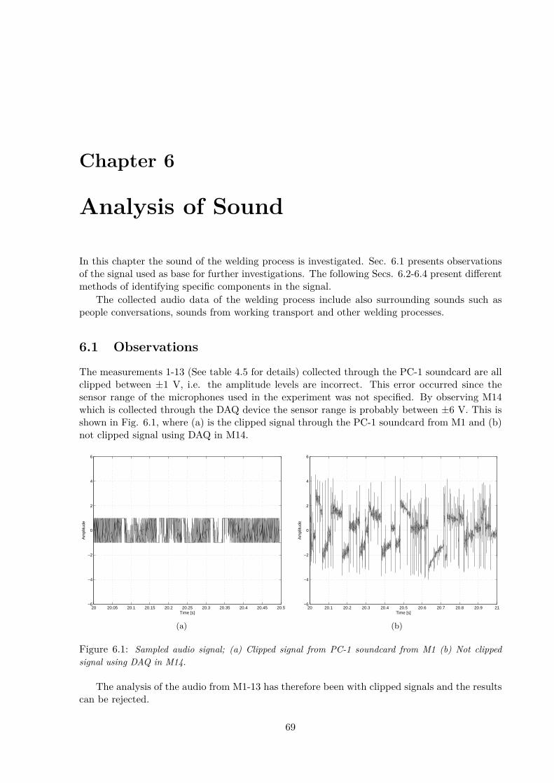
The microphones were installed above the welding gun. The approximately distances betweenthe microphone, welding gun and the arc are shown in the setup Fig. 4.3. The audio signal issampled by the PC builtin soundcard AC97, using its maximum sampling frequency of 44.1 kHzwith 16 bits resolution over the ±1 V range.
DAQ
PC
10cm
30cm
Figure 4.3: Schematic of sound measurement.
During one measurement the Data Acquisition (DAQ) device has been used for recordingthe signal, due to higher sampling frequency possibility. In this measurement two microphonessetup has been used with a sampling frequency of 90 kHz in the limited range of ±10 V.
4.2.2 Current
The current signal was gathered directly after the welding power source by the use of a shunt.In Fig. 4.4 a schematic of the setup is shown.
Weld
Source
OUTPUT
+ - Weld
Workpiece
. . .- +
Figure 4.4: Schematic of current measurement.
A shunt is used since the DAQ measures only voltage. The shunt works as a resistor and itsresistance is only 0.2 mΩ. As the current passes over the shunt, the voltage drop is measuredwith an error accuracy of 0.5 %. An isolation amplifier [11] was used to amplify the signal 100times from 0 - 100 mV to the range of 0 - 10 V. The amplified signal was sampled by the DAQdevice at 44.1 kHz. The amplifier has a maximum delay of 25 ms, which is about 1100 samples.
The measured signal had wrong amplitude levels and was principally wrong type of signali.e. voltage instead of current. However, the signal was reconstructed by dividing of a factor 100and using Ohms law i.e. dividing the signal with the resistance of the shunt. The summarizedfactor is either division by 0.02 or multiplication by 50.
14 CHAPTER 4. THE EXPERIMENTAL SETUP
4.2.3 Voltage
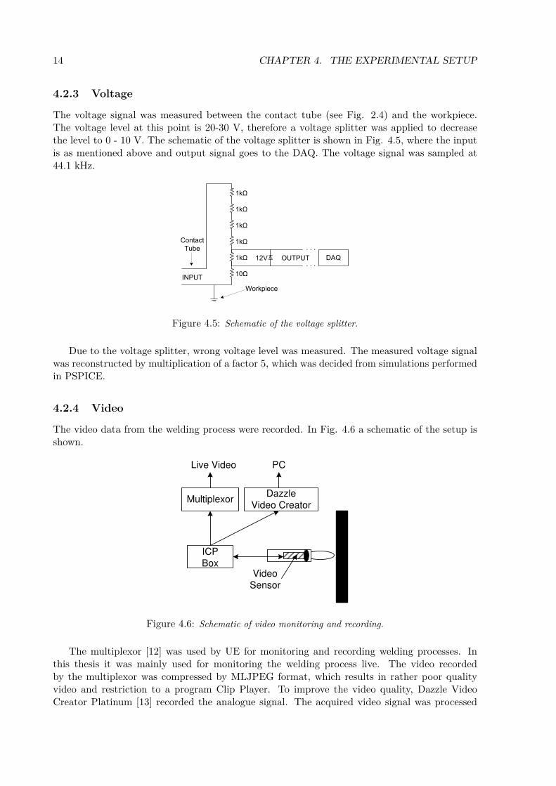
The voltage signal was measured between the contact tube (see Fig. 2.4) and the workpiece.The voltage level at this point is 20-30 V, therefore a voltage splitter was applied to decreasethe level to 0 - 10 V. The schematic of the voltage splitter is shown in Fig. 4.5, where the inputis as mentioned above and output signal goes to the DAQ. The voltage signal was sampled at44.1 kHz.
1k
1k
1k
1k
1k
10
Workpiece
OUTPUT
INPUT
12V
Contact
Tube . . .
. . .DAQ
Figure 4.5: Schematic of the voltage splitter.
Due to the voltage splitter, wrong voltage level was measured. The measured voltage signalwas reconstructed by multiplication of a factor 5, which was decided from simulations performedin PSPICE.
4.2.4 Video
The video data from the welding process were recorded. In Fig. 4.6 a schematic of the setup isshown.
ICP
Box
MultiplexorDazzle
Video Creator
PC
Video
Sensor
Live Video
Figure 4.6: Schematic of video monitoring and recording.
The multiplexor [12] was used by UE for monitoring and recording welding processes. Inthis thesis it was mainly used for monitoring the welding process live. The video recordedby the multiplexor was compressed by MLJPEG format, which results in rather poor qualityvideo and restriction to a program Clip Player. To improve the video quality, Dazzle VideoCreator Platinum [13] recorded the analogue signal. The acquired video signal was processed
4.3. OTHER HARDWARE 15
in Pinnacle Studio version 10. A separate PC was dedicated for recording the video signal inMPEG-4 format.
The camera used is shown in Fig. 4.7, no further information about it can be given due tono reference given from UE.
Figure 4.7: Picture of the fingercamera. The units on the ruler are centimeters.
4.3 Other HardwareOther hardware used during the experiments is explained in this section.
4.3.1 Computers and DAQTwo computers were employed for gathering and storing the signals from the sensors. Detailsabout the computers are listed in table 4.3.
PC-1 PC-2CPU Intel Pentium 1.8GHz Intel Centrino 1.6GHzMemory 1024MB 768MB DDR2 533MHzHDD IDE 120GB 7200RPM IDE 40GB 4200RPMSound AC’97 AC’97
Table 4.3: Specifications of the used computers for collecting and storing sensor information.
NI-9215A [14] DAQ model type was employed to convert the analogous signals to digitalform and temporarily store them. For permanent storage the data were transferred via USB-2.0interface to the PC-1.
The DAQ device has 4 analog input channels, 16 bits of resolution, maximum samplingfrequency of 100 kHz and the analog input range of ±10 V. The experiments setup employsthe range between 0 - 10 V. Specifications of used number of channels and sampling frequencyduring collection data from current and voltage sensors (UA) and from two microphone sensors(UB) are specified in table 4.4.
UA UBChannels 2 2Sampling Frequency [kHz] 44.1 90
Table 4.4: Specifications of used number of channels and sampling frequency when collection data fromcurrent and voltage sensors (UA) and from two microphone sensors (UB).
16 CHAPTER 4. THE EXPERIMENTAL SETUP
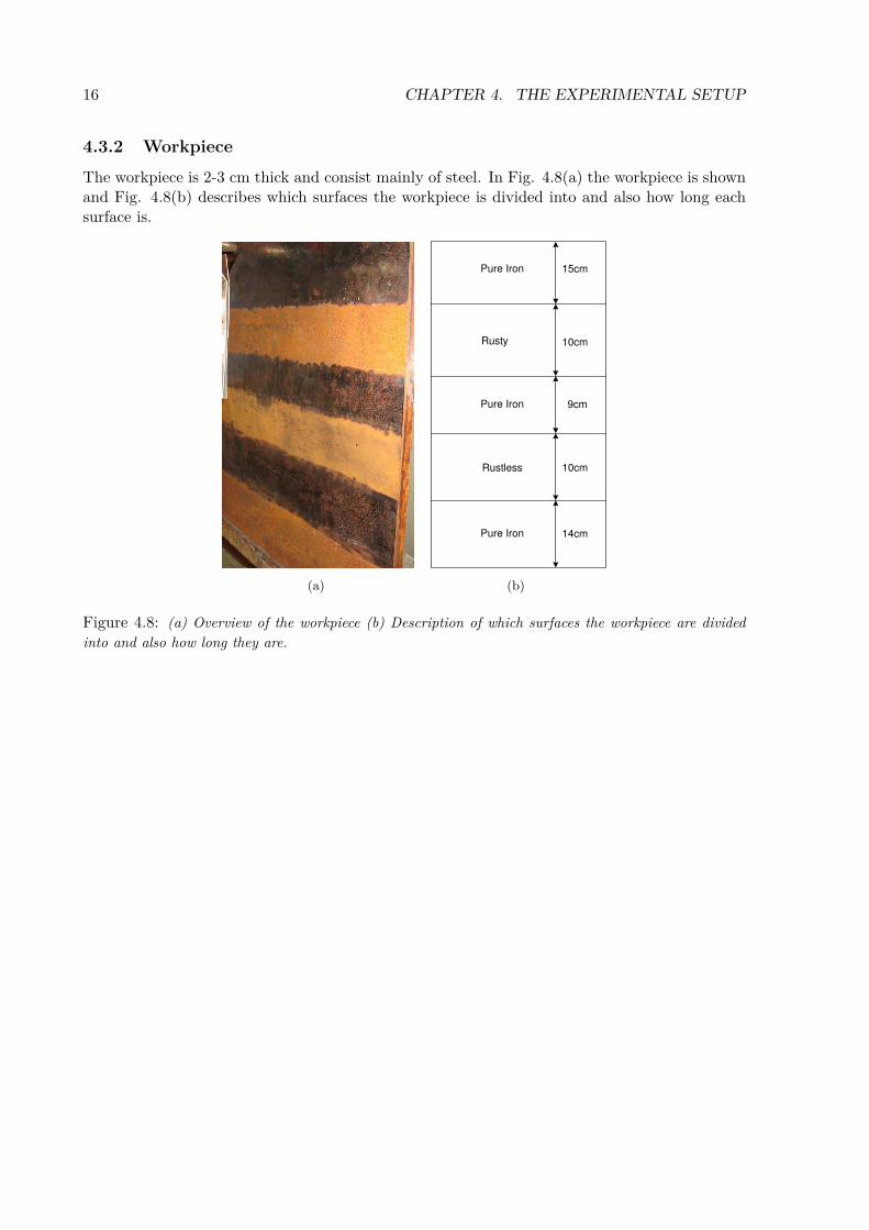
4.3.2 WorkpieceThe workpiece is 2-3 cm thick and consist mainly of steel. In Fig. 4.8(a) the workpiece is shownand Fig. 4.8(b) describes which surfaces the workpiece is divided into and also how long eachsurface is.
(a)
Pure Iron
Rusty
Rustless
Pure Iron
Pure Iron
15cm
10cm
9cm
10cm
14cm
(b)
Figure 4.8: (a) Overview of the workpiece (b) Description of which surfaces the workpiece are dividedinto and also how long they are.
4.4. EXPERIMENTAL PROCEDURE 17
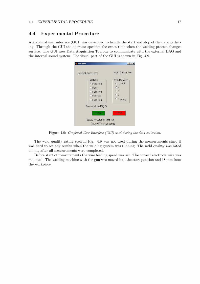
4.4 Experimental ProcedureA graphical user interface (GUI) was developed to handle the start and stop of the data gather-ing. Through the GUI the operator specifies the exact time when the welding process changessurface. The GUI uses Data Acquisition Toolbox to communicate with the external DAQ andthe internal sound system. The visual part of the GUI is shown in Fig. 4.9.
Figure 4.9: Graphical User Interface (GUI) used during the data collection.
The weld quality rating seen in Fig. 4.9 was not used during the measurements since itwas hard to see any results when the welding system was running. The weld quality was ratedoffline, after all measurements were completed.
Before start of measurements the wire feeding speed was set. The correct electrode wire wasmounted. The welding machine with the gun was moved into the start position and 18 mm fromthe workpiece.
18 CHAPTER 4. THE EXPERIMENTAL SETUP
4.5 Visual Welding ResultsTotally 14 measurements were performed, with variated wire speed and different types of elec-trode wires, across five surfaces. Details of each measurement are shown in the table 4.5 andthe results are shown in Figs. 4.10-4.12.
Figure 4.10: Visual welding results from measurements 4-9. The upper numbers indicate with electrodewire type used and the lower numbers are the wire speed [m/min].
29.9 19.82
9117 79 11
Figure 4.11: Visual welding results from measurements 1-3 and 10-12. The upper numbers indicate withelectrode wire type used and the lower numbers are the wire speed [m/min].
In this chapter the measured current and voltage signals are investigated. Sec. 5.1 and 5.2 areseen as introduction to the signals properties and Sec. 5.3 to 5.5 present different methods foremploying the weld data to monitoring welding process.
The different measurements presented in Sec. 4.1, are from now on referenced as e.g. M1 formeasurement 1. The M1 corresponds to the first two welded surfaces with wire feeding speedof 9 m/min using electrode wire 29.9, see table 4.5. Another definition used for now on is, goodand bad surface. Good corresponds to pure iron surface and bad corresponds to either a rustyor rustless surfaces.
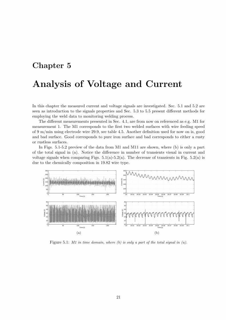
In Figs. 5.1-5.2 preview of the data from M1 and M11 are shown, where (b) is only a partof the total signal in (a). Notice the difference in number of transients visual in current andvoltage signals when comparing Figs. 5.1(a)-5.2(a). The decrease of transients in Fig. 5.2(a) isdue to the chemically composition in 19.82 wire type.
Figure 5.1: M1 in time domain, where (b) is only a part of the total signal in (a).
21
22 CHAPTER 5. ANALYSIS OF VOLTAGE AND CURRENT
0 50 100 150 2000
50
100
150
200
250
300
Time [s]
Cur
rent
[A]
0 50 100 150 2000
10
20
30
40
50
60
Time [s]
Vol
tage
[V]
(a)
20.52 20.54 20.56 20.58 20.6 20.62 20.64110
120
130
140
150
160
Time [s]
Cur
rent
[A]
20.52 20.54 20.56 20.58 20.6 20.62 20.6410
15
20
25
30
35
40
Time [s]
Vol
tage
[V]
(b)
Figure 5.2: M11 in time domain, where (b) is only a part of the total signal in (a).
5.1 Stationarity & NormalityThis section is divided into two subsections, voltage 5.1.1 and current 5.1.2. Each subsectionis divided into three paragraphs to overview the results. The theory of these paragraphs ispresented below.
1. Investigation of signal’s stationarity is performed with suitable block size. It will be per-formed by calculating mean and variance over the five surfaces. The expected outcome ofthis method should either have lowpass or highpass filter characteristics. These tests areperformed on M1, M5, M8 and M11 with the block sizes given in table 5.1, where upperrow is the true size and lower row is the number seen in Fig 5.3-5.4 and 5.7-5.8.
Table 5.1: Upper row is the true size and lower row is the number seen in Figs. 5.3-5.4 and 5.7-5.8.
2. With the chosen block size frame statistics and reversed arrangement tests will be applied.
3. Determine if the signals are normal(Gaussian) distributed or not.
5.1. STATIONARITY & NORMALITY 23
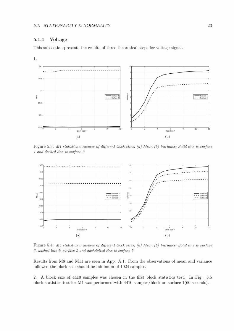
5.1.1 VoltageThis subsection presents the results of three theoretical steps for voltage signal.
1.
0 2 4 6 8 10 1223.85
23.9
23.95
24
24.05
24.1
Block Size #
Mea
n
Surface 1Surface 2
(a)
0 2 4 6 8 10 120
1
2
3
4
5
6
7
8
9
10
Block Size #
Var
ianc
e
Surface 1Surface 2
(b)
Figure 5.3: M1 statistics measures of different block sizes; (a) Mean (b) Variance; Solid line is surface1 and dashed line is surface 2.
0 2 4 6 8 10 1224.5
24.55
24.6
24.65
24.7
24.75
24.8
24.85
24.9
24.95
Block Size #
Mea
n
Surface 3Surface 4Surface 5
(a)
0 2 4 6 8 10 120
1
2
3
4
5
6
7
8
Block Size #
Var
ianc
e
Surface 3Surface 4Surface 5
(b)
Figure 5.4: M5 statistics measures of different block sizes; (a) Mean (b) Variance; Solid line is surface3, dashed line is surface 4 and dashdotted line is surface 5.
Results from M8 and M11 are seen in App. A.1. From the observations of mean and variancefollowed the block size should be minimum of 1024 samples.
2. A block size of 4410 samples was chosen in the first block statistics test. In Fig. 5.5block statistics test for M1 was performed with 4410 samples/block on surface 1(60 seconds).
24 CHAPTER 5. ANALYSIS OF VOLTAGE AND CURRENT
0 100 200 300 400 50022
22.5
23
23.5
24
24.5
25
25.5
Block #
Mea
n
(a)
0 100 200 300 400 5000
5
10
15
20
25
30
35
40
45
Block #
Var
ianc
e
(b)
Figure 5.5: Block statistics test for stationarity with 4410 samples/block on surface 1(60 seconds) inM1; (a) Mean (b) Variance.
The mean and variance in Fig. 5.5 vary between 22.5-25.3 and 3.5-44.4 respectively. It isclearly seen that the signal is non-stationary. This is most likely due to the random narrowspikes (transients) in the data.
To verify the result, the reversed arrangement test was used with same data and block sizeusing significant value α= 0.05. Both mean and variance were found to be non-stationary.
3. The histograms from M1 and M11 are shown in Figs. 5.6(a)-5.6(b). The skewness are-2.8 and -2.4 for M1 and M11 respectively, which states that they are clearly not normally dis-tributed. This is verified by kurtosis measure. M1 and M11 produces 15.1 and 10.6 which isabove normal kurtosis value.
0 10 20 30 40 50 600
2
4
6
8
10
12x 10
4
data
# of
eve
nts
(a)
0 10 20 30 40 50 600
2
4
6
8
10
12
14x 10
4
data
# of
eve
nts
(b)
Figure 5.6: Histogram of (a) M1 (b) M11.
5.1. STATIONARITY & NORMALITY 25
5.1.2 CurrentThis subsection presents the results of three theoretical steps for current signal.
1.
0 2 4 6 8 10 12135.5
136
136.5
137
137.5
138
138.5
139
139.5
140
Block Size #
Mea
n
Surface 1Surface 2
(a)
0 2 4 6 8 10 120
10
20
30
40
50
60
70
80
90
100
Block Size #
Var
ianc
e
Surface 1Surface 2
(b)
Figure 5.7: M1 statistics measures of different block sizes; (a) Mean (b) Variance; Solid line is surface1 and dashed line is surface 2.
0 2 4 6 8 10 12124
125
126
127
128
129
130
131
132
133
Block Size #
Mea
n
Surface 3Surface 4Surface 5
(a)
0 2 4 6 8 10 120
10
20
30
40
50
60
70
80
90
Block Size #
Var
ianc
e
Surface 3Surface 4Surface 5
(b)
Figure 5.8: M5 statistics measures of different block sizes; (a) Mean (b) Variance; Solid line is surface3, dashed line is surface 4 and dashdotted line is surface 5.
Results from M8 and M11 are seen in App. A.2. From the observations of mean and variancefollowed the block size should be minimum of 256 samples.
2. A block size of 4410 samples was chosen in the first block statistics test. In Fig. 5.9block statistics test for M1 was performed with 4410 samples/block on surface 1(60 seconds).
26 CHAPTER 5. ANALYSIS OF VOLTAGE AND CURRENT
0 100 200 300 400 500115
120
125
130
135
140
145
150
155
160
Block #
Mea
n
(a)
0 100 200 300 400 5000
100
200
300
400
500
600
700
800
900
Block #
Var
ianc
e
(b)
Figure 5.9: Block statistics test for stationarity with 4410 samples/block on surface 1(60 seconds) inM1; (a) Mean (b) Variance.
The mean and variance in Fig. 5.9 vary between 116-160 and 7-860 respectively. It is seenthat the signal is not stationary. This is most likely due to the random narrow spikes (transients)in the data.
To verify the result, the reversed arrangement test was used with same data and block size us-ing significant value α= 0.05. The mean was found as non-stationary, but variance as stationary.
3. The histograms from M1 and M11 are shown in Figs. 5.10(a)-5.10(b). The skewness are-3.6 and -2.9 for M1 and M11 respectively, which states that they are clearly not normally dis-tributed. This is verified by kurtosis measure. M1 and M11 produces 19.7 and 12.2 which isabove normal kurtosis value.
0 50 100 150 200 2500
1
2
3
4
5
6
7x 10
4
data
# of
eve
nts
(a)
20 40 60 80 100 120 140 160 180 200 2200
1
2
3
4
5
6
7
8
9x 10
4
data
# of
eve
nts
(b)
Figure 5.10: Histogram of (a) M1 (b) M11.
5.2. OBSERVATIONS 27
5.2 ObservationsThe 29.9 and 19.82 wires are considered as good and bad respectively. Wire feeding speed at 9m/min is considered as normal speed, therefore are 7 m/min and 11 m/min considered as lowand high respectively.
In Figs. 4.10-4.12 the visual results of the welding measurements are shown. In M1 and M5(normal wire speed) the welding results are the best and obtain the highest grade even if thereare a few small holes. High wire speed provides better results than low speed, in comparisonM3, M4, M9 and M10 with M2, M6, M7 and M12.
In M2 and M6 the surfaces are colored red, due to the chemical composite in the 29.9 wirerunning at a low speed. Outcome from both wires has different shades, which has to do withthe chemical composites.
How do the above mentioned results behave in the gathered data series, when entering a badsurface? In general the mean and skewness increases while variance and kurtosis decreases forvoltage. For the current signal these conclusions are the opposite.
When running at higher wire speed the current level is increased. It is because of the strongrelationship between the wire speed and current. At higher speed, the current flows through thewire for a less time than at a lower speed and therefore the heat in the wire is lower. It leadsto lowered resistance in the wire. Hence, voltage in the arc increases and the welding currentincreases.
By examining the current data, the welding row change can easily be detected, since that occursrepeatedly about every other second. The characteristic in the current changes very rapidly forwire speeds of 9 and 11 m/min, which are shown in Figs. 5.11-5.13(a) that are for M1, M2and M3. This behavior might also be detected in the voltage data, but not as easy as with thecurrent.
25 26 27 28 29 30 31 32 33 34 35100
110
120
130
140
150
160
170
180
190
200
Time[s]
Cur
rent
[A]
(a)
25 26 27 28 29 30 31 32 33 34 350
10
20
30
40
50
60
Time[s]
Vol
tage
[V]
(b)
Figure 5.11: M1; (a) shows the current data with the rapidly changing characteristic when switchingrow in welding process; (b) shows the voltage and it’s transients.
28 CHAPTER 5. ANALYSIS OF VOLTAGE AND CURRENT
25 26 27 28 29 30 31 32 33 34 3560
70
80
90
100
110
120
130
140
150
160
Time[s]
Cur
rent
[A]
(a)
25 26 27 28 29 30 31 32 33 34 350
10
20
30
40
50
60
Time[s]
Vol
tage
[V]
(b)
Figure 5.12: M1; (a) shows the current data with the rapidly changing characteristic when switchingrow in welding process; (b) shows the voltage and it’s transients.
25 26 27 28 29 30 31 32 33 34 35100
150
200
250
Time[s]
Cur
rent
[A]
(a)
25 26 27 28 29 30 31 32 33 34 350
10
20
30
40
50
60
Time[s]
Vol
tage
[V]
(b)
Figure 5.13: M1; (a) shows the current data with the rapidly changing characteristic when switchingrow in welding process; (b) shows the voltage and it’s transients.
The number of high level spikes (transients) seen mainly in the voltage data, increases withincreased wire speed. Generally the amount of transients decreases on a bad surface withinconsistencies at the low wire speed. In Figs. 5.11-5.13(b) this behavior is shown. The lowernumber of transients in data from the bad surfaces can indicate as limited penetration in theworkpiece.
5.3. METHOD 1: SPECTROGRAMS 29
5.3 Method 1: SpectrogramsThis method is based on how the signals behave in the frequency domain. Spectrograms areused to show how the frequency content changes over time, i.e. as the welding process contin-ues. The estimation of the power spectrum (PS) is based on the modified periodograms method[5]. The data series are divided into block length 4096 samples, using 4096 FFT points for thecalculating the PS estimate. Prior to computing the periodogram a hanning window is appliedto lower the spectral leakage in each block.
The method is divided into three parts.
1. Make and investigate spectrograms.
2. Identify area of interest and build filters.
3. Run a program that filters the signal and calculate statistical data to monitor the weldingprocess.
Each of these steps is presented for voltage and current in subsections 5.3.1 and 5.3.2 respec-tively.
5.3.1 Voltage1. In Figs. 5.14-5.19 spectrograms for M1, M2, M3, M10, M11 and M12 are shown using a blocklength of 4096 samples and 4096 FFT points.
Figure 5.14: Spectrogram of M1.
30 CHAPTER 5. ANALYSIS OF VOLTAGE AND CURRENT
Figure 5.15: Spectrogram of M2.
Figure 5.16: Spectrogram of M3.
5.3. METHOD 1: SPECTROGRAMS 31
Figure 5.17: Spectrogram of M10. Notice the change of surfaces at 1500 and 2500 blocks.
Figure 5.18: Spectrogram of M11.
32 CHAPTER 5. ANALYSIS OF VOLTAGE AND CURRENT
Figure 5.19: Spectrogram of M12.
2. In Figs. 5.14-5.16 (M1, M2, M3) no significant difference is observed between the twosurfaces. However, in Figs. 5.17-5.19 (M10, M11, M12) some difference is observed. Notice thatM10 enters a third surface as well (Fig. 5.17).
The main differences occur above 400 Hz which is second harmonic and up to 22050 Hz(Fs/2). There are numerous harmonics below 3-4 kHz. Therefore the area of interest is definedbetween 3-4 kHz and Fs/2. A highpass filter with elliptic characteristics was designed, see Fig.5.20.
0 0.5 1 1.5 2
x 104
−150
−100
−50
0
Mag
nitu
de [d
B]
Frequency [Hz]
0 0.5 1 1.5 2
x 104
−150
−100
−50
0
50
100
150
Pha
se [D
egre
es]
Frequency [Hz]
Figure 5.20: Designed highpass filter for voltage.
5.3. METHOD 1: SPECTROGRAMS 33
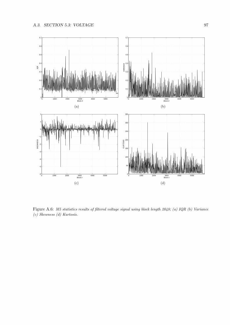
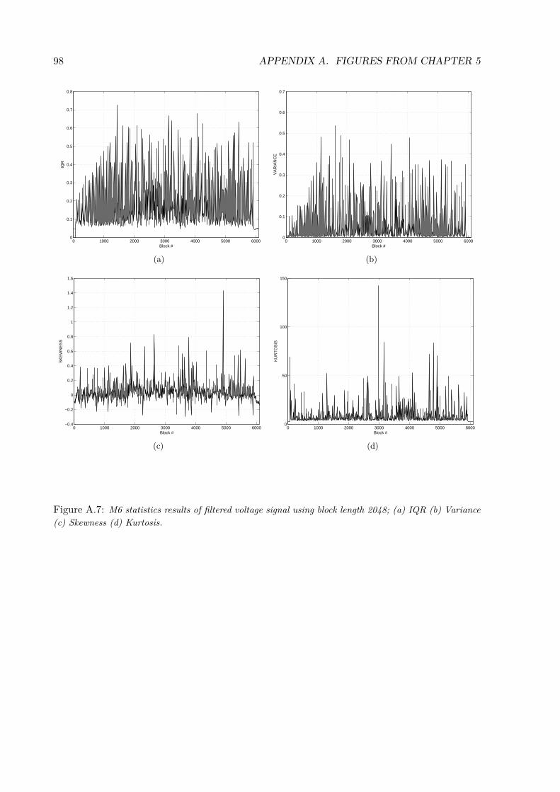
3. The data is filtered with the designed highpass filter and divided into blocks of a predefinedlength. Iqr, mean, variance, skewness and kurtosis statistics are calculated.
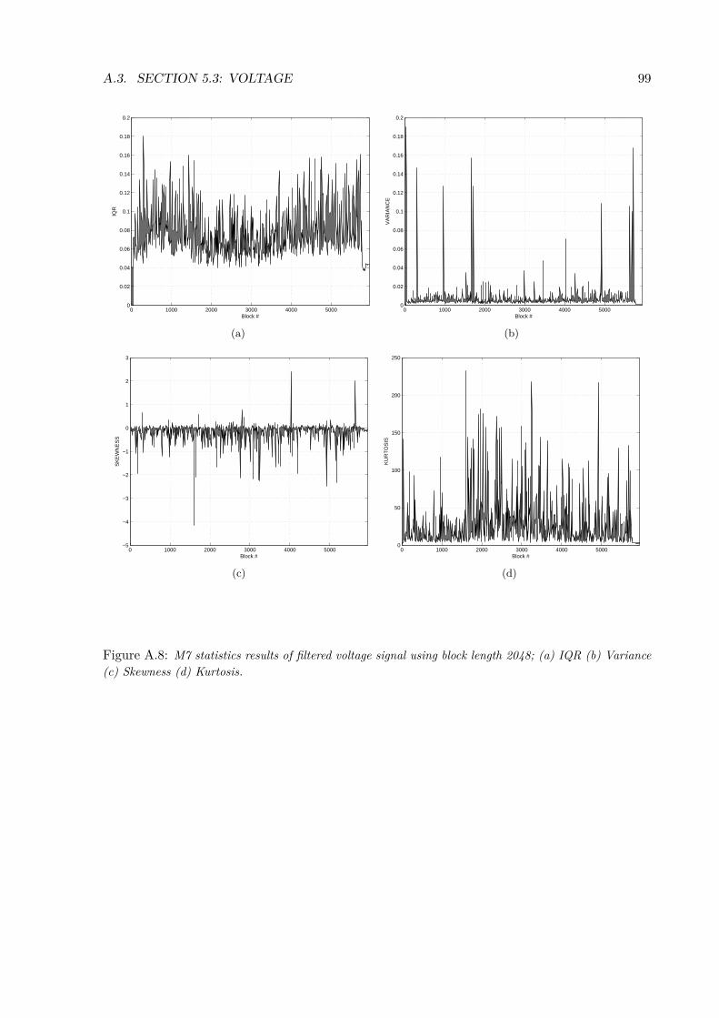
The following results were obtained by smoothing 7 blocks with 2048 samples each. Theoutcomes for M1, M2, M3, M10, M11 and M12 are shown in Figs. 5.21-5.26. For more resultssee App. A.3.
0 500 1000 1500 2000 2500 3000 3500 4000 45000
0.05
0.1
0.15
0.2
0.25
0.3
0.35
0.4
0.45
Block #
IQR
(a)
0 500 1000 1500 2000 2500 3000 3500 4000 45000
0.1
0.2
0.3
0.4
0.5
0.6
0.7
Block #
VA
RIA
NC
E
(b)
0 500 1000 1500 2000 2500 3000 3500 4000 4500−4
−3
−2
−1
0
1
2
Block #
SK
EW
NE
SS
(c)
0 500 1000 1500 2000 2500 3000 3500 4000 45000
50
100
150
200
250
Block #
KU
RT
OS
IS
(d)
Figure 5.21: M1 statistics results of filtered voltage signal using block length 2048; (a) IQR (b) Variance(c) Skewness (d) Kurtosis.
34 CHAPTER 5. ANALYSIS OF VOLTAGE AND CURRENT
0 500 1000 1500 2000 2500 3000 3500 4000 45000
0.1
0.2
0.3
0.4
0.5
0.6
0.7
Block #
IQR
(a)
0 500 1000 1500 2000 2500 3000 3500 4000 45000
0.05
0.1
0.15
0.2
0.25
0.3
0.35
0.4
0.45
Block #
VA
RIA
NC
E
(b)
0 500 1000 1500 2000 2500 3000 3500 4000 4500−0.6
−0.4
−0.2
0
0.2
0.4
0.6
0.8
1
1.2
Block #
SK
EW
NE
SS
(c)
0 500 1000 1500 2000 2500 3000 3500 4000 45000
10
20
30
40
50
60
70
80
Block #
KU
RT
OS
IS
(d)
Figure 5.22: M2 statistics results of filtered voltage signal using block length 2048; (a) IQR (b) Variance(c) Skewness (d) Kurtosis.
5.3. METHOD 1: SPECTROGRAMS 35
0 500 1000 1500 2000 2500 3000 3500 4000 45000
0.05
0.1
0.15
0.2
0.25
0.3
0.35
0.4
0.45
0.5
Block #
IQR
(a)
0 500 1000 1500 2000 2500 3000 3500 4000 45000
0.1
0.2
0.3
0.4
0.5
0.6
0.7
0.8
0.9
1
Block #
VA
RIA
NC
E
(b)
0 500 1000 1500 2000 2500 3000 3500 4000 4500−2.5
−2
−1.5
−1
−0.5
0
0.5
1
1.5
Block #
SK
EW
NE
SS
(c)
0 500 1000 1500 2000 2500 3000 3500 4000 45000
20
40
60
80
100
120
140
Block #
KU
RT
OS
IS
(d)
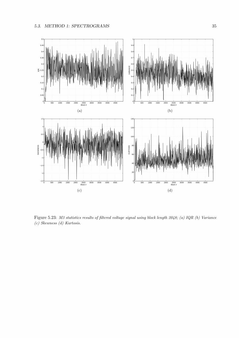
Figure 5.23: M3 statistics results of filtered voltage signal using block length 2048; (a) IQR (b) Variance(c) Skewness (d) Kurtosis.
36 CHAPTER 5. ANALYSIS OF VOLTAGE AND CURRENT
0 1000 2000 3000 4000 50000
0.05
0.1
0.15
0.2
0.25
0.3
0.35
0.4
0.45
Block #
IQR
(a)
0 1000 2000 3000 4000 50000
0.1
0.2
0.3
0.4
0.5
0.6
0.7
0.8
Block #
VA
RIA
NC
E
(b)
0 1000 2000 3000 4000 5000−4
−3
−2
−1
0
1
2
Block #
SK
EW
NE
SS
(c)
0 1000 2000 3000 4000 50000
50
100
150
200
250
300
Block #
KU
RT
OS
IS
(d)
Figure 5.24: M10 statistics results of filtered voltage signal using block length 2048; (a) IQR (b) Variance(c) Skewness (d) Kurtosis.
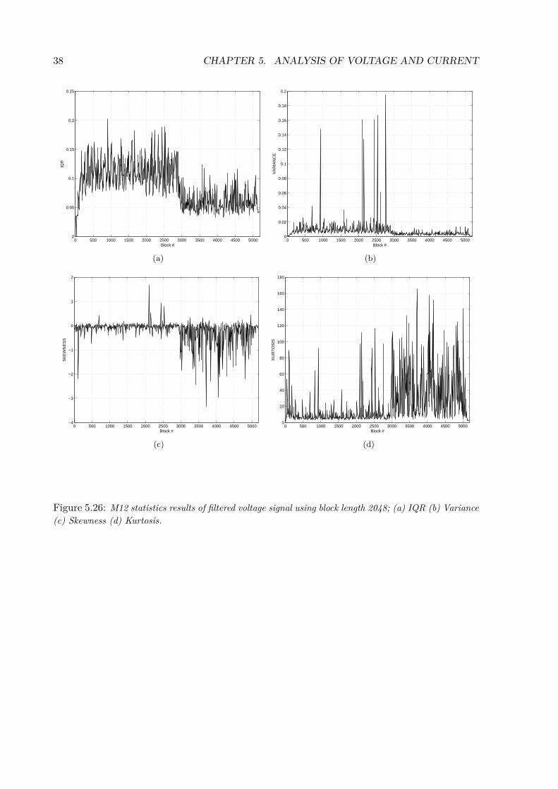
Figure 5.26: M12 statistics results of filtered voltage signal using block length 2048; (a) IQR (b) Variance(c) Skewness (d) Kurtosis.
5.3. METHOD 1: SPECTROGRAMS 39
5.3.2 Current1. The current data are concentrated in low frequency band which is shown in Fig. 5.27. InFigs. 5.28-5.33 spectrograms for M1, M2, M3, M10, M11 and M12 are shown using a blocklength of 2048 samples and 4096 FFT points. each of these measurements is downsampled witha factor five from a sampling frequency of 44.1 kHz to 8820 Hz, however, is limited between 0- 2 kHz in the figures. It is downsampled to increase the actual FFT points in that frequencyrange which increases the visibility. In Fig. 5.27 there is one FFT point per 11 Hz and in Figs.5.28-5.33 one FFT point per 2 Hz.
Figure 5.27: Spectrogram of M1 over whole spectrum.
40 CHAPTER 5. ANALYSIS OF VOLTAGE AND CURRENT
Figure 5.28: Spectrogram of M1.
Figure 5.29: Spectrogram of M2.
5.3. METHOD 1: SPECTROGRAMS 41
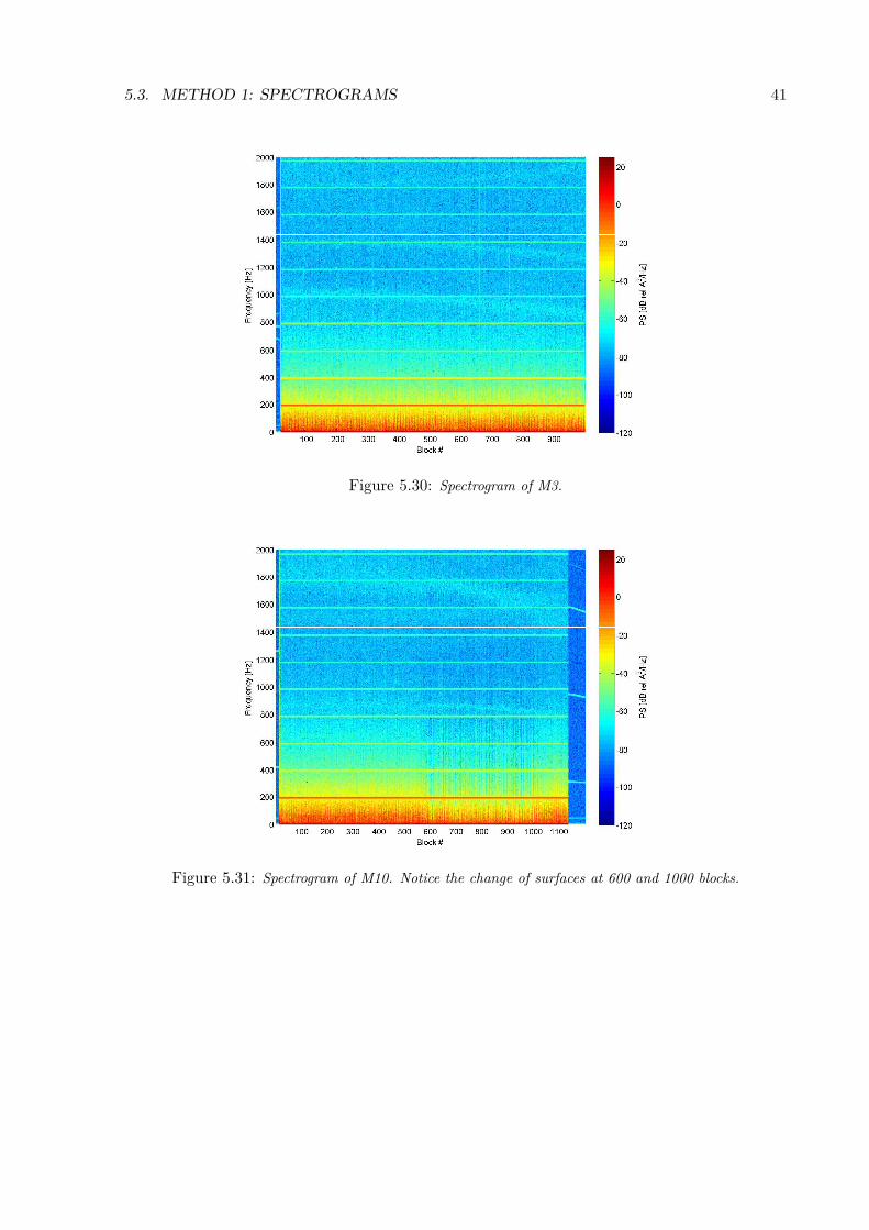
Figure 5.30: Spectrogram of M3.
Figure 5.31: Spectrogram of M10. Notice the change of surfaces at 600 and 1000 blocks.
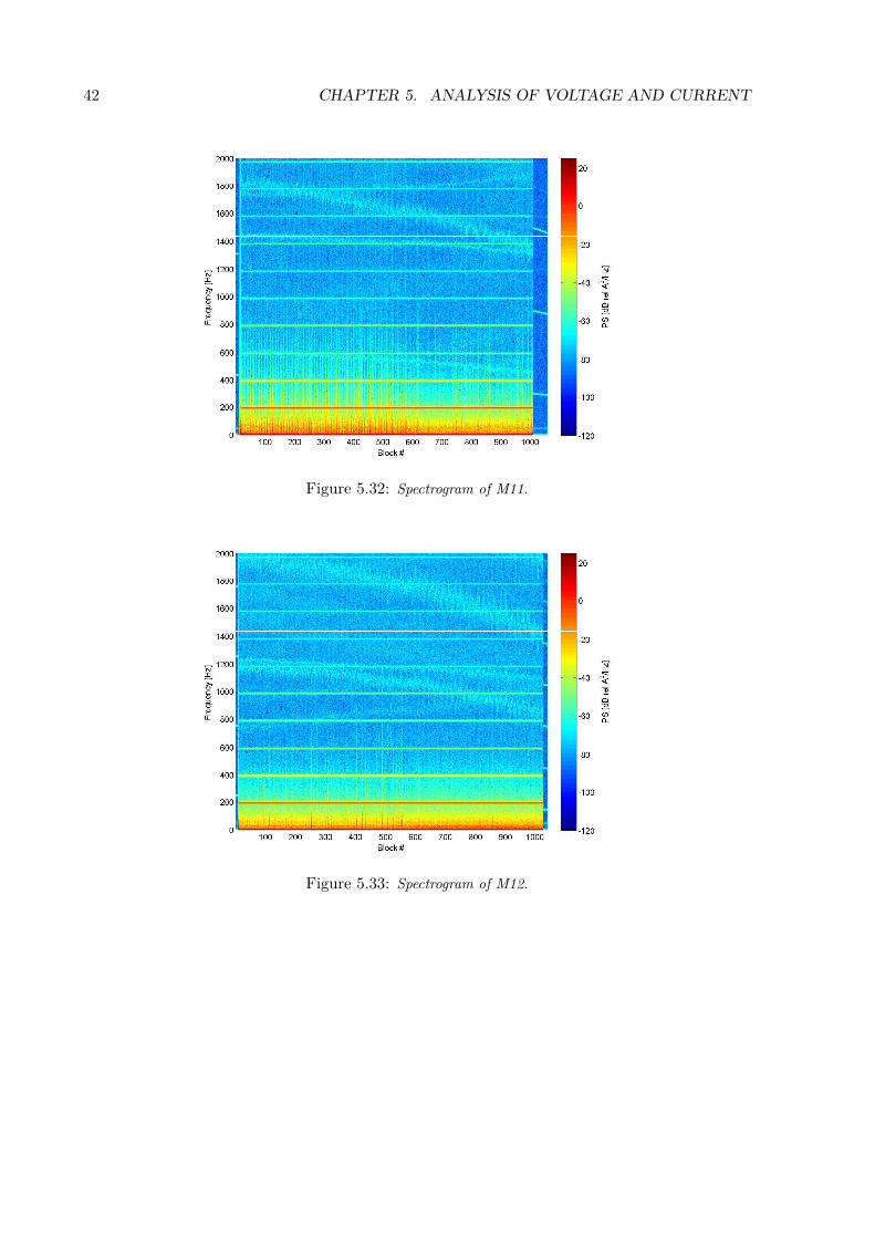
42 CHAPTER 5. ANALYSIS OF VOLTAGE AND CURRENT
Figure 5.32: Spectrogram of M11.
Figure 5.33: Spectrogram of M12.
5.3. METHOD 1: SPECTROGRAMS 43
2. In Figs. 5.28-5.30 (M1, M2, M3) no significant difference is observed between the surfaces.However, in Figs. 5.31-5.33 (M10, M11, M12) some difference is noticed. Notice that M10 entersa third surface aswell.
Since the main differences occur between 100 - 1000 Hz, the area of interest is defined in thisfrequency band. A lowpass filter with butterworth characteristics was designed, see Fig. 5.34.
0 500 1000 1500 2000 2500 3000 3500 4000−150
−100
−50
0M
agni
tude
[dB
]
Frequency [Hz]
0 500 1000 1500 2000 2500 3000 3500 4000
−150
−100
−50
0
50
100
150
Pha
se [D
egre
es]
Frequency [Hz]
Figure 5.34: Designed lowpass filter for current.
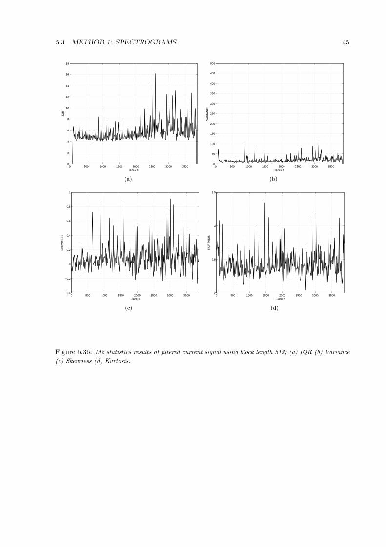
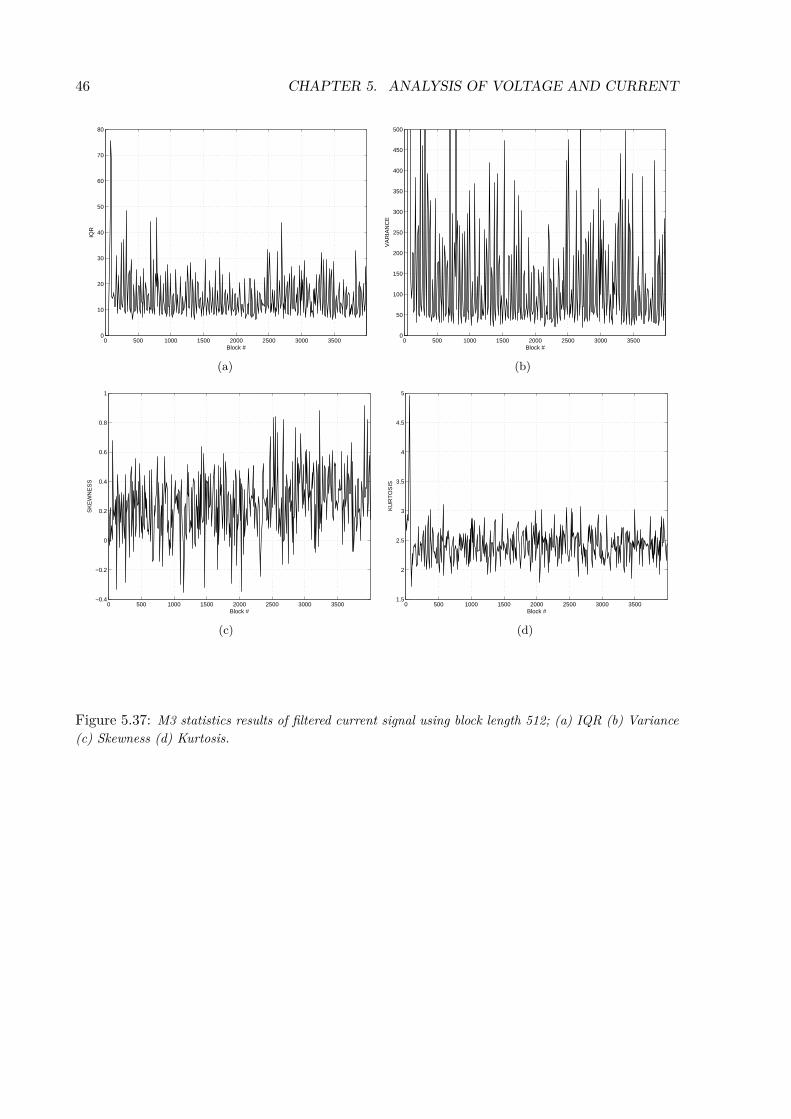
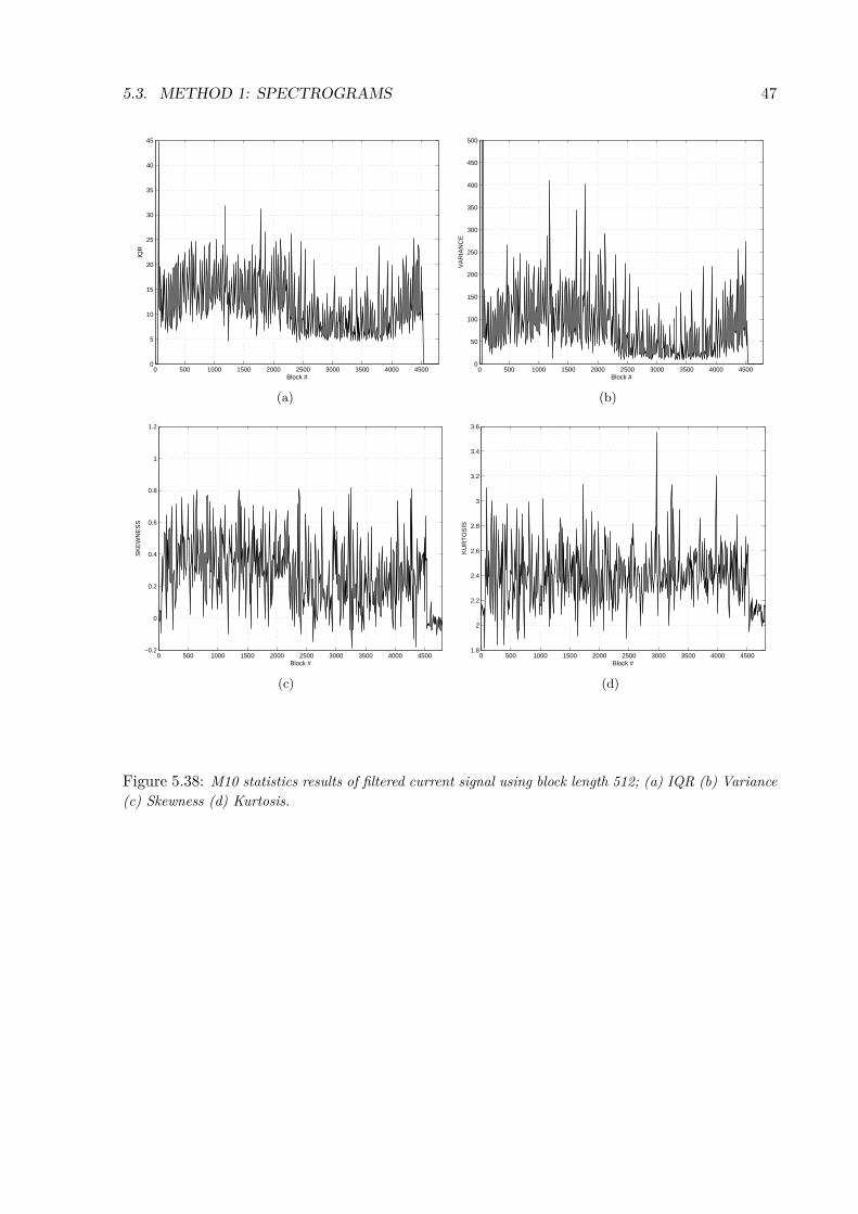
3. The data is downsampled by a factor 5, filtered with the designed lowpass filter and di-vided into blocks of predefined length. Iqr, mean, variance, skewness and kurtosis statistics arecalculated.
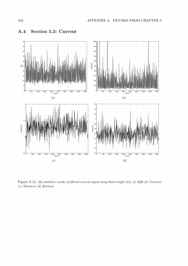
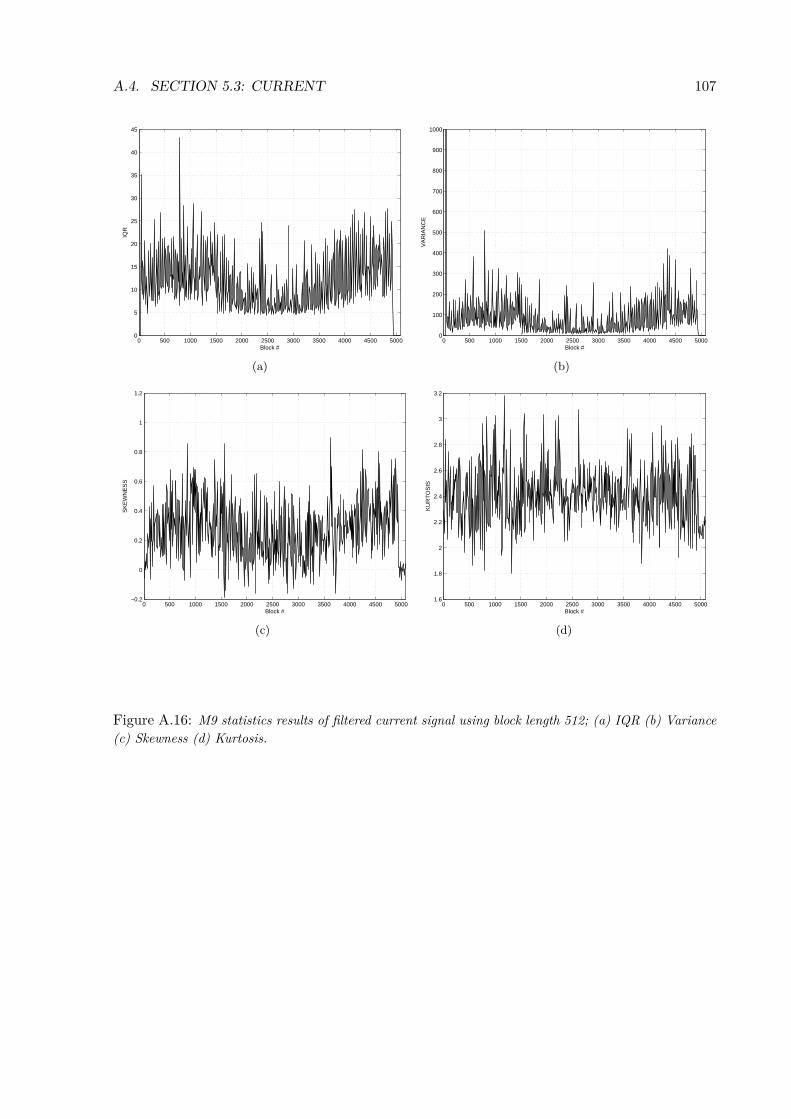
The following results were obtained by smoothing 9 blocks with 512 samples each. Theoutcomes for M1, M2, M3, M10, M11 and M12 are shown in Figs. 5.35-5.40. For more resultssee App. A.4.
44 CHAPTER 5. ANALYSIS OF VOLTAGE AND CURRENT
0 500 1000 1500 2000 2500 3000 35000
10
20
30
40
50
60
70
80
Block #
IQR
(a)
0 500 1000 1500 2000 2500 3000 35000
50
100
150
200
250
300
350
400
450
500
Block #
VA
RIA
NC
E
(b)
0 500 1000 1500 2000 2500 3000 3500−0.8
−0.6
−0.4
−0.2
0
0.2
0.4
0.6
0.8
1
Block #
SK
EW
NE
SS
(c)
0 500 1000 1500 2000 2500 3000 35001.8
2
2.2
2.4
2.6
2.8
3
3.2
3.4
3.6
Block #
KU
RT
OS
IS
(d)
Figure 5.35: M1 statistics results of filtered current signal using block length 512; (a) IQR (b) Variance(c) Skewness (d) Kurtosis.
5.3. METHOD 1: SPECTROGRAMS 45
0 500 1000 1500 2000 2500 3000 35000
2
4
6
8
10
12
14
16
18
Block #
IQR
(a)
0 500 1000 1500 2000 2500 3000 35000
50
100
150
200
250
300
350
400
450
500
Block #
VA
RIA
NC
E
(b)
0 500 1000 1500 2000 2500 3000 3500−0.4
−0.2
0
0.2
0.4
0.6
0.8
1
Block #
SK
EW
NE
SS
(c)
0 500 1000 1500 2000 2500 3000 35002
2.5
3
3.5
Block #
KU
RT
OS
IS
(d)
Figure 5.36: M2 statistics results of filtered current signal using block length 512; (a) IQR (b) Variance(c) Skewness (d) Kurtosis.
46 CHAPTER 5. ANALYSIS OF VOLTAGE AND CURRENT
0 500 1000 1500 2000 2500 3000 35000
10
20
30
40
50
60
70
80
Block #
IQR
(a)
0 500 1000 1500 2000 2500 3000 35000
50
100
150
200
250
300
350
400
450
500
Block #
VA
RIA
NC
E
(b)
0 500 1000 1500 2000 2500 3000 3500−0.4
−0.2
0
0.2
0.4
0.6
0.8
1
Block #
SK
EW
NE
SS
(c)
0 500 1000 1500 2000 2500 3000 35001.5
2
2.5
3
3.5
4
4.5
5
Block #
KU
RT
OS
IS
(d)
Figure 5.37: M3 statistics results of filtered current signal using block length 512; (a) IQR (b) Variance(c) Skewness (d) Kurtosis.
5.3. METHOD 1: SPECTROGRAMS 47
0 500 1000 1500 2000 2500 3000 3500 4000 45000
5
10
15
20
25
30
35
40
45
Block #
IQR
(a)
0 500 1000 1500 2000 2500 3000 3500 4000 45000
50
100
150
200
250
300
350
400
450
500
Block #
VA
RIA
NC
E
(b)
0 500 1000 1500 2000 2500 3000 3500 4000 4500−0.2
0
0.2
0.4
0.6
0.8
1
1.2
Block #
SK
EW
NE
SS
(c)
0 500 1000 1500 2000 2500 3000 3500 4000 45001.8
2
2.2
2.4
2.6
2.8
3
3.2
3.4
3.6
Block #
KU
RT
OS
IS
(d)
Figure 5.38: M10 statistics results of filtered current signal using block length 512; (a) IQR (b) Variance(c) Skewness (d) Kurtosis.
48 CHAPTER 5. ANALYSIS OF VOLTAGE AND CURRENT
0 500 1000 1500 2000 2500 3000 3500 40000
20
40
60
80
100
120
140
Block #
IQR
(a)
0 500 1000 1500 2000 2500 3000 3500 40000
50
100
150
200
250
300
350
400
450
500
Block #
VA
RIA
NC
E
(b)
0 500 1000 1500 2000 2500 3000 3500 4000−0.6
−0.4
−0.2
0
0.2
0.4
0.6
0.8
1
1.2
1.4
Block #
SK
EW
NE
SS
(c)
0 500 1000 1500 2000 2500 3000 3500 40001.5
2
2.5
3
3.5
4
4.5
Block #
KU
RT
OS
IS
(d)
Figure 5.39: M11 statistics results of filtered current signal using block length 512; (a) IQR (b) Variance(c) Skewness (d) Kurtosis.
5.3. METHOD 1: SPECTROGRAMS 49
0 500 1000 1500 2000 2500 3000 3500 40000
1
2
3
4
5
6
7
8
9
10
Block #
IQR
(a)
0 500 1000 1500 2000 2500 3000 3500 40000
50
100
150
200
250
300
350
400
450
500
Block #
VA
RIA
NC
E
(b)
0 500 1000 1500 2000 2500 3000 3500 4000−0.5
−0.4
−0.3
−0.2
−0.1
0
0.1
0.2
0.3
Block #
SK
EW
NE
SS
(c)
0 500 1000 1500 2000 2500 3000 3500 40002
2.5
3
3.5
Block #
KU
RT
OS
IS
(d)
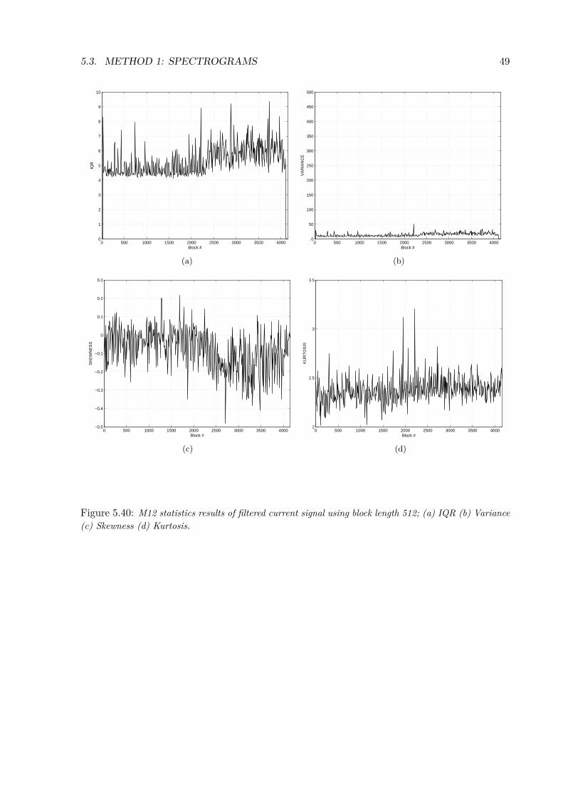
Figure 5.40: M12 statistics results of filtered current signal using block length 512; (a) IQR (b) Variance(c) Skewness (d) Kurtosis.
50 CHAPTER 5. ANALYSIS OF VOLTAGE AND CURRENT
5.3.3 SummaryThe modified spectrogram can detect when the welding changes from a clean good surface, i.e.stainless steel surface to a bad surface containing a rusty layer. The voltage signal shows theclearest difference. Variance and iqr are two strong tools in detection of surface change. In somecases even mean, skewness and kurtosis are also good tools to use.
The method has some disadvantages
• Small differences are hard to observe. For example in the end of M1, there are severalsmall holes which are hard to detect.
• The probability of false alarms might be high due to presence of spikes.
• If the welding quality is low from the beginning, it would probably not be detected untilthe quality of the weld changes.
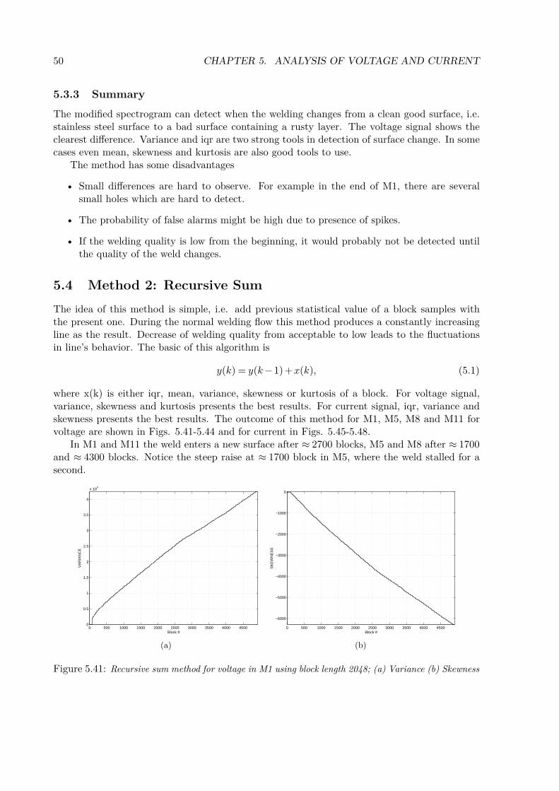
5.4 Method 2: Recursive SumThe idea of this method is simple, i.e. add previous statistical value of a block samples withthe present one. During the normal welding flow this method produces a constantly increasingline as the result. Decrease of welding quality from acceptable to low leads to the fluctuationsin line’s behavior. The basic of this algorithm is
y(k) = y(k−1)+x(k), (5.1)
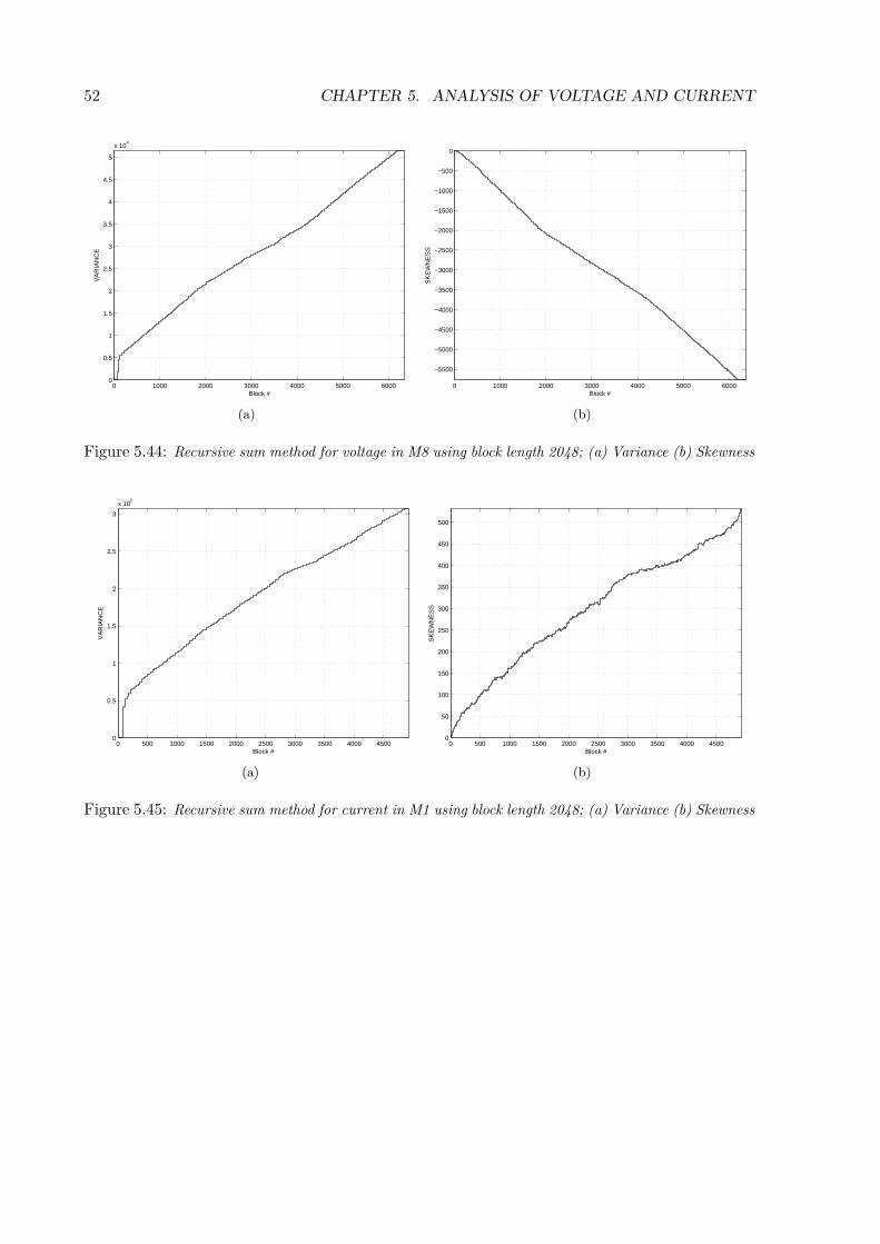
where x(k) is either iqr, mean, variance, skewness or kurtosis of a block. For voltage signal,variance, skewness and kurtosis presents the best results. For current signal, iqr, variance andskewness presents the best results. The outcome of this method for M1, M5, M8 and M11 forvoltage are shown in Figs. 5.41-5.44 and for current in Figs. 5.45-5.48.
In M1 and M11 the weld enters a new surface after ≈ 2700 blocks, M5 and M8 after ≈ 1700and ≈ 4300 blocks. Notice the steep raise at ≈ 1700 block in M5, where the weld stalled for asecond.
0 500 1000 1500 2000 2500 3000 3500 4000 45000
0.5
1
1.5
2
2.5
3
3.5
4
x 104
Block #
VA
RIA
NC
E
(a)
0 500 1000 1500 2000 2500 3000 3500 4000 4500
−6000
−5000
−4000
−3000
−2000
−1000
0
Block #
SK
EW
NE
SS
(b)
Figure 5.41: Recursive sum method for voltage in M1 using block length 2048; (a) Variance (b) Skewness
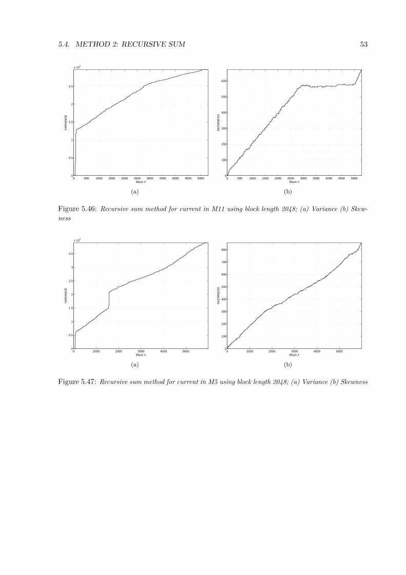
Figure 5.46: Recursive sum method for current in M11 using block length 2048; (a) Variance (b) Skew-ness
0 1000 2000 3000 4000 50000
0.5
1
1.5
2
2.5
3
3.5
x 105
Block #
VA
RIA
NC
E
(a)
0 1000 2000 3000 4000 50000
100
200
300
400
500
600
700
800
Block #
SK
EW
NE
SS
(b)
Figure 5.47: Recursive sum method for current in M5 using block length 2048; (a) Variance (b) Skewness
54 CHAPTER 5. ANALYSIS OF VOLTAGE AND CURRENT
0 1000 2000 3000 4000 5000 60000
0.5
1
1.5
2
2.5
3
x 105
Block #
VA
RIA
NC
E
(a)
0 1000 2000 3000 4000 5000 60000
100
200
300
400
500
600
Block #
SK
EW
NE
SS
(b)
Figure 5.48: Recursive sum method for current in M8 using block length 2048; (a) Variance (b) Skewness
The method defined in Eq. (5.1) can generally monitor the welding process. Welding undernormal conditions should produce a straight growing line. If one or several of the conditionschange the angle of the growing line also change. In our case the surface factor changes betweena good and bad surface.
The idea is good for a general overview, however, it cannot detect small errors in the weld,expressed by the holes in the new layer.
After introducing a forgetting term γ to Eq. (5.1) the outcome of algorithm becomes com-pletely different.
y(k) = γ ·y(k−1)+x(k) 0 γ < 1 (5.2)
With the given equation and normal wire speed, i.e. 9 m/min, the detection of small holes orerrors is simplified. If the wire speed is 7 or 11 m/min the results are harder to interpret. 7m/min produces bad weld on even good surfaces. 11 m/min because of high number of transientsproduces inaccuracy in this algorithm.
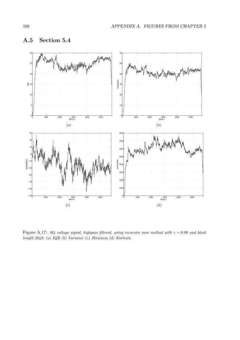
The results of applying this algorithm with block length 2048 and γ = 0.99 on the voltagesignal for M1 and M5 are shown in Figs. 5.49-5.50. Results for M4 are shown in Fig. 5.51 tosupport that high wire speed are harder to interpret. Notice that the x-axis shows row numbersinstead of block numbers and arrows are added in the areas of interest for easier comparisonwith Figs. 4.10-4.11.
5.4. METHOD 2: RECURSIVE SUM 55
0 20 40 60 80 100300
305
310
315
320
325
330
335
340
345
350
Row #
INT
ER
QU
AR
TIL
E R
AN
GE
(a)
0 20 40 60 80 100400
600
800
1000
1200
1400
1600
Row #
VA
RIA
NC
E
(b)
0 20 40 60 80 100
−180
−170
−160
−150
−140
−130
−120
−110
−100
−90
Row #
SK
EW
NE
SS
(c)
0 20 40 60 80 100300
400
500
600
700
800
900
1000
Row #
KU
RT
OS
IS
(d)
Figure 5.49: Recursive sum method with forgetting factor γ = 0.99, voltage in M1 using block length2048; (a) IQR (b) Variance (c) Skewness (d) Kurtosis.
56 CHAPTER 5. ANALYSIS OF VOLTAGE AND CURRENT
0 20 40 60 80 100 120310
320
330
340
350
360
370
Row #
INT
ER
QU
AR
TIL
E R
AN
GE
(a)
0 20 40 60 80 100 120500
600
700
800
900
1000
1100
Row #
VA
RIA
NC
E
(b)
0 20 40 60 80 100 120−140
−130
−120
−110
−100
−90
−80
−70
−60
Row #
SK
EW
NE
SS
(c)
0 20 40 60 80 100 120300
350
400
450
500
550
600
650
700
750
800
Row #
KU
RT
OS
IS
(d)
Figure 5.50: Recursive sum method with forgetting factor γ = 0.99, voltage in M5 using block length2048; (a) IQR (b) Variance (c) Skewness (d) Kurtosis.
5.4. METHOD 2: RECURSIVE SUM 57
0 20 40 60 80 100 120400
450
500
550
600
650
700
Row #
INT
ER
QU
AR
TIL
E R
AN
GE
(a)
0 20 40 60 80 100 1201500
2000
2500
3000
3500
4000
4500
Row #
VA
RIA
NC
E
(b)
0 20 40 60 80 100 120−180
−170
−160
−150
−140
−130
−120
−110
−100
Row #
SK
EW
NE
SS
(c)
0 20 40 60 80 100 120500
550
600
650
700
750
800
850
900
Row #
KU
RT
OS
IS
(d)
Figure 5.51: Recursive sum method with forgetting factor γ = 0.99, voltage in M4 using block length2048; (a) IQR (b) Variance (c) Skewness (d) Kurtosis.
58 CHAPTER 5. ANALYSIS OF VOLTAGE AND CURRENT
5.4.1 SummaryTwo methods were presented in this section. The first one was more general overview of thewelding process while the second one aimed on the details of the weld.
The first method with overview capability might be seen as monitoring the stability of theprocess and can perhaps easily detect changes in the process. It cannot in any way detect smallerrors, such as holes created by the bad weld.
The second method with aim on details of the data for locating holes, errors or unevennesson the surfaces seems to work satisfactory. With some further testing on more data series withthe normal wire type (29.9), it’s capabilities might be fully explored and understood. In currentstate the method shows a few false alarm, i.e. peaks in the results of the algorithm that cannotbe found by looking at the surface.
5.5 Method: Recursive Sum Combined with Filter MethodThis section presents a combined method of the spectrograms and the recursive sum. The appli-cation of these two methods together has a significant impact on the outcome of the algorithm.The results for voltage signal for M1, M2, M3, M10, M11 and M10 are shown in Figs. 5.52-5.57,for further results see App. A.5. Block length was set to 2048, no smoothing and the forgettingfactor was 0.99.
5.5. METHOD: RECURSIVE SUM COMBINED WITH FILTER METHOD 59
0 500 1000 1500 2000 2500 3000 3500 4000 45000
5
10
15
20
25
Block #
IQR
(a)
0 500 1000 1500 2000 2500 3000 3500 4000 45000
5
10
15
20
25
30
35
Block #
VA
RIA
NC
E
(b)
0 500 1000 1500 2000 2500 3000 3500 4000 4500−100
−80
−60
−40
−20
0
20
Block #
SK
EW
NE
SS
(c)
0 500 1000 1500 2000 2500 3000 3500 4000 45000
2000
4000
6000
8000
10000
12000
Block #
KU
RT
OS
IS
(d)
Figure 5.52: M1 voltage signal, highpass filtered, using recursive sum method with γ = 0.99 and blocklength 2048; (a) IQR (b) Variance (c) Skewness (d) Kurtosis.
60 CHAPTER 5. ANALYSIS OF VOLTAGE AND CURRENT
0 500 1000 1500 2000 2500 3000 3500 4000 45000
5
10
15
20
25
30
Block #
IQR
(a)
0 500 1000 1500 2000 2500 3000 3500 4000 45000
5
10
15
Block #
VA
RIA
NC
E
(b)
0 500 1000 1500 2000 2500 3000 3500 4000 4500−25
−20
−15
−10
−5
0
5
10
15
20
25
Block #
SK
EW
NE
SS
(c)
0 500 1000 1500 2000 2500 3000 3500 4000 45000
500
1000
1500
2000
2500
3000
3500
Block #
KU
RT
OS
IS
(d)
Figure 5.53: M2 voltage signal, highpass filtered, using recursive sum method with γ = 0.99 and blocklength 2048; (a) IQR (b) Variance (c) Skewness (d) Kurtosis.
5.5. METHOD: RECURSIVE SUM COMBINED WITH FILTER METHOD 61
0 500 1000 1500 2000 2500 3000 3500 4000 45000
5
10
15
20
25
30
35
Block #
IQR
(a)
0 500 1000 1500 2000 2500 3000 3500 4000 45000
10
20
30
40
50
60
Block #
VA
RIA
NC
E
(b)
0 500 1000 1500 2000 2500 3000 3500 4000 4500−60
−50
−40
−30
−20
−10
0
10
20
30
Block #
SK
EW
NE
SS
(c)
0 500 1000 1500 2000 2500 3000 3500 4000 45000
1000
2000
3000
4000
5000
6000
7000
8000
Block #
KU
RT
OS
IS
(d)
Figure 5.54: M3 voltage signal, highpass filtered, using recursive sum method with γ = 0.99 and blocklength 2048; (a) IQR (b) Variance (c) Skewness (d) Kurtosis.
62 CHAPTER 5. ANALYSIS OF VOLTAGE AND CURRENT
0 1000 2000 3000 4000 50000
5
10
15
20
25
30
Block #
IQR
(a)
0 1000 2000 3000 4000 50000
5
10
15
20
25
30
35
40
45
50
Block #
VA
RIA
NC
E
(b)
0 1000 2000 3000 4000 5000−100
−80
−60
−40
−20
0
20
Block #
SK
EW
NE
SS
(c)
0 1000 2000 3000 4000 50000
1000
2000
3000
4000
5000
6000
7000
8000
9000
10000
Block #
KU
RT
OS
IS
(d)
Figure 5.55: M10 voltage signal, highpass filtered, using recursive sum method with γ = 0.99 and blocklength 2048; (a) IQR (b) Variance (c) Skewness (d) Kurtosis.
5.5. METHOD: RECURSIVE SUM COMBINED WITH FILTER METHOD 63
Figure 5.57: M12 voltage signal, highpass filtered, using recursive sum method with γ = 0.99 and blocklength 2048; (a) IQR (b) Variance (c) Skewness (d) Kurtosis.
5.5. METHOD: RECURSIVE SUM COMBINED WITH FILTER METHOD 65
5.5.1 DecimationUntil now all calculations for voltage signal were using the original sampling frequency (Fs) of44.1 kHz. Precision is lost by decimating the number of samples per second. In this sectionthe precision of the algorithm used in Sec. 5.5 is affected due to the decimation. It is shown inFig. 5.59 (Fs = 22050 Hz) and 5.60 (Fs = 14700 Hz). Notice Fig. 5.58(Fs = 44100 Hz) is notdecimated by any factor.
0 500 1000 1500 2000 2500 3000 3500 4000 45000
5
10
15
20
25
Block #
IQR
(a)
0 500 1000 1500 2000 2500 3000 3500 4000 45000
5
10
15
20
25
30
35
Block #
VA
RIA
NC
E
(b)
Figure 5.58: M1 voltage signal, highpass filtered, using recursive sum method with γ = 0.99 and blocklength 2048; (a) IQR (b) Variance.
66 CHAPTER 5. ANALYSIS OF VOLTAGE AND CURRENT
0 500 1000 1500 20000
2
4
6
8
10
12
14
Block #
IQR
(a)
0 500 1000 1500 20000
2
4
6
8
10
12
14
16
18
Block #
VA
RIA
NC
E
(b)
Figure 5.59: M1 voltage signal, decimated by 2, highpass filtered, using recursive sum method withγ = 0.99 and block length 2048; (a) IQR (b) Variance.
0 200 400 600 800 1000 1200 1400 16000
1
2
3
4
5
6
7
8
9
10
Block #
IQR
(a)
0 200 400 600 800 1000 1200 1400 16000
1
2
3
4
5
6
7
Block #
VA
RIA
NC
E
(b)
Figure 5.60: M1 voltage signal, decimated by 3, highpass filtered, using recursive sum method withγ = 0.99 and block length 2048; (a) IQR (b) Variance.
The effect of lowering the sampling frequency is insignificant. The sampling frequency couldprobably be reduced to 22 kHz without any greater loss of precision.
5.5.2 SummaryThe combined method of the filter method and the recursive sum provides better results thantheir separate application. The good and bad surfaces are still clearly separated to see a differ-ence in the results, where variance and iqr are the strongest tools.
The details for small errors, i.e. indication of holes on the welded surface, are not lost invariance and iqr results. However, the interpretation of the skewness and kurtosis results is moredifficult. If the weld starts on a bad surface and produces poor quality weld, the algorithm canperhaps only detect the problem when the process gets better. It is therefore essential to makethe assumption that the weld starts on a good surface and produces normal quality weld.
5.6. SUMMARY 67
In subsection 5.5.1 the effect of lowering the sampling frequency was shown. It was demon-strated that the sampling frequency could be halved without making any radical changes in theresults.
5.6 Summary
From the results shown in this chapter we now know that separation of the good and bad sur-faces is possible. However, detection of small areas of bad weld on any surfaces is and shallbe hard to make robust in any future detection algorithm. During welding on a bad surfacethe probability of producing bad weld is higher than on a good surface. This means when thewelding passes a bad surface, the algorithm will show a big dip and the operator notes that areaas possible bad weld.
From [6, 15] many good ideas for solving the detection problem originated. A few of them arepresented in this chapter. The algorithm based on Sequential Probability Ratio Test (SPRT)presented in [15] and further developed in [16] have been extensively tested. It did not produceany results worth presenting in this thesis. However, both references state that this specificSPRT algorithm was only built for short-arc welding.
In the first two sections properties and observations were stated. Both current and voltagesignal were non-stationary processes, most likely because of the transients observed in the data.The mean and skewness increase while variance, iqr and kurtosis decrease when entering a badsurface. In general when holes occur in the weld the statistics properties mentioned above be-come the opposite, e.g. skewness suddenly decreases. Note that when using wire speeds at 7 or11 m/min these properties might be shifted.
In the third section the data were presented in frequency domain vs time domain in spec-trograms. The investigations of the frequency content reveal that the band between 3-4 kHzand Fs/2 shows the most noticeable change of the voltage signal. The current signal changessignificantly in the frequency band between 0 Hz and 1 kHz. The statistical properties wereobtained from filtered signals. The result from this section was not very promising, however, asstated before, variance and iqr show the biggest difference between the surfaces.
In the fourth section two alternative versions of the recursive sum method were presented.Without any forgetting factor, the method was suitable for monitoring the stability of the
welding system. While the curve is a straight line the process is normal. When the curve changesangle something has changed, e.g. bad surface as in this thesis. In real world system it could beused to robustly detect changes in the gas and wire flow.
With forgetting factor the method improved the visual perception of differences betweensurfaces. It is possible to identify the positions of the bad welding occurrence due to suddenjump in the method’s outcome. Results from this method was shown for M1, M3 and M5, sincethe wire speed of 9 m/min (normal) is of main interest.
In the fifth section, the combined method between filter method and the recursive sum methodwas presented. The combination of these methods resulted into a better visual difference be-tween surfaces. The details that show the occurrence of bad weld within the different surfacesremained as in the filter method and the recursive sum method.
A test of lowering the sampling frequency on the voltage was also performed. The test
68 CHAPTER 5. ANALYSIS OF VOLTAGE AND CURRENT
indicated the sampling frequency can be decreased down to 20 kHz. In Sec. 5.3 it was alsodemonstrated that the sampling frequency for current signal can be reduced below 10 kHzwithout significant loss of information. The combined method was the final method presentedin this chapter.
Chapter 6
Analysis of Sound
In this chapter the sound of the welding process is investigated. Sec. 6.1 presents observationsof the signal used as base for further investigations. The following Secs. 6.2-6.4 present differentmethods of identifying specific components in the signal.
The collected audio data of the welding process include also surrounding sounds such aspeople conversations, sounds from working transport and other welding processes.
6.1 Observations
The measurements 1-13 (See table 4.5 for details) collected through the PC-1 soundcard are allclipped between ±1 V, i.e. the amplitude levels are incorrect. This error occurred since thesensor range of the microphones used in the experiment was not specified. By observing M14which is collected through the DAQ device the sensor range is probably between ±6 V. This isshown in Fig. 6.1, where (a) is the clipped signal through the PC-1 soundcard from M1 and (b)not clipped signal using DAQ in M14.
Figure 6.1: Sampled audio signal; (a) Clipped signal from PC-1 soundcard from M1 (b) Not clippedsignal using DAQ in M14.
The analysis of the audio from M1-13 has therefore been with clipped signals and the resultscan be rejected.
69
70 CHAPTER 6. ANALYSIS OF SOUND
The true observations of the signal can be obtained with proper choice of tools. By analyzingthe whole signal between 0 - 22050 Hz, the sound can generally be divided into two groups, highand low frequencies.
The low frequency group is between 0 - 4 kHz, where a clear sound is heard. The sound laststwo seconds followed by a short break and is continuously repeated in this matter. The intervalof the sound is of the same length as the sound produced by the machine movement. However,it can also be produced from the arc. This frequency band also includes the human voices andnumerous of repeated sounds which might be produced by screeching from the bobbin deviceand the welding machine itself.
The high frequency group is above 4 kHz where most of the spatter sounds from the weldare present and probably a large number sounds produced by the arc.
The wire speed has strong influence on sounds amplitude. At low wire speed (7m/min) moreof the low frequency group is heard, at high wire speed (11m/min) less of the low frequencygroup is heard. The normal wire speed (9m/min) is somewhere in between the two groups. Thiscan directly be compared with the data collected from the voltage signal. It has low number oftransients (high frequency) with low wire speed and high number of transients with high wirespeed.
There are no clear audibly differences with use of 29.9 wire type. Perhaps a small audibledifference when using the 19.82 wire type. With the use of spectrograms, a visual differencebetween a pure iron and rusty surface can be shown, mainly during use of wire type 19.82.In Figs. 6.2-6.3 spectrograms of M3 and M12 are shown respectively, using block size of 4096samples and 4096 FFT points.
Figure 6.2: Spectrogram of M3. At ≈ 1500 blocks the welding process proceeds on the rusty surface.
6.2. METHOD 1: RECURSIVE SUM 71
Figure 6.3: Spectrogram of M12. At ≈ 1500 blocks the welding process proceeds on the rusty surface.
6.2 Method 1: Recursive SumFrom the spectrograms shown in Figs. 6.2-6.3 a main difference is shown above 3-4 kHz. Thefrequency bandwidth of interest is therefore chosen from 3-4 kHz upto 22.05 kHz. A 7th orderIIR highpass filter with elliptic characteristics was designed. In MATLAB ellipord and ellipfunctions was used. The designed filter is shown in Fig. 6.4.
0 0.5 1 1.5 2
x 104
−150
−100
−50
0
Mag
nitu
de [d
B]
Frequency [Hz]
0 0.5 1 1.5 2
x 104
−150
−100
−50
0
50
100
150
Pha
se [D
egre
es]
Frequency [Hz]
Figure 6.4: Designed highpass filter for sound.
72 CHAPTER 6. ANALYSIS OF SOUND
The filtered audio signals from M1 and M11 are seen in Fig. 6.5. Notice the significantdifference in Fig. 6.5(b) in amplitude after filtered the signal compared to Fig. 6.5(a). At ≈ 130blocks the welding process proceeds on the rusty surface.
0 50 100 150 200−2.5
−2
−1.5
−1
−0.5
0
0.5
1
1.5
2
2.5
Time [s]
Am
plitu
de
(a)
0 50 100 150 200−2.5
−2
−1.5
−1
−0.5
0
0.5
1
1.5
2
2.5
Time [s]
Am
plitu
de
(b)
Figure 6.5: Highpass filtered sound signal in time domain; (a) M1 (b) M11
The definition of the recursive sum method using a forgetting factor is shown in Eq. (5.2),where γ is chosen to 0.99. In the previous experiments statistical tools measuring the spread inthe signal have proven to produce the best results. Therefore in this experiment only varianceand kurtosis are applied. The block size is 4096. The results of applying this method on M1,M2, M3, M10, M11, M12 and M13 are shown in Figs. 6.6-6.12. For more information see App.B.1.
0 500 1000 1500 20000
5
10
15
20
25
Block #
VA
RIA
NC
E
(a)
0 500 1000 1500 20000
50
100
150
200
250
300
350
400
450
500
Block #
KU
RT
OS
IS
(b)
Figure 6.6: Highpass filtered M1 sound signal, using recursive sum method with γ = 0.99 and blocklength 4096; (a) Variance (b) Kurtosis. At ≈ 1500 blocks the welding proceeds on the rusty surface.
6.2. METHOD 1: RECURSIVE SUM 73
0 500 1000 1500 20000
5
10
15
20
25
30
35
Block #
VA
RIA
NC
E
(a)
0 500 1000 1500 20000
50
100
150
200
250
300
350
400
Block #
KU
RT
OS
IS
(b)
Figure 6.7: Highpass filtered M2 sound signal, using recursive sum method with γ = 0.99 and block length4096; (a) Variance (b) Kurtosis. At ≈ 1500 blocks the welding process proceeds on the rusty surface.
0 500 1000 1500 20000
5
10
15
20
25
Block #
VA
RIA
NC
E
(a)
0 500 1000 1500 20000
100
200
300
400
500
600
Block #
KU
RT
OS
IS
(b)
Figure 6.8: Highpass filtered M3 sound signal, using recursive sum method with γ = 0.99 and blocklength 4096; (a) Variance (b) Kurtosis. At ≈ 1500 and ≈ 2500 blocks the welding process proceeds on therusty surface.
74 CHAPTER 6. ANALYSIS OF SOUND
0 500 1000 1500 2000 25000
5
10
15
20
25
Block #
VA
RIA
NC
E
(a)
0 500 1000 1500 2000 25000
100
200
300
400
500
600
700
Block #
KU
RT
OS
IS
(b)
Figure 6.9: Highpass filtered M10 sound signal, using recursive sum method with γ = 0.99 and blocklength 4096; (a) Variance (b) Kurtosis. At ≈ 1500 blocks the welding process proceeds on the rusty surface.
0 500 1000 1500 2000 25000
5
10
15
20
25
30
Block #
VA
RIA
NC
E
(a)
0 500 1000 1500 2000 25000
50
100
150
200
250
300
350
400
450
500
Block #
KU
RT
OS
IS
(b)
Figure 6.10: Highpass filtered M11 sound signal, using recursive sum method with γ = 0.99 and blocklength 4096; (a) Variance (b) Kurtosis. At ≈ 1500 blocks the welding process proceeds on the rusty surface.
6.2. METHOD 1: RECURSIVE SUM 75
0 500 1000 1500 2000 25000
5
10
15
20
25
30
Block #
VA
RIA
NC
E
(a)
0 500 1000 1500 2000 25000
50
100
150
200
250
300
350
400
450
500
Block #
KU
RT
OS
IS
(b)
Figure 6.11: Highpass filtered M12 sound signal, using recursive sum method with γ = 0.99 and blocklength 4096; (a) Variance (b) Kurtosis. At ≈ 1500 blocks the welding process proceeds on the rusty surface.
0 1000 2000 3000 4000 50000
5
10
15
20
25
Block #
VA
RIA
NC
E
(a)
0 1000 2000 3000 4000 50000
50
100
150
200
250
300
350
400
450
500
Block #
KU
RT
OS
IS
(b)
Figure 6.12: Highpass filtered M13 sound signal, using recursive sum method with γ = 0.99 and blocklength 4096; (a) Variance (b) Kurtosis. At ≈ 1500 blocks the welding process proceeds on the rusty surface.
76 CHAPTER 6. ANALYSIS OF SOUND
6.2.1 SummaryWhile using the 19.82 wire type the results shows when the welding process proceeds on toanother surface. The use of the 29.9 wire type does not when the welding process proceeds onto another surface. Most likely there is a characteristic change, due changing surfaces, however,it requires that the results are more visually presented. The results in M13 which also usesthe 29.9 wire type, look a bit different from M1 measurement, since it clearly shows differencebetween the five surfaces used in thesis.
Remaining problems:
• Impossibility of surface type identification as good or poor one, leading to good and badweld respectively in most cases. The method only indicates if the surfaces are gettingbetter or worse, i.e. good and bad quality weld.However, assuming that the operator always start the welding process on a good surface,then, the problem is solved. The requirement is that the welding machine works, as itshould.
• The detection of small holes in the welded surfaces is not solved by this method. However,it produces indications where it could have occurred, since the probability of error in weldmust be higher on a bad surface than on good one.
6.3 Dependency between Speed and QualityThe audio records from the experiments contain clearly heard sound, denoted as "popcorn"sound in this thesis. The total frequency band of the recorded sound is between 0 - 22.05 kHz.In order to identify what frequency range the "popcorn" sound belongs to, different filters wereapplied. Several lowpass filters of equiripple type were designed.
Initially this filter has passband 0-10 kHz with -80 dB attenuation. After filtering the audiosignal the "popcorn" sound is still present. Next passband was 0-5 kHz. The final equiripple FIRlowpass filter has passband limit between 0 - 1 Hz and the transition band between 1 - 90 Hz.The length of the filter is 1127 taps. Filter sampling frequency is 44100Hz. The further decreaseof the transition band causes the significant increase of the filter length. An increase of filter’stransition band will decrease filter length, but the quality of the analysis will be degraded.
The filter passband equal to 1 Hz is found suitable for the statistical analysis of connectionbetween welding wire feed speed and sound level of the welding. It is also important to havelarge attenuation in the filter’s stopband for the statistical analysis of "popcorn" sound.
The filter was designed using Filter Design Toolbox (fdatool) in MATLAB. In Fig. 6.13 thedesigned lowpass filter is shown. The filter has all band suppression characteristic with -68 dBattenuation in the stop band.
Figure 6.13: Lowpass filter with pass band 1 Hz and transition band 90 Hz.
After filtering the audio signal with LP filter with passband 1 Hz the "popcorn" sound canstill be heard though almost inaudibly. The conclusion was made that power of "popcorn" soundis larger than the power of other signals in the record.
The spectrogram of the filtered audio record for M12 surface one was calculated to investigatethe distribution of the information. The frequency range of the spectrogram is between 0 - 22000Hz. The block size is 1024 samples.
Figure 6.14: Spectrogram of the audio record for first surface in M12. Zoomed at frequency range 0 -500 Hz.
The information of interest is concentrated in the frequency band 0 - 100 Hz. Spectrogramsin Figs. 6.15-6.20 show the difference in sound power for the same surface and different speedsat the frequency band 0 - 150 Hz.
78 CHAPTER 6. ANALYSIS OF SOUND
Figure 6.15: Spectrogram of second surface in M2. The power of the signal is around -60 dB for themost of the blocks. Few blocks have power over -40 dB.
Figure 6.16: Spectrogram of second surface in M1. The signal has higher number of blocks with powerabove -40 dB.
6.3. DEPENDENCY BETWEEN SPEED AND QUALITY 79
Figure 6.17: Spectrogram of second surface in M3. The signal consists of blocks with power above -40dB mostly. Only few blocks have power below -40dB.
Figure 6.18: Spectrogram of third surface in M7.
80 CHAPTER 6. ANALYSIS OF SOUND
Figure 6.19: Spectrogram of third surface in M8.
Figure 6.20: Spectrogram of third surface in M9.
6.3. DEPENDENCY BETWEEN SPEED AND QUALITY 81
Wire Type, Speed Observations Fig.29.9, 7 m/min The power of the signal is around -60 dB for the
most of the blocks. Few blocks have power over -40 dB. 6.1529.9, 9 m/min The signal has even number of blocks with power
above and below -40 dB. 6.1629.9, 11 m/min The signal consists of blocks with power above -40 dB mostly.
Only few blocks have power below -40 dB. 6.1719.82, 7 m/min The power of the signal is around -60 dB for the
most of the blocks. Few blocks have power over -40 dB. 6.1819.82, 9 m/min The signal has even number of blocks with power
above and below -40 dB. 6.1919.82, 11 m/min The signal consists of blocks with power above -40 dB mostly.
Only few blocks have power below -40 dB. 6.20
Table 6.1: Summary of observations.
The spectrograms of all welding speed, wire type and surface type combinations were statis-tically analyzed by mean, variance, skewness and kurtosis. For example, for spectrogram in Fig.6.15 mean through the entire frequency band 0 - 100 Hz was calculated. The variance, skewnessand kurtosis were calculated too. See Fig. 6.21.
82 CHAPTER 6. ANALYSIS OF SOUND
0 500 1000 1500 2000 2500 3000 3500 4000 4500−90
−85
−80
−75
−70
−65
−60
−55
−50
−45
−40
−35
Mea
n
Block #
(a)
0 500 1000 1500 2000 2500 3000 3500 4000 45000
200
400
600
800
1000
1200
Var
ianc
e
Block #
(b)
0 500 1000 1500 2000 2500 3000 3500 4000 4500−1.5
−1
−0.5
0
0.5
1
Ske
wne
ss
Block #
(c)
0 500 1000 1500 2000 2500 3000 3500 4000 45001
1.5
2
2.5K
urto
sis
Block #
(d)
Figure 6.21: Statistical data example for M2, surface 2 only, calculated from signal power; (a) Mean (b)Variance (c) Skewness (d) Kurtosis.
6.3. DEPENDENCY BETWEEN SPEED AND QUALITY 83
The data for power mean, variance, skewness and kurtosis were smoothed by 50 consequentblocks. See Fig. 6.22.
0 500 1000 1500 2000 2500 3000 3500 4000 4500−90
−85
−80
−75
−70
−65
−60
−55
−50
−45
−40
−35
Mea
n
Block #
(a)
0 500 1000 1500 2000 2500 3000 3500 4000 45000
200
400
600
800
1000
1200
Var
ianc
e
Block #
(b)
0 500 1000 1500 2000 2500 3000 3500 4000 4500−1.5
−1
−0.5
0
0.5
1
Ske
wne
ss
Block #
(c)
0 500 1000 1500 2000 2500 3000 3500 4000 45001
1.5
2
2.5
Kur
tosi
s
Block #
(d)
Figure 6.22: Statistical data example for M2, surface 2 only, smoothed signal power; (a) Mean (b)Variance (c) Skewness (d) Kurtosis.
84 CHAPTER 6. ANALYSIS OF SOUND
Each of the four statistical criteria of spectrograms were grouped according the wire feedspeed. For example, all the smoothed means of signal power for the speed 7 m/min werecombined in one group. Signal power mean for this group was calculated. Totally it is 3 groupsthat are present on Fig. 6.23.
Figure 6.23: Mean of sound power for each speed group; (a) Original (b) Zoomed.
From the Fig. 6.23(a) it can be seen that for the welding gun speed 7 m/min the soundpower is below -60 dB. For the speed 9 m/min the sound power is in between -60 and -50 dB.For the speed 11 m/min the sound power is above -50 dB. The averaged variance, skewness, andkurtosis were also combined in separate groups according to the speed criteria. The mean value
Figure 6.24: Mean value of averaged variance for each speed group; (a) Original (b) Zoomed.
6.3.1 SummaryThe statistical analysis of the audio signal reveals the connection between sound magnitude andspeed of the welding process. This connection exists for any of two wire types and on any offive welding surfaces. The higher welding wire feed speed causes the higher welding sound level.This dependence is shown in Fig. 6.23.
86 CHAPTER 6. ANALYSIS OF SOUND
According to Figs. 4.10-4.12 from the experiments the high and normal wire speeds onthe good surfaces does not affect the quality of the welding. On the bad surfaces the rightcombination of welding gun speed and wire type can lead to the accepted welding quality. Analgorithm for monitoring the welding quality could include the speed criteria.
6.4 M14: Sampling FrequencyThe main reason of measurement 14 (M14) was to investigate the possibility of informationcontent above 22.05 kHz. Through the DAQ the frequency band was increased to 45 kHz. InFigs. 6.25 and 6.26 M1 and M14 are shown respectively. The plots are produced with Welchperiodogram using the block length 217, 50 % overlap, hanning window and 219 FFT points.
0 0.5 1 1.5 2
x 104
−160
−140
−120
−100
−80
−60
−40
Frequency [Hz]
PS
D [d
B r
el P
a2 /Hz]
Figure 6.25: Power Spectral Density (PSD) using Welch periodogram method on M1.
6.5. SUMMARY 87
0 0.5 1 1.5 2 2.5 3 3.5 4 4.5
x 104
−160
−140
−120
−100
−80
−60
−40
Frequency [Hz]
PS
D [d
B r
el P
a2 /Hz]
Figure 6.26: Power Spectral Density (PSD) using Welch periodogram method on M14.
The magnitude in Fig. 6.26 keeps falling after 20 kHz, as one can suspect in Fig. 6.25.Therefore there is no reason for using sampling frequency higher than 40-50 kHz since no vitalinformation exists above that limit.
6.5 SummaryIn the first section some properties and observations were stated. The low frequency band below4 kHz includes some signals that were considered being interesting to investigate in this thesis.One of the them was so called "popcorn" sound, which could be heard in the whole spectrum(0-22.05kHz).
The data were presented in frequency domain versus time domain in spectrograms. Thearea between 3-4 kHz to Fs/2 shows the noticeable change in magnitude of the audio signal.This change in magnitude was best noticeable using the 19.82 electrode wire.
In the second section a combination of highpass filtering and method of recursive sum withforgetting factor were applied to the audio data. Some changes in the welding process as surfacechange could be revealed.
In the third section the statistical analysis of the audio signal showed the connection betweensound magnitude and speed of the welding process. Increasing of the welding speed leads toincrease in the welding sound level at the frequency band 0 - 100 Hz. This fact is general forall tested five surface types and two welding wire types. Since on the bad surfaces the rightcombination of welding gun speed and wire type can lead to the accepted welding quality, analgorithm can include the speed criteria for control of the welding quality.
88 CHAPTER 6. ANALYSIS OF SOUND
In fourth section a test with increasing sampling frequency has been done. It has shown absenceof the vital information in the welding audio records at the frequencies above 20 kHz. Thus thesampling frequency for audio signal should not exceed 40 kHz.
Chapter 7
Conclusions and future work
7.1 Conclusions
The goal of this thesis was to analyze voltage, current and audio signals measured from thewelding process to determine if it is possible to monitor the quality of the process on distance.
The analysis of voltage and current signals is well suited for monitoring the process, thevoltage as the better choice. The voltage signal is visually more representative, easier to measureand does not introduce any known time delays as the current signal.
When the welding process changes from a clean surface as pure iron, to a bad one as rustysurface, the number of transients are decreasing in both positive and negative directions. Itleads to higher mean and less spread in the data series.
Generally speaking there are two methods presented for these signals. The first method couldmonitor the stability in the whole welding process using a growing sum. Results of this methodshow a change in the stability line, when entering a bad surface, but detection of small holes(errors) in the welded surface is currently not possible unless the sudden change is bigger thanthe change of surface. However, further manipulation with this method using a growing summight result in a proper real-time monitoring algorithm.
The second method applies the discovered amplitude difference in the voltage signal betweensurfaces above 4 kHz. It also applies the growing sum from first method using a forgetting factorto stabilize the growing to certain level. Results of this method show a significant change ofsurfaces. The change is not only visible as a change in amplitude, but also as a change of thecurve characteristic. A rapid change within the different surfaces occurs due to some change inwelding quality, e.g. a hole in the weld.
The amplitude of the measured audio signal was clipped between ±1 V during digitalization.The sensor range is about ±6 V, which produces an uncertainty in the collected data.
The same decrease in amplitude over the higher frequencies as in voltage signal is discoveredin the sound, but mainly when using the 19.82 electrode wire. The second method discussedabove is reused for the audio signal. Results show a clear change of surfaces using the 19.82wire and little or no change when using the 29.9 wire. This different outcome could be becauseof the incorrect amplitude levels.
No independent frequencies in the sound are discovered to decide whether the current weldis of good or bad quality.
89
90 CHAPTER 7. CONCLUSIONS AND FUTURE WORK
7.2 Future workThis thesis is only a first stop on the road before reaching the end station, i.e. a monitoringsystem that classifies an ongoing welding process as good or bad weld. Other stops beforereaching it could be:
• Further experiments with voltage and/or current, using the correct wire speed that UEuses, the adaptive change of arc length capability turned on and using different surfacesas in this thesis.
• New experiments with sound, where the amplitude levels are correct and maybe then sometrue components are discovered. The use of several microphones is maybe an idea.
• Experiments to investigate whether video/image processing could be used as a monitoringsystem or part of one.
• Implementation of devices to monitor the flow of gas and electrode wire.
• If UE can accept being dependent on support from other companies, then commercial ap-plications as Weldcheck, Arc Data Monitor and Arc Guard could be bought, implementedand evaluated.
[3] K. Weman, Svetshandbok. Göteborg: Liber AB, 1997.
[4] C. on Carbon, Managing Carbon Monoxide Pollution in Meteorological and TopographicalProblem Areas. Washington, D.C: The National Academies Press, 2003.
[5] A. Brandt, “Noise & vibration analysis 3,” Axiom EduTech AB & BTH/ITS, 2000.
[6] S. Adolfsson, Quality Monitoring in Pulsed GMA Welding using Signal Processing Methods.Lulea University of Technology, May 1995.
[12] “Dxr16n/250cd - data sheet,” Eneo, 2000. [Online]. Available: http://www.videortechnical.com/documents/editorialInfo/pdf/eneo_catalogue/recorder.pdf
[13] “Dazzle video creator platinum - data sheet,” Pinnacle, 2007. [Online]. Available:http://www.pinnaclesys.com/PublicSite/uk/Products
[14] “Daq 9215a - data sheet,” National Instruments, 2005. [Online]. Available: http://www.ni.com/pdf/products/us/niusb9215a.pdf
[15] S. Adolfsson, Automatic Quality Monitoring in Pulsed GMA Welding using Signal Process-ing Methods. Lund University, Oct. 1998.
[16] D. Grunditz, “Implementaion av cumsum/sprt-algorithm for kvalitetsovervakning i realtidav robotsvestsning,” BSc. Swe. Thesis, Blekinge Institute of Technology, Ronneby, Sweden,Aug. 2005.
91
Appendix A
Figures from Chapter 5
This appendix consists of additional results from Sec. 5.1-4.
A.1 Section 5.1: Voltage
0 2 4 6 8 10 1225.28
25.3
25.32
25.34
25.36
25.38
25.4
25.42
25.44
25.46
25.48
Block Size #
Mea
n
Surface 3Surface 4Surface 5
(a)
0 2 4 6 8 10 120
1
2
3
4
5
6
7
8
9
Block Size #
Var
ianc
e
Surface 3Surface 4Surface 5
(b)
Figure A.1: M8 statistics measures of different block sizes; (a) Mean (b) Variance; Solid line is surface1 and dashed line is surface 2.
93
94 APPENDIX A. FIGURES FROM CHAPTER 5
0 2 4 6 8 10 1225.16
25.17
25.18
25.19
25.2
25.21
25.22
25.23
25.24
25.25
Block Size #
Mea
n
Surface 1Surface 2
(a)
0 2 4 6 8 10 120
1
2
3
4
5
6
7
8
9
10
Block Size #
Var
ianc
e
Surface 1Surface 2
(b)
Figure A.2: M11 statistics measures of different block sizes; (a) Mean (b) Variance; Solid line is surface3, dashed line is surface 4 and dashdotted line is surface 5.
A.2 Section 5.1: Current
0 2 4 6 8 10 1225.28
25.3
25.32
25.34
25.36
25.38
25.4
25.42
25.44
25.46
25.48
Block Size #
Mea
n
Surface 3Surface 4Surface 5
(a)
0 2 4 6 8 10 120
1
2
3
4
5
6
7
8
9
Block Size #
Var
ianc
e
Surface 3Surface 4Surface 5
(b)
Figure A.3: M8 statistics measures of different block sizes; (a) Mean (b) Variance; Solid line is surface1 and dashed line is surface 2.
A.2. SECTION 5.1: CURRENT 95
0 2 4 6 8 10 1225.16
25.17
25.18
25.19
25.2
25.21
25.22
25.23
25.24
25.25
Block Size #
Mea
n
Surface 1Surface 2
(a)
0 2 4 6 8 10 120
1
2
3
4
5
6
7
8
9
10
Block Size #
Var
ianc
e
Surface 1Surface 2
(b)
Figure A.4: M11 statistics measures of different block sizes; (a) Mean (b) Variance; Solid line is surface3, dashed line is surface 4 and dashdotted line is surface 5.
96 APPENDIX A. FIGURES FROM CHAPTER 5
A.3 Section 5.3: Voltage
0 1000 2000 3000 4000 50000
0.1
0.2
0.3
0.4
0.5
0.6
0.7
Block #
IQR
(a)
0 1000 2000 3000 4000 50000
0.1
0.2
0.3
0.4
0.5
0.6
0.7
0.8
Block #
VA
RIA
NC
E
(b)
0 1000 2000 3000 4000 5000−2.5
−2
−1.5
−1
−0.5
0
0.5
1
1.5
2
Block #
SK
EW
NE
SS
(c)
0 1000 2000 3000 4000 50000
20
40
60
80
100
120
140
Block #
KU
RT
OS
IS
(d)
Figure A.5: M4 statistics results of filtered voltage signal using block length 2048; (a) IQR (b) Variance(c) Skewness (d) Kurtosis.
A.3. SECTION 5.3: VOLTAGE 97
0 1000 2000 3000 4000 50000
0.1
0.2
0.3
0.4
0.5
0.6
0.7
Block #
IQR
(a)
0 1000 2000 3000 4000 50000
0.1
0.2
0.3
0.4
0.5
0.6
0.7
Block #
VA
RIA
NC
E
(b)
0 1000 2000 3000 4000 5000−6
−5
−4
−3
−2
−1
0
1
2
Block #
SK
EW
NE
SS
(c)
0 1000 2000 3000 4000 50000
50
100
150
200
250
300
350
Block #
KU
RT
OS
IS
(d)
Figure A.6: M5 statistics results of filtered voltage signal using block length 2048; (a) IQR (b) Variance(c) Skewness (d) Kurtosis.
98 APPENDIX A. FIGURES FROM CHAPTER 5
0 1000 2000 3000 4000 5000 60000
0.1
0.2
0.3
0.4
0.5
0.6
0.7
0.8
Block #
IQR
(a)
0 1000 2000 3000 4000 5000 60000
0.1
0.2
0.3
0.4
0.5
0.6
0.7
Block #
VA
RIA
NC
E
(b)
0 1000 2000 3000 4000 5000 6000−0.4
−0.2
0
0.2
0.4
0.6
0.8
1
1.2
1.4
1.6
Block #
SK
EW
NE
SS
(c)
0 1000 2000 3000 4000 5000 60000
50
100
150
Block #
KU
RT
OS
IS
(d)
Figure A.7: M6 statistics results of filtered voltage signal using block length 2048; (a) IQR (b) Variance(c) Skewness (d) Kurtosis.
A.3. SECTION 5.3: VOLTAGE 99
0 1000 2000 3000 4000 50000
0.02
0.04
0.06
0.08
0.1
0.12
0.14
0.16
0.18
0.2
Block #
IQR
(a)
0 1000 2000 3000 4000 50000
0.02
0.04
0.06
0.08
0.1
0.12
0.14
0.16
0.18
0.2
Block #
VA
RIA
NC
E
(b)
0 1000 2000 3000 4000 5000−5
−4
−3
−2
−1
0
1
2
3
Block #
SK
EW
NE
SS
(c)
0 1000 2000 3000 4000 50000
50
100
150
200
250
Block #
KU
RT
OS
IS
(d)
Figure A.8: M7 statistics results of filtered voltage signal using block length 2048; (a) IQR (b) Variance(c) Skewness (d) Kurtosis.
100 APPENDIX A. FIGURES FROM CHAPTER 5
0 1000 2000 3000 4000 5000 60000
0.05
0.1
0.15
0.2
0.25
Block #
IQR
(a)
0 1000 2000 3000 4000 5000 60000
0.05
0.1
0.15
0.2
0.25
0.3
0.35
0.4
0.45
0.5
Block #
VA
RIA
NC
E
(b)
0 1000 2000 3000 4000 5000 6000−2.5
−2
−1.5
−1
−0.5
0
0.5
1
1.5
2
2.5
Block #
SK
EW
NE
SS
(c)
0 1000 2000 3000 4000 5000 60000
20
40
60
80
100
120
140
160
180
200
Block #
KU
RT
OS
IS
(d)
Figure A.9: M8 statistics results of filtered voltage signal using block length 2048; (a) IQR (b) Variance(c) Skewness (d) Kurtosis.
A.3. SECTION 5.3: VOLTAGE 101
0 1000 2000 3000 4000 5000 60000
0.05
0.1
0.15
0.2
0.25
0.3
0.35
0.4
Block #
IQR
(a)
0 1000 2000 3000 4000 5000 60000
0.1
0.2
0.3
0.4
0.5
0.6
0.7
0.8
Block #
VA
RIA
NC
E
(b)
0 1000 2000 3000 4000 5000 6000−4
−3
−2
−1
0
1
2
Block #
SK
EW
NE
SS
(c)
0 1000 2000 3000 4000 5000 60000
50
100
150
200
250
Block #
KU
RT
OS
IS
(d)
Figure A.10: M4 statistics results of filtered voltage signal using block length 2048; (a) IQR (b) Variance(c) Skewness (d) Kurtosis.
102 APPENDIX A. FIGURES FROM CHAPTER 5
A.4 Section 5.3: Current
0 500 1000 1500 2000 2500 3000 3500 4000 45000
5
10
15
20
25
30
35
40
45
50
Block #
IQR
(a)
0 500 1000 1500 2000 2500 3000 3500 4000 45000
100
200
300
400
500
600
700
800
900
1000
Block #V
AR
IAN
CE
(b)
0 500 1000 1500 2000 2500 3000 3500 4000 4500−0.5
0
0.5
1
Block #
SK
EW
NE
SS
(c)
0 500 1000 1500 2000 2500 3000 3500 4000 45001.6
1.8
2
2.2
2.4
2.6
2.8
3
3.2
3.4
3.6
Block #
KU
RT
OS
IS
(d)
Figure A.11: M4 statistics results of filtered current signal using block length 512; (a) IQR (b) Variance(c) Skewness (d) Kurtosis.
A.4. SECTION 5.3: CURRENT 103
0 500 1000 1500 2000 2500 3000 3500 4000 45000
5
10
15
20
25
30
35
40
Block #
IQR
(a)
0 500 1000 1500 2000 2500 3000 3500 4000 45000
100
200
300
400
500
600
700
800
900
1000
Block #
VA
RIA
NC
E
(b)
0 500 1000 1500 2000 2500 3000 3500 4000 4500−0.6
−0.4
−0.2
0
0.2
0.4
0.6
0.8
1
1.2
1.4
Block #
SK
EW
NE
SS
(c)
0 500 1000 1500 2000 2500 3000 3500 4000 45001
2
3
4
5
6
7
8
9
Block #
KU
RT
OS
IS
(d)
Figure A.12: M5 statistics results of filtered current signal using block length 512; (a) IQR (b) Variance(c) Skewness (d) Kurtosis.
104 APPENDIX A. FIGURES FROM CHAPTER 5
0 500 1000 1500 2000 2500 3000 3500 4000 45000
2
4
6
8
10
12
14
16
18
20
Block #
IQR
(a)
0 500 1000 1500 2000 2500 3000 3500 4000 45000
100
200
300
400
500
600
700
800
900
1000
Block #
VA
RIA
NC
E
(b)
0 500 1000 1500 2000 2500 3000 3500 4000 4500−0.6
−0.4
−0.2
0
0.2
0.4
0.6
0.8
1
1.2
Block #
SK
EW
NE
SS
(c)
0 500 1000 1500 2000 2500 3000 3500 4000 45001.8
2
2.2
2.4
2.6
2.8
3
3.2
3.4
3.6
3.8
Block #
KU
RT
OS
IS
(d)
Figure A.13: M6 statistics results of filtered current signal using block length 512; (a) IQR (b) Variance(c) Skewness (d) Kurtosis.
A.4. SECTION 5.3: CURRENT 105
0 500 1000 1500 2000 2500 3000 3500 4000 45000
2
4
6
8
10
12
Block #
IQR
(a)
0 500 1000 1500 2000 2500 3000 3500 4000 45000
100
200
300
400
500
600
700
800
900
1000
Block #
VA
RIA
NC
E
(b)
0 500 1000 1500 2000 2500 3000 3500 4000 4500−1
−0.8
−0.6
−0.4
−0.2
0
0.2
0.4
Block #
SK
EW
NE
SS
(c)
0 500 1000 1500 2000 2500 3000 3500 4000 45002
2.5
3
3.5
4
4.5
Block #
KU
RT
OS
IS
(d)
Figure A.14: M7 statistics results of filtered current signal using block length 512; (a) IQR (b) Variance(c) Skewness (d) Kurtosis.