This paper estimates the causal effect of rural-urban migration on ur-
ban production in China. We use longitudinal data on manufacturing firms
between 2001 and 2006 and exploit exogenous variation in rural-urban mi-
gration due to agricultural price shocks. Following a migrant inflow, labor
costs decline and employment expands. Labor productivity decreases sharply
and remains low in the medium run. A quantitative framework suggests that
destinations become too labor-abundant and migration mostly benefits low-
productivity firms within locations. As migrants select into high-productivity
destinations, migration however strongly contributes to the equalization of
factor productivity across locations.
JEL codes: D24; J23; J61; O15.
∗Imbert: University of Warwick and JPAL, [email protected]; Seror: Univer-sity of Bristol, [email protected]; Zhang: Chinese University of Hong Kong, [email protected]; Zylberberg: University of Bristol, CESifo, [email protected] are grateful to Samuel Bazzi, Loren Brandt, Holger Breinlich, Gharad Bryan, Juan Chen, Gia-como De Giorgi, Maelys De La Rupelle, Sylvie Demurger, Taryn Dinkelman, Christian Dustmann,Ben Faber, Giovanni Facchini, Greg Fischer, Richard Freeman, Albrecht Glitz, Doug Gollin, An-dre Groeger, Flore Gubert, Naijia Guo, Marc Gurgand, Marieke Kleemans, Jessica Leight, FlorianMayneris, David McKenzie, Alice Mesnard, Dilip Mookherjee, Joan Monras, Albert Park, SandraPoncet, Markus Poschke, Simon Quinn, Mark Rosenzweig, Gabriella Santangelo, Michael Song, JonTemple, Chris Udry, Gabriel Ulyssea, Christine Valente, Thomas Vendryes and Chris Woodruff foruseful discussions and comments. We also thank numerous conference and seminar participantsfor helpful comments. The usual disclaimer applies.
1
1 Introduction
Firm productivity in developing countries is low and highly heterogeneous, even
within sectors (Hsieh and Klenow, 2009). A number of factors explain this pattern,
e.g., the lack of capital (Banerjee and Duflo, 2014) or bad management (Bloom et al.,
2013). An important factor could be the abundance of unskilled labor: the process
of economic development induces large movements of rural workers from agriculture
to manufacturing and services (Lewis, 1954). Despite its relevance (Todaro, 1980),
empirical evidence on the role of rural-urban migration in shaping urban production
in developing countries is scarce. One challenge is to identify the effect of migration
on urban production without confounding it with destination characteristics that
attract migrants (e.g., high wages). Another challenge is to document not only
aggregate productivity effects, but also heterogeneous effects across firms within
locations and sectors.
This paper is the first to estimate the causal effect of rural migrant inflows on ur-
ban production along the process of structural transformation. We use longitudinal
micro data on Chinese manufacturing firms between 2001 and 2006 and a population
micro-census that allows us to trace rural-urban migration flows. We instrument mi-
grant inflows into Chinese cities using exogenous shocks to agricultural productivity
in rural areas, which trigger rural-urban migration. We first identify the effect of
migration on labor cost, factor use and value added per worker. We then develop a
quantitative framework a la Oberfield and Raval (2014), accounting for complemen-
tarities between production factors. The production estimates allow us to estimate
the effect of migration on productivity, but also heterogeneous employment effects
across firms with different factor productivity. In a final exercise, we use our causal
estimates to quantify the impact of migration on wage and productivity dynamics,
including their dispersion across locations.
Providing empirical evidence on the causal impact of labor inflows on manu-
facturing firms requires large, systematic and exogenous migrant flows into cities.
Our methodology proceeds in two steps. In the first step, we combine time-varying
shocks to world prices for agricultural commodities with cross-sectional variation in
cropping patterns across prefectures to identify exogenous variation in agricultural
labor productivity at origin. In the second step, we combine predicted changes in mi-
grant outflows with baseline migration incidence between all origins and prefectures
of destination to predict immigration to urban areas.1 Migration predictions are
1Prefectures are the second administrative division in China, below the province. There wereabout 330 prefectures in 2000. Each prefecture contains one or several urban cores surrounded byrural areas.
2
orthogonal to factor demand in the urban sector, strongly predict migrant inflows,
and exhibit substantial variation across years and destinations.
We use these origin-driven shocks to instrument actual migrant inflows and esti-
mate their short-term impact on production. We find that migration exerts a down-
ward pressure on labor costs: the implied wage elasticity with respect to migration
is about −0.50. Labor inflows strongly affect relative factor use in the average firm
as capital does not adjust to changes in employment. In parallel, value added per
worker decreases sharply. These effects appear to hold in the medium-run: Firms
remain labor-abundant and production increases, but only moderately so.
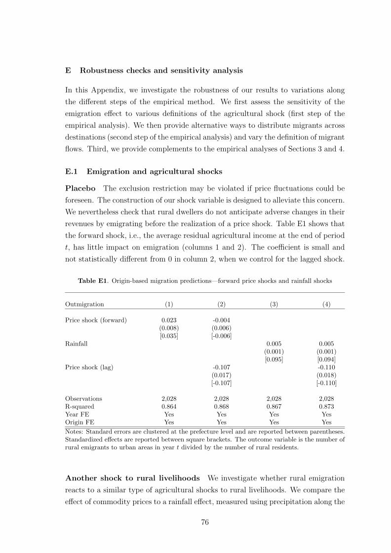
Our findings are robust to numerous sensitivity checks that test the exclusion
restriction, e.g., controlling for agricultural shocks at destination and in neighboring
prefectures, excluding industries that process agricultural goods, omitting local mi-
gration flows, or leveraging forward shocks in a placebo exercise. We also show that
changes in worker composition are unlikely to explain the negative impact on wage
and labor productivity, and that firm entry and exit only amplifies these effects.
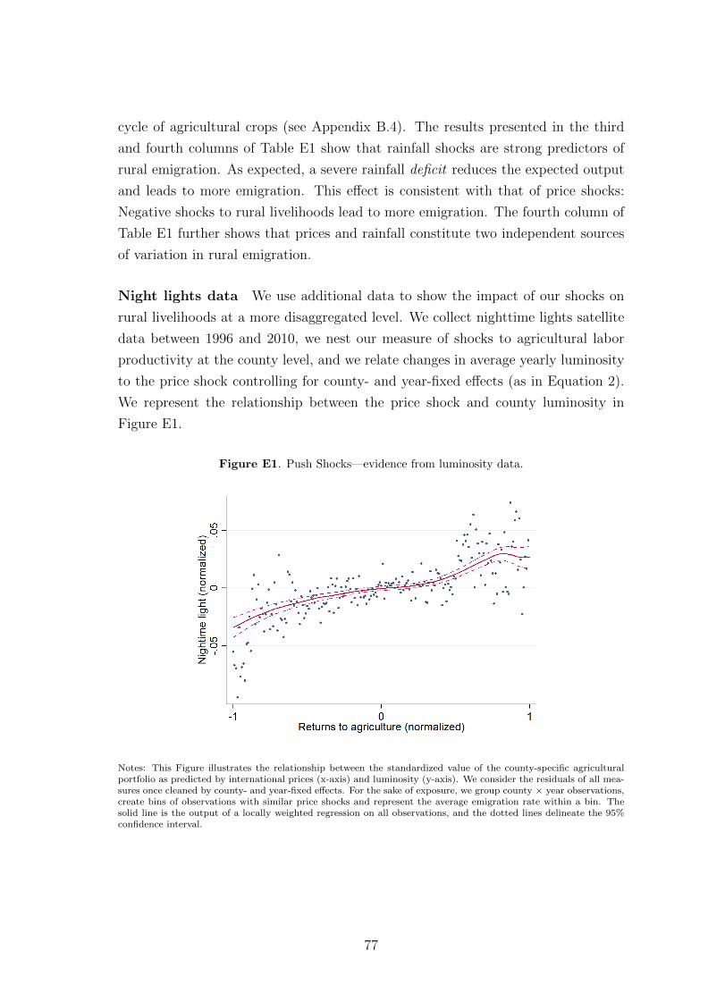
In order to better understand the impact of labor inflows on factor productivity,
we develop a model in which production is characterized by sector-specific elasticities
of substitution between factors and between differentiated final goods, and firm-
specific factor distortions (Hsieh and Klenow, 2009). We estimate the sector-specific
elasticities of substitution between capital and labor following Oberfield and Raval
(2014), and using origin-driven migration shocks as an instrument for relative factor
costs. The quantitative framework suggests that production becomes too labor-
abundant at destination—capital and labor being complements in production—,
and the shift in factor use negatively affects labor productivity. This approach also
allows us to characterize recruiting firms and distinguish them along their ex-ante
factor productivities: Immigrants are primarily recruited by low-productivity firms
within a location, thereby contributing to lower aggregate labor productivity.
Finally, we implement a counterfactual experiment in which we keep constant the
allocation of labor across locations between 2001 and 2006 to quantify the influence
of migration on recent dynamics of the urban economy.2 We show that the continu-
ous migration flows largely contributed to wage moderation in cities, and that their
distributional aspect had consequences on the dynamics of factor productivity (e.g.,
moderating its secular growth, Brandt et al., 2012) and its dispersion across loca-
tions. The systematic migration towards destinations where manufacturing firms
2The Chinese manufacturing sector has grown fast in the past decades, fueled by massivemigration flows from rural to urban areas. The share of agricultural employment in China droppedfrom 70% to 30% between 1980 and 2014, a shift that spanned more than 100 years in mostindustralized countries (Alvarez-Cuadrado and Poschke, 2011).
3
are capital-abundant, productive and paying high wages reduces the dispersion in
relative factor use and factor productivity across locations.
This paper makes significant contributions to two main strands of the literature.
First, this research closely relates to the nascent literature studying how labor supply
shocks impact the structure of production (Lewis, 2011; Peri, 2012; Accetturo et
al., 2012; Olney, 2013; Dustmann and Glitz, 2015; Kerr et al., 2015). Our empirical
analysis borrows from these papers but applies it to a different context: a developing
economy with massive rural-to-urban migration flows and large labor frictions. The
analysis in such context echoes an older literature on migration and unemployment
in cities of developing economies (Todaro, 1969; Harris and Todaro, 1970; Cole and
Sanders, 1985). The theory developed in Harris and Todaro (1970) is based on the
puzzling observation that large migration flows towards cities are observed together
with high unemployment and a large informal sector (Fields, 1975).3 Recent papers
indeed provide evidence of large search and information frictions in accessing formal
jobs (Franklin, 2018; Abebe et al., 2016; Alfonsi et al., 2017). One main contribution
of the research is to document a consequence of these urban labor market frictions,
directly observed from the firm side: the heterogeneous allocation of migrants into
production units.
There is a vibrant literature on productivity gaps across space and sectors (Gollin
et al., 2014; Brandt et al., 2013). In models of labor allocation (Bryan and Morten,
2015; Tombe and Zhu, 2015), mobility frictions are inferred from observed differences
in productivity across locations, and rural-urban migration flows adjust in order to
reduce these differences. A contribution of our analysis is to propose an empirical
counterpart to these analyses. We provide well-identified empirical evidence on the
allocation of labor inflows at the firm level. A counterfactual exercise allows to quan-
tify the role of migration in equalizing productivity across locations. Our findings
suggest that labor market frictions across and within locations are paramount to
explaining firm productivity and its dispersion in developing economics.4
Second, our empirical investigation sheds light on disparities in productivity
and factor allocation across firms of developing economies in general, and China in
particular (Hsieh and Klenow, 2009; Song et al., 2011). We show, in particular,
3One explanation behind this puzzle is the existence of a subsistence income in cities, or labormarket imperfections related to the existence of formal and informal labor markets (Satchi andTemple, 2009; Meghir et al., 2015; Ulyssea, 2018). Another institutional factor which could affectthe absorption of migrants into cities is the existence of minimum wage regulations; the impact ofminimum wages in Chinese cities is discussed in Mayneris et al. (2014).
4Another important source of misallocation in China is the presence of state-owned firms andtransformation of the public sector in the past decades (Hsieh and Song, 2015; Brandt et al., 2016).Our results do not seem to be driven by public-private sector differences.
4
that migrants are recruited by low-productivity firms at destination, which tends
to widen disparities in factor productivity. A large literature has documented the
role of credit market imperfections in generating dispersion in factor returns across
firms, even within the same sector and location (Buera et al., 2011; Midrigan and Xu,
2014; Gopinath et al., 2017). The empirical observation that production becomes
too labor-intensive after a migrant inflow, in spite of production complementarities
between capital and labor, is consistent with large credit market imperfections.
The paper also relates to the large literature on the effects of immigration on labor
markets (Card and DiNardo, 2000; Card, 2001; Borjas, 2003), and more specifically
to studies of internal migration. Among others, Boustan et al. (2010), El Badaoui
et al. (2017), Imbert and Papp (2016) and Kleemans and Magruder (2018) study
the labor market effects of internal migration in the United States in the 1930s, and
in today’s Thailand, India and Indonesia, respectively. In China, the evidence is
mixed: De Sousa and Poncet (2011), Meng and Zhang (2010) and Combes et al.
(2015) respectively find a negative effect, no effect and a positive impact on local
wages. In a more structural approach, Ge and Yang (2014) show that migration
depressed unskilled wages in urban areas by at least 20% throughout the 1990s and
2000s, and our estimates are comparable.
Finally, the research pertains to the literature on structural transformation,
which describes the secular movement of factors from the traditional sector to the
modern sector in developing economies (Lewis, 1954; Herrendorf et al., 2013). The
finding that migration lowers wages and boosts urban employment relates to “labor
push” models, which generally imply that, by releasing labor, agricultural productiv-
ity gains may trigger industrialization (Alvarez-Cuadrado and Poschke, 2011; Gollin
et al., 2002; Bustos et al., 2016). However, we find that migration from rural areas is
triggered by negative shocks to agricultural productivity (as in Groger and Zylber-
berg, 2016; Feng et al., 2017; Minale, 2018, for instance). This suggests that worse
economic conditions at origin lower the opportunity cost of migrating rather than
tightening liquidity constraints on migration (Angelucci, 2015; Bazzi, 2017).5
The remainder of the paper is organized as follows. Section 2 presents data
sources and the estimation strategy. Section 3 describes the reduced-form results on
labor cost and factor use in the average manufacturing firm. Section 4 provides a
quantitative framework to derive implications for factor productivity at destination.
Section 5 briefly concludes.
5In order to identify migration inflows that are exogenous with respect to firms at destination,our paper takes the opposite approach to “labor pull” models, in which rural migrants are attractedby increased labor productivity in manufacturing (see Facchini et al., 2015, using trade shocks).
5
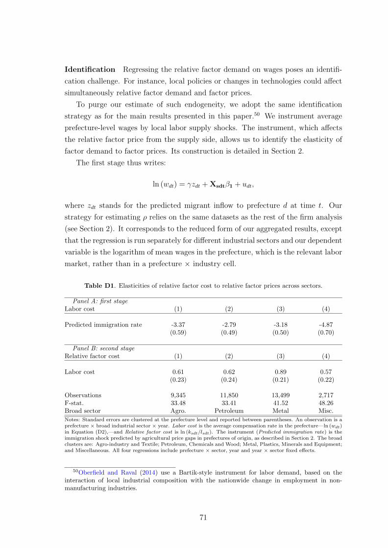
2 Data and empirical strategy
This section describes the data sources and our empirical strategy. We first explain
how we measure migration flows in the data. Next, we construct an instrument for
migration inflows to urban areas based on shocks to agricultural labor productivity
and historical migration patterns. We then present the firm data and describe our
main estimation strategy.
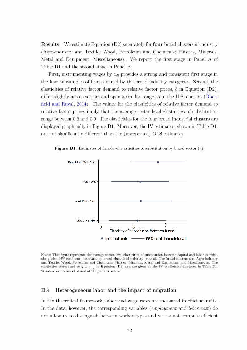
2.1 Migration flows
To construct migration flows, we use the representative 2005 1% Population Survey
(hereafter, “2005 Mini-Census”), collected by the National Bureau of Statistics.6
The sampling frame of the 2005 Mini-Census covers the entire population at current
places of residence, including migrants and anyone who is not registered locally. The
survey collects information on occupation, industry, income, ethnicity, education
level, housing characteristics and, crucially, migration history. First, we observe the
household registration type or hukou (agricultural or non-agricultural) and place of
registration and residence at the prefecture level. Second, migrants are asked the
main reason for leaving their places of registration and which year they left (up to five
years before the date of interview). We combine these two pieces of information to
create a matrix of yearly rural-to-urban migration spells “for labor reasons” between
all Chinese prefectures from 2000 to 2005.7
A raw measure of migration flows would not account for two types of migration
spells: step and return migration. Step migration occurs when migrants transit
through another city before reaching their destination. In such cases, we mistake the
date of departure from the place of registration for the date of arrival at the current
destination. When there is return migration, migrants may leave their place of
registration within the last five years and come back between two census waves. We
then miss the entire migration episode. Fortunately, the 2005 Mini-Census collects
information on the place of residence one and five years before the interview, which
allows us to partly measure return and step migration. We adjust migration flows
allowing for variation in destination- and duration-specific rates of return.8
6These data are widely used in the literature (Combes et al., 2015; Facchini et al., 2015; Mengand Zhang, 2010; Tombe and Zhu, 2015, among others).
7During our period of interest, barriers to mobility come from restrictions due to the registrationsystem (hukou). These restrictions do not impede rural-to-urban migration but limit benefits ofrural migrants’ long-term settlement in urban areas. See Appendix A.1 for more details about howmobility restrictions are applied in practice and the rights of rural migrants in urban China.
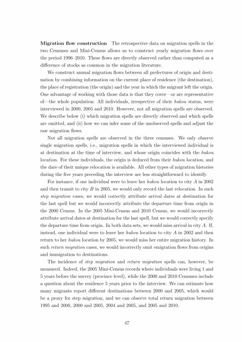
8We show in Appendix A that, while return migration is substantial, step migration is neg-ligible. See Appendix A.2 for more details about the correction for return migration. Resultspresented in the baseline empirical analysis are corrected for return migration but remain robust
6
Let Modt denote the number of workers migrating between origin o (rural areas
of prefecture o) and destination d (urban areas of prefecture d) in a given year
t = 2000, . . . , 2005. The emigration rate, Oot, is obtained by dividing the sum of
migrants who left origin o in year t by the number of working-age residents in o in
2000, which we denote with No:
Oot =
∑dModt
No
.
The probability that a migrant from origin o migrates to destination d at time t,
λodt verifies:
λodt =Modt∑dModt
The immigration rate, mot, is obtained by dividing the sum of migrants who arrived
in destination d in year t by the number of working-age residents (non-migrants) in
d at baseline, in 2000, which we denote with Nd, rescaled by the employment rate
in manufacturing (µ ≈ 14.35%),
mdt =
∑oModt
Nd × µ.
To estimate the causal effect of migrant inflows on urban destinations, we need
variation in immigration that is unrelated to potential destination outcomes. The
next section describes our strategy, based on shocks to rural livelihoods.
2.2 Migration predictions
Our empirical strategy relies on a shift-share instrument (Card, 2001). We inter-
act two sources of exogenous variation to isolate a supply (or push) component in
migrant inflows. First, we use changes in agricultural productivity at origin as ex-
ogenous determinants of migrant outflows from the rural areas of each prefecture.
We construct shocks to labor productivity in agriculture as an interaction between
origin-specific cropping patterns and exogenous price fluctuations. Second, we use
the settlement patterns of earlier migration waves to allocate rural migrants to ur-
ban destinations. This two-step method yields a prediction of migrant inflows to
urban areas that is exogenous to variation in urban factor demand.
Potential agricultural output We first construct potential output for each crop
in each prefecture as the product of harvested area and potential yield. These data
to using non-adjusted flows (see a sensitivity analysis in Appendix E and Appendix Table E2).
7
are provided by the Food and Agriculture Organization (FAO) and the Interna-
tional Institute for Applied Systems Analysis (IIASA).9 The 2000 World Census of
Agriculture offers a geo-coded map of harvested area for each crop, which we use
to construct total harvested area hco for a given crop c and a given prefecture o.
Information on potential yield per hectare, yco, for each crop c and prefecture o
comes from the Global Agro-Ecological Zones (GAEZ) Agricultural Suitability and
Potential Yields dataset. We compute potential agricultural output for each crop in
each prefecture as the product of harvested area and potential yield, qco = hco× yco.By construction, qco is time-invariant and captures cropping patterns at origin. It is
measured at the beginning of the study period, and is thus arguably exogenous to
future migration changes in response to price shocks.10 Figure 1 displays potential
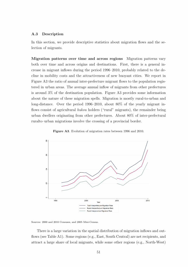
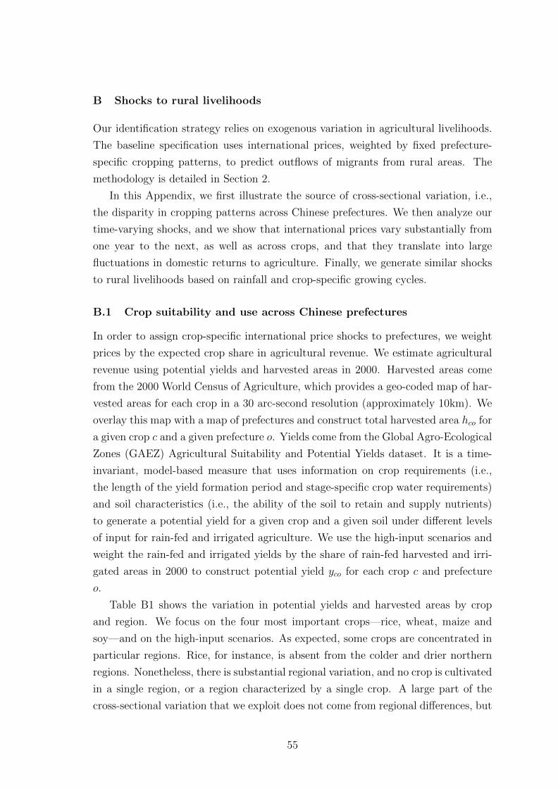
output qco for rice and cotton by prefecture, and illustrates the wide cross-sectional
variation in agricultural portfolios. Appendix B provides summary statistics about
the variation in cropping patterns across prefectures and regions.
Price fluctuations The time-varying component of our push shock is fluctuations
in international commodity prices. We collect monthly commodity prices on inter-
national market places from the World Bank Commodities Price Data (“The Pink
Sheet”).11 We use monthly prices per kg in constant 2010 USD between 1990 and
2010 for 17 commodities.12 These crops account for the lion’s share of agricultural
production over the period of interest: 90% of total agricultural output in 1998
and 80% in 2007. We apply a Hodrick-Prescott filter to the logarithm of nominal
monthly prices and compute the average annual deviation from the long-term trend,
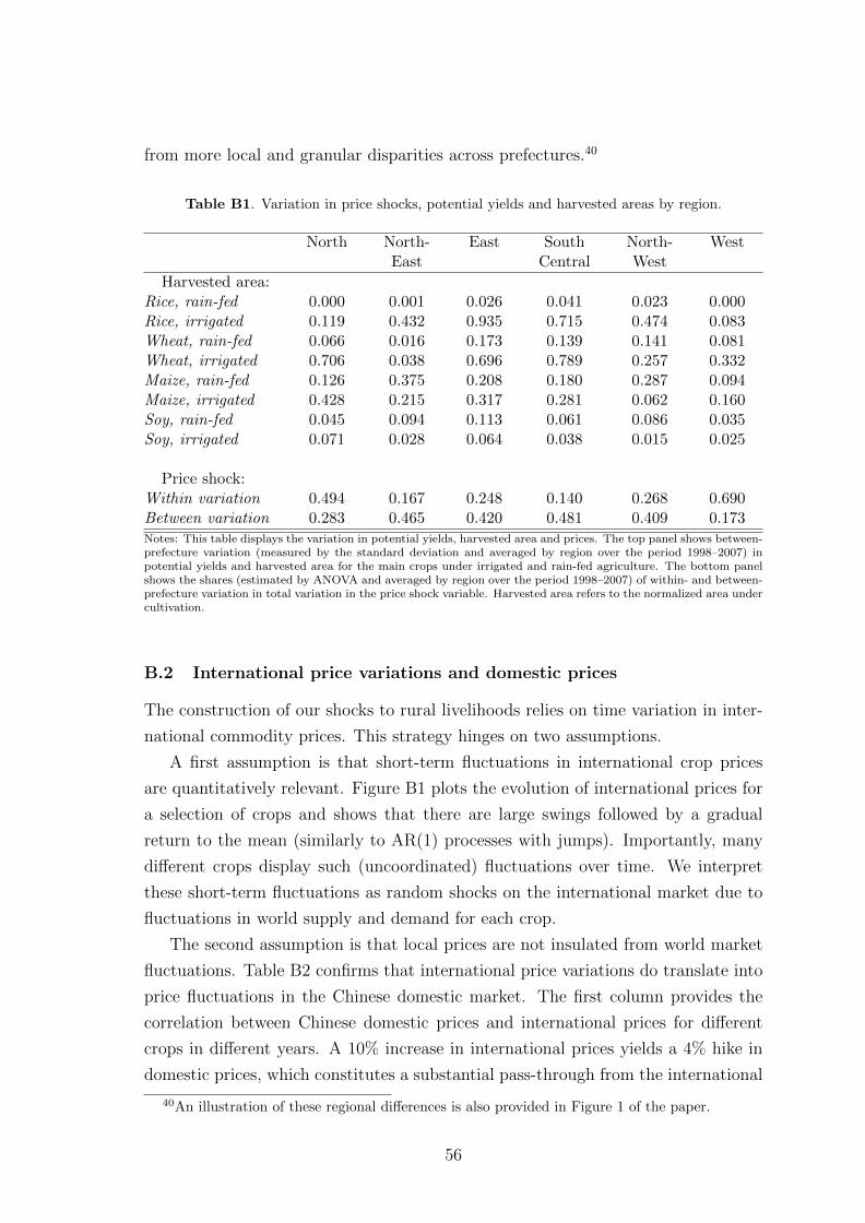
dct. Changes in dct capture short-run fluctuations in international crop prices.13
For these shocks to influence migration decisions, there should be significant
pass-through from international prices to domestic prices faced by rural farmers. In
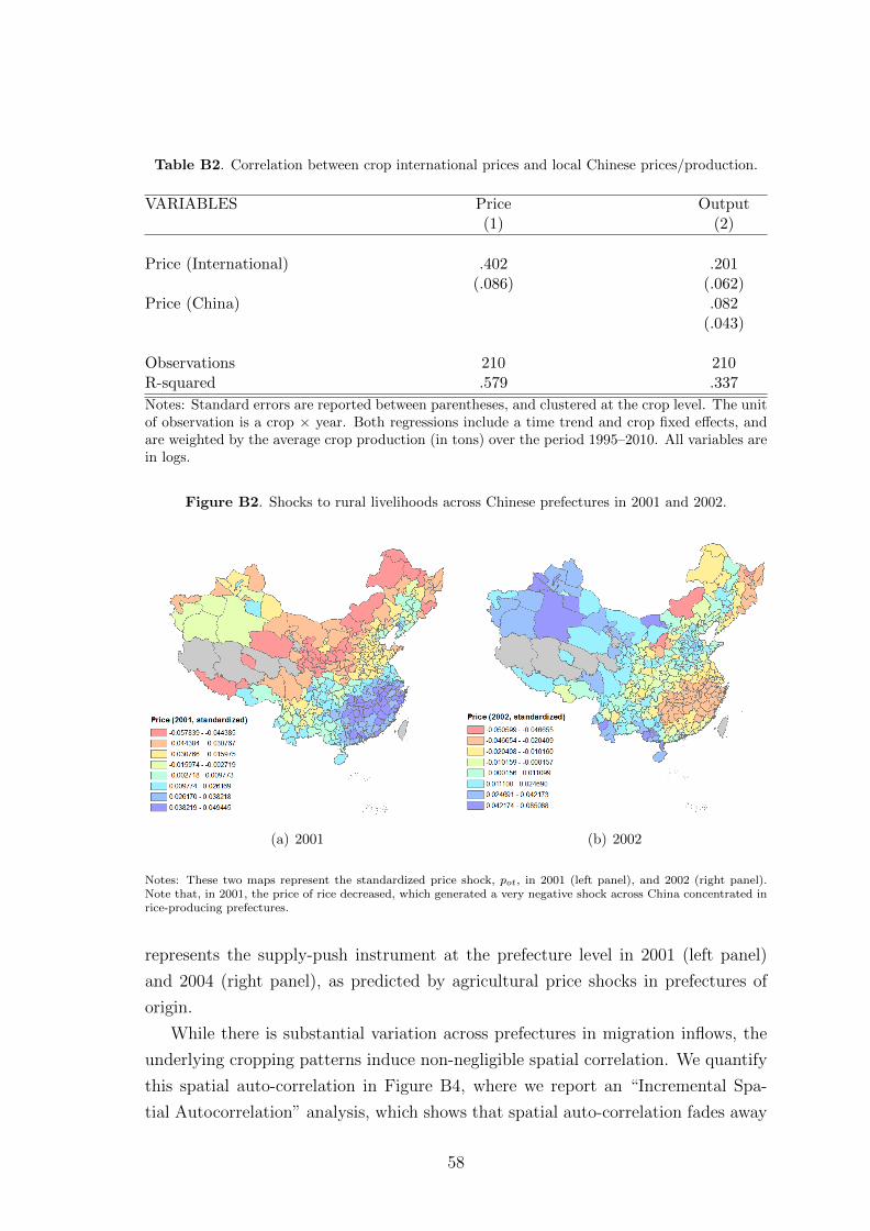
Appendix B, we use producer prices, exports and production as reported by the
FAO between 1990 and 2010 for China and show that fluctuations in international
prices are transmitted to the average Chinese farmer.
9The data are available online from http://www.fao.org/nr/gaez/about-data-portal/en/.10To the extent that price shocks are anticipated, changes in cropping patterns should attenuate
their effect on income and migration, which would bias our first stage coefficients toward zero.11The data are freely available online at http://data.worldbank.org/data-catalog/
rice, sorghum, soybean, sugar beet, sugar cane, sunflower, tea and wheat. We exclude from ouranalysis tobacco, for which China has a dominant position on the international market.
13We apply a Hodrick-Prescott filter with a parameter of 14,400 in order to exclude medium-run fluctuations in prices. We provide in Appendix B descriptive statistics on the magnitude offluctuations across crops. The residual fluctuations in prices behave as an auto-regressive process,but the amplitude of innovation shocks is non-negligible.
Push Shocks We combine the variations in crop prices with cropping patterns to
construct the excess value of crop production in each prefecture o and year t. The
residual agricultural income, pot, is the average of the crop-specific deviations from
long-term trend, {dct}c, weighted by the expected share of agricultural revenue for
crop c in prefecture o:
pot =
(∑c
qcoPcdct
)/
(∑c
qcoPc
)(1)
where Pc denotes the international price for each crop at baseline.
The residual agricultural income exhibits time-varying volatility coming from
world demand and supply, but also large cross-sectional differences due to the wide
variety of harvested crops across China.14 Fluctuations in the measure pot exhibit
part of the persistence already present in international crop prices. A negative
shock does not only affect labor productivity in the same year but also expected
labor productivity, which helps trigger migration outflows.15
Exogenous variation in migrant outflows We now generate an instrument for
migrant flows based on the measure of residual agricultural income and exogenous to
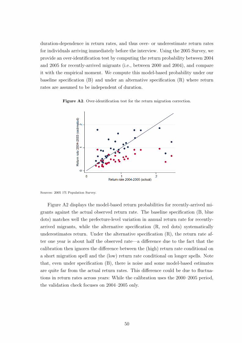
local demand conditions. A migration spell recorded at date t = 2005, for instance,
corresponds to a migrant worker who moved between October 2004 and October
2005. Emigration is likely to be determined not only by prices at the time of harvest,
but also by prices at the time of planting, which determine expected agricultural
revenues, and by prices in previous years due to lags in migration decisions. As a
measure of shock to rural livelihood, sot, we thus use the average residual agricultural
income pot between t− 1 and t− 2.
We regress rural migrant outflows, Oot, on shocks to agricultural income. For-
mally, we estimate the following equation:
Oot = β0 + β1sot + δt + νo + εo,t, (2)
where o indexes the origin and t indexes time t = 2000, . . . , 2005, δt are year fixed
effects, and νo denotes origin fixed effects and captures any time-invariant charac-
teristics of origins, e.g., barriers to mobility.16 We use baseline population (No) as a
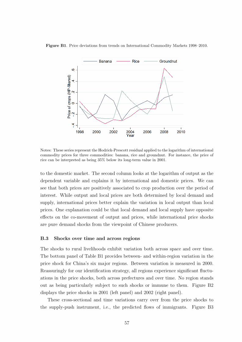
14As an example, Appendix Figure B2 displays the spatial dispersion in pot in 2001, when therice price decreased sharply, and in 2002, after recovery. Appendix Table B1 decomposes thevariation in the measure pot between time-series and cross-sectional variations.
15We show in Appendix B.4 (and Appendix Table E1) that we find similar results when we usefluctuations in agricultural output due to rainfall shocks, which are not serially correlated.
16Incorporating price trends in the analysis does not change the results. We also estimate the
9
weight to generate consistent predictions in the number of emigrants.
We present the estimation of Equation (2) in Panel A of Table 1, including and
excluding short-distance migration spells. Between 2000 and 2005, emigration was
negatively correlated with price fluctuations. A 10% lower return to agriculture,
as measured by the residual agricultural income, is associated with a 0.9 − 1 p.p.
higher migration incidence. Equivalently, a one standard deviation increase in the
shock to rural livelihood decreases migration incidence by about 0.10 standard de-
viations. In theory, fluctuations in agricultural labor productivity may have two
opposite effects on migration (Bazzi, 2017). On the one hand, a negative shock to
agricultural productivity widens the gap between urban and rural labor productiv-
ity and should push rural workers toward urban centers (an opportunity cost effect).
On the other, low agricultural productivity reduces household wealth and its ability
to finance migration to urban centers (a wealth effect). The negative relationship
between agricultural income shocks and migration suggests that migration decisions
are mostly driven by the opportunity cost of migrating.17 Based on these estimates,
we compute the predicted emigration rate Oot from origin o in year t:
Oot = β0 + β1sot + νo,
from which we remove the year fixed effects to avoid correlation between migrant
flows and trends in outcomes at destination.
Exogenous variation in migration inflows We combine the predicted emigra-
tion rate, Oot, and probabilities to migrate from each origin to each destination for
earlier cohorts, λod.18 The predicted immigration rate to destination d in year t is
defined as:
zdt =
∑o 6=d Oot ×No × λod
Nd × µ, (3)
where No is the rural population at origin, Nd is the working-age urban popula-
tion at destination in 2000, rescaled by the employment rate in manufacturing in
China in 2000, µ. To alleviate concerns that migrant inflows are correlated with des-
tination outcomes, we exclude intra-prefecture migrants. This procedure provides
same specification using forward shocks, i.e., the average residual agricultural income at the endof period t, to show that shocks are not anticipated (Appendix E and Appendix Table E1).
17In the Chinese context, workers migrate without their families, low-skill jobs in cities are easyto find, and the fixed cost of migration is relatively low. Chinese households also have high savings,so that the impact of short-term fluctuations in agricultural prices on wealth is small.
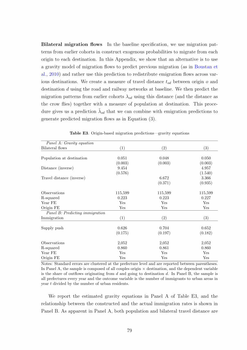
18Alternatively, in Appendix E and Appendix Table E3, we use a gravity model of migrationflows to predict λod as in Boustan et al. (2010). The advantage of using λod is that it includesidiosyncratic variation in migrant networks in addition to geographical factors (Kinnan et al., 2017).
10
supply-driven migrant inflows that are orthogonal to labor demand at destination.
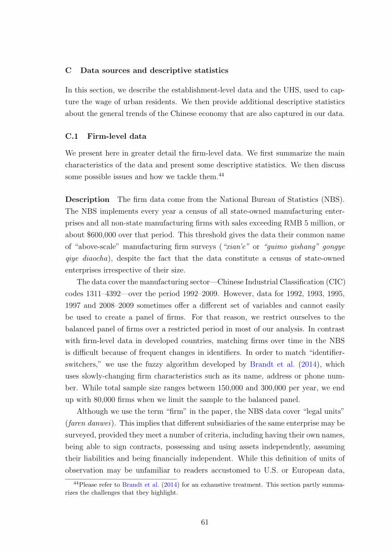
There is spatial auto-correlation due to the geographic determinants of cropping pat-
terns at origin. The shocks however display large cross-sectional and time-varying
fluctuations.19
We regress the actual immigration rate on the predicted, supply-driven immigra-
tion rate and report the results in Panel B of Table 1. The relationship is positive
and significant throughout the sample period: The origin-based variation in the ar-
rival of recent immigrants, zdt, is a strong predictor of observed labor inflows. This
relationship constitutes the first stage of our empirical analysis.
2.3 Description of the firm data
We use firm-level data spanning 2001–2006 from the National Bureau of Statistics
(NBS).20 The NBS implements every year a census of all state-owned manufactur-
ing enterprises and all non-state manufacturing establishments with sales exceeding
RMB 5 million or about $600,000. While small firms are not included in the census,
the sample accounts for 90% of total manufacturing output. Firms can be matched
across years, and a large part of the analysis will be performed on the balanced
panel (about 80,000 firms). The NBS census collects information on location, in-
dustry, ownership type, exporting activity, number of employees and a wide range
of accounting variables (sales, inputs, value added, wage bill, fixed assets, financial
assets, etc.). We divide total compensation (to which we add housing and pen-
sion benefits) by employment to compute the compensation rate, and construct real
capital as in Brandt et al. (2014).
There are three potential issues with the NBS census. First, matching firms
over time is difficult because of frequent changes in identifiers. We extend the fuzzy
algorithm (using name, address, phone number, etc.) developed by Brandt et al.
(2014) to the period 1992–2009 to detect “identifier-switchers.” Second, although
we use the term “firm” in this paper, the NBS data cover “legal units” (faren dan-
wei), which roughly correspond to the definition of “establishments” in the United
States.21 Third, the RMB 5 million threshold that defines whether a non-publicly
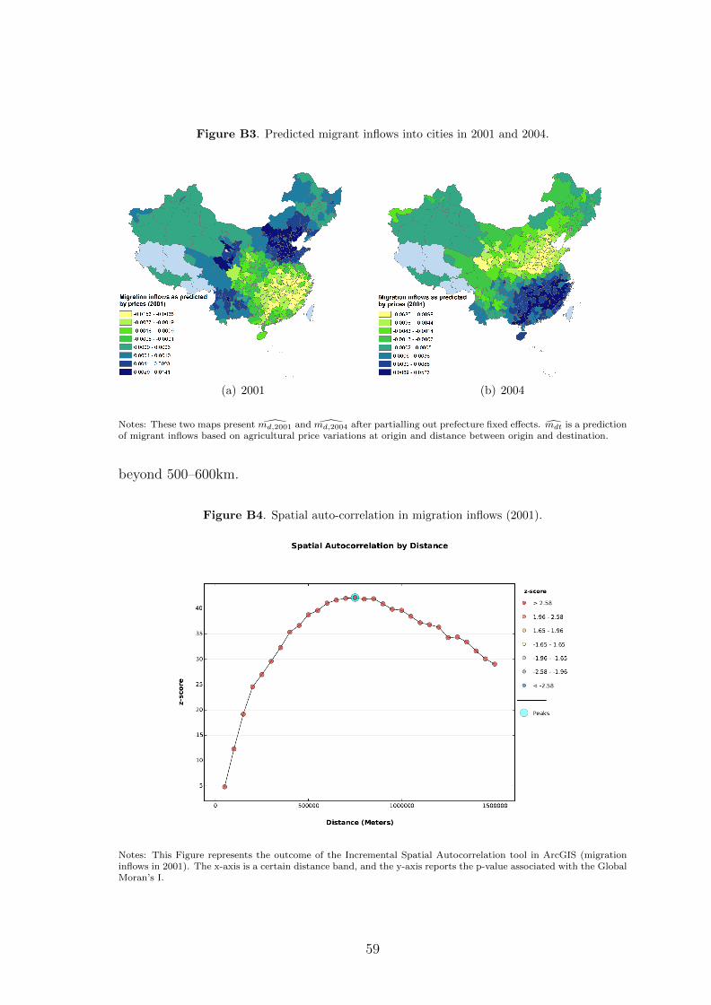
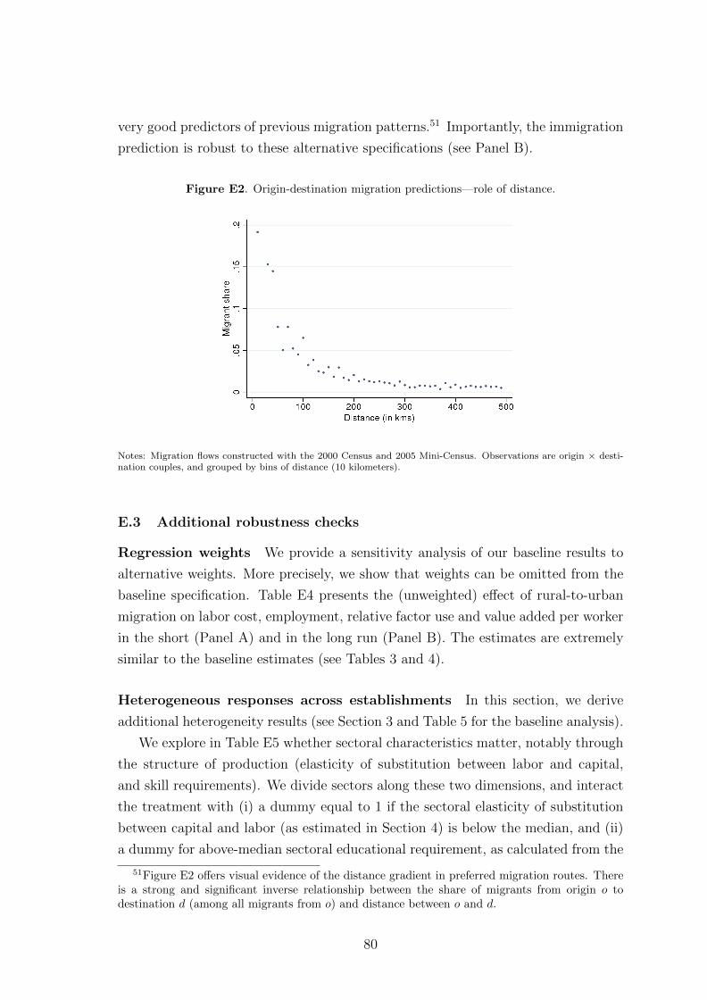
19We provide in Appendix B an illustration of this spatial auto-correlation. Appendix Figure B3,shows the geographical distribution of zdt in 2001 (left panel) and 2004 (right panel), after takingout prefecture fixed effects.
20The following discussion partly borrows from Brandt et al. (2014), and a detailed descriptionof construction choices is provided in Appendix C.
21Different subsidiaries of the same enterprise may indeed be surveyed, provided they meet anumber of criteria, including having their own names, being able to sign contracts, possessingand using assets independently, assuming their liabilities and being financially independent (seeAppendix C). In 1998, 88.9% of firms reported a single production plant. In 2007, the share ofsingle-plant firms increased to 96.6% (Brandt et al., 2014).
11
owned firm belongs to the NBS census is not sharply implemented. Hence, some
private firms may enter the database a few years after having reached the sales cut-
off or continue to participate in the survey even if their annual sales fall below the
threshold. We cannot measure delayed entry into the sample, but delayed exit of
firms below the threshold is negligible, as Figure 2 shows.
Our main outcomes include compensation per worker, employment, capital-to-
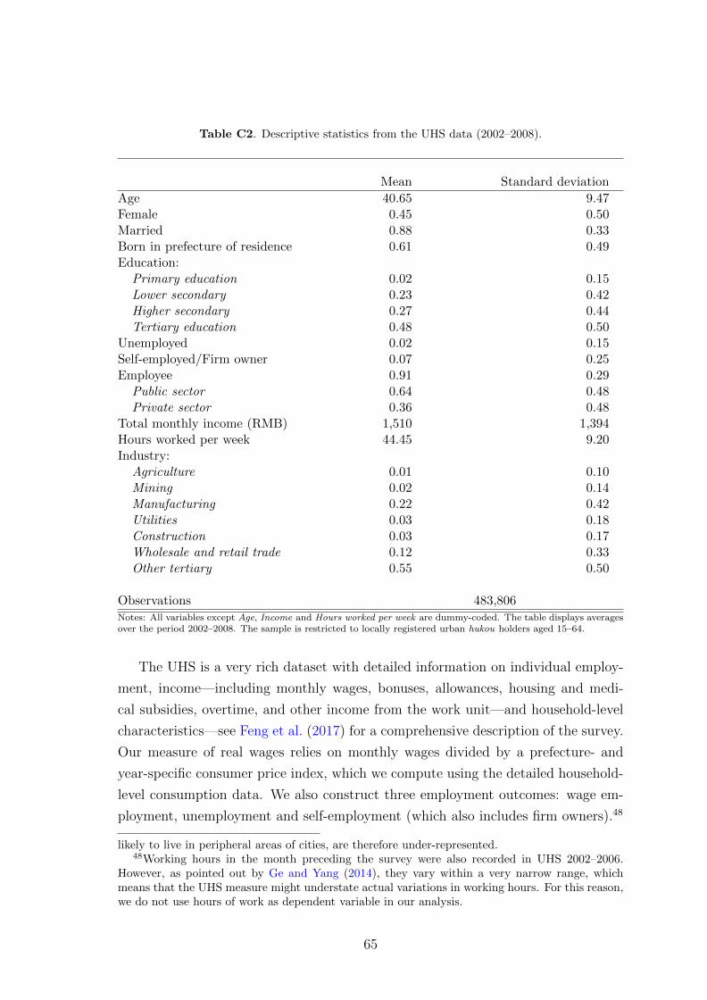
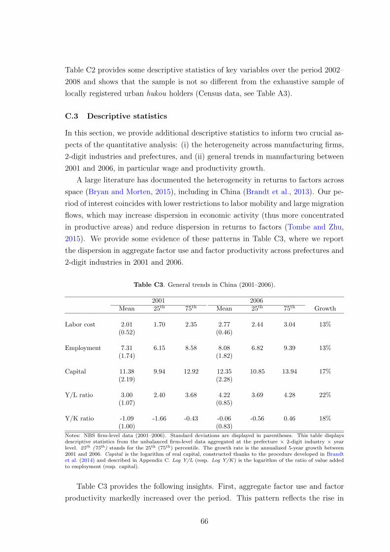
labor ratio and value added per worker. Table 2 provides descriptive statistics of
our key outcomes at the firm-level in 2001. There is substantial heterogeneity in
firm outcomes, both within and across locations.22
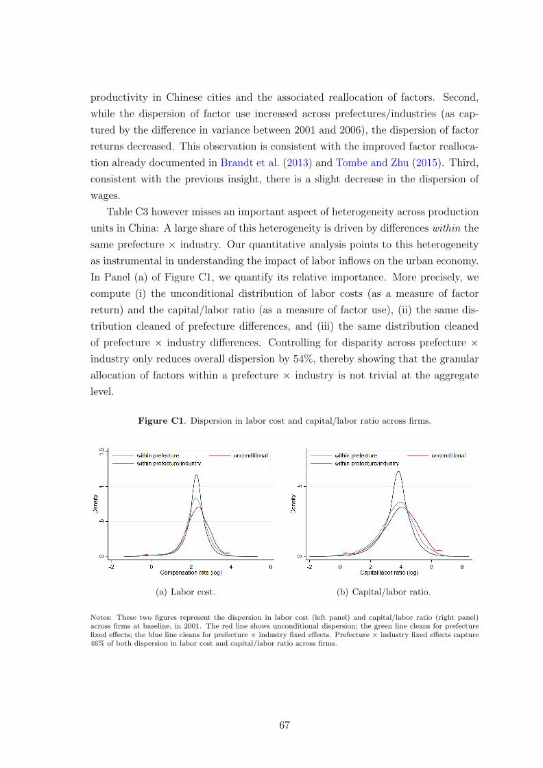
2.4 Empirical strategy
We use two main specifications, depending on whether we estimate the short-term
effect on the average firm, or longer-run effects using cumulative migration between
2001 and 2006.
Short-run effects We first exploit yearly time-variations in the full panel. The
unit of observation is a firm i in year t and prefecture d. We estimate an IV speci-
fication and regress the dependent variable yidt on the recent immigration rate mdt:
yidt = α + βmdt + ηi + νt + εidt (4)
where ηi and νt are firm and time fixed effects, and mdt is instrumented by the
supply-driven predicted immigration rate, zdt. Standard errors are clustered at the
level of the prefecture.
Longer-run effects To estimate the longer-run impact of migration on urban
production, we estimate the effect of cumulative migration shocks between 2001 and
2006 on changes in firm outcomes over the period. Letting md (resp. zd) denote the
average yearly immigration rate (resp. the average yearly supply-driven predicted
immigration rate) in destination d between 2001 and 2006, and ∆yid denote the
difference in outcomes between 2001 and 2006, we estimate:
∆yijd = α + βmd + νj + εijd (5)
where md is instrumented by zd, and νj are sector fixed effects. Standard errors are
clustered at the level of the prefecture of destination.
22We leave the analysis of general trends in China and differences across establishments of thesample to Appendix C, and Appendix Tables C1 and C3 in particular. This analysis shows thatmanufacturing growth is very unequally shared across prefectures.
12
In order to identify heterogeneous effects, we estimate:
where Xi is a time-invariant characteristic of firm i. The time-invariant characteris-
tics, Xi, will be dummy variables capturing the relative factor-intensity and factor
productivity at baseline within a sector × prefecture. As in the previous specifica-
tion, νj denotes sector fixed effects, and µj are characteristic × sector fixed effects.
md is instrumented by zd, and its interaction md ×Xi is instrumented by zd ×Xi.
3 Migration, labor cost and factor demand
In this section, we quantify the effect of the labor supply shift on labor cost and
factor demand, both on impact and in the longer-run. We then analyze heteroge-
neous responses depending on baseline firm characteristics, most notably a measure
of relative labor productivity at destination. We complete this section with a com-
prehensive sensitivity analysis exploring variations along the baseline specification,
a placebo test using future shocks to agricultural livelihoods, and a measure of labor
cost cleaned of compositional adjustments.
3.1 Average effect on labor cost and factor demand
Short-run effects An important and debated consequence of migration is its
short-run effect on wages at destination. We estimate specification (4) on the sub-
sample of firms present all years between 2001 and 2006 and use total compensation
per employee (including fringe benefits) as a proxy for labor cost. The first column
of Table 3 displays the OLS estimate (Panel A) and the IV estimate (Panel B). An
inflow of rural migrants is negatively associated with labor cost at destination. Since
migrants should be attracted to cities that offer numerous employment opportunities
and high wages, the OLS estimate should be biased upwards.23 We indeed find a
more negative price elasticity of labor demand in the IV specification, in which
the immigration rate is instrumented by the labor supply shock. A one percentage
point increase in the immigration rate induces a 0.53% decrease in compensation
per employee. This large response of wages to immigration is comparable to other
23The association between fluctuations in factor cost and factor use and variation in rural-to-urban migration may result from “pull” factors and “push” shocks. In the IV specification, onlypush factors contribute to the correlation between migration and the urban economy at destination.In general, we find differences between OLS estimates and IV estimates to be small, except for theprice of labor. These findings are not related to an issue of weak instruments; our instrument is astrong predictor of the immigration rate at destination in all baseline specifications.
13
studies of internal migration in developing economies (Kleemans and Magruder,
2018). Internal migrants in China could be more easily substitutable with “natives”
than international migrants in developed countries (see, e.g., Borjas, 2003, for the
United States).24
Following a positive labor supply shock, manufacturing firms should expand and
become more labor-abundant. Our estimates of the impact of migration on factor
demand are presented in columns 2 and 3 of Table 3. An additional percentage point
in the immigration rate increases employment in the average manufacturing firm by
0.36%. Since we normalize the migration rate by the population working in the
manufacturing sector, one would expect the coefficient to be 1 if all newly-arrived
immigrants were to be absorbed by the manufacturing sector without altering the
share of the balanced sample in that sector. Some migrant workers may be hired by
smaller manufacturing firms or work in other sectors (e.g., construction); some of
them may also transit through unemployment or self-employment (Giulietti et al.,
2012; Zhang and Zhao, 2015).
The labor supply shift affects the relative factor use at destination. As shown
in column 3 of Table 3, the capital-to-labor ratio decreases by 0.26% following a
one percentage point increase in the migration rate, which suggests that capital
positively adjusts to the increase in employment but moderately so. There are two
possible reasons behind this finding. Firms that expand may belong to sectors with
relatively high substitutability between capital and labor, in which case a moderate
adjustment of capital could be an optimal response. There may also be credit
constraints and adjustment costs that prevent firms from reaching their optimal use
of production factors in the short run. We shed light on these two interpretations
when investigating treatment heterogeneity and longer-run effects.
The average product of labor appears to fall sharply in response to migrant
inflows. An additional percentage point in the immigration rate decreases value
added per worker by 0.50% (column 4 of Table 3). With employment increasing
(only) by 0.36%, the labor supply shock thus negatively affects value added at the
firm level. Firm expansion may come at a short-run cost; for instance, new hires
may need to be trained and production lines to be adjusted before the expansion
of production factors translates into higher output. We now provide an estimation
of the impact of migration on urban firms in the medium run, when firms can be
24Our findings are in line with recent studies arguing that rural-to-urban migration has markedlytempered wage growth in urban China (De Sousa and Poncet, 2011; Ge and Yang, 2014). The highprice elasticity of labor demand may also illustrate that labor markets in developing countries arerelatively less regulated. For instance, minimum wage regulations in China only came into forcetowards the end of our observation period (Mayneris et al., 2014).
14
expected to have overcome some of these short-run adjustments.
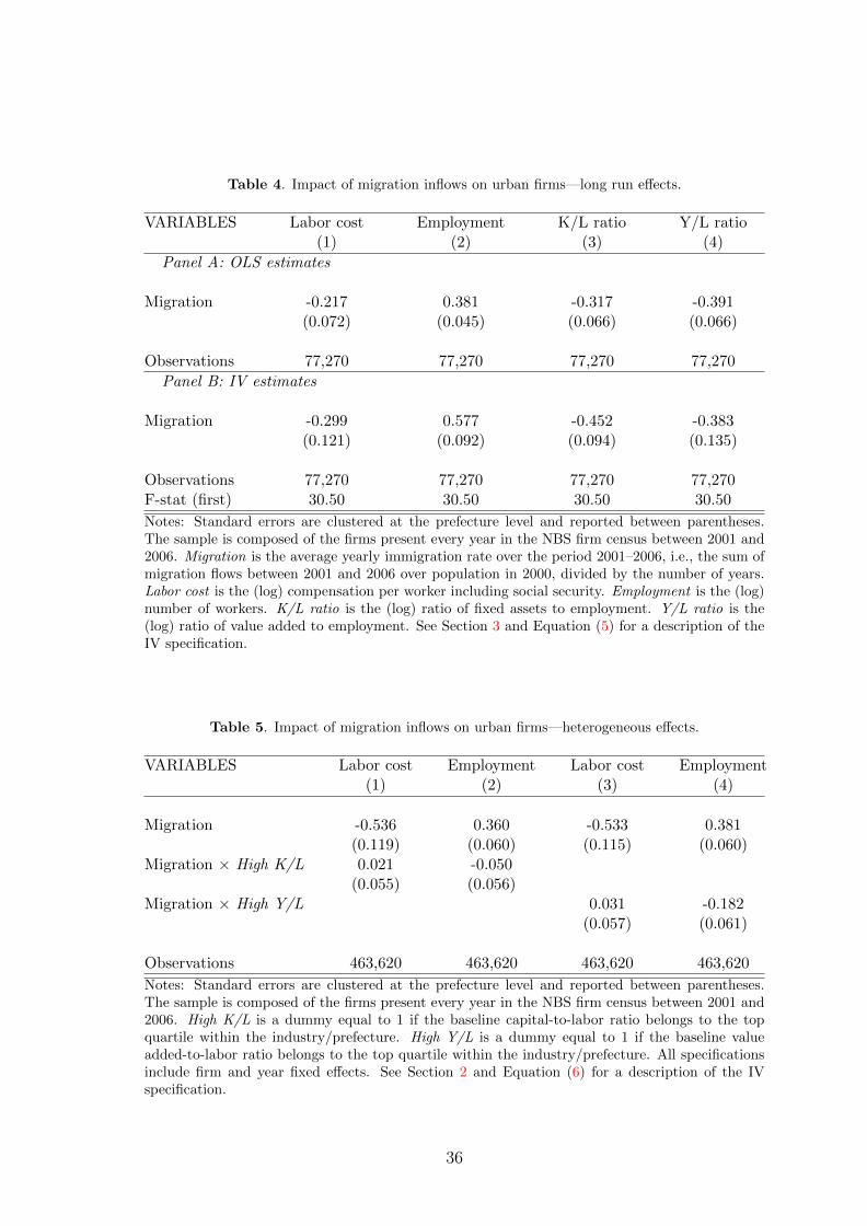
Longer-run effects The effect of migrant inflows on impact may sharply differ
from the longer-run effect. Labor markets at destination may adjust through worker
mobility across prefectures, e.g., prefectures that experienced a wage decrease due
to a sudden migrant inflow may receive fewer migrants in subsequent years (Monras,
2018). Within a destination, local labor supply may also respond to the arrival of
low-skill workers (Llull, 2018). Moreover, capital and investment could adjust over
time, and production lines could be re-optimized to accommodate for the arrival of
new workers. We investigate these long-run effects using specification (5), and we
report the impact of the labor supply shift on factor cost, factor demand and value
added per worker in Table 4.
The price elasticity of labor demand in the longer run, −0.30, is lower than the
short-run estimate. This wage adjustment occurs in spite of a higher absorption of
migrants within manufacturing firms: An additional percentage point in the immi-
gration rate between 2001 and 2006 increases employment by 0.58%. The impact
of migrant inflows on labor cost and employment strongly affects relative factor
demand: Firms located in prefectures that receive more migration remain labor-
abundant even in the longer run; capital adjustments remain marginal. Finally, the
effect of migration on value added per worker is less negative in the longer run and
induces a positive impact of migration on output at destination. With employment
increasing by 0.58%, a labor supply shock of one percentage point in the immigration
rate increases value added by about 20%.
Overall, the (few) discrepancies between the short- and longer-run impacts of im-
migration are consistent with (i) slow labor market adjustments, (ii) either low levels
of complementarity between capital and labor or non-negligible frictions in access
to capital, and (iii) a disruption of production on impact, explaining why the de-
crease in average labor productivity at the firm-level is partly tempered in the longer
run. While our study cannot provide any direct insight about the consequences of
large rural-to-urban migration over a long period, the behavior of manufacturing
firms in China is consistent with Lewis’s (2011) findings for the 1980s and 1990s
in the United States. Firms may choose not to mechanize due to the availability
of cheap labor. They shift investment and technology adoption decisions towards
a more labor-intensive mode of production and this choice locks them over longer
horizons. Such a mechanism would require (already) labor-abundant manufacturing
firms to hire the marginal low-skill worker. We now provide some evidence on the
heterogeneous absorption of migrants in the urban economy.
15
3.2 Heterogeneity in factor demand
We study the heterogeneous response in factor demand by interacting migrant in-
flows with fixed firm characteristics (see Equation 6). We limit our analysis to two
characteristics related to labor needs and leave the analysis along additional dimen-
sions to Appendix E and Appendix Table E5.25 We label as capital-abundant all
firms with a capital-to-labor ratio at baseline in the top quartile within their sec-
tor and prefecture. We label as labor-productive all firms with a value added per
worker at baseline in the top quartile within their sector and prefecture. Under
the assumption that firms in the same sector and prefecture use similar technolo-
gies, a high capital-to-labor ratio indicates a shortage of labor and we should expect
capital-abundant firms to recruit aggressively. Along the same lines, newly arrived
immigrants should be hired by the most productive firms.
Table 5 presents the IV estimates for labor cost and labor demand.26 In columns 1
and 3, we test for the existence of heterogeneous effects of migrant inflows on labor
cost, which could occur if firms with different relative factor use or productivity
recruited in segmented labor markets. The reduction in labor cost is found to be
remarkably homogeneous across firms; more or less capital-abundant or productive
firms appear to face similar labor market conditions. We do not find that capital-
abundant firms recruit more than the average firm (column 2). However, firms
with higher average labor productivity are less likely to expand in response to the
migration shock: A one percentage point increase in the migration rate increases
employment in firms with low value added per worker by 0.38% as against 0.20% in
productive firms.
These findings are puzzling. Migrant workers are not recruited by more “capital-
rich” firms in the same sector and location, and they are predominantly hired by
seemingly unproductive firms. This observation sharply contrasts with empirical
regularities of firm growth in developed economies: Employment growth at the
firm level usually correlates with indicators of productivity; employment flows are
typically directed towards productive firms (see Davis and Haltiwanger, 1998, for
evidence in the U.S. manufacturing sector). The allocation properties of large inflows
of rural migrants appear to differ from the adjustments induced by labor demand
shocks. This finding is however consistent with Lewis (2011), who finds that some
firms respond to migrant inflows by adopting a more labor-intensive organization of
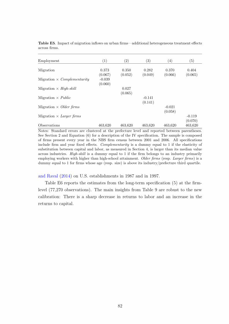
25Appendix Table E5 investigates heterogeneous treatment effects along complementarity be-tween capital and labor, whether an industry predominantly hires high-skill workers, and firmownership, age and size. We do not find strong evidence of heterogeneity along these variables.
26We do not report the estimates for the adjustment of capital-to-labor ratio or value added, asa more systematic heterogeneity analysis will be provided in the next section.
16
production.
One issue with the present analysis is that it does not account properly for
complementarity between factors and uses a crude measure of labor productivity. In
order to better characterize recruiting firms and the impact of recruitment on factor
productivity, we develop in Section 4 a production function estimation allowing
for sector-specific complementarity between factors and residual differences between
firms of the same sector. Before developing this more structural approach, we discuss
the robustness of our baseline reduced-form approach.
3.3 Sensitivity analysis and compositional effects at destination
Sensitivity analysis An important threat to the identification strategy is that
agricultural prices affect the urban sector through other channels than the arrival of
immigrants in cities, notably through markets for goods. Changes in the supply of
agricultural output may affect specific sectors where agricultural output is used as
intermediate input, and the geographical distribution of vulnerable industries may
correlate with migration patterns. Omitted spatial variation in the distribution of
manufacturing firms may also correlate with migration flows. Moreover, cities and
their surroundings may be integrated through final goods markets, so that changes in
agricultural income in rural hinterlands affects demand for manufactured products
in cities (Bustos et al., 2016; Santangelo, 2016).
To alleviate these concerns, we carry out seven robustness checks, which are
presented in Table 6. In Panel A, we report the baseline specification in which
we control for the residual agricultural income shock in the receiving prefecture.
In Panel B, we control for this shock in neighboring prefectures, weighting by the
inverse of travel time computed using the existing transportation network. To fur-
ther alleviate concerns about spatial autocorrelation in agricultural revenue shocks,
we exclude all migrant flows that occur within a 300-km radius of the prefecture’s
centroid when constructing the immigration rate and the instrument (Panel C). In
Panel D, we exclude industries in which agricultural products are used as intermedi-
ate inputs (food processing and beverage manufacturing industries). In Panel E, we
add sector × year fixed effects to control for sector-specific fluctuations. In Panel F,
we control for a measure of market access—the sum of population in all rural pre-
fectures weighted by the inverse of the distance to the prefecture where the firm is
located—fully interacted with year dummies. In all these instances, the estimates
are comparable to the baseline estimates
Finally, we perform a placebo test in which we correlate firm outcomes with
future immigration rate, instrumented by the forward supply push. As Panel G of
17
Table 6 shows, the placebo estimates are all insignificant and much smaller than our
main estimates. The sensitivity analysis supports our main interpretation, i.e., that
shocks to agricultural productivity affect manufacturing firms through the arrival of
new immigrants—as potential workers—into cities.
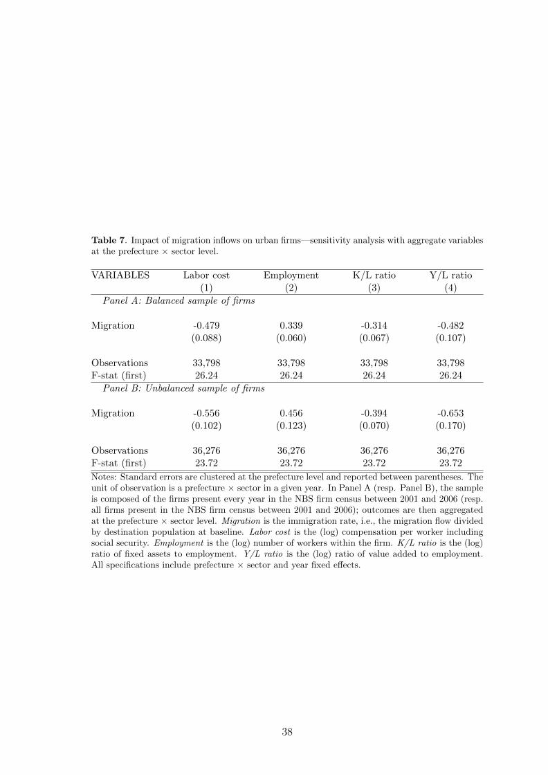
Aggregation and sample choice The baseline specification (4) is estimated at
the firm-level. An alternative empirical specification would be to aggregate quan-
tities at the sector × prefecture level, which could limit the influence of outliers.
In Panel A of Table 7, we use the sample of firms present every year in the NBS
firm census between 2001 and 2006, aggregate outcomes within a cell (prefecture ×sector), estimate a specification similar to Equation (4) where i is a cell instead of
an individual firm, and condition the analysis on cell and year fixed effects. The
IV estimates are found to be robust to this alternative specification, and standard
errors are slightly lower than in the baseline specification.
Our baseline analysis focuses on the balanced sample of firms. However, as
shown in Appendix Table C1 and discussed in Appendix C, the balanced sample
only represents about a third of all firm × year observations. In order to account for
the possible effect of entry into and exit from the NBS census of above-scale firms,
we replicate the previous exercise on the sample of all firm × year observations
between 2001 and 2006 (Panel B of Table 7). The estimated wage response to a one
percentage point increase in the migration rate is −0.56%, very close to the estimate
on the balanced sample (−0.48%). The effects on employment, capital-to-labor ratio
and value added per worker are all larger in magnitude. Including firms that enter
our sample over time and aggregating at the sector × prefecture level strengthens
the finding that production becomes more labor-intensive with migration, and labor
productivity declines.
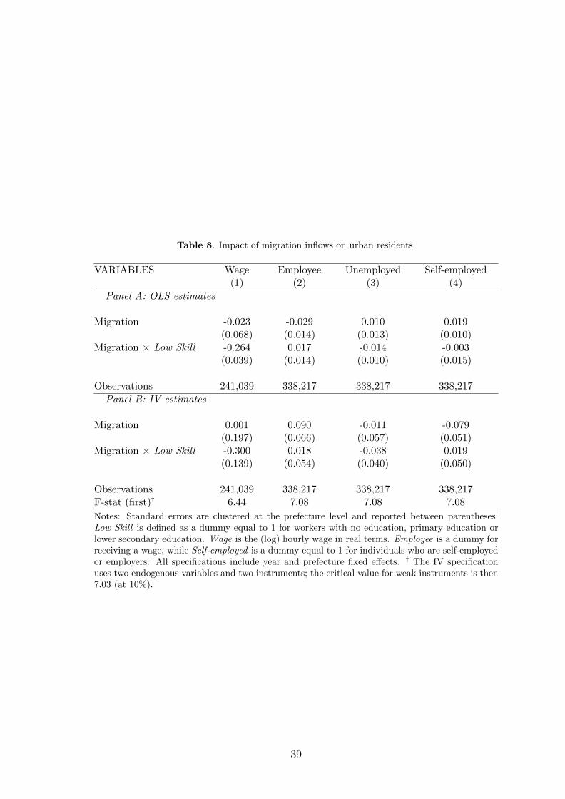
Worker heterogeneity and compositional effects at destination We have
interpreted so far the decrease in labor cost as a decline in the equilibrium wage.
However, compensation per worker may fall due to changes in the composition of
the workforce, as less skilled workers enter the manufacturing sector and potentially
displace skilled resident workers (Card, 2001; Monras, 2015). The NBS data do not
provide yearly information on the skill composition of the workforce or their migrant
status. To clean the price elasticity of labor demand from compositional effects, we
exploit yearly cross-sections of the Urban Household Survey (2002–2006)—a repre-
sentative survey of urban “natives” (see description in Appendix C.2).
The empirical analysis is based on estimating changes in the wage of urban
18
residents triggered by changes in migrant inflows.27 The labor market outcome, yjdt,
of individual j surveyed in prefecture d and year t is regressed on the immigration
rate mdt and its interaction with a dummy Ljdt, equal to 1 if individual j has
secondary education or below.28 More formally, we estimate:
where ηd and θd are destination fixed effects, νt and µt are year fixed effects, sdt are
destination × year fixed effects, and Xjdt is a vector of individual characteristics,
including marital status, gender, education level and age. We estimate Equation (7)
by OLS and in an IV specification where we instrument the immigration rate mdt
and the interaction mdt × Ljdt by the supply shock zdt and its interaction with the
low-skill dummy, zdt × Ljdt.Table 8 presents the results. Column 1 reports the OLS and IV estimates of
β0 and β1, when the dependent variable is a measure of hourly wages adjusted by
the provincial Consumer Price Index. We find no effect of migration on high-skilled
wages (workers with tertiary education), but the wage of less skilled workers falls
by 0.30% when the migration rate increases by one percentage point. In columns
2 to 4 of Table 8, we analyze the possible displacement of urban residents. Rural-
to-urban migration has no significant effect on the allocation of urban residents
between wage employment, unemployment and self-employment, which implies that
the urban residents mostly adjust to an immigration shock by accepting lower wages.
The decrease in wages of low-skill residents accounts for about 60% of the labor
cost response estimated using firm-level data (see Table 3). The discrepancy between
the effect on labor cost and the impact on the wage of residents may be due to various
reasons. The labor markets of residents and migrants may be partly segmented, and
not many residents may be employed in the manufacturing firms of our main sample.
Incumbent worker wages may be more rigid than hiring wages. Finally, migrants
may be less productive than residents, and the recruitment of lower-productivity
workers could account for part of the decline in average labor cost. We provide a
higher bound for this compositional effect in Appendix D.4; the compositional effect
27A recent study uses the Urban Household Survey in 2007 to evaluate the wage effect of migrantinflows across Chinese prefectures and finds a positive effect (Combes et al., 2015). The presentexercise however differs from their analysis along several dimensions. We exploit the quasi-panelstructure of the data and fluctuations over time in the arrival of rural workers; our analysis thusestimates a short-run impact. Moreover, we use a time-varying instrument isolating variation inlabor supply.
28Unskilled urban residents (58% of the sample) are most likely the ones competing for jobswith migrant workers, and hence their response to migration inflows should be different from therest (Card, 2001; Borjas, 2003).
19
can, at most, explain a decrease in the labor cost of −0.08% when the migration
rate increases by one percentage point. Overall, the analysis of worker data confirms
that rural migrant inflows have a strong negative effect on the equilibrium wage in
cities, but limited displacement effects.
4 Migration and factor productivity
This section develops a quantitative framework, in which there are sector-specific
complementarities between capital and labor (Oberfield and Raval, 2014), and in-
dividual firms are characterized by residual factor market distortions (Hsieh and
Klenow, 2009). We use the quantitative model to interpret the impact of labor in-
flows on factor productivity at the prefecture level and to discipline the analysis of
heterogeneity across firms. The last subsection provides a counterfactual analysis
that quantifies the contribution of rural-to-urban migration to the recent wage and
productivity growth (and dispersion) in the Chinese economy.
4.1 Quantitative framework
We first describe a static model of firm production based on Oberfield and Raval
(2014) with two factors, sector-specific complementarity between capital and labor,
monopolistic competition within sectors, and firm-specific wedges in factor prices.
Theoretical framework The economy is composed of D prefectures. In each
prefecture d, the economy is divided into sectors within which there is monopolistic
competition between a large number of heterogeneous firms. The final good is pro-
duced from the combination of sectoral outputs, and each sectoral output is itself a
CES aggregate of firm-specific differentiated goods. Firms face iso-elastic demand
with σ denoting the elasticity of substitution between the different varieties of the
sectoral good. In what follows, we drop prefecture indices for the sake of exposure.
Total sectoral output in a product market (sector × prefecture) is given by the
following CES production function:
y =
[∑i
xiyσ−1σ
i
] σσ−1
, (8)
where xi captures consumer preferences for variety i. Each firm i thus faces the
following demand for the product variety i:
yi = (pi/p)−σxσi y (9)
20
where pi is the unit price for variety i, and p is the aggregate price at the product
market level. We assume that a firm i produces yi according to a CES production
function:
yi = Ai [αkρi + (1− α)lρi ]
1ρ , (10)
where α, governing the capital share, and ρ, governing the elasticity of substitution
between capital and labor, are assumed constant over time and within sector.
As in Hsieh and Klenow (2009), we rationalize differences in factor use across
firms by assuming that individual firms face different firm-specific wedges in factor
prices. Let τ li denote the labor wedge and τ ki denote the capital wedge, respectively
impacting the marginal cost of labor and capital. Firm i maximizes the following
program, taking as given factor prices and the aggregate demand and price at the
product market level,
maxpi,yi,li,ki
{piyi − (1 + τ li )wli − (1 + τ ki )rki
}(11)
subject to the production function (8) and demand for its specific variety (9).
Estimation The following fundamentals of the model need to be estimated: the
degree of substitution between capital and labor (ρ), the capital share (α), the
elasticity of substitution between product varieties (σ)—all at the sector level—,
and firm-specific distortions (τ ki , τli ).
The identification of the model derives from estimating the sector-specific elas-
ticity of substitution between factors. Indeed, conditional on knowing the parameter
ρ at the sector level, α and σ can be imputed from factor shares and the ratio of
profits to revenues. In order to identify ρ, we proceed as Oberfield and Raval (2014):
We rely on the relationship between relative factor demand and factor cost, and we
exploit a labor supply shock to shift the labor cost.29
Optimal factor demand at the firm level verifies:
ln
(rkiwli
)=
1
1− ρln
(α
1− α
)+
ρ
1− ρln(wr
)+
1
1− ρln
(1 + τ li1 + τ ki
),
in which one can separately identify three terms: (i) a sector fixed-effect, (ii) the rel-
ative factor prices at destination weighted by the elasticity of substitution, and (iii)
a measure of firm-specific relative distortions in access to factor markets. Identifying
the elasticity of substitution from this relationship is challenging because omitted
29The derivation of optimal factor demand is made explicit in Appendix D. This Appendix alsodescribes the full identification strategy.
21
variation (e.g., an increase in labor productivity) may influence both relative factor
prices and relative factor use.
We identify the sectoral elasticity of substitution ρ by exploiting exogenous vari-
ation in the relative factor cost induced by our labor supply shock. The arrival of
migrants shifts the relative price of labor downward, an effect that is orthogonal to
omitted variation related to labor demand. We assume, as in Oberfield and Raval
(2014), that firm-specific relative distortions are normally distributed within a sector
and a prefecture, and that labor markets are integrated within a prefecture.30 We do
not need to impose that the price of capital, r, is constant across locations—a debat-
able assumption in the Chinese context (Brandt et al., 2013). Instead, we need time
variation in immigration not to affect the price of capital at the prefecture level. A
comprehensive description of the empirical strategy can be found in Appendix D.31
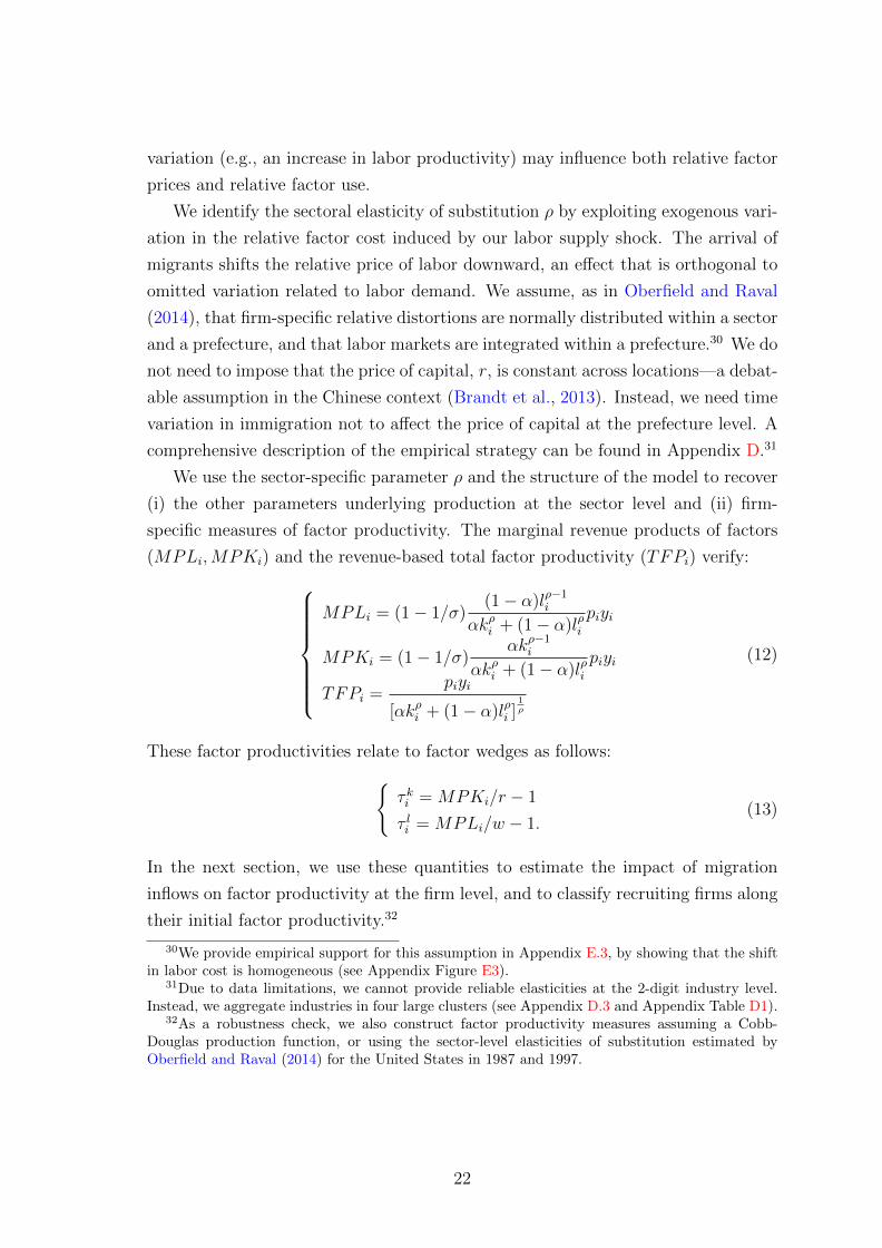
We use the sector-specific parameter ρ and the structure of the model to recover
(i) the other parameters underlying production at the sector level and (ii) firm-
specific measures of factor productivity. The marginal revenue products of factors
(MPLi,MPKi) and the revenue-based total factor productivity (TFPi) verify:
MPLi = (1− 1/σ)(1− α)lρ−1
i
αkρi + (1− α)lρipiyi
MPKi = (1− 1/σ)αkρ−1
i
αkρi + (1− α)lρipiyi
TFPi =piyi
[αkρi + (1− α)lρi ]1ρ
(12)
These factor productivities relate to factor wedges as follows:{τ ki = MPKi/r − 1
τ li = MPLi/w − 1.(13)
In the next section, we use these quantities to estimate the impact of migration
inflows on factor productivity at the firm level, and to classify recruiting firms along
their initial factor productivity.32
30We provide empirical support for this assumption in Appendix E.3, by showing that the shiftin labor cost is homogeneous (see Appendix Figure E3).
31Due to data limitations, we cannot provide reliable elasticities at the 2-digit industry level.Instead, we aggregate industries in four large clusters (see Appendix D.3 and Appendix Table D1).
32As a robustness check, we also construct factor productivity measures assuming a Cobb-Douglas production function, or using the sector-level elasticities of substitution estimated byOberfield and Raval (2014) for the United States in 1987 and 1997.
22
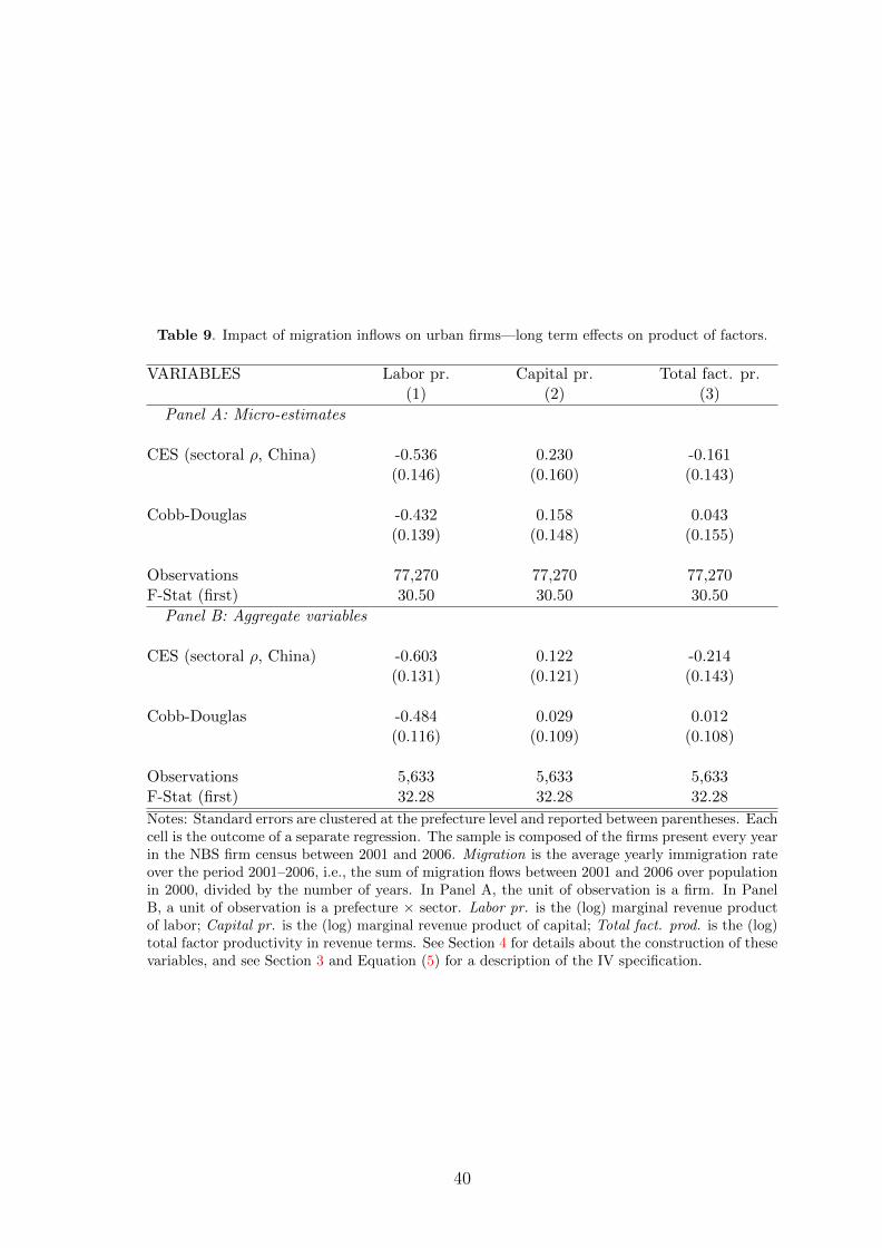
4.2 The effect of migration on factor productivity
Average effect We first study the impact of labor inflows on factor productivity
at the firm level. We estimate Equation (5) using the marginal revenue product of
labor, marginal revenue product of capital and total factor productivity in revenue
terms as dependent variables (all in logs). The estimates are presented in Table 9 for
the following production functions: the baseline CES production function with our
own sectoral estimates of ρ and the Cobb-Douglas specification, which corresponds to
the limiting case where ρ is zero. The first column of Table 9 (Panel A) reports how
marginal return to labor responds to migrant inflows. The elasticity with respect
to migration is about −0.54. In parallel, the marginal revenue product of capital
positively responds to the labor supply shift, as apparent from the second column
of Table 9. Finally, we find a small and non-significant negative effect of migration
on total factor productivity (see column 3).
These findings are inconsistent with a theoretical framework assuming optimiza-
tion under constant firm-specific distortions (see Equation 13). In this benchmark,
the magnitude of the decline in labor productivity would be similar to that of the la-
bor cost (−0.30, see Table 4), and capital productivity and total factor productivity
would remain stable. Instead, the gap between the marginal product of labor and
its marginal cost slightly decreases with immigrant inflows, and capital productivity
slightly increases.33 Firms become too labor-abundant in prefectures experiencing
large migrant inflows, which may hint at difficult access to capital.
The second row of Table 9 shows that a Cobb-Douglas production fails to cap-
ture these effects and underestimates the decrease in labor productivity. Capital
and labor are more complementary than what a Cobb-Douglas production function
would imply; the arrival of immigrants without further capitalization thus strongly
affects labor productivity.34
Heterogeneity analysis We now investigate the distributional effects of migrant
inflows. We classify firms based on (i) their marginal product of labor, (ii) marginal
product of capital and (iii) revenue-based total factor productivity at baseline (in
33Our framework assumes that labor is homogeneous, which implies that there is no productivitydifference between migrant and resident workers. Any discrepancy between the productivity ofurban residents and rural-to-urban migrants would generate a bias in the estimated effect of migrantinflows on factor productivity. We show in Appendix D.4 that, under reasonable assumptions aboutthe relative efficiency of migrant labor, this bias would however only account for a very small partof the decrease in labor productivity and increase in capital productivity.
34Appendix Table E6 shows that the productivity effects are similar when we use U.S. estimatesfor the CES parameters (Oberfield and Raval, 2014). These estimates also point to a highercomplementarity between capital and labor than induced by a Cobb-Douglas framework.
23
2001), and we construct a dummy equal to 1 if a firm is in the top quartile of its
sector × prefecture for each productivity measure. We interact migrant inflows with
each productivity dummy (see Equation 6), and report estimates of the employment
effect in Table 10.
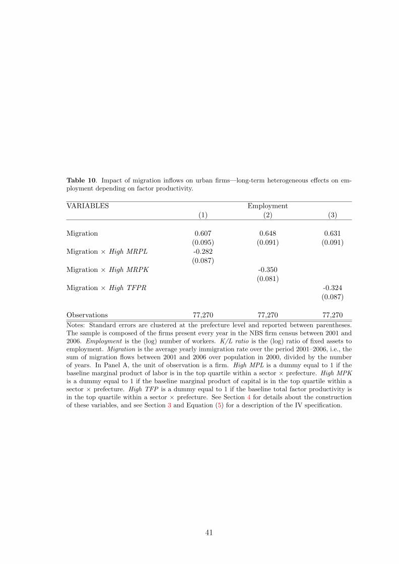
Immigrants are primarily recruited by manufacturing firms with low marginal
product of labor: Employment in low-productivity firms increases by 0.60% following
a one percentage point increase in the immigration rate, as against 0.32% in high-
productivity firms (column 1). The same result holds for capital productivity and
total factor productivity (columns 2 and 3): Hiring firms are unproductive firms.
This observation has implications for aggregate factor productivity at destination.
Labor inflows influence aggregate factor productivity through a direct effect, but
also through possible differences between the average employer and the marginal
employer—the recipient of migrant inflows. Immigrants being primarily hired by
unproductive firms, we should observe a negative compositional effect.
To show how the correlation between baseline factor productivity and employ-
ment growth affects aggregate productivity dynamics, we collapse factors and output
at the sector × prefecture level and create aggregate measures of factor productivity.
We then estimate a specification similar to Equation (4) where each observation is a
sector × prefecture in a given year. The aggregate elasticities of factor productivity
to migrant inflows are reported in Table 9 (Panel B). Following a one percentage
point increase in the immigration rate, changes in factor productivity appear to be
consistently more negative with aggregate measures than at the firm level (with dif-
ferences ranging between -0.05 and -0.12%). The systematic bias between Panels A
and B of Table 9 is consistent with the observed productivity differences between
the average and marginal employers, and is the most pronounced for capital pro-
ductivity.
Interpretation The interpretation of our findings depends on the nature of pro-
ductivity differences across firms within location and sector. In the spirit of the
model, firms in the same sector and location are perfectly identical except for (con-
stant) factor wedges, which capture unequal access to factor markets as in Hsieh
and Klenow (2009). Labor productivity dispersion would reflect labor market im-
perfections: firms with high marginal product of labor are constrained in hiring
labor. Our finding that firms with low marginal product of labor expand the most
following a migration inflow points towards a growing misallocation of labor at des-
tination. This misallocation may be due to information asymmetry between job
seekers and employers (Abebe et al., 2016; Alfonsi et al., 2017), to the intervention
24
of intermediaries and to the prevalence of migrant networks (Munshi, 2003; Barwick
et al., 2018). Similarly, capital productivity dispersion is indicative of capital mar-
ket distortions: firms with harder credit constraints have higher productivity than
the median firm in their sector and location (Buera et al., 2011; Midrigan and Xu,
2014). Our finding that firms become too labor-abundant, given the complemen-
tarities between capital and labor, suggests that capital constraints are even more
binding following a migrant inflow. Finally, productivity differences may capture
inherent entrepreneur characteristics, management practices (Bloom et al., 2013) or
differences in the organization of production (Akcigit et al., 2016; Boehm and Ober-
field, 2018). Better entrepreneurs or organizations would be captured by high total
factor productivity within a sector. Our finding that employment expands more in
firms with low total factor productivity would then suggest that migration benefits
more to firms whose management is of lower quality. In this case, again, our results
would indicate that migration worsens factor allocation within locations.
The previous interpretation of our results relies on the hypothesis that sector-
level estimates are a valid representation of production patterns in each firm. Any
deviation from this benchmark would be captured by firm-specific factor wedges.
For example, factor wedges may reflect technological differences across firms within
sectors due to firm-specific complementarities in production, or complementarities
in production with unobserved factors (e.g., skilled labor). A convincing normative
analysis would require us to estimate production at a more disaggregated level,
explicitly model factor market distortions, their interaction with labor supply and
their impact on firm dynamics, which is beyond what our data would permit. In the
next section, we show the implications of our findings on the allocation of factors
across locations.
4.3 Counterfactual experiment
As highlighted in the development literature (Lewis, 1954), migration should affect
the growth pattern of the manufacturing sector in cities and help bridge the gap
in factor productivity between locations. Our causal estimates of the effect of im-
migration can help us shed light on these questions. We combine (i) the observed
(selective) migration flows towards more or less booming locations and (ii) our causal
estimates of these flows at destination. This allows us to compare the growth rate
and dispersion of key characteristics of the Chinese manufacturing sector in two sce-
narios: the actual economy, and a counterfactual scenario without any migration.35
35Firm characteristics in the counterfactual scenario are obtained by subtracting the long-termcausal effects of migration, i.e., the coefficients reported in Table 4 multiplied by the migration
25
Growth Column 1 of Table 11 presents the annual growth rates of labor cost
(Panel A), relative factor use (Panel B), and factor productivity (Panels C and
D) in the actual economy and the counterfactual “no-migration” economy. Each
year, the urban economy becomes 6% more capital-abundant. However, the capital-
to-labor ratio would have grown even faster in the absence of migration—about
19% per year. The impact of migrants on relative factor use has implications for the
growth in labor cost and factor productivity. In the counterfactual economy without
migration, wage and labor productivity growth would have been almost twice as
large as in the actual economy (22 and 23%, against 13 and 14%). By contrast, the
growth of capital productivity would have been negative. Hence, migration played
an important role in the development of the manufacturing sector by slowing down
the secular increase in labor cost and rapid capitalization of manufacturing firms.
Dispersion The most interesting consequence of migration however lies in the
dispersion of factors and factor productivity across destinations. We report in col-
umn 2 of Table 11 the standard deviation of the outcomes in 2006, normalized by
the standard deviation in 2001. The dispersion in labor cost across firms decreased
by about 14% between 2001 and 2006 (Panel A). Migration markedly contributed
to this equalization of labor costs across production units: in the counterfactual
economy, the dispersion in labor costs would have increased by 14%. Along the
same lines, migration contributed to a moderate equalization of relative factor use
(Panel B) and factor productivity (Panels C and D) across firms. These modest
effects on total dispersion conceal a major impact of migration on dispersion across
prefectures (see columns 3 and 4 for the within and between standard deviations).
This finding illustrates that migrants do not select destinations at random; there is
a selective and systematic migration toward destinations where manufacturing firms
are capital-abundant, productive and paying high wages.
The allocative properties of rural-to-urban migration seem vastly different, when
studied within a destination or across locations. The absorption of migrant workers
by the manufacturing sector tends to worsen the allocation of factors within desti-
nations, thereby indicating significant distortions in capital and labor markets. In
this section, we have shown that the large and secular movement of workers across
locations significantly reduces productivity gaps between Chinese cities.
rate in each destination over the period.
26
5 Conclusion
This paper provides unique evidence on the causal effect of rural-urban migration on
manufacturing production in China. The analysis combines information on migra-
tion flows from population censuses with longitudinal data on manufacturing firms
between 2001 and 2006, a period of rapid structural transformation and sustained
manufacturing growth. We instrument migrant inflows using migration predictions
based on shocks at origin, i.e., the interaction of international price shocks for agri-
cultural commodities, cropping patterns and historical migration patterns between
rural areas and cities.
We leverage micro data by estimating the effect on factor use and factor cost
in the average firm. We find that migration decreases labor costs and increase em-
ployment in manufacturing. Manufacturing production expands but becomes more
labor-intensive, as capital does not adjust, even in the medium run. Labor produc-
tivity falls sharply. A quantitative framework suggests that labor allocation worsens
following a migration shock: recruiting firms have lower productivity than other
firms in the same sector and location. Productivity differences could also reflect
unobserved heterogeneity in capital constraints, product quality or technology: our
results suggest that production becomes too labor-abundant and migration favors
firms with labor-intensive production. Finally, we perform a counterfactual analy-
sis to quantify the role of migration in productivity growth and dispersion across
and within locations. While migration slows down productivity growth, it strongly
contributes to the equalization of factor productivity and wages across prefectures.
A limitation of our analysis is that we cannot provide evidence on labor market
frictions responsible for the observed factor reallocation due to the arrival of rural
migrants. Worker sorting across firms and sectors is likely driven by formal or
informal actors (e.g., recruiters or migrant networks), and depends on worker skills,
which we do not observe. We leave this for future work.
27
References
Abebe, Girum, Stefano Caria, Marcel Fafchamps, Paolo Falco, Simon Franklin,and Simon Quinn, “Anonymity or Distance? Job Search and Labour Market Exclu-sion in a Growing African City,” CSAE Working Paper Series 2016.
Accetturo, Antonio, Matteo Bugamelli, and Andrea Roberto Lamorgese, “Wel-come to the machine: firms’ reaction to low-skilled immigration,” Bank of Italy WorkingPaper, 2012, 846.
Akcigit, Ufuk, Harun Alp, and Michael Peters, “Lack of selection and limits todelegation: firm dynamics in developing countries,” Technical Report, National Bureauof Economic Research 2016.
Alfonsi, Livia, Oriana Bandiera, Vittorio Bassi, Robin Burgess, Imran Rasul,Munshi Sulaiman, and Anna Vitali, “Tackling Youth Unemployment: Evidencefrom a Labour Market Experiment in Uganda,” Technical Report 64, STICERD, LSEDecember 2017.
Alvarez-Cuadrado, Francisco and Markus Poschke, “Structural Change Out ofAgriculture: Labor Push versus Labor Pull,” American Economic Journal: Macroeco-nomics, July 2011, 3 (3), 127–58.
Angelucci, Manuela, “Migration and Financial Constraints: Evidence from Mexico,”The Review of Economics and Statistics, March 2015, 97 (1), 224–228.
Badaoui, Eliane El, Eric Strobl, and Frank Walsh, “Impact of Internal Migrationon Labor Market Outcomes of Native Males in Thailand,” Economic Development andCultural Change, 2017, 66, 147–177.
Banerjee, Abhijit V. and Esther Duflo, “Do Firms Want to Borrow More? TestingCredit Constraints Using a Directed Lending Program,” Review of Economic Studies,2014, 81 (2), 572–607.
Barwick, Panle Jia, Yanyan Liu, Eleonora Patacchini, and Qi Wu, “Information,Mobile Communication Patterns and Social Referrals,” Technical Report 2018.
Bazzi, Samuel, “Wealth heterogeneity and the income elasticity of migration,” AmericanEconomic Journal: Applied Economics, 2017, 9 (2), 219–55.
Bloom, Nicholas, Benn Eifert, Aprajit Mahajan, David McKenzie, and JohnRoberts, “Does management matter? Evidence from India,” The Quarterly Journalof Economics, 2013, 128 (1), 1–51.
Boehm, Johannes and Ezra Oberfield, “Misallocation in the Market for Inputs: En-forcement and the Organization of Production,” Technical Report, National Bureau ofEconomic Research 2018.
Borjas, George J., “The Labor Demand Curve Is Downward Sloping: Reexamining TheImpact Of Immigration On The Labor Market,” The Quarterly Journal of Economics,November 2003, 118 (4), 1335–1374.
28
Boustan, Leah Platt, Price V. Fishback, and Shawn Kantor, “The Effect of Inter-nal Migration on Local Labor Markets: American Cities during the Great Depression,”Journal of Labor Economics, October 2010, 28 (4), 719–746.
Brandt, Loren, Gueorgui Kambourov, and Kjetil Storesletten, “Firm Entry andRegional Growth Disparities: the Effect of SOEs in China,” University of Torontomimeo, 2016.
, Johannes Van Biesebroeck, and Yifan Zhang, “Creative accounting or creativedestruction? Firm-level productivity growth in Chinese manufacturing,” Journal ofDevelopment Economics, 2012, 97 (2), 339–351.
, , and , “Challenges of working with the Chinese NBS firm-level data,” ChinaEconomic Review, 2014, 30 (C), 339–352.
, Trevor Tombe, and Xiaodong Zhu, “Factor market distortions across time, spaceand sectors in China,” Review of Economic Dynamics, 2013, 16 (1), 39–58.
Bryan, Gharad and Melanie Morten, “Economic Development and the Spatial Allo-cation of Labor: Evidence from Indonesia,” Technical Report 2015.
Buera, Francisco J, Joseph P Kaboski, and Yongseok Shin, “Finance and de-velopment: A tale of two sectors,” The American Economic Review, 2011, 101 (5),1964–2002.
Bustos, Paula, Bruno Caprettini, and Jacopo Ponticelli, “Agricultural productiv-ity and structural transformation: Evidence from Brazil,” American Economic Review,2016, 106 (6), 1320–65.
Card, David, “Immigrant Inflows, Native Outflows, and the Local Labor Market Impactsof Higher Immigration,” Journal of Labor Economics, 2001, 19 (1), 22–64.
and John DiNardo, “Do Immigrant Inflows Lead to Native Outflows?,” AmericanEconomic Review, 2000, 90 (2), 360–367.
Chan, Kam Wing and Will Buckingham, “Is China abolishing the hukou system?,”The China Quarterly, 2008, 195, 582–606.
Cole, William E and Richard D Sanders, “Internal migration and urban employmentin the Third World,” The American Economic Review, 1985, 75 (3), 481–494.
Combes, Pierre-Philippe, Sylvie Demurger, and Shi Li, “Migration externalitiesin Chinese cities,” European Economic Review, 2015, 76 (C), 152–167.
Davis, Steven J and John C Haltiwanger, “Job creation and destruction,” MIT PressBooks, 1998, 1.
Demurger, Sylvie, Marc Gurgand, Shi Li, and Ximing Yue, “Migrants as second-class workers in urban China? A decomposition analysis,” Journal of ComparativeEconomics, December 2009, 37 (4), 610–628.
Dustmann, Christian and Albrecht Glitz, “How Do Industries and Firms Respond toChanges in Local Labor Supply?,” Journal of Labor Economics, 2015, 33 (3), 711–750.
29
Ebenstein, Avraham and Yaohui Zhao, “Tracking rural-to-urban migration in China:Lessons from the 2005 inter-census population survey,” Population Studies, 2015, 69 (3),337–353.
Facchini, Giovanni, Maggie Y. Liu, Anna Maria Mayda, and Minghai Zhou,“The impact of China’s WTO accession on internal migration,” 2015.
Fan, Cindy C., China on the Move, Routledge, 2008.
Feng, Shuaizhang, Yingyao Hu, and Robert Moffitt, “Long run trends in unemploy-ment and labor force participation in urban China,” Journal of Comparative Economics,2017, 45 (2), 304 – 324.
Fields, Gary S, “Rural-urban migration, urban unemployment and underemployment,and job-search activity in LDCs,” Journal of development economics, 1975, 2 (2), 165–187.
Franklin, Simon, “Location, Search Costs and Youth Unemployment: ExperimentalEvidence from Transport Subsidies,” Economic Journal, September 2018, 128 (614),2353–2379.
Ge, Suqin and Dennis Tao Yang, “Changes In China’s Wage Structure,” Journal ofthe European Economic Association, 04 2014, 12 (2), 300–336.
Giulietti, Corrado, Guangjie Ning, and Klaus F Zimmermann, “Self-employmentof rural-to-urban migrants in China,” International Journal of Manpower, 2012, 33 (1),96–117.
Gollin, Douglas, David Lagakos, and Michael E. Waugh, “The Agricultural Pro-ductivity Gap,” The Quarterly Journal of Economics, 2014, 129 (2), 939–993.
, Stephen Parente, and Richard Rogerson, “The Role of Agriculture in Develop-ment,” American Economic Review, May 2002, 92 (2), 160–164.
Gopinath, Gita, Sebnem Kalemli-Ozcan, Loukas Karabarbounis, and CarolinaVillegas-Sanchez, “Capital allocation and productivity in South Europe,” The Quar-terly Journal of Economics, 2017, 132 (4), 1915–1967.
Groger, Andre and Yanos Zylberberg, “Internal Labor Migration as a Shock CopingStrategy: Evidence from a Typhoon,” American Economic Journal: Applied Economics,April 2016, 8 (2), 123–53.
Harris, John R. and Michael P. Todaro, “Migration, Unemployment and Devel-opment: A Two-Sector Analysis,” The American Economic Review, 1970, 60 (1), pp.126–142.
Herrendorf, Berthold, Christopher Herrington, and Akos Valentinyi, “SectoralTechnology and Structural Transformation,” Technical Report 9386, C.E.P.R. Discus-sion Papers 2013.
Hsieh, Chang-Tai and Peter J. Klenow, “Misallocation and Manufacturing TFPin China and India,” The Quarterly Journal of Economics, November 2009, 124 (4),1403–1448.
30
and Zheng Song, “Grasp the Large, Let Go of the Small: The Transformation of theState Sector in China,” NBER Working Papers 21006, National Bureau of EconomicResearch, Inc March 2015.
Imbert, Clement and John Papp, “Short-term Migration, Rural Workfare Programsand Urban Labor Markets: Evidence from India,” The Warwick Economics ResearchPaper Series (TWERPS) 1116 2016.
Kerr, Sari Pekkala, William R. Kerr, and William F. Lincoln, “Skilled Immigra-tion and the Employment Structures of US Firms,” Journal of Labor Economics, 2015,33 (S1), S147 – S186.
Kinnan, Cynthia, Shing-Yi Wang, and Yongxiang Wang, “Access to Migration forRural Households,” American Economic Journal: Applied Economics, 2017.
Kleemans, Marieke and Jeremy Magruder, “Labour Market Responses To Immigra-tion: Evidence From Internal Migration Driven By Weather Shocks,” Economic Journal,August 2018, 128 (613), 2032–2065.
Lewis, Arthur, “Economic Development with Unlimited Supplies of Labour,” TheManchester School, 1954, 22 (2), 139–191.
Lewis, Ethan, “Immigration, Skill Mix, and Capital Skill Complementarity,” The Quar-terly Journal of Economics, 2011, 126 (2), 1029–1069.
Llull, Joan, “Immigration, Wages, and Education: A Labour Market Equilibrium Struc-tural Model,” The Review of Economic Studies, 2018, 85 (3), 1852–1896.
Mayneris, Florian, Sandra Poncet, and Tao Zhang, “The cleansing effect of min-imum wages. Minimum wages, firm dynamics and aggregate productivity in China,”Core Discussion Papers 2014/44 October 2014.
Meghir, Costas, Renata Narita, and Jean-Marc Robin, “Wages and informality indeveloping countries,” American Economic Review, 2015, 105 (4), 1509–46.
Meng, Xin and Dandan Zhang, “Labour Market Impact of Large Scale Internal Mi-gration on Chinese Urban ’Native’ Workers,” IZA Discussion Papers 5288 October 2010.
Midrigan, Virgiliu and Daniel Yi Xu, “Finance and misallocation: Evidence fromplant-level data,” The American Economic Review, 2014, 104 (2), 422–458.
Minale, Luigi, “Agricultural productivity shocks, labour reallocation and rural-urbanmigration in China,” Journal of Economic Geography, 2018, p. lby013.
Monras, Joan, “Immigration and Wage Dynamics: Evidence from the Mexican PesoCrisis,” Working Papers hal-01127022, HAL March 2015.
, “Economic Shocks and Internal Migration,” CEPR Discussion Papers 12977, C.E.P.R.Discussion Papers June 2018.
Munshi, Kaivan, “Networks in the modern economy: Mexican migrants in the US labormarket,” The Quarterly Journal of Economics, 2003, 118 (2), 549–599.
Oberfield, Ezra and Devesh Raval, “Micro data and macro technology,” 2014.
31
Olney, William W, “Immigration and firm expansion,” Journal of Regional Science,2013, 53 (1), 142–157.
Park, Albert, “Rural-urban inequality in China,” in Shahid Yusuf and Karen Nabeshima,eds., China Urbanizes: Consequences, Strategies, and Policies, The World Bank, 2008.
Peri, Giovanni, “The Effect Of Immigration On Productivity: Evidence From U.S.States,” The Review of Economics and Statistics, February 2012, 94 (1), 348–358.
Santangelo, Gabriella, “Firms and Farms: The Impact of Agricultural Productivity onthe Local Indian Economy,” 2016. Manuscript.
Satchi, Mathan and Jonathan Temple, “Labor markets and productivity in develop-ing countries,” Review of Economic dynamics, 2009, 12 (1), 183–204.
Song, Yang, “What should economists know about the current Chinese hukou system?,”China Economic Review, 2014, 29, 200–212.
Song, Zheng, Kjetil Storesletten, and Fabrizio Zilibotti, “Growing Like China,”American Economic Review, 2011, 101 (1), 196–233.
Sousa, Jose De and Sandra Poncet, “How are wages set in Beijing?,” Regional Scienceand Urban Economics, 2011, 41 (1), 9–19.
Todaro, Michael, “Internal Migration in Developing Countries: A Survey,” in “Popula-tion and Economic Change in Developing Countries” NBER Chapters, National Bureauof Economic Research, 1980, pp. 361–402.
Todaro, Michael P, “A model of labor migration and urban unemployment in lessdeveloped countries,” The American economic review, 1969, 59 (1), 138–148.
Tombe, Trevor and Xiaodong Zhu, “Trade, Migration and Productivity: A Quanti-tative Analysis of China,” June 2015.
Ulyssea, Gabriel, “Firms, Informality, and Development: Theory and Evidence fromBrazil,” American Economic Review, August 2018, 108 (8), 2015–47.
Zhang, Junfu and Zhong Zhao, “Social-family network and self-employment: evidencefrom temporary rural–urban migrants in China,” IZA Journal of Labor & Development,2015, 4 (1), 4.
Zhang, Li and Li Tao, “Barriers to the acquisition of urban hukou in Chinese cities,”Environment and Planning A, 2012, 44 (12), 2883–2900.
32
Figures and tables
Figure 1. Potential output in China for rice and cotton (2000).
(a) Paddy rice. (b) Cotton.
Notes: These maps represent the potential output constructed from interacting harvested areas (2000) and potentialyield (GAEZ model) for two common crops in China, i.e., paddy rice (left panel) and cotton (right panel).
Figure 2. Distribution of revenue across firms (NBS, 2001–2006).
Sources: Firm-level data from the National Bureau of Statistics (NBS), 2001–2006. The revenue threshold forappearing in the NBS Census of above-scale firms is RMB 5,000,000, corresponding to ln(5, 000) ≈ 8.52 along thelogarithmic scale (of revenues expressed in thousands of RMB).
Notes: Standard errors are clustered at the prefecture level and reported between parentheses. InPanel A, the dependent variable is the number of rural emigrants to urban areas in other prefecturesor in prefectures located outside of a 300-km radius around the origin, divided by the number ofrural residents at origin. In Panel B, the dependent variable is the number of rural immigrantsfrom other prefectures or prefectures located outside of a 300-km radius around the destinationdivided by the number of urban residents at destination. See Section 2 and Equations (2) and (3)for a more comprehensive description of the two specifications.
Table 2. Summary statistics of key firm-level outcomes.
Standard deviationMean total within between
Labor Cost 2.52 0.64 0.41 0.49Employment 5.16 1.08 0.34 1.03K/L Ratio 3.88 1.10 0.43 1.01Y/L Ratio 3.74 0.95 0.54 0.78
Sources: NBS firm-level data (2001). The sample includes the 77,270 firms used in the baselinespecification (4). Labor cost is the (log) compensation per worker including social security. Em-ployment is the (log) number of workers. K/L ratio is the (log) ratio of fixed assets (in thousandyuan) to employment. Y/L ratio is the (log) ratio of value added to employment. The first andsecond columns present the mean and standard deviation of the key outcome variables. The thirdand fourth columns report the standard deviation within and across prefectures.
34
Table 3. Impact of migration inflows on urban firms—short run effects.
Notes: Standard errors are clustered at the prefecture level and reported between parentheses. Thesample is composed of the firms present every year in the NBS firm census between 2001 and 2006.Migration is the immigration rate, i.e., the migration flow divided by destination population atbaseline. Labor cost is the (log) compensation per worker including social security. Employmentis the (log) number of workers. K/L ratio is the (log) ratio of fixed assets to employment. Y/Lratio is the (log) ratio of value added to employment. All specifications include firm and year fixedeffects. See Section 2 and Equation (4) for a description of the IV specification.
35
Table 4. Impact of migration inflows on urban firms—long run effects.
Notes: Standard errors are clustered at the prefecture level and reported between parentheses.The sample is composed of the firms present every year in the NBS firm census between 2001 and2006. Migration is the average yearly immigration rate over the period 2001–2006, i.e., the sum ofmigration flows between 2001 and 2006 over population in 2000, divided by the number of years.Labor cost is the (log) compensation per worker including social security. Employment is the (log)number of workers. K/L ratio is the (log) ratio of fixed assets to employment. Y/L ratio is the(log) ratio of value added to employment. See Section 3 and Equation (5) for a description of theIV specification.
Table 5. Impact of migration inflows on urban firms—heterogeneous effects.
Notes: Standard errors are clustered at the prefecture level and reported between parentheses.The sample is composed of the firms present every year in the NBS firm census between 2001 and2006. High K/L is a dummy equal to 1 if the baseline capital-to-labor ratio belongs to the topquartile within the industry/prefecture. High Y/L is a dummy equal to 1 if the baseline valueadded-to-labor ratio belongs to the top quartile within the industry/prefecture. All specificationsinclude firm and year fixed effects. See Section 2 and Equation (6) for a description of the IVspecification.
36
Table 6. Impact of migration inflows on urban firms—sensitivity analysis.
Notes: Standard errors are clustered at the prefecture level and reported between parentheses.The sample is composed of the firms present every year in the NBS firm census between 2001 and2006. All specifications include firm and year fixed effects. See Section 2 and Equation (4) for adescription of the IV specification.
37
Table 7. Impact of migration inflows on urban firms—sensitivity analysis with aggregate variablesat the prefecture × sector level.
Notes: Standard errors are clustered at the prefecture level and reported between parentheses. Theunit of observation is a prefecture × sector in a given year. In Panel A (resp. Panel B), the sampleis composed of the firms present every year in the NBS firm census between 2001 and 2006 (resp.all firms present in the NBS firm census between 2001 and 2006); outcomes are then aggregatedat the prefecture × sector level. Migration is the immigration rate, i.e., the migration flow dividedby destination population at baseline. Labor cost is the (log) compensation per worker includingsocial security. Employment is the (log) number of workers within the firm. K/L ratio is the (log)ratio of fixed assets to employment. Y/L ratio is the (log) ratio of value added to employment.All specifications include prefecture × sector and year fixed effects.
38
Table 8. Impact of migration inflows on urban residents.
Notes: Standard errors are clustered at the prefecture level and reported between parentheses.Low Skill is defined as a dummy equal to 1 for workers with no education, primary education orlower secondary education. Wage is the (log) hourly wage in real terms. Employee is a dummy forreceiving a wage, while Self-employed is a dummy equal to 1 for individuals who are self-employedor employers. All specifications include year and prefecture fixed effects. † The IV specificationuses two endogenous variables and two instruments; the critical value for weak instruments is then7.03 (at 10%).
39
Table 9. Impact of migration inflows on urban firms—long term effects on product of factors.
VARIABLES Labor pr. Capital pr. Total fact. pr.(1) (2) (3)
Panel A: Micro-estimates
CES (sectoral ρ, China) -0.536 0.230 -0.161(0.146) (0.160) (0.143)
Notes: Standard errors are clustered at the prefecture level and reported between parentheses. Eachcell is the outcome of a separate regression. The sample is composed of the firms present every yearin the NBS firm census between 2001 and 2006. Migration is the average yearly immigration rateover the period 2001–2006, i.e., the sum of migration flows between 2001 and 2006 over populationin 2000, divided by the number of years. In Panel A, the unit of observation is a firm. In PanelB, a unit of observation is a prefecture × sector. Labor pr. is the (log) marginal revenue productof labor; Capital pr. is the (log) marginal revenue product of capital; Total fact. prod. is the (log)total factor productivity in revenue terms. See Section 4 for details about the construction of thesevariables, and see Section 3 and Equation (5) for a description of the IV specification.
40
Table 10. Impact of migration inflows on urban firms—long-term heterogeneous effects on em-ployment depending on factor productivity.
Notes: Standard errors are clustered at the prefecture level and reported between parentheses.The sample is composed of the firms present every year in the NBS firm census between 2001 and2006. Employment is the (log) number of workers. K/L ratio is the (log) ratio of fixed assets toemployment. Migration is the average yearly immigration rate over the period 2001–2006, i.e., thesum of migration flows between 2001 and 2006 over population in 2000, divided by the numberof years. In Panel A, the unit of observation is a firm. High MPL is a dummy equal to 1 if thebaseline marginal product of labor is in the top quartile within a sector × prefecture. High MPKis a dummy equal to 1 if the baseline marginal product of capital is in the top quartile within asector × prefecture. High TFP is a dummy equal to 1 if the baseline total factor productivity isin the top quartile within a sector × prefecture. See Section 4 for details about the constructionof these variables, and see Section 3 and Equation (5) for a description of the IV specification.
41
Table 11. Counterfactual experiment—effects of migration on wages, factor use and factor pro-ductivity (growth and dispersion).
Annual growth Standard deviation (2006/2001)(2001–2006) all within pref. betw. pref.
Notes: In the counterfactual scenario (No migration), we set the immigration rates equal to 0 inevery prefecture and every year between 2001 and 2006. Column 1 reports the average annualgrowth rate between 2001 and 2006 under the different scenarios. Column 2 reports the standarddeviation of the variable of interest in 2006 normalized by its standard deviation in 2001; columns3 and 4 replicates this exercise with the separate between- and within-components.
42
ONLINE APPENDIX
A Migration flows: construction and description 44
In this section, we provide elements of context about migration in China, focusing
on the hukou system and its implementation over time and across provinces. We
describe the construction of migration flows from retrospective questions, and the
adjustment accounting for return migration. Finally, we discuss key descriptive
statistics.
A.1 Elements of context
An important feature of China’s society is the division of the population accord-
ing to its household registration or hukou status.36 Chinese citizens are classified
along two dimensions: their hukou type (hukou xingzhi)—agricultural (nongye) or
non-agricultural (fei nongye)—and hukou location (hukou suozaidi). Both charac-
teristics, recorded in the household registration booklet, may not correspond to the
actual occupation and location.
Since the inception of the reforms in the late 1970s, rules regarding migra-
tion within China have been relaxed. Labor mobility remains subject to legal
requirements—e.g., being lawfully employed at destination—but the large flows of
internal migrants that have characterized China’s recent development show that
barriers are low in practice, at least for individual (as opposed to family) migra-
tion. Migrants however seldom gain local registration status and do not enjoy the
same rights as the locally registered population. This is likely to impede mobility,
to reduce migrant workers’ bargaining power and to lock migrants in a position
of “second-class workers” (Demurger et al., 2009). Whereas an agricultural hukou
grants access to land, non-agricultural hukou holders enjoy public services in their
cities of registration. We focus below on the challenges faced by agricultural hukou
holders settling in urban areas.
The type and place of registration have far-reaching consequences. Access to
welfare benefits and public services (e.g., enrollment in local schools, access to health
care, urban pension plans and subsidized housing) is conditional on being officially
recorded as a local urban dweller. Subsequently, migrants face a high cost of living in
cities and are supposed to return to their places of registration for basic services such
as education and health care or they are charged higher fees (Song, 2014). Labor
outcomes are also affected as local governments may issue regulations restricting
access to job opportunities or rely on informal guidelines to employers to favor local
permanent residents. As it became possible for state-owned enterprises (SOEs) to
36This subsection draws partly on Chan and Buckingham (2008).
44
lay off “permanent workers” in the 1990s, regulations were introduced to bar them
from employing migrant labor instead (Demurger et al., 2009).
Despite the rigidity of the hukou system and the persistently low rate of hukou
conversion, reforms have progressively been introduced during the structural trans-
formation of China. Since the 1980s, China has experienced a gradual devolution of
power from the central to local governments in terms of hukou policy and manage-
ment. As a consequence, rules and implementation vary substantially across places
and over time. Provincial governments typically set general guidelines and more
specific rules are then determined by prefectures, which in practice hold the most
power over hukou policy (Song, 2014). Two major reforms were introduced in re-
cent years. First, the distinction between agricultural and non-agricultural hukou
was abolished within local jurisdictions in about one third of Chinese provinces. Al-
beit an important evolution, this reform does not affect rural-to-urban migrants who
come from other prefectures, let alone different provinces. Second, hukou conversion
rules have been gradually loosened. The main channels to change one’s hukou from
agricultural to non-agricultural used to include recruitment by an SOE, receiving
college education or joining the army. These conditions have been relaxed since
2000, especially in small cities and towns that attract fewer migrants (Zhang and
Tao, 2012). In larger cities, however, conditions for eligibility are tough, so that
hukou conversion reforms primarily benefit the richest and highly educated (Song,
2014).
The identification strategy described in Section 2 allows us to deal with the
potential endogeneity of migration policy to local factor demand. The predicted,
supply-driven migration flows that are used as an instrument for actual flows in our
IV strategy are indeed orthogonal to such dynamics.
A.2 Data sources and construction of migration flows
Data description In order to measure migration flows, we use the 2000 Popula-
tion Census, the 2005 1% Population Survey, also called “2005 Mini-Census,” and
the 2010 Population Census.
After the beginning of the reforms and loosening of restrictions on mobility, there
was a growing disconnect between census data focusing on hukou location and the
rising “floating population” of non-locally registered citizens. The 2000 Population
Census was the first census to acknowledge this gap and record migrants’ place of
residence—provided they had been living there for more than 6 months (Ebenstein
and Zhao, 2015). In addition to the place of residence (at the prefecture level in our
data), hukou location (province level) and hukou type, the 2000 and 2010 Population
45
Censuses contain retrospective information on the place of residence 5 years before
the survey (province level) and the reason for departure if residence and registration
hukou do not coincide. The 2000 and 2010 Censuses slightly differ in how they
record migration: The 2000 (resp. 2010) Census records the year of arrival (resp.
departure), censored if migration happened 5 years or more before the interview,
and the 2000 (2010) Census provides information on the last prefecture of residence
before the move (the prefecture of hukou registration).
The 2005 1% Population Survey constitutes a 1.3% [sic] sample of the population
selected from 600,000 primary census enumeration districts thanks to a three-stage
cluster sampling (Ebenstein and Zhao, 2015). All Chinese counties (the level of
administration below prefectures) are covered. The sampling weights provided by
the National Bureau of Statistics (NBS) account for the underlying proportional
probability sampling scheme based on the 2004 population registry of the Public
Security Bureau.
A few caveats are in order. First, the sampling frame contained only information
on population by registration. High-immigration areas could thus be under-sampled.
Comparing the flows for 2005 in the 2005 Mini-Census and 2010 Census, we indeed
find a small discrepancy that we attribute to coverage issues. Second, the 2005 Mini-
Census offers a set of variables similar to standard censuses but some discrepancies
are worth bearing in mind: (i) Both data sources provide prefecture-level informa-
tion on the place of residence, but it is defined as “current residence” in 2005 and
thus also captures migrants who have been established at destination for less than 6
months. (ii) The 2000 Census contains prefecture-level information on the place of
residence prior to arrival at destination, while the 1% Survey records hukou location
at the prefecture level, just like the 2010 Census. These two places are one and
the same if there is no step migration, i.e., if rural dwellers move directly to their
final destinations. Along the same lines, the 2005 Mini-Census records the timing
of departure from a migrant’s place of registration rather than of arrival at destina-
tion. (iii) The data do not record the place of residence at high enough resolution
to unambiguously infer whether a migrant is residing in a rural or urban area. Nev-
ertheless, rural-to-rural migration represents a small share of emigration from rural
areas, mostly explained by marriage—which usually gives right to local registration
(Fan, 2008).37 (iv) We cannot account for migrants who changed their hukou lo-
cation or type. This assumption is quite innocuous given that hukou conversion is
marginal.
37In the 2005 Mini-Census, only 4.7% of agricultural hukou holders who migrated betweenprefectures reported having left their places of registration to live with their spouses after marriage.See Table A2 for further descriptive statistics on reasons for moving.
46
Migration flow construction The retrospective data on migration spells in the
two Censuses and Mini-Census allows us to construct yearly migration flows over
the period 1996–2010. These flows are directly observed rather than computed as a
difference of stocks as common in the migration literature.
We construct annual migration flows between all prefectures of origin and desti-
nation by combining information on the current place of residence (the destination),
the place of registration (the origin) and the year in which the migrant left the origin.
One advantage of working with those data is that they cover—or are representative
of—the whole population: All individuals, irrespective of their hukou status, were
interviewed in 2000, 2005 and 2010. However, not all migration spells are observed.
We describe below (i) which migration spells are directly observed and which spells
are omitted, and (ii) how we can infer some of the unobserved spells and adjust the
raw migration flows.
Not all migration spells are observed in the three censuses. We only observe
single migration spells, i.e., migration spells in which the interviewed individual is
at destination at the time of interview, and whose origin coincides with the hukou
location. For these individuals, the origin is deduced from their hukou location, and
the date of their unique relocation is available. All other types of migration histories
during the five years preceding the interview are less straightforward to identify.
For instance, if one individual were to leave her hukou location to city A in 2002
and then transit to city B in 2005, we would only record the last relocation. In such
step migration cases, we would correctly attribute arrival dates at destination for
the last spell but we would incorrectly attribute the departure time from origin in
the 2000 Census. In the 2005 Mini-Census and 2010 Census, we would incorrectly
attribute arrival dates at destination for the last spell, but we would correctly specify
the departure time from origin. In both data sets, we would miss arrival in city A. If,
instead, one individual were to leave her hukou location to city A in 2002 and then
return to her hukou location by 2005, we would miss her entire migration history. In
such return migration cases, we would incorrectly omit emigration flows from origins
and immigration to destinations.
The incidence of step migration and return migration spells can, however, be
measured. Indeed, the 2005 Mini-Census records where individuals were living 1 and
5 years before the survey (province level), while the 2000 and 2010 Censuses include
a question about the residence 5 years prior to the interview. We can estimate how
many migrants report different destinations between 2000 and 2005, which would
be a proxy for step migration, and we can observe total return migration between
1995 and 2000, 2000 and 2005, 2004 and 2005, and 2005 and 2010.
47
We first study the importance of step migration. Among all the migrants who
were in their provinces of registration in 2000 and in other provinces in 2005, we
compute the fraction that lived in yet another province in 2004. As Figure A1 shows,
only a minority of migrants have changed provinces of destination between 2003 and
2004. Step migration is not only small but also concentrated in the very first year
after the first migration spell. In other words, step migration induces errors in arrival
and departure dates that are also quite small. As adjusting for step migration would
require strong assumptions about the intermediate destination, which is not observed
in the data, we do not correct migration flows for step migration.
Figure A1. Share of step migrants as a function of age and time since departure.
Sources: 2005 1% Population Survey.
We then consider the extent of return migration. Among all migrants from rural
areas who were living in their provinces of registration in 2000 and in other provinces
in 2004, we compute the fraction that had returned to their provinces of registration
by 2005. This share is not negligible: In a given year, between 4 and 6% of rural
migrants who had left their provinces of registration in the last 6 years go back to
their hukou locations. Return migration is hence an important phenomenon, which
leads us to underestimate true migration flows and the effect of shocks on emigration.
Because of the retrospective nature of the data, past flows, for instance in 2000 for an
individual interviewed in 2005, are mechanically underestimated. In contrast with
step migration, however, it is possible—under reasonable assumptions—to adjust
migration flows and account for return migration. We provide below a description
48
of these adjustments.
Adjusting for return migration requires us to observe the destination and duration-
specific yearly rate of return. There is a wide disparity in return rates across destina-
tions. Besides, there are non-negligible compositional adjustments along the dura-
tion of the migration spell—as in any survival analysis with censoring. Specifically,
the probability for a migrant to return home sharply decreases with the length of
the migration spell, mostly reflecting heterogeneity across migrants in their propen-
sity to return. Ignoring such heterogeneity would lead us to underestimate return
migration for recent flows and overestimate it for longer spells.
To capture variation across destinations and along the length of the migration
spell, we make the following assumptions. (i) The “survival” at destination is char-
acterized by a constant Poisson rate f for each migrant. (ii) We suppose that there
is a constant distribution of migrant types H(f) upon arrival. We allow the distri-
butions to differ across provinces of destination and hukou types, i.e., agricultural
and non-agricultural. (iii) In order to fit the observed return rates as a function of
migration duration, we further assume that:
h(f) = λ2pfe
−λpf .
where λp is province- and hukou type-specific.
Under the previous assumptions and in a steady-state environment, the evolution
of the pool of migrants with duration can easily be computed. In the cross-section
(i.e., across all cohorts and not only newly-arrived migrants), the distribution of
migrant types is exponential, i.e., hc(f) = λpe−λpf , such that the average yearly
return rate is 1/λp. In all census waves, we observe the hukou location, the place of
residence five years before the survey and the place of residence during the survey.
This observation allows us to compute the empirical return rate in the cross-section
over a period of five years. We calibrate the hukou- and province-specific exponential
parameter λp to match this return rate, and we perform this calibration in each
wave such that we flexibly allow for long-term fluctuations in these province-specific
distributions.
Using the calibrated distribution H(·), we can infer the initial flow of migrants
from the number of survivors observed k years later and correct for return migration.
More precisely, letting MT,k denote the number of migrants arrived in period t =
T − k and recorded in period T , the actual number of newly-arrived migrants in
t = T − k is[(λp + k)2/λ2
p
]MT,k. We carry out this exercise for the 2000 Census,
the 2005 Mini-Census and the 2010 Census.
One concern with this methodology is that we may not precisely capture the
49
duration-dependence in return rates, and thus over- or underestimate return rates
for individuals arriving immediately before the interview. Using the 2005 Survey, we
provide an over-identification test by computing the return probability between 2004
and 2005 for recently-arrived migrants (i.e., between 2000 and 2004), and compare
it with the empirical moment. We compute this model-based probability under our
baseline specification (B) and under an alternative specification (R) where return
rates are assumed to be independent of duration.
Figure A2. Over-identification test for the return migration correction.
Sources: 2005 1% Population Survey.
Figure A2 displays the model-based return probabilities for recently-arrived mi-
grants against the actual observed return rate. The baseline specification (B, blue
dots) matches well the prefecture-level variation in annual return rate for recently-
arrived migrants, while the alternative specification (R, red dots) systematically
underestimates return. Under the alternative specification (R), the return rate af-
ter one year is about half the observed rate—a difference due to the fact that the
calibration then ignores the difference between the (high) return rate conditional on
a short migration spell and the (low) return rate conditional on longer spells. Note
that, even under specification (B), there is noise and some model-based estimates
are quite far from the actual return rates. This difference could be due to fluctua-
tions in return rates across years: While the calibration uses the 2000–2005 period,
the validation check focuses on 2004–2005 only.
50
A.3 Description
In this section, we provide descriptive statistics about migration flows and the se-
lection of migrants.
Migration patterns over time and across regions Migration patterns vary
both over time and across origins and destinations. First, there is a general in-
crease in migrant inflows during the period 1996–2010, probably related to the de-
cline in mobility costs and the attractiveness of new buoyant cities. We report in
Figure A3 the ratio of annual inter-prefecture migrant flows to the population regis-
tered in urban areas. The average annual inflow of migrants from other prefectures
is around 3% of the destination population. Figure A3 provides some information
about the nature of these migration spells. Migration is mostly rural-to-urban and
long-distance. Over the period 1996–2010, about 80% of the yearly migrant in-
flows consist of agricultural hukou holders (“rural” migrants), the remainder being
urban dwellers originating from other prefectures. About 80% of inter-prefectural
ruralto–urban migrations involve the crossing of a provincial border.
Figure A3. Evolution of migration rates between 1996 and 2010.
Sources: 2000 and 2010 Censuses, and 2005 Mini-Census.
There is a large variation in the spatial distribution of migration inflows and out-
flows (see Table A1). Some regions (e.g., East, South Central) are net recipients, and
attract a large share of local migrants, while some other regions (e.g., North-West)
51
are net senders. However, even if there is significant variation in terms of both
emigration and immigration rates across regions, no region is left aside from the
migration phenomenon. Moreover, conditional on originating from the same prefec-
ture, there is dispersion of migration spells across destinations. The bottom panel of
Table A1 displays the prefecture-level Herfindahl-Hirschmann Index of destination
concentration. Regions differ in terms of destination concentration but migrants
from any of the six main regions do not all flock to a single destination.
Table A1. Descriptive statistics of migration flows by region.
North North- East South North- WestEast Central West
Immigration rate (%), 2000:In prov., out of pref. 0.37 0.32 0.99 1.47 1.37 0.65In region, out of prov. 0.61 0.19 1.97 2.89 0.64 0.49Out of region 1.65 0.37 1.55 2.26 0.38 1.75
Immigration rate (%), 2005:In prov., out of pref. 0.97 0.77 2.97 3.67 2.92 1.54In region, out of prov. 1.25 0.80 4.09 7.17 1.15 0.85Out of region 4.11 0.73 6.71 4.98 0.90 2.42
Notes: Migration flows are corrected for return migration and adjusted for coverage issues in the 2005 1% PopulationSurvey. The top panel displays yearly migration rates in 2000 and 2005 by region of destination. Rates are expressedas a share of the total urban population in the region in 2000. The bottom panel (Destination concentration) providesstandardized Herfindahl-Hirschmann Indices (HHI) for destination concentration. Prefecture-level HHIs are averagedby region. The index ranges between 0 and 1; an index of 1 indicates that all migrants from a prefecture of originmove to a single prefecture of destination; 0 indicates perfect dispersion.
Selection of migrants We now provide some descriptive statistics on the profiles
of internal migrants in China—in terms of education, demographics and labor market
situation. In order to understand the effects of our shocks on emigration and the
impact of rural-to-urban migrants on the urban labor market and firms, it is useful
to know the motives behind migration spells and describe the profile of rural migrant
workers relative to non-migrants both in rural and urban areas.
Table A2 sheds some light on the motives behind migration. We define migrants
as agricultural hukou holders who crossed a prefecture boundary and belong to
working-age cohorts (15–64). A vast majority of these migrants (82%) moved away
in order to seek work.38
38The only other reasons that display shares in excess of 1% are “Education and training,”“Other,” “Live with/Seek refuge from relatives or friends,” which Fan (2008) identifies as “Migra-tion to seek the support of relatives or friends,” or “Following relatives,” which should be under-stood as “Family members following the job transfer of cadres and workers”, and “Marriage.”
52
Table A2. Descriptive statistics from the 2005 Mini-Census.
Reason for moving Count Share of migrants
Work or business 100,670 82.01Follow relatives 6,474 5.27Marriage 5,783 4.71Support from relatives/friends 4,461 3.63Education and training 1,367 1.11Other 3,879 3.17Notes: Rural migrants are defined as inter-prefectural migrants with an agricultural hukou and aged 15–64. Urbanpopulation is defined as the population in the prefecture that is either locally registered and holds a non-agriculturalhukou or resides in the prefecture but holds an agricultural hukou from another prefecture. The sample is restrictedto inter-prefectural rural migrants.
Rural-to-urban migrants are a selected sample of the origin population. We
provide some elements of comparison between migrants and stayers in Table A3.
Migrants tend to be younger, more educated and more often single than the non-
migrant rural population. They are also more likely to be self-employed or employees
and to work in the private sector. The rural-to-urban productivity gap appears to be
massive as the migrants’ monthly income is more than twice as large as the stayers’.
Rural-to-urban migrants are however also different from urban residents. As
is usual with studies of internal migration, we consider in our main specifications
that migrants and locally registered non-agricultural hukou holders are highly sub-
stitutable. Table A3 provides summary statistics on key characteristics of inter-
prefectural migrants and compares them with the locally registered urban popula-
tion. Migrants and natives are significantly different on most accounts, the former
being on average younger (and thus less experienced), less educated, more likely
to be illiterate and more often employed without a labor contract. Rural-to-urban
migrants are also over-represented in privately owned enterprises and in manufac-
turing and construction industries: 91% of them are employed in the private sector
as against 42% of locally registered non-agricultural hukou holders; and the share
of rural-to-urban migrants working in manufacturing and construction is 51% and
9%, as against 20% and 4% for urban residents, respectively. Finally, migrants’
monthly income is 17% lower than urban residents’, a gap that is even higher when
accounting for the fact that migrants are attracted to buoyant cities.39
To summarize, (i) migrants are selected at origin, (ii) they choose their destina-
tion, and (iii) they differ from urban workers along observable characteristics and
in wages conditional on these characteristics. Our empirical strategy, based on ex-
ogenous variation in agricultural prices at origin, is affected by the previous issues
as follows. First, shocks on agricultural livelihoods push migrants out of their pre-
39Results available upon request.
53
fectures of residence. The compliers are however selected, and our estimates are a
local average treatment effect. In counterfactual experiments, we incorrectly assume
that the characteristics of the marginal migrant do not change with the size of the
initial push, or with time. Second, our empirical strategy, based on exogenous bilat-
eral migration incidence, fully accounts for selection of destination. Third, Chinese
rural-to-urban migrants may not compete with urban residents for the exact same
jobs. We cannot fully account for imperfect substitutability. Instead, we provide
supporting evidence that labor markets are partially integrated: The wages of res-
idents respond to the arrival of immigrants. We further quantify the bias induced
by the hypothesis of homogeneous labor in Appendix D.4.
Table A3. Migrant selection (2005 mini-census).
Rural-to-urban Local Non-migrantmigrants urban hukou rural hukou
Age 30.22 38.54 37.43Female 0.49 0.49 0.51Married 0.64 0.76 0.75Education:
Observations 122,756 509,817 1,176,791Notes: All variables except Age and Monthly income are dummy-coded. Only the income of individuals who reportedhaving a job is considered. The sample is restricted to individuals aged 15–64. Descriptive statistics for Monthlyincome (RMB), Hours worked per week and industrial sectors are restricted to individuals who reported positiveworking hours in the past week.
54
B Shocks to rural livelihoods
Our identification strategy relies on exogenous variation in agricultural livelihoods.
The baseline specification uses international prices, weighted by fixed prefecture-
specific cropping patterns, to predict outflows of migrants from rural areas. The
methodology is detailed in Section 2.
In this Appendix, we first illustrate the source of cross-sectional variation, i.e.,
the disparity in cropping patterns across Chinese prefectures. We then analyze our
time-varying shocks, and we show that international prices vary substantially from
one year to the next, as well as across crops, and that they translate into large
fluctuations in domestic returns to agriculture. Finally, we generate similar shocks
to rural livelihoods based on rainfall and crop-specific growing cycles.
B.1 Crop suitability and use across Chinese prefectures
In order to assign crop-specific international price shocks to prefectures, we weight
prices by the expected crop share in agricultural revenue. We estimate agricultural
revenue using potential yields and harvested areas in 2000. Harvested areas come
from the 2000 World Census of Agriculture, which provides a geo-coded map of har-
vested areas for each crop in a 30 arc-second resolution (approximately 10km). We
overlay this map with a map of prefectures and construct total harvested area hco for
a given crop c and a given prefecture o. Yields come from the Global Agro-Ecological
Zones (GAEZ) Agricultural Suitability and Potential Yields dataset. It is a time-
invariant, model-based measure that uses information on crop requirements (i.e.,
the length of the yield formation period and stage-specific crop water requirements)
and soil characteristics (i.e., the ability of the soil to retain and supply nutrients)
to generate a potential yield for a given crop and a given soil under different levels
of input for rain-fed and irrigated agriculture. We use the high-input scenarios and
weight the rain-fed and irrigated yields by the share of rain-fed harvested and irri-
gated areas in 2000 to construct potential yield yco for each crop c and prefecture
o.
Table B1 shows the variation in potential yields and harvested areas by crop
and region. We focus on the four most important crops—rice, wheat, maize and
soy—and on the high-input scenarios. As expected, some crops are concentrated in
particular regions. Rice, for instance, is absent from the colder and drier northern
regions. Nonetheless, there is substantial regional variation, and no crop is cultivated
in a single region, or a region characterized by a single crop. A large part of the
cross-sectional variation that we exploit does not come from regional differences, but
55
from more local and granular disparities across prefectures.40
Table B1. Variation in price shocks, potential yields and harvested areas by region.
North North- East South North- WestEast Central West
Price shock:Within variation 0.494 0.167 0.248 0.140 0.268 0.690Between variation 0.283 0.465 0.420 0.481 0.409 0.173Notes: This table displays the variation in potential yields, harvested area and prices. The top panel shows between-prefecture variation (measured by the standard deviation and averaged by region over the period 1998–2007) inpotential yields and harvested area for the main crops under irrigated and rain-fed agriculture. The bottom panelshows the shares (estimated by ANOVA and averaged by region over the period 1998–2007) of within- and between-prefecture variation in total variation in the price shock variable. Harvested area refers to the normalized area undercultivation.
B.2 International price variations and domestic prices
The construction of our shocks to rural livelihoods relies on time variation in inter-
national commodity prices. This strategy hinges on two assumptions.
A first assumption is that short-term fluctuations in international crop prices
are quantitatively relevant. Figure B1 plots the evolution of international prices for
a selection of crops and shows that there are large swings followed by a gradual
return to the mean (similarly to AR(1) processes with jumps). Importantly, many
different crops display such (uncoordinated) fluctuations over time. We interpret
these short-term fluctuations as random shocks on the international market due to
fluctuations in world supply and demand for each crop.
The second assumption is that local prices are not insulated from world market
fluctuations. Table B2 confirms that international price variations do translate into
price fluctuations in the Chinese domestic market. The first column provides the
correlation between Chinese domestic prices and international prices for different
crops in different years. A 10% increase in international prices yields a 4% hike in
domestic prices, which constitutes a substantial pass-through from the international
40An illustration of these regional differences is also provided in Figure 1 of the paper.
56
Figure B1. Price deviations from trends on International Commodity Markets 1998–2010.
Notes: These series represent the Hodrick-Prescott residual applied to the logarithm of internationalcommodity prices for three commodities: banana, rice and groundnut. For instance, the price ofrice can be interpreted as being 35% below its long-term value in 2001.
to the domestic market. The second column looks at the logarithm of output as the
dependent variable and explains it by international and domestic prices. We can
see that both prices are positively associated to crop production over the period of
interest. While output and local prices are both determined by local demand and
supply, international prices better explain the variation in local output than local
prices. One explanation could be that local demand and local supply have opposite
effects on the co-movement of output and prices, while international price shocks
are pure demand shocks from the viewpoint of Chinese producers.
B.3 Shocks over time and across regions
The shocks to rural livelihoods exhibit variation both across space and over time.
The bottom panel of Table B1 provides between- and within-region variation in the
price shock for China’s six major regions. Between variation is measured in 2000.
Reassuringly for our identification strategy, all regions experience significant fluctu-
ations in the price shocks, both across prefectures and over time. No region stands
out as being particularly subject to such shocks or immune to them. Figure B2
displays the price shocks in 2001 (left panel) and 2002 (right panel).
These cross-sectional and time variations carry over from the price shocks to
the supply-push instrument, i.e., the predicted flows of immigrants. Figure B3
57
Table B2. Correlation between crop international prices and local Chinese prices/production.
VARIABLES Price Output(1) (2)
Price (International) .402 .201(.086) (.062)
Price (China) .082(.043)
Observations 210 210R-squared .579 .337
Notes: Standard errors are reported between parentheses, and clustered at the crop level. The unitof observation is a crop × year. Both regressions include a time trend and crop fixed effects, andare weighted by the average crop production (in tons) over the period 1995–2010. All variables arein logs.
Figure B2. Shocks to rural livelihoods across Chinese prefectures in 2001 and 2002.
(a) 2001 (b) 2002
Notes: These two maps represent the standardized price shock, pot, in 2001 (left panel), and 2002 (right panel).Note that, in 2001, the price of rice decreased, which generated a very negative shock across China concentrated inrice-producing prefectures.
represents the supply-push instrument at the prefecture level in 2001 (left panel)
and 2004 (right panel), as predicted by agricultural price shocks in prefectures of
origin.
While there is substantial variation across prefectures in migration inflows, the
underlying cropping patterns induce non-negligible spatial correlation. We quantify
this spatial auto-correlation in Figure B4, where we report an “Incremental Spa-
tial Autocorrelation” analysis, which shows that spatial auto-correlation fades away
58
Figure B3. Predicted migrant inflows into cities in 2001 and 2004.
(a) 2001 (b) 2004
Notes: These two maps present md,2001 and md,2004 after partialling out prefecture fixed effects. mdt is a predictionof migrant inflows based on agricultural price variations at origin and distance between origin and destination.
beyond 500–600km.
Figure B4. Spatial auto-correlation in migration inflows (2001).
Notes: This Figure represents the outcome of the Incremental Spatial Autocorrelation tool in ArcGIS (migrationinflows in 2001). The x-axis is a certain distance band, and the y-axis reports the p-value associated with the GlobalMoran’s I.
59
B.4 An additional source of variation: rainfall shocks
As a robustness check (see Table E1), we construct a second type of shocks to
agricultural income based on rainfall deficit during the growing period of each crop.
The monthly precipitation measure (0.5 degree latitude × 0.5 degree longitude
precision) covers the period 1901–2011 and relies on the Global Historical Clima-
tology Network.41 Once collapsed at the prefecture level, this provides us with a
measure raomt of rainfall for prefecture o in month m and year t.
We refine this rainfall measure to account for the growing cycle of each crop, i.e.,
(i) the harvest season and (ii) the crop-specific rainfall requirements. For a given
year, there are several sources of variation across Chinese prefectures in actual yields
due to rainfall. First, different locations receive different levels of rainfall. Second,
exposure to rainfall depends on the growing cycle of the different harvested crops
(winter, spring or summer/fall crops). In addition, some crops are resistant to large
water deficits while others immediately perish with low rainfall. The large cross-
sectional variation in each year may come from (i) a direct effect of local rainfall, (ii)
an indirect effect coming from the interaction with the crop-specific growing cycle
and the variety of crops grown across China.
We rely on the measure raomt of rainfall for prefecture o in month m and year t
and we construct for each crop a measure wrc of the minimum crop-specific water
requirement during the growing season Mc as predicted by the yield response to
water.42 We then generate
rot =
(∑c
(max{
∑m∈Mc
wrc − raomt, 0}wrc
)αhcoycoPc
)/
(∑c
hcoycoPc
). (B1)
This measure has a very intuitive interpretation. The ratiomax{
∑m∈Mc wrc−raomt,0}
wrc
is the deficit between actual rainfall and the minimum crop water requirement wrc
during the growing season. We penalize this deficit with a factor α capturing po-
tential non-linearities in the impact of rainfall deficit. In our baseline specification,
this penalization parameter α is set equal to 3.43 Finally, we weight rainfall deficits
by potential output for each crop in each prefecture to obtain a measure of rain-
fall deficits for each prefecture × year. Rainfall deficits exhibit large year-to-year
variation, and because of geographical variation in cropping patterns, the spatial
auto-correlation of rainfall shocks is much lower than that of rainfall itself.
41UDel AirT Precip data was provided by the NOAA/OAR/ESRL PSD, Boulder, Colorado,USA, from their website at http://www.esrl.noaa.gov/psd/.
42http://www.fao.org/nr/water/cropinfo.html.43The results are robust to more conservative values for α, e.g., α = 1 or α = 2.
In this section, we describe the establishment-level data and the UHS, used to cap-
ture the wage of urban residents. We then provide additional descriptive statistics
about the general trends of the Chinese economy that are also captured in our data.
C.1 Firm-level data
We present here in greater detail the firm-level data. We first summarize the main
characteristics of the data and present some descriptive statistics. We then discuss
some possible issues and how we tackle them.44
Description The firm data come from the National Bureau of Statistics (NBS).
The NBS implements every year a census of all state-owned manufacturing enter-
prises and all non-state manufacturing firms with sales exceeding RMB 5 million, or
about $600,000 over that period. This threshold gives the data their common name
of “above-scale” manufacturing firm surveys (“xian’e” or “guimo yishang” gongye
qiye diaocha), despite the fact that the data constitute a census of state-owned
enterprises irrespective of their size.
The data cover the manufacturing sector—Chinese Industrial Classification (CIC)
codes 1311–4392—over the period 1992–2009. However, data for 1992, 1993, 1995,
1997 and 2008–2009 sometimes offer a different set of variables and cannot easily
be used to create a panel of firms. For that reason, we restrict ourselves to the
balanced panel of firms over a restricted period in most of our analysis. In contrast
with firm-level data in developed countries, matching firms over time in the NBS
is difficult because of frequent changes in identifiers. In order to match “identifier-
switchers,” we use the fuzzy algorithm developed by Brandt et al. (2014), which
uses slowly-changing firm characteristics such as its name, address or phone num-
ber. While total sample size ranges between 150,000 and 300,000 per year, we end
up with 80,000 firms when we limit the sample to the balanced panel.
Although we use the term “firm” in the paper, the NBS data cover “legal units”
(faren danwei). This implies that different subsidiaries of the same enterprise may be
surveyed, provided they meet a number of criteria, including having their own names,
being able to sign contracts, possessing and using assets independently, assuming
their liabilities and being financially independent. While this definition of units of
observation may be unfamiliar to readers accustomed to U.S. or European data,
44Please refer to Brandt et al. (2014) for an exhaustive treatment. This section partly summa-rizes the challenges that they highlight.
61
“legal units” almost perfectly overlap with plants in practice, which is also true of
establishments in the U.S. In 2007, almost 97% of the units in our data corresponded
to single-plant firms.
The data contain a wealth of information on manufacturing firms. Besides the
location, industry, ownership type, exporting activity and number of employees,
they offer a wide range of accounting variables (e.g., output, input, value added,
wage bill, fixed assets, financial assets, etc.). We use these variables to construct the
firm-level measures of factor choices, costs and productivity.
Table C1 displays descriptive statistics for the sample of all firm × year observa-
tions over the period 2001–2006, for the balanced panel and for the sub-samples of
new entrants and exiters. Firms of the balanced panel are larger and more capital-
ized than the average firm (see Panel A). By construction, they are also more likely
to be publicly owned.45 The difference between the balanced panel and whole sam-
ple comes from inflows (new entrants) and outflows (exiters). The third and fourth
columns of Table C1 better characterize these two categories of firms. Firms on the
brink of exit are small, under-capitalized, unproductive and less likely to be located
in an industrial cluster. New entrants are equally small and under-capitalized, but
they are comparatively productive.
The period of interest is a period of public sector downsizing. While private firms
still accounted for a relatively small share of the economic activity in the 1990s, they
represented over 80% of total value added by the end of the 2000s. We see part of
these trends in our sample with new entrants being disproportionately privately
owned.
Possible issues The NBS data raise a number of challenges. We now discuss
these issues and explain how we take them into account.
First, the RMB 5 million threshold that defines whether a non-publicly owned
firm belongs to the NBS census was sharply but not perfectly implemented. Survey-
ors do not know the exact level of sales before implementing the survey and some
firms only entered the database several years after having reached the sales cut-off.46
Figure 2 however shows that this is unlikely to be a serious issue and the threshold
is quite sharp. Firms that are below the threshold represent but a small share of
the total sample and dropping them does not affect the results.
45Ownership type is defined based on official registration (qiye dengji zhuce leixing). Out of23 exhaustive categories, Table C1 uses three categories: (i) state-owned, hybrid or collective, (ii)domestic private, and (iii) foreign private firms, including those from Hong Kong, Macau, andTaiwan.
46Conversely, about 5% of private and collectively owned firms, which are subject to the thresh-old, continue to participate in the survey even if their annual sales fall short of the threshold.
(0.27) (0.32) (0.23) (0.24)Ind. park 0.11 0.11 0.04 0.12
(0.32) (0.31) (0.19) (0.32)
Observations 1,707,231 463,620 374,374 723,093
Notes: NBS firm-level data (2001–2006). Standard deviations are reported in parentheses. All variables in Panel Aare in logarithms. All variables in Panel B are dummy-coded and defined for the first year in the sample. Publicis equal to 1 if the firm is state- or collective-owned in 2001. A similar definition applies to Export, Unionized andInd. park, which are equal to 1 if the firm exported, had a trade union and operated in an industrial park in 2001,respectively. Large, Old and High Benefits are defined as equal to 1 if the firm belonged to the top 25% of thedistribution in terms of size, age and share of benefits (e.g., housing and pensions) in total compensation. High-skillis equal to 1 if the firm belongs to an industry with an above-median share of tertiary-educated employees.
Second, the truncation due to sample restrictions on private and collective firms
potentially introduces a selection bias. While the NBS data offer a census of state-
owned enterprises, the sample tends to over-represent productive private firms that
report high sales given their number of employees. This concern about representa-
tiveness should however be alleviated by the fact that our firms account for 90% of
total gross output in the manufacturing sector and 70% of the industrial workforce.
Third, firms may have an incentive to under-report the number of workers as
the report serves as basis for taxation by the local labor department. This could be
of particular concern with migrants, who represent a large share of the workforce
63
and may be easier to under-report. Along the same lines, workers hired through a
“labor dispatching” (laodong paiqian) company are not included in the employment
variable. Migrant workers might thus be under-counted in the firm data. Wage bill
may also be slightly under-estimated as some components of worker compensation
are not recorded in all years, e.g., pension contributions and housing subsidies, which
are reported only since 2003 and 2004, respectively, but accounted for only 3.5% of
total worker compensation in 2007.
Fourth, some variables are not documented in the same way as in standard
firm-level data. Fixed assets are reported in each data wave by summing nominal
values at the time of purchase. We use the procedure developed in Brandt et al.
(2014) to account for depreciation: (i) We calculate the nominal rate of growth in
the capital stock (using a 2-digit industry by province average between 1993 and
1998) to compute nominal capital stock in the start-up year. (ii) Real capital in
the start-up year is obtained thanks to the chain-linked investment deflator (based
on separate price indices for equipment-machinery and buildings-structures, and
weighted by fixed investment shares provided by the NBS). (iii) We move forward
to the first year in the database, assuming a rate of depreciation of 9% per year and
using annual deflators. (iv) Once a firm enters the database, we use the nominal
figures provided in the data to compute the change in nominal capital stock in a
given year, and deflate it. If past investments and depreciation are not available in
the data, we use information on the age of the firm and estimates of the average
growth rate of nominal capital stock at the 2–digit industry level between 1993 and
the year of entry in the database.
C.2 UHS data
In order to study the impact of immigration on local labor markets, we use the na-
tional Urban Household Survey (UHS) collected by the National Bureau of Statistics.
The UHS is a survey of urban China, with a consistent questionnaire since 1986 but
considered representative from 2002 onward, and our description will correspond to
this latter period. The survey is based on a three-stage stratified random sampling.
Its design is similar to that of the Current Population Survey in the United States
(Ge and Yang, 2014; Feng et al., 2017) and includes 18 provinces and 207 prefec-
tures. The data are annual cross-sections, with a sample size that ranges from about
68,000 in 2002 to 95,000 individuals in 2008. Our analysis will be restricted to the
locally registered urban population.47
47While all households living in urban areas are eligible, sampling still ignores urban dwellersliving in townships and in suburban districts (Park, 2008). Rural-to-urban migrants, who are more
64
Table C2. Descriptive statistics from the UHS data (2002–2008).
Mean Standard deviation
Age 40.65 9.47Female 0.45 0.50Married 0.88 0.33Born in prefecture of residence 0.61 0.49Education:
Observations 483,806Notes: All variables except Age, Income and Hours worked per week are dummy-coded. The table displays averagesover the period 2002–2008. The sample is restricted to locally registered urban hukou holders aged 15–64.
The UHS is a very rich dataset with detailed information on individual employ-
ment, income—including monthly wages, bonuses, allowances, housing and medi-
cal subsidies, overtime, and other income from the work unit—and household-level
characteristics—see Feng et al. (2017) for a comprehensive description of the survey.
Our measure of real wages relies on monthly wages divided by a prefecture- and
year-specific consumer price index, which we compute using the detailed household-
level consumption data. We also construct three employment outcomes: wage em-
ployment, unemployment and self-employment (which also includes firm owners).48
likely to live in peripheral areas of cities, are therefore under-represented.48Working hours in the month preceding the survey were also recorded in UHS 2002–2006.
However, as pointed out by Ge and Yang (2014), they vary within a very narrow range, whichmeans that the UHS measure might understate actual variations in working hours. For this reason,we do not use hours of work as dependent variable in our analysis.
65
Table C2 provides some descriptive statistics of key variables over the period 2002–
2008 and shows that the sample is not so different from the exhaustive sample of
locally registered urban hukou holders (Census data, see Table A3).
C.3 Descriptive statistics
In this section, we provide additional descriptive statistics to inform two crucial as-
pects of the quantitative analysis: (i) the heterogeneity across manufacturing firms,
2-digit industries and prefectures, and (ii) general trends in manufacturing between
2001 and 2006, in particular wage and productivity growth.
A large literature has documented the heterogeneity in returns to factors across
space (Bryan and Morten, 2015), including in China (Brandt et al., 2013). Our pe-
riod of interest coincides with lower restrictions to labor mobility and large migration
flows, which may increase dispersion in economic activity (thus more concentrated
in productive areas) and reduce dispersion in returns to factors (Tombe and Zhu,
2015). We provide some evidence of these patterns in Table C3, where we report
the dispersion in aggregate factor use and factor productivity across prefectures and
Capital 11.38 9.94 12.92 12.35 10.85 13.94 17%(2.19) (2.28)
Y/L ratio 3.00 2.40 3.68 4.22 3.69 4.28 22%(1.07) (0.85)
Y/K ratio -1.09 -1.66 -0.43 -0.06 -0.56 0.46 18%(1.00) (0.83)
Notes: NBS firm-level data (2001–2006). Standard deviations are displayed in parentheses. This table displaysdescriptive statistics from the unbalanced firm-level data aggregated at the prefecture × 2-digit industry × yearlevel. 25th (75th) stands for the 25th (75th) percentile. The growth rate is the annualized 5-year growth between2001 and 2006. Capital is the logarithm of real capital, constructed thanks to the procedure developed in Brandtet al. (2014) and described in Appendix C. Log Y/L (resp. Log Y/K ) is the logarithm of the ratio of value addedto employment (resp. capital).
Table C3 provides the following insights. First, aggregate factor use and factor
productivity markedly increased over the period. This pattern reflects the rise in
66
productivity in Chinese cities and the associated reallocation of factors. Second,
while the dispersion of factor use increased across prefectures/industries (as cap-
tured by the difference in variance between 2001 and 2006), the dispersion of factor
returns decreased. This observation is consistent with the improved factor realloca-
tion already documented in Brandt et al. (2013) and Tombe and Zhu (2015). Third,
consistent with the previous insight, there is a slight decrease in the dispersion of
wages.
Table C3 however misses an important aspect of heterogeneity across production
units in China: A large share of this heterogeneity is driven by differences within the
same prefecture × industry. Our quantitative analysis points to this heterogeneity
as instrumental in understanding the impact of labor inflows on the urban economy.
In Panel (a) of Figure C1, we quantify its relative importance. More precisely, we
compute (i) the unconditional distribution of labor costs (as a measure of factor
return) and the capital/labor ratio (as a measure of factor use), (ii) the same dis-
tribution cleaned of prefecture differences, and (iii) the same distribution cleaned
of prefecture × industry differences. Controlling for disparity across prefecture ×industry only reduces overall dispersion by 54%, thereby showing that the granular
allocation of factors within a prefecture × industry is not trivial at the aggregate
level.
Figure C1. Dispersion in labor cost and capital/labor ratio across firms.
(a) Labor cost. (b) Capital/labor ratio.
Notes: These two figures represent the dispersion in labor cost (left panel) and capital/labor ratio (right panel)across firms at baseline, in 2001. The red line shows unconditional dispersion; the green line cleans for prefecturefixed effects; the blue line cleans for prefecture × industry fixed effects. Prefecture × industry fixed effects capture46% of both dispersion in labor cost and capital/labor ratio across firms.
67
D Complements on estimation
This section is organized as follows. We first derive important equations characteriz-
ing the optimization program of individual firms. Second, we describe the steps for
the estimation of the main parameters of the model, i.e., the industry-specific elastic-
ity of substitution between capital and labor, the industry-specific capital share and
the industry-specific elasticity of substitution between product varieties. Third, we
provide additional details about the identification of the industry-specific elasticity
of substitution between capital and labor. Finally, we discuss the bias induced by
the hypothesis of homogeneous labor (i.e., ignoring productivity differences between
migrants and established workers).
D.1 Firm optimization
In what follows, we drop sector and prefecture subscripts for the sake of exposure.
Letting Y and P denote the aggregate output and prices within a product market
(sector × prefecture), demand for the product variety i is given by,
yiY
=(piP
)−σ.
firm i in a certain product market thus maximizes the following program,
maxpi,yi,li,ki
{piyi − (1 + τ li )wli − (1 + τ ki )rki
},
subject to the production technology,
yi = Ai [αkρi + (1− α)lρi ]
1ρ ,
and demand for the product variety i. The first-order conditions give:(1− 1/σ)
αkρiαkρi + (1− α)lρi
piyi = (1 + τ ki )rki
(1− 1/σ)(1− α)lρi
αkρi + (1− α)lρipiyi = (1 + τ li )wli,
Aggregating at the sector level and at first-order, we have:(1− 1/σ)
αKρ
αKρ
+ (1− α)LρPY = rK
(1− 1/σ)(1− α)L
ρ
αKρ
+ (1− α)LρPY = wL,
68
which characterize factor demand at the sector level. Finally, aggregate profits at
the sector level are a fixed proportion of revenues Π = PY /σ.
D.2 Estimation strategy
The previous equations relate aggregate industry outcomes—which are observed in
the data—to the underlying parameters of production α and ρ, and the within-
product competition σ.
In order to identify these sector-specific parameters, we proceed in three steps. In
a first step, we infer within-product competition σ from the observation of aggregate
profits and aggregate revenues:
1/σ = Π/PY .
In a second step, we combine the two first-order conditions and derive the firm-
specific relative factor demand:
ln (ki/li) =1
1− ρln
(α
1− α
)+
1
1− ρln (w/r) + εi,
where εi depends on the distortions(τ li , τ
ki
). We identify the parameter ρ using
the variation in relative factor prices across prefectures and across years induced
by counterfactual immigration shocks, following the procedure detailed in Section 2.
The estimation is described in the next section. In a third step, we use the aggregate
first-order condition relating labor costs to revenues in order to identify the last
parameter of the model, i.e., the market-specific capital share α:
α =(1−X)L
ρ
(1−X)Lρ
+XKρ ,
where X = wL/[(1− 1/σ)PY
].
One important restriction of this empirical strategy is that production parame-
ters cannot be estimated at the product market level (sector × prefecture). More
specifically, the identification of capital-labor complementarity, ρ, will rely on cross-
prefecture variation and can only be inferred, at best, at the sectoral level. Thus,
given a sector-specific value ρ, both parameters α and σ can only be imputed using
aggregate outcomes at the sector level.
69
D.3 Identification of the elasticity of substitution
A key parameter in the theoretical framework of Section 4 is the elasticity of sub-
stitution between labor and capital, η, or equivalently ρ ≡ η−1η
. Following Oberfield
and Raval (2014), we use firm data to estimate average elasticities of substitution.
We moreover mobilize exogenous variation in relative factor prices from immigration
shocks to obtain unbiased estimates. One point of departure with their approach
is that we aggregate firm data at the level of prefecture × broad industrial cluster
cells and use the panel dimension of the resulting data set. We now present the
specification and discuss the resulting sector-specific estimates.
Specification The strategy for estimating the elasticity of substitution relies on
the relative factor demand equation:
ln (ksdt/lsdt) =1
1− ρln
(α
1− α
)+
1
1− ρ(wdt/rt) + εsdt. (D1)
where s denotes the industrial sector, d the prefecture and t the year, and wdt is
the average compensation rate in prefecture d at time t. The identification of Equa-
tion (D1) hinges on variation across prefectures and over time in relative factor
prices and requires the following assumptions. First, we assume that ρ and α are
constant over time and across all firms in the same sector, in line with Oberfield
and Raval (2014). Contrary to their setting, however, we need to aggregate indus-
trial sectors by broader sectoral clusters to obtain consistent estimates.49 Second,
the residual, εsdt, which captures the firm-specific relative distortions, is assumed
to be normally distributed. Third, the rental cost of capital is not observed and is
assumed, as in Oberfield and Raval (2014), constant across prefectures. This sim-
plifying assumption—imposed by data limitations—may derive from the incorrect
assumption that capital is perfectly mobile within China. The IV strategy will how-
ever allow us to use a weaker assumption, i.e., that time variation in the instrument
is orthogonal to possible differences in access to capital across prefectures.
We thus estimate, for each broad industrial sector, the following equation:
where the vector Xsdt contains prefecture × broad industry, year and year × broad
industry fixed effects. The standard errors are clustered at the level of the prefecture.
49Note that our argument does not hinge on differences across sectors in terms of substitutabilitybetween capital and labor, while such differences are central to Oberfield and Raval’s (2014) work.
70
Identification Regressing the relative factor demand on wages poses an identifi-
cation challenge. For instance, local policies or changes in technologies could affect
simultaneously relative factor demand and factor prices.
To purge our estimate of such endogeneity, we adopt the same identification
strategy as for the main results presented in this paper.50 We instrument average
prefecture-level wages by local labor supply shocks. The instrument, which affects
the relative factor price from the supply side, allows us to identify the elasticity of
factor demand to factor prices. Its construction is detailed in Section 2.
The first stage thus writes:
ln (wdt) = γzdt + Xsdtβ1 + udt,
where zdt stands for the predicted migrant inflow to prefecture d at time t. Our
strategy for estimating ρ relies on the same datasets as the rest of the firm analysis
(see Section 2). It corresponds to the reduced form of our aggregated results, except
that the regression is run separately for different industrial sectors and our dependent
variable is the logarithm of mean wages in the prefecture, which is the relevant labor
market, rather than in a prefecture × industry cell.
Table D1. Elasticities of relative factor cost to relative factor prices across sectors.
Notes: Standard errors are clustered at the prefecture level and reported between parentheses. An observation is aprefecture × broad industrial sector × year. Labor cost is the average compensation rate in the prefecture—ln (wdt)in Equation (D2),—and Relative factor cost is ln (ksdt/lsdt). The instrument (Predicted immigration rate) is theimmigration shock predicted by agricultural price gaps in prefectures of origin, as described in Section 2. The broadclusters are: Agro-industry and Textile; Petroleum, Chemicals and Wood; Metal, Plastics, Minerals and Equipment;and Miscellaneous. All four regressions include prefecture × sector, year and year × sector fixed effects.
50Oberfield and Raval (2014) use a Bartik-style instrument for labor demand, based on theinteraction of local industrial composition with the nationwide change in employment in non-manufacturing industries.
71
Results We estimate Equation (D2) separately for four broad clusters of industry
(Agro-industry and Textile; Wood, Petroleum and Chemicals; Plastics, Minerals,
Metal and Equipment; Miscellaneous). We report the first stage in Panel A of
Table D1 and the second stage in Panel B.
First, instrumenting wages by zdt provides a strong and consistent first stage in
the four subsamples of firms defined by the broad industry categories. Second, the
elasticities of relative factor demand to relative factor prices, b in Equation (D2),
differ slightly across sectors and span a similar range as in the U.S. context (Ober-
field and Raval, 2014). The values for the elasticities of relative factor demand to
relative factor prices imply that the average sector-level elasticities of substitution
range between 0.6 and 0.9. The elasticities for the four broad industrial clusters are
displayed graphically in Figure D1. Moreover, the IV estimates, shown in Table D1,
are not significantly different than the (unreported) OLS estimates.
Figure D1. Estimates of firm-level elasticities of substitution by broad sector (η).
Notes: This figure represents the average sector-level elasticities of substitution between capital and labor (x-axis),along with 95% confidence intervals, by broad clusters of industry (y-axis). The broad clusters are: Agro-industryand Textile; Wood, Petroleum and Chemicals; Plastics, Minerals, Metal and Equipment; and Miscellaneous. Theelasticities correspond to η ≡ 1
1−ρ in Equation (D1) and are given by the IV coefficients displayed in Table D1.
Standard errors are clustered at the prefecture level.
D.4 Heterogeneous labor and the impact of migration
In the theoretical framework, labor and wage rates are measured in efficient units.
In the data, however, the corresponding variables (employment and labor cost) do
not allow us to distinguish between worker types and we cannot compute efficient
72
units. This limitation may bias our estimates. More specifically, we may attribute
part of the decrease in the observed labor cost to labor market adjustments, when
it reflects low productivity of the marginal migrant, and this bias could also affect
the response of measured returns to factors.
Heterogeneous labor In this section, we allow workers to differ in productivity
and assume that these differences are observable to the manufacturing firm. Consider
two worker types, residents indexed by r and migrants indexed by m, and let h =
lr + βlm denote efficient labor units, where β < 1 and l = lr + lm is observed
employment. The production technology is,
y = A [αkρ + (1− α)hρ]1ρ .
The first-order conditions give us:MPL = (1− 1/σ)
αkρ−1
αkρ + (1− α)hρpy = r
MPK = (1− 1/σ)(1− α)hρ−1
αkρ + (1− α)hρpy = w,
where w = wr = wm/β is the wage rate.
A theoretical upper bound for the bias In the empirical exercise, we use the
observed revenues py, the total employment cost wh, the observed capital k and the
observed units of labor l in order to compute the labor cost,
w = w
(h
l
),
returns to factors,
MPL = (1− 1/σ)αkρ−1
αkρ + (1− α)lρpy = MPL
(l
h
)ρ−1αkρ + (1− α)hρ
αkρ + (1− α)lρ
MPK = (1− 1/σ)(1− α)lρ−1
αkρ + (1− α)lρpy = MPK
αkρ + (1− α)hρ
αkρ + (1− α)lρ,
and revenue-based Total Factor Productivity,
pA = pA
(αkρ + (1− α)hρ
αkρ + (1− α)lρ
)1/ρ
,
73
which all differ from their actual values.
In what follows, we quantify the bias induced by differences in the estimation of
the elasticities of these quantities to a marginal increase of the number of migrant
workers lm. For simplicity, we will keep the other factors k and lr constant. These
elasticities are:∂ ln(w)
∂lm=∂ ln(w)
∂lm− (1− β)lr
(lr + βlm) (lr + lm)
for the labor cost,
∂ ln(MPL)
∂lm=∂ ln(MPL)
∂lm+
∂
∂lmln
[αkρ + (1− α)hρ
αkρ + (1− α)lρ
]+ (ρ− 1)
(1− β)lr(lr + βlm) (lr + lm)
∂ ln(MPK)
∂lm=∂ ln(MPK)
∂lm+
∂
∂lmln
[αkρ + (1− α)hρ
αkρ + (1− α)lρ
]for the returns to factors and
∂ ln(pA)
∂lm=∂ ln(pA)
∂lm+
1
ρ
∂
∂lmln
[αkρ + (1− α)hρ
αkρ + (1− α)lρ
]for the revenue-based Total Factor Productivity. Under the hypothesis that lm << lr
(upper bound for the bias) and following a small increase of ∆lm = 1%lr, we have:
∆ ln(w) = ∆ ln(w)− (1− β)%
∆ ln MPL = ∆ ln(MPL)− (1− β)ρ(1− α)lρ
αkρ + (1− α)lρ% + (ρ− 1)(1− β)%
∆ ln MPK = ∆ ln(MPK)− (1− β)ρ(1− α)lρ
αkρ + (1− α)lρ%
∆ ln pA = ∆ ln(pA)− (1− β)(1− α)lρ
αkρ + (1− α)lρ%.
Quantification of the bias Before we quantify the bias for the different elastici-
ties, we need to calibrate some parameters. First, the value of β < 1 can be retrieved
by regressing the (log) wages of all individuals present in the 2005 Mini-Census on a
dummy for newly-arrived migrants and a large set of controls, including occupation-
fixed effects, destination fixed effects, age, education and gender. This exercise yields
β = 0.80. Second, the ratio (1 − α)lρ/(αkρ + (1 − α)lρ) is approximately equal to
the share of total labor costs over total factor costs, which in China is around 60%.
Third, the value of ρ depends on the industry but, for most industries, this value
ranges between -0.1 and -0.7, and we will use an estimate of -0.4. These calibrated
74
values lead to the following order of magnitude for the (maximum) biases:∆ ln(w) ≈ ∆ ln(w)− 0.20%
∆ ln MPL ≈ ∆ ln(MPL)− 0.23%
∆ ln MPK ≈ ∆ ln(MPK) + 0.05%
∆ ln pA ≈ ∆ ln(pA)− 0.12%.
For an employment effect between 0.3 and 0.4, the elasticities of the labor cost,
the returns to labor and capital and the total factor productivity would need to be
corrected at most by -0.07, -0.08, +0.02, -0.04.
75
E Robustness checks and sensitivity analysis
In this Appendix, we investigate the robustness of our results to variations along
the different steps of the empirical method. We first assess the sensitivity of the
emigration effect to various definitions of the agricultural shock (first step of the
empirical analysis). We then provide alternative ways to distribute migrants across
destinations (second step of the empirical analysis) and vary the definition of migrant
flows. Third, we provide complements to the empirical analyses of Sections 3 and 4.
E.1 Emigration and agricultural shocks
Placebo The exclusion restriction may be violated if price fluctuations could be
foreseen. The construction of our shock variable is designed to alleviate this concern.
We nevertheless check that rural dwellers do not anticipate adverse changes in their
revenues by emigrating before the realization of a price shock. Table E1 shows that
the forward shock, i.e., the average residual agricultural income at the end of period
t, has little impact on emigration (columns 1 and 2). The coefficient is small and
not statistically different from 0 in column 2, when we control for the lagged shock.
Table E1. Origin-based migration predictions—forward price shocks and rainfall shocks
Observations 2,028 2,028 2,028 2,028R-squared 0.864 0.868 0.867 0.873Year FE Yes Yes Yes YesOrigin FE Yes Yes Yes Yes
Notes: Standard errors are clustered at the prefecture level and are reported between parentheses.Standardized effects are reported between square brackets. The outcome variable is the number ofrural emigrants to urban areas in year t divided by the number of rural residents.
Another shock to rural livelihoods We investigate whether rural emigration
reacts to a similar type of agricultural shocks to rural livelihoods. We compare the
effect of commodity prices to a rainfall effect, measured using precipitation along the
76
cycle of agricultural crops (see Appendix B.4). The results presented in the third
and fourth columns of Table E1 show that rainfall shocks are strong predictors of
rural emigration. As expected, a severe rainfall deficit reduces the expected output
and leads to more emigration. This effect is consistent with that of price shocks:
Negative shocks to rural livelihoods lead to more emigration. The fourth column of
Table E1 further shows that prices and rainfall constitute two independent sources
of variation in rural emigration.
Night lights data We use additional data to show the impact of our shocks on
rural livelihoods at a more disaggregated level. We collect nighttime lights satellite
data between 1996 and 2010, we nest our measure of shocks to agricultural labor
productivity at the county level, and we relate changes in average yearly luminosity
to the price shock controlling for county- and year-fixed effects (as in Equation 2).
We represent the relationship between the price shock and county luminosity in
Figure E1.
Figure E1. Push Shocks—evidence from luminosity data.
Notes: This Figure illustrates the relationship between the standardized value of the county-specific agriculturalportfolio as predicted by international prices (x-axis) and luminosity (y-axis). We consider the residuals of all mea-sures once cleaned by county- and year-fixed effects. For the sake of exposure, we group county × year observations,create bins of observations with similar price shocks and represent the average emigration rate within a bin. Thesolid line is the output of a locally weighted regression on all observations, and the dotted lines delineate the 95%confidence interval.
77
E.2 Emigration and immigration flows
Definition of immigration flows In the baseline specification, we use all migrant
flows of workers between 25 and 64 years old to construct the emigration rate and
the actual and predicted immigration rates, and we depart from this baseline only in
Table E2. In this section, we relax this restriction and allow for various definitions
of a migration spell.
Table E2. Origin-based migration predictions—alternative definitions of migration spells
Notes: Standard errors are clustered at the prefecture level and reported between parentheses.Standardized effects are reported between square brackets. The sample is all prefectures everyyear. The outcome variable in Panel A (B) is the number of emigrants (immigrants) to urbanareas in year t divided by the number of rural (urban) residents.
In the first column of Table E2, we show the relationship between the actual
and predicted immigration rates when we use the unadjusted measure of migration
flows, i.e., raw flows not corrected for return migration (see Appendix A.2). In the
second column, we drop all intra-provincial flows at all stages of the analysis. In the
third column, we use males only, and we consider migrant flows of workers between
18 and 64 in the fourth column. The relationship between predicted and actual
migration rates is found to be robust and stable across all specifications (Panel B).
The emigration prediction is also unaffected (see standardized effects in Panel A).
78
Bilateral migration flows In the baseline specification, we use migration pat-
terns from earlier cohorts in construct exogenous probabilities to migrate from each
origin to each destination. In this Appendix, we show that an alternative is to use
a gravity model of migration flows to predict previous migration (as in Boustan et
al., 2010) and rather use this prediction to redistribute emigration flows across var-
ious destinations. We create a measure of travel distance tod between origin o and
destination d using the road and railway networks at baseline. We then predict the
migration patterns from earlier cohorts λod using this distance (and the distance as
the crow flies) together with a measure of population at destination. This proce-
dure gives us a prediction λod that we can combine with emigration predictions to
generate predicted migration flows as in Equation (3).
Observations 2,052 2,052 2,052R-squared 0.860 0.861 0.860Year FE Yes Yes YesOrigin FE Yes Yes Yes
Notes: Standard errors are clustered at the prefecture level and are reported between parentheses.In Panel A, the sample is composed of all couples origin × destination, and the dependent variableis the share of outflows originating from d and going to destination d. In Panel B, the sample isall prefectures every year and the outcome variable is the number of immigrants to urban areas inyear t divided by the number of urban residents.
We report the estimated gravity equations in Panel A of Table E3, and the
relationship between the constructed and the actual immigration rates is shown in
Panel B. As apparent in Panel A, both population and bilateral travel distance are
79
very good predictors of previous migration patterns.51 Importantly, the immigration
prediction is robust to these alternative specifications (see Panel B).
Figure E2. Origin-destination migration predictions—role of distance.
Notes: Migration flows constructed with the 2000 Census and 2005 Mini-Census. Observations are origin × desti-nation couples, and grouped by bins of distance (10 kilometers).
E.3 Additional robustness checks
Regression weights We provide a sensitivity analysis of our baseline results to
alternative weights. More precisely, we show that weights can be omitted from the
baseline specification. Table E4 presents the (unweighted) effect of rural-to-urban
migration on labor cost, employment, relative factor use and value added per worker
in the short (Panel A) and in the long run (Panel B). The estimates are extremely
similar to the baseline estimates (see Tables 3 and 4).
Heterogeneous responses across establishments In this section, we derive
additional heterogeneity results (see Section 3 and Table 5 for the baseline analysis).
We explore in Table E5 whether sectoral characteristics matter, notably through
the structure of production (elasticity of substitution between labor and capital,
and skill requirements). We divide sectors along these two dimensions, and interact
the treatment with (i) a dummy equal to 1 if the sectoral elasticity of substitution
between capital and labor (as estimated in Section 4) is below the median, and (ii)
a dummy for above-median sectoral educational requirement, as calculated from the
51Figure E2 offers visual evidence of the distance gradient in preferred migration routes. Thereis a strong and significant inverse relationship between the share of migrants from origin o todestination d (among all migrants from o) and distance between o and d.
80
Table E4. Impact of migration inflows on urban firms—sensitivity analysis without regressionweights.
Notes: Standard errors are clustered at the prefecture level and reported between parentheses.The sample is composed of all firms present every year in the NBS firm census between 2001 and2006. In Panel A, all specifications include prefecture × industry and year fixed effects. Thetable presents the output of the IV estimation. In Panel A, the instrument is migration predictedusing price shocks at origin and previous migration incidence between origins and destinations.In Panel B, the instrument is the average yearly migration rate between 2001 and 2006 predictedusing price shocks at origin and previous migration incidence between origins and destinations.
proportion of workers with high-school attainment or less in 2004 (column 2). We
do not find that migrant workers sort themselves into sectors with high elasticity of
substitution between capital and labor, or with low education requirements. The
interaction coefficient is small and not statistically significant in either case.
We also interact the immigration rate with a dummy for public firms (column
3), older firms (column 4) and larger firms (column 5). We find that migrants are
less likely to be hired in older establishments and in public establishments, where
insiders are likely to receive substantial benefits. None of the interactions is however
statistically significant.
Finally, in spite of power issues, we provide some visual evidence of heterogeneity
(or the lack thereof) in the treatment effect on wages across industries in Figure E3.
This finding is consistent with fairly integrated labor markets at destination: A
similar decrease in wages is observed across 1-digit industries.
Sensitivity to elasticities of substitution In Section 4, we estimate the impact
of migration inflows on the product of factors built using our estimation of the
industry-specific production function on Chinese firms. We provide in this section a
sensitivity analysis relying on elasticities of substitution as estimated by Oberfield
81
Table E5. Impact of migration inflows on urban firms—additional heterogeneous treatment effectsacross firms.
Notes: Standard errors are clustered at the prefecture level and reported between parentheses.See Section 2 and Equation (6) for a description of the IV specification. The sample is composedof firms present every year in the NBS firm census between 2001 and 2006. All specificationsinclude firm and year fixed effects. Complementarity is a dummy equal to 1 if the elasticity ofsubstitution between capital and labor, as measured in Section 4, is larger than its median valueacross industries. High-skill is a dummy equal to 1 if the firm belongs to an industry primarilyemploying workers with higher than high-school attainment. Older firms (resp. Larger firms) is adummy equal to 1 for firms whose age (resp. size) is above its industry/prefecture third quartile.
and Raval (2014) on U.S. establishments in 1987 and in 1997.
Table E6 reports the estimates from the long-term specification (5) at the firm-
level (77,270 observations). The main insights from Table 9 are robust to the new
calibration: There is a sharp decrease in returns to labor and an increase in the
returns to capital.
82
Figure E3. Impact of migration inflows on wages—heterogeneous treatment effects across indus-tries.
Notes: See Section 2 and Equation (6) for a description of the IV specification (each observation is a prefecture ×year). The sample is composed of firms present every year in the NBS firm census between 2001 and 2006.
Table E6. Impact of migration inflows on product of factors—using U.S. estimates for industry-specific factor complementarity.
VARIABLES Return to labor Return to capital Total fact. pr.(1) (2) (3)
CES (sectoral ρ, US 1987) -0.691 0.412 -0.250(0.148) (0.181) (0.144)
CES (sectoral ρ, US 1997) -0.840 0.481 -0.236(0.184) (0.189) (0.149)
Notes: Each cell is the outcome of one regression, based on the long-term specification (5) estimatedat the firm level. Standard errors are clustered at the prefecture level and reported betweenparentheses. Return to labor is the (log) marginal revenue product of labor; Return to capital isthe (log) marginal revenue product of capital; Total fact. prod. is the (log) total factor productivityin revenue terms. These quantities are computed using estimates of Oberfield and Raval (2014).See Section 4 for details.