MIKE ZERO: Creating 2D Bathymetries › 2017 › General › ... · 2016-12-27 · MIKE ZERO:...

MIKE 2017

MIKE ZERO: Creating 2D Bathymetries

Bathymetry Editor & Mesh Generator

Scientific Documentation

bathymetrygeneration_scientificdoc.docx/JNH/JFB/AJS/2016-10-06 - © DHI

DHI headquarters

Agern Allé 5

DK-2970 Hørsholm

Denmark

+45 4516 9200 Telephone

+45 4516 9333 Support

+45 4516 9292 Telefax

[email protected]

www.mikepoweredbydhi.com

MIKE 2017

PLEASE NOTE

COPYRIGHT This document refers to proprietary computer software, which is

protected by copyright. All rights are reserved. Copying or other

reproduction of this manual or the related programmes is

prohibited without prior written consent of DHI. For details please

refer to your ‘DHI Software Licence Agreement’.

LIMITED LIABILITY The liability of DHI is limited as specified in Section III of your

‘DHI Software Licence Agreement’:

‘IN NO EVENT SHALL DHI OR ITS REPRESENTATIVES

(AGENTS AND SUPPLIERS) BE LIABLE FOR ANY DAMAGES

WHATSOEVER INCLUDING, WITHOUT LIMITATION,

SPECIAL, INDIRECT, INCIDENTAL OR CONSEQUENTIAL

DAMAGES OR DAMAGES FOR LOSS OF BUSINESS PROFITS

OR SAVINGS, BUSINESS INTERRUPTION, LOSS OF

BUSINESS INFORMATION OR OTHER PECUNIARY LOSS

ARISING OUT OF THE USE OF OR THE INABILITY TO USE

THIS DHI SOFTWARE PRODUCT, EVEN IF DHI HAS BEEN

ADVISED OF THE POSSIBILITY OF SUCH DAMAGES. THIS

LIMITATION SHALL APPLY TO CLAIMS OF PERSONAL

INJURY TO THE EXTENT PERMITTED BY LAW. SOME

COUNTRIES OR STATES DO NOT ALLOW THE EXCLUSION

OR LIMITATION OF LIABILITY FOR CONSEQUENTIAL,

SPECIAL, INDIRECT, INCIDENTAL DAMAGES AND,

ACCORDINGLY, SOME PORTIONS OF THESE LIMITATIONS

MAY NOT APPLY TO YOU. BY YOUR OPENING OF THIS

SEALED PACKAGE OR INSTALLING OR USING THE

SOFTWARE, YOU HAVE ACCEPTED THAT THE ABOVE

LIMITATIONS OR THE MAXIMUM LEGALLY APPLICABLE

SUBSET OF THESE LIMITATIONS APPLY TO YOUR

PURCHASE OF THIS SOFTWARE.’

i

CONTENTS

MIKE ZERO: Creating 2D Bathymetries Bathymetry Editor & Mesh Generator Scientific Documentation

1 Introduction ...................................................................................................................... 1

2 Grid Generation ................................................................................................................ 2

3 Grid Interpolation ............................................................................................................. 3 3.1 Land Generation ................................................................................................................................... 3 3.1.1 Polygon fill ............................................................................................................................................ 3 3.1.2 Extensive .............................................................................................................................................. 4 3.2 Box Grouping ....................................................................................................................................... 4 3.3 Gap Filling ............................................................................................................................................ 4 3.3.1 Bilinear interpolation ............................................................................................................................. 4 3.3.2 Triangular interpolation......................................................................................................................... 7 3.3.3 Inverse distance weighted interpolation ............................................................................................... 8 3.3.4 Inverse squared distances weighted interpolation ............................................................................... 9

4 Mesh Generation ............................................................................................................ 10 4.1 Triangular Mesh Generation .............................................................................................................. 10 4.2 Quadrangular Mesh Generation ......................................................................................................... 10 4.2.1 Algebraic box method......................................................................................................................... 10 4.2.2 Transfinite interpolation ...................................................................................................................... 14 4.3 Generating Combined Mesh .............................................................................................................. 16 4.4 Smoothing the Mesh .......................................................................................................................... 19 4.5 Refinement by Bisection .................................................................................................................... 20

5 Mesh Interpolation ......................................................................................................... 22 5.1 Interpolation Accommodating the Stream Direction ........................................................................... 23 5.2 Interpolation using Prioritisation of Scatter Data ................................................................................ 25

6 Mesh Analysis and Editing ............................................................................................ 27 6.1 Mesh Analysis .................................................................................................................................... 27 6.2 Collapsing Elements........................................................................................................................... 28

7 Shoreline Files ................................................................................................................ 29 7.1 Baseline .............................................................................................................................................. 29 7.2 Coastline ............................................................................................................................................ 30 7.3 Edge Map ........................................................................................................................................... 34 7.4 Profile ................................................................................................................................................. 38

8 References ...................................................................................................................... 39

Introduction

© DHI - MIKE ZERO: Creating 2D Bathymetries - Bathymetry Editor & Mesh Generator 1

1 Introduction

The Bathymetry Editor and the Mesh Generator provides you an environment for

creating, editing and presenting detailed digital 2D bathymetries. The Bathymetry Editor

generates bathymetries in a rectangular grid (dfs2) whereas the Mesh Generator

generates bathymetries in a flexible mesh format (mesh).

The program provides you the utilities for importing raw data from various external source

(i.e. xyz soundings, xyz contours, MIKE 21 / MIKE 3 formatted data), or to manually

create data by using the built-in drawing tools. To aid the process of manually drawing

data and for presentation, graphical background images such as maps can be imported

and overlaid with the bathymetry data.

Figure 1.1 Example of import of raw data into a Bathymetry Editor workspace

Various interpolation options are available to you to provide the best possible method for

your type of data. When the bathymetry has been prepared, you can use the export

utilities to output bathymetry data in various formats.

The purpose of this document is to provide the user with the scientific background for the

2D bathymetry generation.

The generation of a bathymetry is generally divided into two phases:

• The generation of the grid/mesh

• The interpolation of bathymetry values onto the grid/mesh

As a consequence this document is divided in similar way: the generation of a dfs2

bathymetry in the Bathymetry Editor is described in the sections Grid Generation and

Grid Interpolation whereas the generation of a mesh bathymetry is described in the

sections Mesh Generator and Mesh Interpolation.

Grid Generation


2 Grid Generation

The bathymetry area to describe the dfs2 bathymetry is defined by a map projection, the

origin of the grid, i.e. the centre of cell (0.0), the orientation of the grid and the extension

of the grid, defined by the number of grid steps and equidistant grid spacing in the x- and

y-direction, respectively.

In the process of creating the grid the limiting bathymetry value for a cell to be recognised

as a land cell must be defined.

The resulting grid will be a rectangle resolved with rectangular elements (often squares).

Grid Interpolation


3 Grid Interpolation

Before the interpolation starts an empty bathymetry is created. This means that it

contains only delete values. The interpolation of a bathymetry is done in 3 steps:

• Finding the grid cells that have a centre inside the land polygons identifies all the

land points. This is known as Land Generation.

• The grid cells that aren’t land points needs to be assigned a depth. The grid is used

for sorting the data (loose points, contour points and polygon vertices). All points

used for the interpolation are distributed into optional lookup-tables for each grid cell.

This enables a much more efficient search instead of something which is

proportional to number of horizontal grid cells times number of vertical grid cells

times number of raw data points. This is known as Box Grouping

• Only grid cells defining land have been assigned an elevation (z-value). Each of the

remaining points needs to be assigned. The raw data points are used for this

interpolation. This is the Gap Filling process.

3.1 Land Generation

Land generation is based on an input data set that consists of any number of land

polygons.

3.1.1 Polygon fill

The polygon fill algorithm defines a set of scan lines aligned with the bottom of the

bathymetry. There is a scan line defined for each k-grid cell. For each scan line the list of

polygons is searched and points inside these polygons are marked as land points

according to the algorithm described on the two figures below. This is by far the most

efficient algorithm for identifying cells inside polygons.

Figure 3.1 Polygon Sweep-Line Algorithm

Grid Interpolation


3.1.2 Extensive

The extensive method for computing land points loops over the total number of grid

points in a bathymetry and check versus inside/outside boundaries of the polygon. This is

significantly more time consuming than the ‘Polygon fill’-algorithm.

3.2 Box Grouping

Group by cell index

All raw data points are attached to the grid cell that they are located in. By doing this it is

very easy to search through the raw data points and identifying the points located close to

the grid point.

3.3 Gap Filling

The gap filling is based on the concept that we have to calculate the depth in the point (xc,

yc). We define this as the function zc = f (xc, yc). If we place our self in this point, we can

divide the world up into four quadrants Q1 - Q4. From here it’s a matter of finding some

points from the raw data set relatively close to this point. The search radius for all

possible techniques can be entered - in grid cell distance. Points outside this distance will

never be taken into account.

Figure 3.2 Definition of quadrants

3.3.1 Bilinear interpolation

This technique finds four points from the raw data set - one in each quadrant. The search

is done in the following way. A mask of relative indices is created. The cells in this mask

are sorted according to the distance. For the quadrant Q1 the cells are sorted in the

following way, the grid point itself being excluded.

Grid Interpolation


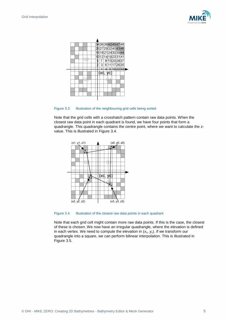
Figure 3.3 Illustration of the neighbouring grid cells being sorted

Note that the grid cells with a crosshatch pattern contain raw data points. When the

closest raw data point in each quadrant is found, we have four points that form a

quadrangle. This quadrangle contains the centre point, where we want to calculate the z-

value. This is illustrated in Figure 3.4.

Figure 3.4 Illustration of the closest raw data points in each quadrant

Note that each grid cell might contain more raw data points. If this is the case, the closest

of these is chosen. We now have an irregular quadrangle, where the elevation is defined

in each vertex. We need to compute the elevation in (xc, yc). If we transform our

quadrangle into a square, we can perform bilinear interpolation. This is illustrated in

Figure 3.5.

Grid Interpolation


Figure 3.5 Illustration of bilinear interpolation

First the interpolation requires the transformation from quadrangle to a normalised

square. This is done in the by computing 8 coefficients in the following way:

30122

30121

032

031

012

011

02

01

yyyyD

xxxxD

yyC

xxC

yyB

xxB

yA

xA

(3.1)

Mapping the coordinates (xc, yc) to the normalised square (dx, dy) is done by solving

Equation (3.2).

02 cbxax (3.2)

Where the coefficients are

122112

1221211212

1221

ACACyCxCc

BCBCADADyDxDb

BDBDa

cc

cc

(3.3)

Solving Equation (3.2) gives us dx

a

acbbdx

2

42 (3.4)

Where is used to choose the correct root. dy can now be computed in two

ways:

0 dx 1

Grid Interpolation


dxDC

dxBAxdy c

11

11

(3.5)

or

dxDC

dxBAxdy c

22

22

(3.6)

Choosing between Equations (3.5) and (3.6) is done in such a way that division by zero is

avoided. (xc, yc) has been mapped to (dx, dy). The task was to compute the elevation in

the point (xc, yc) and this is done in the following way using regular bilinear interpolation:

0132 1111 zdxdyzdydxzdydxzdydxzc (3.7)

If less than four points are found (if one or more quadrants are empty), the double linear

interpolation is replaced with inverse distance weighted interpolation. This is done

according to the following scheme:

22

1

cici

i

yyxxw

(3.8)

N

i

is ww1

(3.9)

N

i

ii

s

c zww

z1

1 (3.10)

The method works fairly efficiently, but it has one drawback. The quadrant search is

heavily dependent on the orientation of the bathymetry. If the bathymetry is rotated 45

degrees 4 completely different points might be used for the interpolation. For this reason

there is also a Triangular interpolation method, which can be used, and this method

should be direction independent.

3.3.2 Triangular interpolation As mentioned previously the ‘Bilinear Interpolation’ is dependent on the orientation of the

bathymetry. The ‘Triangular Interpolation’ is made as an answer to this problem. First the

closest point to (xc, yc) is found, cf. Figure 3.6.

Grid Interpolation


Figure 3.6 Illustration of triangular interpolation

In this example the point (x0, y0, z0) is the closest point. When this point is identified, two

quadrants are identified – indicated by the light grey and the dark grey areas. The closest

points in these two quadrants are then found. They can be seen on the figure as (x1, y1,

z1) and (x2, y2, z2). The interpolation is then done in two steps.

First the coefficients describing the plane defined by the 3 found points are computed:

000

01020201

01020201

01020201

01020201

ByAxzC

yyxxyyxx

zzxxzzxxB

yyxxyyxx

zzyyzzyyA

(3.11)

And secondly, the actual interpolation is done:

CByAxz ccc (3.12)

If less than 3 points are found, inverse distance weighted interpolation is used. The

triangular interpolation is more time consuming due to the more complex direction

independent search, but better end results should be achieved with this method.

3.3.3 Inverse distance weighted interpolation

The ‘Inverse Distance Weighted Interpolation’ is based on the scheme described in

Equations (3.8) - (3.10).

Please note that the quadrant search is heavily dependent on the orientation of the

bathymetry. Thus, if the bathymetry is rotated 45 degrees four completely different points

may be used for the interpolation.

Grid Interpolation


3.3.4 Inverse squared distances weighted interpolation

The ‘Inverse Squared Distance Weighted Interpolation’ is based on the ‘Inverse Distance

Weighted Interpolation’ but using the squared distance points in the search criteria. The

applied scheme is thus defined by:

22

1

cici

iyyxx

w

(3.13)

N

i

is ww1

(3.14)

N

i

ii

s

c zww

z1

1 (3.15)

Please note that the quadrant search is heavily dependent on the orientation of the

bathymetry. Thus, if the bathymetry is rotated 45 degrees four completely different points

may be used for the interpolation.

Mesh Generation


4 Mesh Generation

The mesh generator can construct meshes that consist of both triangular and

quadrangular elements. The approach being that the area of interest is divided up into

regions described through polygons. Each polygon may have a triangular or a

quadrangular mesh generated within. The complementary area is by default populated

with a triangular mesh.

The steps to generate such a mesh are the following:

• Define polygons to be used for quadrangular mesh

• Set properties for each (default values used if local properties are not supplied)

• Generate the mesh within each polygon

• Use the triangular mesh approach for the area not contained within any of the

polygons.

Thus the overall idea is to generate the quadrangular mesh first and then to use the

triangular mesh to patch the mesh together.

4.1 Triangular Mesh Generation

The generation of triangles is based on the ‘Triangle’ code, developed by Jonathan

Shewchuk /1/.

Additional information regarding the functionality can be found on the web page

http://www.cs.cmu.edu/~quake/triangle.html.

4.2 Quadrangular Mesh Generation

The quadrangular grid generation may be carried out using two different routines:

• A simple algebraic method using a boxing technique

• An algebraic grid generator using transfinite interpolation

The first of these is robust but may generate skewed grids. The second is efficient but

may not always be successful.

4.2.1 Algebraic box method

The aim is to generate a mesh for a polygon which aligns itself with the polylines that

make up the polygon. The main idea is to break any closed polygon into quadrangles.

Below is a polygon consisting of two polylines l1 and l2 with a number of vertices. The

number of vertices on each polyline may be unequal in general. The polylines are joined

by two arcs. These end arcs consist each of only one line segment. The polygon is

considered as an abstraction of a stream tube i.e. the flow direction is in the direction of

http://www.cs.cmu.edu/~quake/triangle.html

Mesh Generation


the two polylines and the end arcs are transversal to the flow direction. Ideally the end

arcs should be chosen so that these are perpendicular to the flow direction.

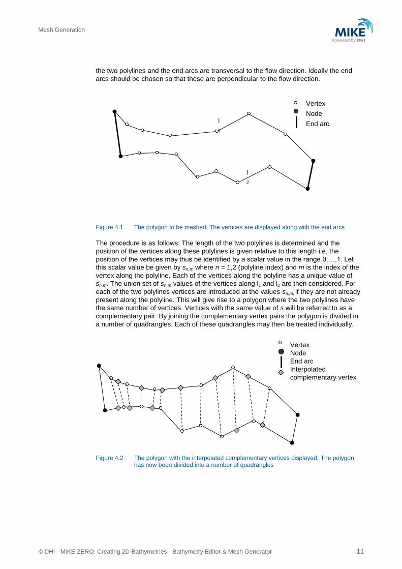
Figure 4.1 The polygon to be meshed. The vertices are displayed along with the end arcs

The procedure is as follows: The length of the two polylines is determined and the

position of the vertices along these polylines is given relative to this length i.e. the

position of the vertices may thus be identified by a scalar value in the range 0,…,1. Let

this scalar value be given by sn,m where n = 1,2 (polyline index) and m is the index of the

vertex along the polyline. Each of the vertices along the polyline has a unique value of

sn,m. The union set of sn,m values of the vertices along l1 and l2 are then considered. For

each of the two polylines vertices are introduced at the values sn,m, if they are not already

present along the polyline. This will give rise to a polygon where the two polylines have

the same number of vertices. Vertices with the same value of s will be referred to as a

complementary pair. By joining the complementary vertex pairs the polygon is divided in

a number of quadrangles. Each of these quadrangles may then be treated individually.

Figure 4.2 The polygon with the interpolated complementary vertices displayed. The polygon

has now been divided into a number of quadrangles

l

1

l

2

Vertex

Node

End arc

Vertex

Node

End arc

Interpolated

complementary vertex

Mesh Generation


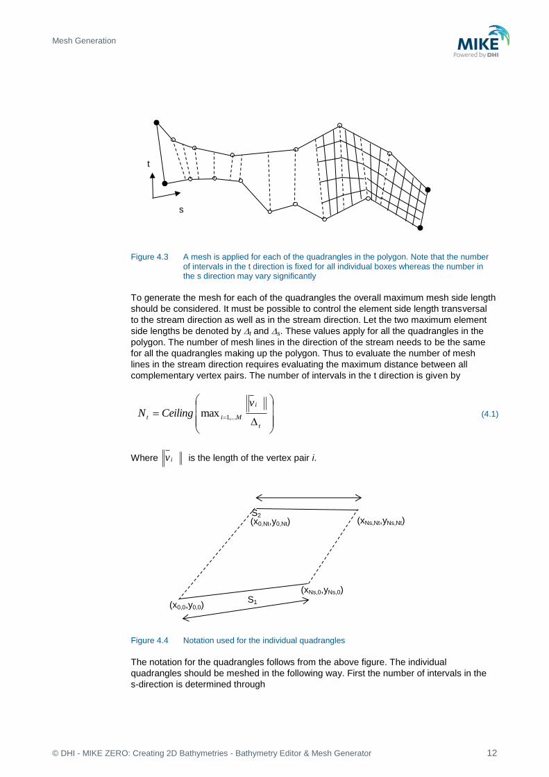
Figure 4.3 A mesh is applied for each of the quadrangles in the polygon. Note that the number

of intervals in the t direction is fixed for all individual boxes whereas the number in the s direction may vary significantly

To generate the mesh for each of the quadrangles the overall maximum mesh side length

should be considered. It must be possible to control the element side length transversal

to the stream direction as well as in the stream direction. Let the two maximum element

side lengths be denoted by t and s. These values apply for all the quadrangles in the

polygon. The number of mesh lines in the direction of the stream needs to be the same

for all the quadrangles making up the polygon. Thus to evaluate the number of mesh

lines in the stream direction requires evaluating the maximum distance between all

complementary vertex pairs. The number of intervals in the t direction is given by

t

i

Mit

vCeilingN ,...1max (4.1)

Where iv

is the length of the vertex pair i.

Figure 4.4 Notation used for the individual quadrangles

The notation for the quadrangles follows from the above figure. The individual

quadrangles should be meshed in the following way. First the number of intervals in the

s-direction is determined through

s

t

(x0,0,y0,0)

(xNs,0,yNs,0)

(xNs,Nt,yNs,Nt) (x0,Nt,y0,Nt)

S1

S2

Mesh Generation


s

s

ssCeilingN

),max( 21 (4.2)

Where

(4.3)

Once the number intervals is known the node locations may be found through

tst

s

tst

s

NN

ts

N

st

N

tsts

ji

NN

ts

N

st

N

tsts

ji

yN

j

N

iy

N

i

N

j

yN

j

N

iy

N

j

N

iy

xN

j

N

ix

N

i

N

j

xN

j

N

ix

N

j

N

ix

,,0

0,0,0,

,,0

0,0,0,

1

111

1

111

(4.4)

Where

ts NjandNi ,,0,,0 (4.5)

Problematic sections may arise for some polygons. Such a polygon is displayed below.

Figure 4.5 A problematic polygon

Problematic sections may be identified as sections with opposing sides having a scalar

product which is non-positive. Using the notation from the earlier figure the criteria is

expressed as

),(),( 0,00,00,0,1 yxyxs NsNs

),(),( ,0,0,,2 NtNtNtNsNtNs yxyxs

Mesh Generation


0,0,

,0,

0,0,

0,0,

NtNtNs

NtNtNs

oNs

oNs

yy

xx

yy

xx (4.6)

4.2.2 Transfinite interpolation

The second option uses a so-called transfinite interpolation to determine the grid points.

The formula uses relative coordinates along the four polylines making up the polygon to

be meshed.

Figure 4.6 The notation used for the transfinite interpolation grid generation

and vary between 0 to 1 along the arcs. The intersection of the boundaries are

identified The intersection of the ‘South’ and the ‘West’ boundary corresponds to

(

he intersections are identified by:

Intersecting boundaries (ξ, η)

‘South’ and ‘West’ (0,0)

‘West’ and ‘North’ (0,1)

‘North’ and ‘East’ (1,1)

‘East’ and ‘South’ (1,0)

‘South’

‘North’

‘West’

‘East’

Mesh Generation


The grid is defined through the expressions

1,11,01

0,110,011

1,0,1,1,01,

1,11,01

0,110,011

1,0,1,1,01,

yy

yy

yyyyy

xx

xx

xxxxx

(4.7)

The expression requires that the four polylines making up the polygon have been

parameterised using the parameters and respectively. These parameters are simply

the distances along the arcs relative to the full length of the polylines.

The distribution of the grid points along the polylines

The grid points along the polylines must obey the location of the original vertices. Thus

the concept of vertex pairs for opposing polylines should be used. Though note that the

vertex pairs no-longer by default are connected by a straight line due to the piecewise

linear nature of the end arcs.

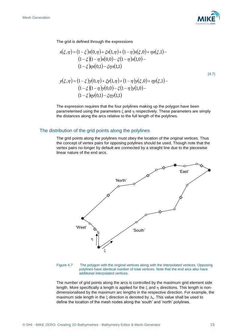
Figure 4.7 The polygon with the original vertices along with the interpolated vertices. Opposing

polylines have identical number of total vertices. Note that the end arcs also have additional interpolated vertices.

The number of grid points along the arcs is controlled by the maximum grid element side

length. More specifically a length is applied for the and directions. This length is non-

dimensionalised by the maximum arc lengths in the respective direction. For example, the

maximum side length in the direction is denoted by s. This value shall be used to

define the location of the mesh nodes along the ‘south’ and ‘north’ polylines.

‘South’

‘North’

‘West’

‘East’

Mesh Generation


The maximum length of the ‘south’ and ‘north’ polylines is used to define the non-

dimensional mesh element side length . Let the two lengths be denoted by lsouth and

lnorth. The non-dimensional maximum side length is defined by

s

northsouth ll

),max(

(4.8)

This value must be satisfied for all line segments along the ‘south’ and ‘north’ polylines.

The approach is to determine the number of intervals for the line segment i through

1,

iii CeilingN (4.9)

Where i corresponds to the i’th vertex.

The procedure for the ‘west’ and ‘east’ arcs follows along the same lines.

4.3 Generating Combined Mesh

The present section outlines the approach that will be adopted for merging the

quadrangular mesh polygons with the surrounding triangular mesh.

The triangular mesh generator has the flexibility to insert so-called Steiner points. Steiner

points are additional vertices used to subdivide line segments into several line segments.

Steiner points are necessary to allow the segments to exist in the mesh while maintaining

the required properties of the mesh such as constraints on the minimum angle and

maximum triangle area.

Figure 4.8 A polygon that has been meshed where additional Steiner points have been inserted

The above figure illustrates the concept of Steiner points. Steiner points are useful when

the whole area is meshed using triangles, but do create a problem when the mesh is

mixed. To overcome this problem the triangulisation routine may be used with the

restriction that Steiner points are not inserted. If this is used on the above case the result

would be along the lines as illustrated in Figure 4.9.

Steiner points

Mesh Generation


Figure 4.9 A triangulisation with the restriction that Steiner points are not allowed

It is especially important that the mesh routine does not insert Steiner points along arcs

which form part of a polygon designated for a quadrangular mesh. To overcome this

problem the idea is to run the triangulisation twice. The first triangulisation is done to

determine the location of Steiner points along arcs without constraints (i.e. arcs not part

of a polygon for quadrangulisation).

Once the Steiner points have been identified along these ‘free’ arcs the Steiner points are

internally converted to vertices. The second tringulisation is then done with the constraint

that Steiner points are not allowed.

The procedure is outlined on the following pages.

Step 1:

Generate the quadrangular mesh.

Step 2:

Insert vertices along the mesh points at

the arcs used for quadrangular mesh.

Mesh Generation


Step 3:

Mark all polygons used for a

quadrangular mesh internally as not

included in the mesh. Then mesh the

remaining area.

Step 4:

Convert all mesh points along ‘free’ arcs

to vertices. Notice the Steiner point at

the north arc of the quadrangular mesh

polygon.

Step 5:

Remove the triangular mesh.

Step 6:

Regenerate the mesh, but this time do

not allow the triangulation to insert

Steiner points.

Mesh Generation


Step 7:

Reintroduce the mesh for the

quadrangular polygons. Resulting in the

final mesh. Note that the Steiner point

previously introduced at north arc of the

box is no longer present.

4.4 Smoothing the Mesh

After the generation of the mesh it is prudent to smooth the mesh to obtain a better

applicability in a simulation. Smoothing a mesh is the effort to position the nodes in a way

such that the angles in each element and the element area are as large as possible. The

smoothing only affects triangular mesh elements.

Figure 4.10 Definition: Moving node point due to smoothing

The location of the Smoothed point Q' is found through

elementsN

i

ielements

elements

PQNN

Q1

23

1' (4.10)

The smoother may be applied iteratively and will converge to a mesh where the following

holds for each point.

elementsN

i

i

elements

PN

Q1

1' (4.11)

I.e. every point is placed in the centre of mass of the surrounding polygon.

Please note that though the system is converging towards a unique solution this may not

be a solution which satisfies the mesh constraints as set up in the Mesh Generation

menu (plus local polygons if they exist). The idea is to do the mesh smoothing one step at

Mesh Generation


a time and then evaluate the mesh and reset any nodes which give rise to elements

which do not satisfy the constraints.

The measure consists of the element area and the smallest angle in the element. If one

of these is smaller than the allowed values then the calculated measure evaluates to

false.

Two options can be included when smoothing the mesh:

• Smoothing constrained by mesh criterion

If this is not selected the measure will always evaluate to true

• Leave mesh nodes at arcs untouched

If this is not selected ALL internal nodes may be relocated. Otherwise, if a node

originally was part of a defined arc or is a single user defined node then the node is

not allowed to be moved during the smoothing.

4.5 Refinement by Bisection

A mesh may be refined by subdividing the faces of the existing elements. The bisection

method is designed to only change the size of the elements in a given mesh without

changing the overall quality of the mesh i.e. the angles of the refined mesh will not

become less than the original mesh.

The mesh bisection method follows some clear principles:

Take all elements faces of the original mesh and place a node at the mid points (hence

bisection). Consider each element in the original mesh. Depending on whether the

element is triangular or quadrilateral the approach varies slightly.

For a triangular element the approach is as illustrated in Figure 4.11.

Figure 4.11 Bisection of triangular element

As can be seen from Figure 4.11, the operation will give rise to 4 new elements per

triangular element in the original mesh and 3 new element faces.

For a quadrilateral element the approach is as illustrated in Figure 4.12.

Mesh Generation


Figure 4.12 Bisection of quadrangular element

As can be seen from Figure 4.12 also for the quadrangular elements the process

introduces 4 new elements per quadrangular element in the original mesh and 4 element

faces. Note that the quadrangular elements also generate an additional mesh node on

top of the ones caused by the face bisection.

The refinement may in principle be applied an arbitrary number of times. The table below

summarises the number of topological elements (faces, elements, nodes) as a function of

the number of refinements (n).

Number of

topological

elements

Original mesh 1st

refinement 2nd

refinement n’th refinement (2n)

Faces F 2F+3T+4Q 4F+18T+24Q 2𝑛𝐹 + (3𝑇 + 4𝑄) ∑ 2𝑖−1

𝑛

𝑖=1

4𝑛−𝑖

Triangular

elements

T 4T 16T 4𝑛𝑇

Quadrangular

elements

Q 4Q 16Q 4𝑛𝑄

Nodes N N+F+Q N+3F+3T+9Q 𝑁 + 𝐹 ∑ 2𝑖

𝑛−1

𝑖=0

+ 𝑄 ∑ 4𝑖

𝑛−1

𝑖=0

+(3𝑇 + 4𝑄) ∑ (∑ 2𝑖−1

𝑗

𝑖=1

4𝑗−𝑖)

𝑛−1

𝑗=1

Mesh Interpolation


5 Mesh Interpolation

The Mesh Generator gives two possibilities with respect to interpolation for triangular

elements. The two possible interpolation routines are

• Natural neighbour

• Linear interpolation

These interpolation methods are valid independent of the type of mesh used. The

interpolation requires values only at the mesh nodes and will base the interpolation solely

on the scatter data. Thus whether the nodes are part of a triangular or quadrangular

mesh is of no significance. These methods may however not be the correct ones to use

for river beds or other water ways in an in land setting. In particular the interpolated

surface generated for a strongly meandering river may give rise to a highly erroneous

river bed (see Figure 5.1).

Figure 5.1 A meandering river with a point (O) at which the topography is to be interpolated

using the natural neighbour method. The crosses indicate location at which data is located. The grey polygon illustrates the weights of the values at A-E

As can be seen from the above figure, the point B will have a significant weight and thus

impact on the interpolated value at O. Point B is located on the opposite bank of the

interpolation location O and thus the bed level may be very different from the true value at

O. One would assume that the actual level at O is closer to the values at A and C in the

stream direction. Further the interpolation routine also takes the values at D and E into

account even though the points are located outside the main river.

To create sound interpolated topographies in river beds an interpolation routine that

emphasises values in the stream direction and does not interpolate across riverbanks has

been developed for quadrangular elements.

A B

D

E

C

Mesh Interpolation


5.1 Interpolation Accommodating the Stream Direction

To accommodate higher weights on points positioned in the stream direction a modified

version of the inverse distance method is applied. The inverse distance is a simple

interpolation routine. A neighbourhood about the interpolated point is identified and a

weighted average is taken of the observation values within this neighbourhood. The

weights are a decreasing function of distance ri and are typically given by

p

i

N

i

p

ii

rrw

111

1

(5.1)

for point i where p is greater than 0.

The distance r is often given by the Pythagorean distance but may be any measure. The

latter may be utilised to accommodate the weighting of points in the stream direction. The

coordinate system will be constructed so that at the mesh nodes the coordinates take on

integer values. At intermediate locations the coordinates are found through bilinear

interpolation. The river segment or polygon when pictured in the mesh based coordinate

system is simply a rectangular as illustrated in Figure 5.2.

Figure 5.2 The meandering river on the left without the mesh displayed. The right figure

illustrates the river overlaid with the mesh

Figure 5.3 The polygon displayed in the mesh coordinate system (j,k)

In the new coordinate system the points A, B and C will have the following coordinates:

A: (jA,kA)

B: (jB,kB)

C: (jC,kC)

where j and k may take on non-integer values.

A B

D

E

C

A B

D

E

C

C

B

A j

k

Mesh Interpolation


The location at which the interpolation is to take place has coordinates (jo,ko). The z-value

at O may then be expressed as

CBA q

Oi

p

Oi

i

CBA q

Oi

p

Oi

O

kkjj

z

kkjjz

,,

1

,,

1 (5.2)

where q > p. The latter is to ensure that the effect of the j coordinate decays more slowly

than the effect of the k-coordinate. Both p and q should be user defined (advanced

option). Some experimentation is needed to identify proper default values of p and q.

The bilinear interpolation to be used for determining the (j,k) coordinates for scatter points

not placed at a mesh node is found through

Figure 5.4 A mesh element with four nodes with mesh coordinates (j,k), (j+1,k),(j,k+1) and

(j+1,k+1). The mesh coordinates of (x,y) are sought

The coordinates of (x,y) satisfy the following equation

0010

0010

00

00

0111

0111

01

01

0010

0010

00

00

yy

xxs

y

x

yy

xxs

y

xt

yy

xxs

y

x

y

x

(5.3)

Where s,t lies within the interval [0;1]. This equation may be re-arranged as

11011000

11011000

0001

0001

0010

0010

00

00

yyyy

xxxxst

yy

xxt

yy

xxs

yy

xx

(5.4)

which in turn may be expressed as

2

1

2

1

2

1

2

1

c

cst

b

bt

a

as

d

d (5.5)

(x00,y00)

(x10,y10)

(x11,y11) (x01,y01)

(x,y)

Mesh Interpolation


This equation may be rewritten as a set of two equations

11

11

211212212112

2

2112 0)(

scb

sadt

dbdbscdcdbabascaca

(5.6)

of which the first is second order algebraic equation in s. Once the two solutions are

found t may be determined from equation number. The true solution is the one that gives

rise to a set of s and t lying within the interval 0 to 1.

The mesh coordinates of the point (x,y) are thus given by (j+s,k+t).

5.2 Interpolation using Prioritisation of Scatter Data

The prioritisation is carried out by applying weights to the individual scatter data sets.

These weights may be assigned globally and locally.

The methodology used for prioritisation during interpolation is the following:

Assume n sources of data each being supplied in any of the accepted data formats (xyz,

dfs2, dfsu, mesh). Let these data sets be denoted by D1 , D2 …, Dn.

• The interpolation is done separately for each data source Di. Hereby there will be a

mesh Mi with values only dependent on data source Di.

• Each data source has an associated weight wi in the range 0 to 1.

• The resulting mesh is obtained through the sum

𝑀 = ∑ 𝑀𝑖𝑤𝑖

𝑛

𝑖=1

(5.7)

Where the weights satisfy

∑ 𝑤𝑖 = 1

𝑛

𝑖=1

(5.8)

• The concept is also used with localised weights associated with user specified

regions.

The process is illustrated below using a set-up with three different data sources.

Mesh Interpolation


Figure 5.5 Mesh point P in setup with three different data sources. Each scatter data source has

associated weight

After interpolation, the mesh point P will have a z value based on the three interpolations

from data source 1 to 3 weighted according to the weights:

𝑍(𝑃) = 𝑤1𝑍(𝑃, 𝐷1) + 𝑤2𝑍(𝑃, 𝐷2) + 𝑤3𝑍(𝑃, 𝐷3) (5.9)

Where Z(P,Di) is the result of an interpolation only including data source Di.

To apply local weights prioritisation polygons must be defined. Prioritisation polygons are

user defined areas where a specific set of prioritisation weights are to be used.

Prioritisation polygons are different from the polygons used for specifying mesh

resolutions and mesh type.

Mesh Analysis and Editing


6 Mesh Analysis and Editing

During the process of creating the mesh it is possible to analyse the mesh for its

applicability in a simulation and to edit local mesh elements.

6.1 Mesh Analysis

It is possible to analyse a mesh for its applicability in a simulation by evaluating the

restricting time step for each mesh element.

The analyses of a mesh consists of considering

• The element area

• The smallest angle within each element

• The CFL stability criteria

Figure 6.1 Definition of node point and position in mesh analysis

The area of a triangular element is given by

131213122

1xxyyyyxxA (6.1)

The area of a quadrilateral is calculated as the sum of areas of the two triangles that

matches the quadrilateral.

The smallest angle may be evaluated by calculating the normalised scalar product:

210

2

10

2

12

2

12

101210121yyxxyyxx

yyyyxxxxs

(6.2)

The quantity S varies between 0 and 2 where 0 refers to the smallest angle and 2 the

largest.

The time step Δt evaluated on basis of the CFL number is given by

gh

facelengthCFLt

2

min (6.3)

Mesh Analysis and Editing


where h is water depth (water level - topography) and g is 9.82 m2/s.

6.2 Collapsing Elements

Effectively the mesh element (triangular or quadrangular) is collapsed by taking all nodes

in the mesh and collapsing them to the centre point of the element (centre of mass). Note

that the procedure may remove up to four mesh elements.

The collapse of an element may be achieved by subsequent collapses of cells faces and

a final move of the node to the centre of mass of the original mesh element. The process

is illustrated in Figure 6.2 for a triangular element. The procedure for the quadrangular

element requires four face collapses instead of three.

Figure 6.2 Process for collapsing triangular element

The z value at the new node is obtained through interpolation based on the user settings.

The code value of the mesh node is set to the maximum of the nodes of the collapsed

element. The data used as scatter data for the interpolation are the values at the mesh

nodes.

Shoreline Files


7 Shoreline Files

The shoreline files are a collection of different files especially formatted for use in the

Shoreline Morphology model, which can be applied from within ST in MIKE 21 Coupled

Model FM.

7.1 Baseline

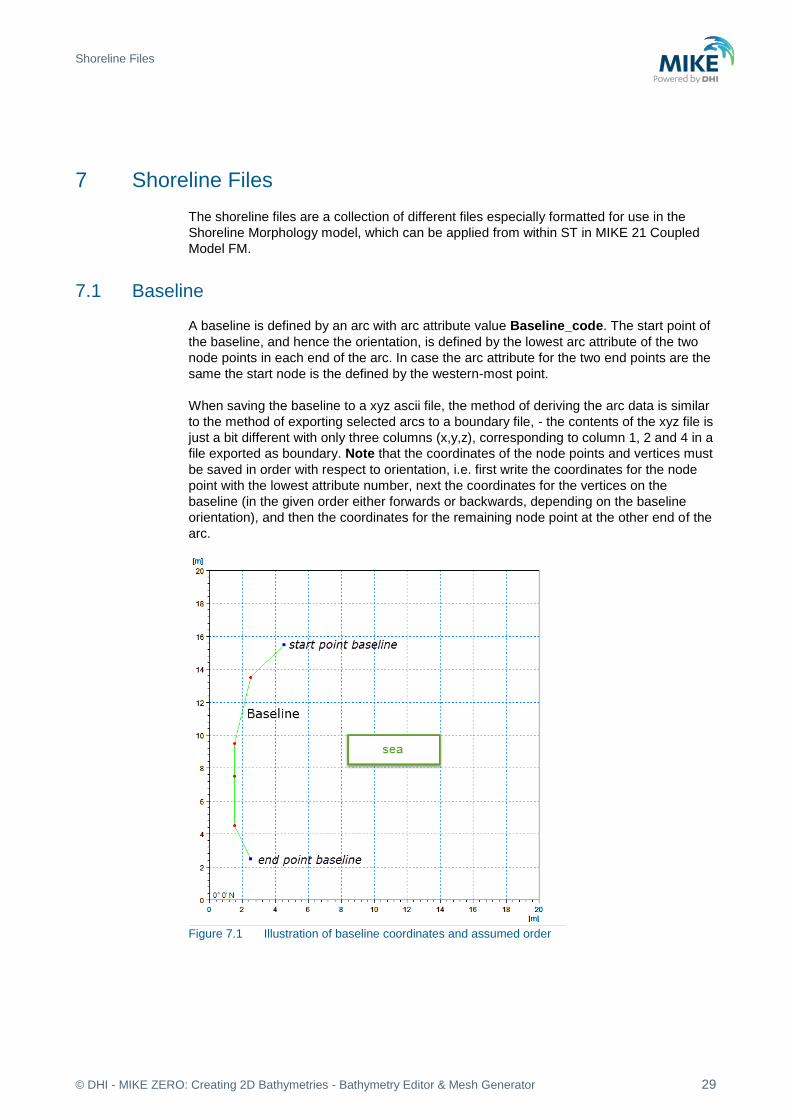
A baseline is defined by an arc with arc attribute value Baseline_code. The start point of

the baseline, and hence the orientation, is defined by the lowest arc attribute of the two

node points in each end of the arc. In case the arc attribute for the two end points are the

same the start node is the defined by the western-most point.

When saving the baseline to a xyz ascii file, the method of deriving the arc data is similar

to the method of exporting selected arcs to a boundary file, - the contents of the xyz file is

just a bit different with only three columns (x,y,z), corresponding to column 1, 2 and 4 in a

file exported as boundary. Note that the coordinates of the node points and vertices must

be saved in order with respect to orientation, i.e. first write the coordinates for the node

point with the lowest attribute number, next the coordinates for the vertices on the

baseline (in the given order either forwards or backwards, depending on the baseline

orientation), and then the coordinates for the remaining node point at the other end of the

arc.

Figure 7.1 Illustration of baseline coordinates and assumed order

Shoreline Files


Example of output file (Baseline.xyz):

4.5 15.5 0 (point id 7, attribute 100 - last point in arc, first point on baseline)

2.5 13.5 0 (point id 4)

1.5 9.5 0 (point id 2)

1.5 7.5 0 (point id 1)

1.5 4.5 0 (point id 0)

2.5 2.5 0 (point id 3, attribute 101 - first point in arc, last point on baseline)

7.2 Coastline

A coastline is defined by an arc with arc attribute value Coastline_code. The start point

of the coastline is defined by the lowest arc attribute of the two node points in each end of

the arc. In case the arc attribute for the two end points are the same the start node is the

defined by the western-most point.

The coastline arc can initially be defined by any number of points, however in order to

match the baseline the number of points on the coastline needs to be +1 compared to the

number of points on the baseline, and the position of the coastline points should be

located at the centre of the baseline sections when projected perpendicular to the

baseline.

Figure 7.2 Coastline arc before modifying the position of vertices to be positioned at centre of

baseline sections

Shoreline Files


Example: contents in mdf-file before coastline modification: [POINTS]

Data = '13 0 1.5 4.5 0 0 0 1 1.5 7.5 0 0 0 2 1.5 9.5 0 0 0 3 2.5

2.5 101 0 1 4 2.5 13.5 0 0 0 5 4.5 5.5 0 0 0 6 4.5 9.5 0 0 0 7 4.5 15.5

100 0 1 8 5.5 1.5 0 111 1 9 5.5 2.5 0 0 0 10 5.5 3.5 0 0 0 11 6.5 11.5 0

0 0 12 7.5 15.5 0 110 1'

EndSect // POINTS

[ARCS]

Data = '2 0 8 12 5 9 10 5 6 11 110 1 3 7 4 0 1 2 4 100'

EndSect // ARCS [ARCS]

The method of modifying the coastline points to match the baseline is described in the

following.

1. An array holding the position of the coastline points (in order) is defined

2. For each baseline section the following is done:

a. the centre point position (x,y) is located

b. the line that starts in (x,y) and is perpendicular to the baseline section is

defined:

Shoreline Files


c. A new coastline point (xc,yc) is found at the position where the original coastline

arc intersects with the perpendicular line from the baseline:

3. Finally, a new coastline is created using the first and last node point in the initial

coastline file and the updated coastline points.

Shoreline Files


Example: contents in mdf-file after coastline modification: [POINTS]

Data = '13 0 1.5 4.5 0 0 0 1 1.5 7.5 0 0 0 2 1.5 9.5 0 0 0 3 2.5

2.5 101 0 1 4 2.5 13.5 0 0 0 5 4.5 15.5 100 0 1 6 4.5009074410163334

6.4609800362976406 0 0 0 7 4.5009074410163334 8.6025408348457351 0 0 0 8

4.7549909255898362 5.0090744101633389 0 0 0 9 5.5 1.5 0 111 1 10

5.7350272232304897 10.816696914700545 0 0 0 11 6.5698729582577133

11.869328493647913 0 0 0 12 7.5 15.5 0 110 1' EndSect // POINTS

[ARCS]

Data = '2 0 9 12 5 8 6 7 10 11 110 1 3 5 4 0 1 2 4 100'

EndSect // ARCS

When saving the coastline to a xyz ascii file, the method of deriving the arc data is similar

to the method of exporting selected arcs to a boundary file, - the contents of the xyz file is

just a bit different with only three columns (x,y,z), corresponding to column 1, 2 and 4 in a

file exported as boundary (z-value can be set to 0). Note that the coordinates of the node

points and vertices are saved in order with respect to orientation, i.e. first the coordinates

for the node point with the lowest attribute number are written, next the coordinates for

the vertices on the modified coastline (in the given order either forwards or backwards,

depending on the baseline orientation), and finally, the coordinates for the remaining

node point at the other end of the arc.

Example of output file (Coastline.xyz):

7.5 15.5 0 (new point id 12, attribute 110 - last point in arc, first point on coastline)

6.5698729582577133 11.869328493647913 0

5.7350272232304897 10.816696914700545 0

4.5009074410163334 8.6025408348457351 0

4.5009074410163334 6.4609800362976406 0

4.7549909255898362 5.0090744101633389 0

5.5 1.5 0 (new point id 9, attribute 111 - first point in arc, last point on baseline)

Shoreline Files


7.3 Edge Map

The edge map defines which coastline edge/section each element in the mesh belongs

to. The edge map is defined in an area limited by the baseline and an arc forming a

limiting edge map line in a variable distance from the baseline as shown below. The edge

map values are saved in a dfsu file, which are based on the generated (or loaded) mesh.

The creation of an edge map thus requires a mesh, a baseline and an edge map line.

An edge map line is defined by an arc with arc attribute value Edge_map_code. The

edge map arc can be defined by any number of points and is used to from an outer limit

of the edge map. Along with the baseline and leading lines, extending from the baseline

points and perpendicular to the local baseline orientation, the edge map line forms

polygons that defines which section the individual elements in the mesh belong to.

The mesh elements, whose centre position is located within an edge map polygon, are

allocated the integer value that corresponds to the coastline section (i.e. baseline section

number + 1).

Shoreline Files


Example: contents in mdf-file containing mesh, baseline arc and edge map arc: [POINTS]

Data = '10 0 1.5 4.5 0 0 0 1 1.5 7.5 0 0 0 2 1.5 9.5 0 0 0 3 2.5

2.5 0 101 1 4 2.5 13.5 0 0 0 5 4.5 15.5 0 100 1 6 6.9755469755469752

6.1776061776061777 0 0 0 7 8.416988416988417 1.3127413127413128 0 0 1 8

9.4465894465894458 12.818532818532818 0 0 0 9 9.6782496782496779

16.653796653796654 0 0 1'

EndSect // POINTS

[ARCS]

Data = '2 0 3 5 4 0 1 2 4 100 1 9 7 2 8 6 120'

EndSect // ARCS

…

[MESH]

Node_Count = 1109

Max_Node_Count = 500000

Element_Count = 2087

Max_Element_Count = 500000

Segment_Count = 0

Max_Segment_Count = 500000

Tri_Point_Count = 1109

Tri_Element_Count = 2087

Nodes_1 = '0 0.55045871559633031 0.40366972477064222

4.9775168444853195 1 1 0.66055045871559637 17.944954128440369

4.9734124177676513 1 2 15.963302752293577 0.25688073394495414 -

9.9914120028450721 1 3 15.963302752293577 17.98165137614679 -

9.9156919720941712 1 4 0.61034224253743041 9.9451116840525913

4.9959048897791174 …

…

10.487354704113843 4.5178970049871126 0 1108 0.95410172040716057

6.4192123372189789 4.995163126330171 0 '

Elements_1 = '3 0 78 283 287 0 -1 3 1 710 19 709 0 -1 3 2 590 192

589 0 -1 3 3 733 729 175 0 -1 3 4 894 370 100 0 -1 3 5 25 1077 1036 0 -1

3 6 745 176 743 0 -1 3 7 839 694 115 0 -1 3 8 77 840 836 0 -1 3 9 237 239

35 0 -1 3 10 752 723 184 0 -1 3 11 719 739 718 0 -1 3 12 825 826 610 0 -1

3 13 256 835 823 0 -1 3 14 787 788 226 0 -1 3 15 435 537 542 0 -1 3 16

325 82 422 0 -1 3 17 578 579 152 0 -1 3 18 521 427 522 0 -1 3 19 409 925

368 0 -1 3 20 103 375 382 0 -1 3 21 923 910 18 0 -1 3 22 868 42 864 0 -1

3 23 707 705 706 …

…

3 2080 477 1105 1021 0 -1 3 2081 505 1106 1036 0 -1 3 2082 675 1106 574 0

-1 3 2083 1107 569 626 0 -1 3 2084 4 1107 1054 0 -1 3 2085 1067 1108 601

0 -1 3 2086 1108 600 1065 0 -1 '

EndSect // MESH

Shoreline Files


The method of creating the edge map is described in the following.

1. An array holding the position of the edge map line arc is defined

2. For each baseline point , i:

a. the leading line that is perpendicular to the averaged baseline orientation is

found

b. the coordinate (x,y) for the point where the leading line intersects with the edge

map line is found

3. For each baseline section a polygon is created based on the two points on the

baseline and the corresponding points where the leading lines cross the edge map

line. The polygons are saved in an array.

4. An array for hold the edge map values in the mesh is defined.

Shoreline Files


5. For each mesh element the centre position is compared with the calculated

polygons.

c. If the element is located within one of the polygons the element value is set to

the integer value corresponding to the baseline section for the given polygon

(e.g. for baseline section located between baseline point 0 and 1, the edge map

value is set to 1).

d. If the element is located outside any polygon the value is set to a delete value.

When Exporting the edge map the values are saved to a dfsu file.

Shoreline Files


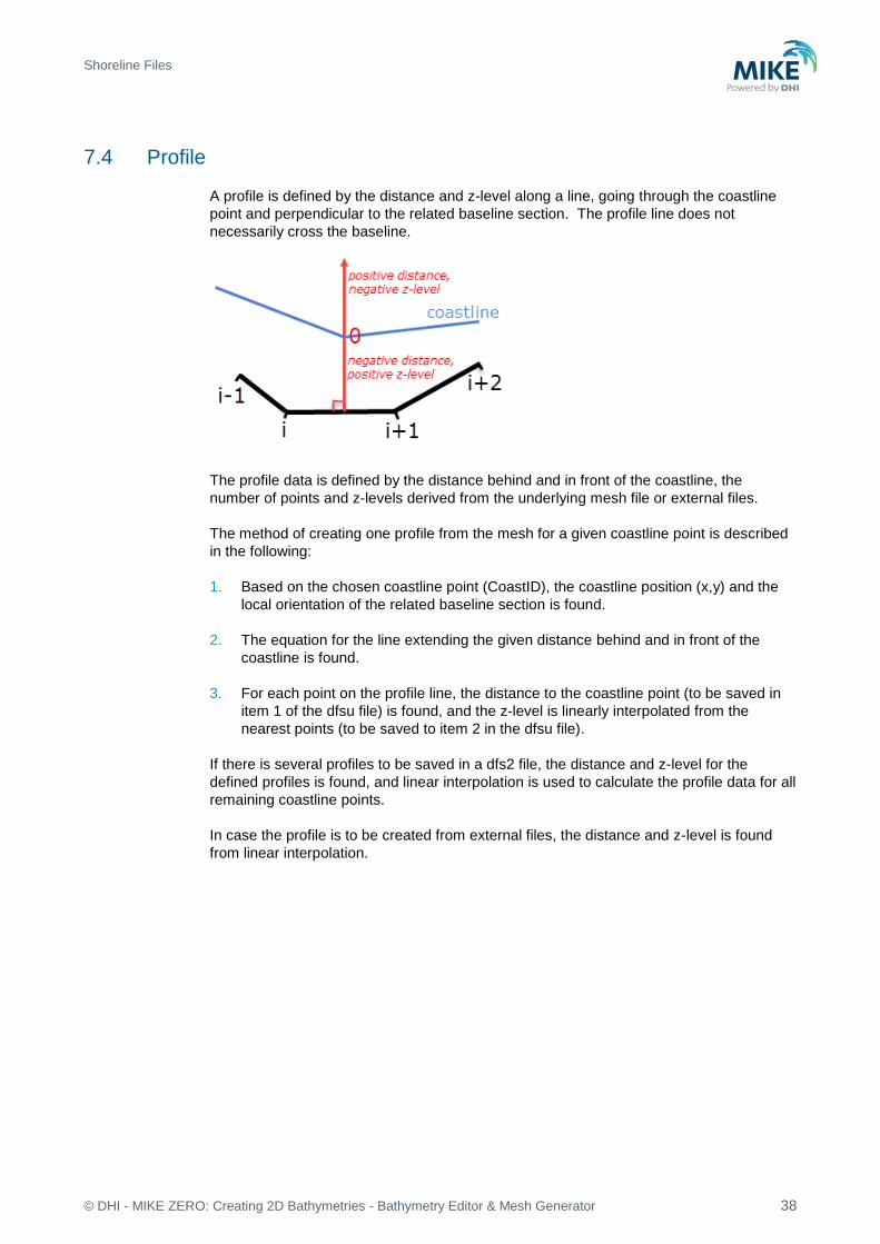
7.4 Profile

A profile is defined by the distance and z-level along a line, going through the coastline

point and perpendicular to the related baseline section. The profile line does not

necessarily cross the baseline.

The profile data is defined by the distance behind and in front of the coastline, the

number of points and z-levels derived from the underlying mesh file or external files.

The method of creating one profile from the mesh for a given coastline point is described

in the following:

1. Based on the chosen coastline point (CoastID), the coastline position (x,y) and the

local orientation of the related baseline section is found.

2. The equation for the line extending the given distance behind and in front of the

coastline is found.

3. For each point on the profile line, the distance to the coastline point (to be saved in

item 1 of the dfsu file) is found, and the z-level is linearly interpolated from the

nearest points (to be saved to item 2 in the dfsu file).

If there is several profiles to be saved in a dfs2 file, the distance and z-level for the

defined profiles is found, and linear interpolation is used to calculate the profile data for all

remaining coastline points.

In case the profile is to be created from external files, the distance and z-level is found

from linear interpolation.

References


8 References

/1/ Jonathan Richard Shewchuk, Triangle: Engineering a 2D Quality Mesh Generator and

Delaunay Triangulator, in ``Applied Computational Geometry: Towards Geometric

Engineering'' (Ming C. Lin and Dinesh Manocha, editors), volume 1148 of Lecture Notes in

Computer Science, pages 203-222, Springer-Verlag, Berlin, May 1996.

Date post:	24-Jun-2020
Category:	Documents
Upload:	others
View:	2 times
Download:	0 times

MIKE ZERO: Creating 2D Bathymetries › 2017 › General › ... · 2016-12-27 · MIKE ZERO:...

Documents