Millimeter-Wave Beamforming: Antenna Array … Beamforming: Antenna Array Design Choices &...

Millimeter-Wave Beamforming: Antenna Array Design Choices & Characterization White Paper

Millimeter-wave bands are of increasing interest for the satellite industry and under discussion as potential

5G spectrum. Antennas for 5G applications make use of the shorter element sizes at high frequencies to

incorporate a larger count of radiating elements. These antenna arrays are essential for beamforming

operations that play an important part in next generation networks.

This white paper introduces some of the fundamental theory behind beamforming antennas. In addition to

these basic concepts, calculation methods for radiation patterns and a number of simulations results, as

well as some real world measurement results for small linear arrays are shown. Due to the bandwidths

likely to be employed in such applications, a non-standard way of graphical representation is proposed.

Note:

Please find the most up-to-date document on our homepage

http://www.rohde-schwarz.com/appnote/1MA276

Whi

te P

aper

M. R

eil,

G. L

loyd

10.2

016 –

1MA

276_

2e

http://www.rohde-schwarz.com/appnote/1MA276

Table of Contents

1MA276_2e Rohde & Schwarz Millimeter-Wave Beamforming: Antenna Array Design Choices & Characterization

2

Table of Contents

1 Introduction ......................................................................................... 1

2 Beamforming Signals ......................................................................... 2

2.1 Phase Coherent Signal Generation............................................................................ 2

2.2 Signal Propagation ...................................................................................................... 3

3 Beamforming Architectures ............................................................... 5

3.1 Analog Beamforming .................................................................................................. 5

3.2 Digital Beamforming .................................................................................................... 7

3.3 Hybrid Beamforming ................................................................................................... 8

4 Linear Array Antenna Theory .......................................................... 10

4.1 Theoretical Background ............................................................................................10

4.2 Design Choices ..........................................................................................................11

4.3 Application Examples ...............................................................................................13

5 Linear Array OTA Measurement ...................................................... 16

5.1 Enhancing the Simulation with Measurement Data ...............................................16

5.1.1 Measurement Results for single Elements ..................................................................16

5.1.2 Simulation Results based on measured single Element Patterns ...............................17

5.2 Antenna Scan .............................................................................................................19

5.3 Further reading ..........................................................................................................20

6 Results and Outlook ......................................................................... 21

7 Appendix ........................................................................................... 22

7.1 MATLAB® Pattern Generation Script .......................................................................22

7.1.1 Main Function ..............................................................................................................22

7.1.2 Linear Array Factor Function .......................................................................................24

8 References ........................................................................................ 25

1 Introduction


1

1 Introduction

Current cellular 4G networks face a multitude of challenges. Soaring demand for mobile

high resolution multimedia applications brings these networks ever closer to their

practical limits.

5G networks are envisioned to ease the burden on the current infrastructure by offering

significantly higher data rates through increased channel bandwidths. Considering the

shortage of available frequencies traditionally used for mobile communications, mm-wave

bands became a suitable alternative. The large bandwidth available at these frequencies

helps to offer data rates that satisfy 5G demands.

However, the mobile environment at these mm-wave bands is far more complex than at

the currently used frequencies. Higher propagation losses that greatly vary depending on

the environment require an updated network infrastructure and new hardware concepts.

Beamforming antenna arrays will play an important role in 5G implementations since

even handsets can accommodate a larger number of antenna elements at mm-wave

frequencies. Aside from a higher directive gain, these antenna types offer complex

beamforming capabilities. This allows to increase the capacity of cellular networks by

improving the signal to interference ratio (SIR) through direct targeting of user groups.

The narrow transmit beams simultaneously lower the amount of interference in the radio

environment and make it possible to maintain sufficient signal power at the receiver

terminal at larger distances in rural areas.

This paper gives an overview of the beamforming technology including signals, antennas

and current transceiver architectures. Furthermore, simulation techniques for antenna

arrays are introduced and compared to actual measurement results taken on a small

array. The theoretical antenna simulation results presented herein can be reproduced

using the MATLAB® scripts in Appendix 7.1. All equations presented in this paper apply to

linear antenna arrays, which for the purpose of this paper are defined as an array of

equally spaced, individually excitable n radiating elements placed along one axis in a

coordinate system, following [1].

2 Beamforming Signals


2


Beamforming in general works with simple CW-signals as well as with complex

modulated waveforms. Candidate waveforms for 5G are a current research topic, since

many of today’s implementations suffer great disadvantages at millimeter wave bands [2].

This chapter will first introduce phase coherent signal generation before giving an

overview of the most important propagation characteristics of these signals.

2.1 Phase Coherent Signal Generation

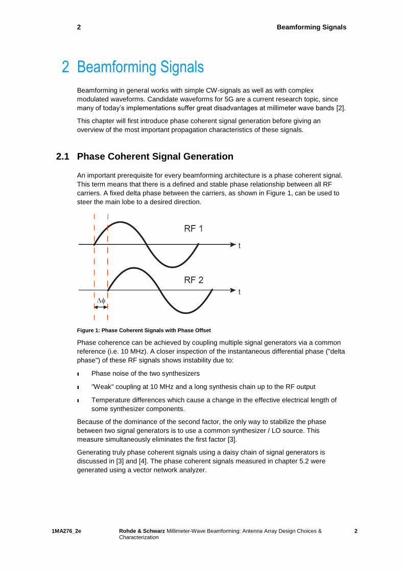
An important prerequisite for every beamforming architecture is a phase coherent signal.

This term means that there is a defined and stable phase relationship between all RF

carriers. A fixed delta phase between the carriers, as shown in Figure 1, can be used to

steer the main lobe to a desired direction.

Figure 1: Phase Coherent Signals with Phase Offset

Phase coherence can be achieved by coupling multiple signal generators via a common

reference (i.e. 10 MHz). A closer inspection of the instantaneous differential phase ("delta

phase") of these RF signals shows instability due to:

ı Phase noise of the two synthesizers

ı "Weak" coupling at 10 MHz and a long synthesis chain up to the RF output

ı Temperature differences which cause a change in the effective electrical length of

some synthesizer components.

Because of the dominance of the second factor, the only way to stabilize the phase

between two signal generators is to use a common synthesizer / LO source. This

measure simultaneously eliminates the first factor [3].

Generating truly phase coherent signals using a daisy chain of signal generators is

discussed in [3] and [4]. The phase coherent signals measured in chapter 5.2 were

generated using a vector network analyzer.



3

2.2 Signal Propagation

All signals radiated from any kind of antenna share the same basic characteristics.

Multipath fading and delay spread significantly reduce the capacity of a cellular network.

Congestion of the available channels and co-channel interference further reduce the

practical network capacity [5].

ı Free Field Attenuation: Electromagnetic waves are attenuated while travelling from

the transmitter to the receiver. The free field attenuation describes the attenuation

which the signal will suffer due to the distance between the two stations.

The Friis formula determines the free field attenuation:

𝑃𝑟,𝑑𝐵 = 𝑃𝑡,𝑑𝐵 + 𝐺𝑡,𝑑𝐵 + 𝐺𝑟,𝑑𝐵 + 20𝑙𝑜𝑔10(𝜆

4𝜋𝑅) (1)

Where 𝑃𝑟,𝑑𝐵 is the received power level in dB, 𝑃𝑡,𝑑𝐵 the transmitted power and

𝐺𝑟,𝑑𝐵 and 𝐺𝑡,𝑑𝐵 the receive and transmit antenna gain in dBi.

Figure 2 (left) illustrates the free field attenuation over a large frequency band.

Even in case of a perfect line of sight (LoS) transmission, there are many different

factors that additionally affect the magnitude of the received signal. As shown in

Figure 2 (right), the resulting overall attenuation varies greatly depending on the

frequency and radiation environment.

Figure 2: Free Field Attenuation approximation according to Friis Equation (left) and Attenuation due to

Atmospheric Gases (right). Source: [6], pp. 16



4

ı Fading: The phase shift in multipath signals is non-constant due to the time variant

nature of the channel. Expression (2) shows the time-dependent received multipath

signal, where the complex values 𝑎𝑛(𝑡) and 𝑒−𝑗𝜃𝑛(𝑡) describe the change in

amplitude and phase for the transmit path n.

𝑟(𝑡) = 𝑠(𝑡) ∑ |𝑎𝑛(𝑡)|𝑒−𝑗𝜃𝑛(𝑡)𝑁𝑛=1 (2)

The signals add up constructively or destructively depending on the current phase

shift. The received signal consists of a multitude of scattered components making it

a random process. Based on a sufficient amount of scattered components, this can

be seen as a complex Gaussian process. This results in the creation of small fade

zones in the coverage area which is called Rayleigh-Fading.

A special case of fading is the phase cancellation, which occurs when multipath

signals are 180° out of phase from each other. The cancellation and thus the

attenuation of the signal depends largely on the amplitude and phase balance. A

30 dB difference for example corresponds approximately to a 0.1 dB and 1.0 degree

matching error.

ı Delay Spread: This effect is also due to the multipath nature of signal propagation. It

describes the difference between the time of arrival of the earliest and latest

significant multipath component. Typically the earliest component is the LoS

transmission. In case of large delay spreads the signal will be impaired by inter-

symbol interferences which dramatically increase the bit error rate (BER).

Modern beamforming antenna architectures can help to mitigate these problems by

adapting to the channel. This way, delayed multipath components can be ignored or

significantly reduced through beam steering. Antennas that are designed to adapt and

change their radiation pattern in order to adjust to the RF environment are called active

phased array antennas [5].

3 Beamforming Architectures


5


Millimeter-wave bands potentially enable high bandwidths. To date, the limited use of

these high frequencies is a result of adverse propagation effects in particular due to

obstacles in the LoS. Several transceiver architectures have been developed to

compensate these issues by focusing the received or transmitted beams in a desired

direction. All these solutions make use of smaller antenna element sizes due to higher

carrier frequencies that enable the construction of larger antenna arrays.

Usually two variables are used for beamforming: Amplitude and phase. The combination

of these two factors is used to improve side lobe suppression or steering nulls. Phase

and amplitude for each antenna element n are combined in a complex weight wn. The

complex weight is then applied to the signal that is fed to the corresponding antenna.

3.1 Analog Beamforming

Figure 3 shows a basic implementation of an analog beamforming transmitter

architecture. This architecture consists of only one RF chain and multiple phase shifters

that feed an antenna array.

Figure 3: Analog Beamforming Architecture

The first practical analog beamforming antennas date back to 1961. The steering was

carried out with a selective RF switch and fixed phase shifters [7]. The basics of this

method are still used to date, albeit with advanced hardware and improved precoding

algorithms. These enhancements enable separate control of the phase of each element.

Unlike early, passive architectures the beam can be steered not only to discrete but

virtually any angle using active beamforming antennas. True to its name, this type of

beamforming is achieved in the analog domain at RF frequencies or an intermediate

frequency [8].

This architecture is used today in high-end millimeter-wave systems as diverse as radar

and short-range communication systems like IEEE 802.11ad. Analog beamforming

architectures are not as expensive and complex as the other approaches described in

this paper. On the other hand implementing a multi-stream transmission with analog

beamforming is a highly complex task [9].

In order to calculate the phase weightings, a uniformly spaced linear array with element

spacing d is assumed. Considering the receive scenario shown in Figure 4, the antenna

array must be in the far field of the incoming signal so that the arriving wave front is

approximately planar. If the signal arrives at an angle 𝜃 off the antenna boresight, the

wave must travel an additional distance 𝑑 ∗ 𝑠𝑖𝑛𝜃 to arrive at each successive element as



6

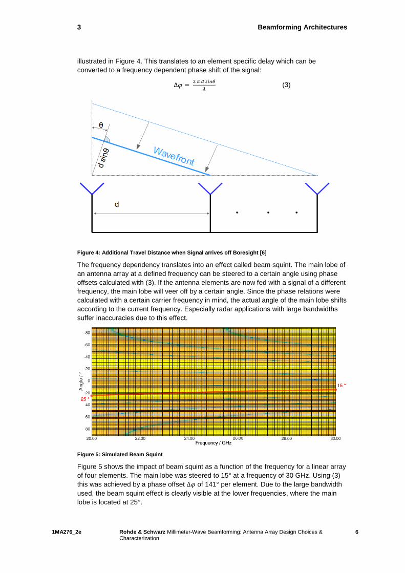
illustrated in Figure 4. This translates to an element specific delay which can be

converted to a frequency dependent phase shift of the signal:

∆𝜑 = 2 𝜋 𝑑 𝑠𝑖𝑛𝜃

𝜆 (3)

Figure 4: Additional Travel Distance when Signal arrives off Boresight [6]

The frequency dependency translates into an effect called beam squint. The main lobe of

an antenna array at a defined frequency can be steered to a certain angle using phase

offsets calculated with (3). If the antenna elements are now fed with a signal of a different

frequency, the main lobe will veer off by a certain angle. Since the phase relations were

calculated with a certain carrier frequency in mind, the actual angle of the main lobe shifts

according to the current frequency. Especially radar applications with large bandwidths

suffer inaccuracies due to this effect.

Figure 5: Simulated Beam Squint

Figure 5 shows the impact of beam squint as a function of the frequency for a linear array

of four elements. The main lobe was steered to 15° at a frequency of 30 GHz. Using (3)

this was achieved by a phase offset ∆𝜑 of 141° per element. Due to the large bandwidth

used, the beam squint effect is clearly visible at the lower frequencies, where the main

lobe is located at 25°.



7

Expression (3) can be converted to a frequency independent term by using time delays

instead of frequency offsets:

∆𝑡 = 𝑑∗𝑠𝑖𝑛𝜃

𝑐 (4)

This means that the frequency dependency is eliminated if the setup is fitted with delay

lines instead of phase shifters. The corresponding receiver setup is shown in Figure 6.

The delay lines 𝑡0 to 𝑡2 compensate for the time delay ∆𝑡, which is an effect of the angle

of the incident wave. As a result, the received signals should be perfectly aligned and will

thus add constructively when summed up.

Figure 6: True Time Delay Beamsteering

The performance of the analog architecture can be further improved by additionally

changing the magnitude of the signals incident to the radiators.

3.2 Digital Beamforming

While analog beamforming is generally restricted to one RF chain even when using large-

number antenna arrays, digital beamforming in theory supports as many RF chains as

there are antenna elements. If suitable precoding is done in the digital baseband, this

yields higher flexibility regarding the transmission and reception. The additional degree of

freedom can be leveraged to perform advanced techniques like multi-beam MIMO. These

advantages result in the highest theoretical performance possible compared to other

beamforming architectures [10].

Figure 7 illustrates the general digital beamforming transmitter architecture with multiple

RF chains.



8

Figure 7: Digital Beamforming Architecture

Beam squint is a well-known problem for analog beamforming architectures using phase

offsets. This is a serious drawback considering current 5G plans to make use of large

bandwidths in the mm-wave band. Digital control of the RF chain enables optimization of

the phases according to the frequency over a large band.

Nonetheless, digital beamforming may not always be ideally suited for practical

implementations regarding 5G applications. The very high complexity and requirements

regarding the hardware may significantly increase cost, energy consumption and

complicate integration in mobile devices. Digital beamforming is better suited for use in

base stations, since performance outweighs mobility in this case.

Digital beamforming can accommodate multi-stream transmission and serve multiple

users simultaneously, which is a key driver of the technology.

3.3 Hybrid Beamforming

Hybrid beamforming has been proposed as a possible solution that is able to combine the

advantages of both analog and digital beamforming architectures. First results from

implementations featuring this architecture have been presented in prototype level, i.e. in

[11].

A significant cost reduction can be achieved by reducing the number of complete RF

chains. This does also lead to lower overall power consumption. Since the number of

converters is significantly lower than the number of antennas, there are less degrees of

freedom for digital baseband processing. Thus the number of simultaneously supported

streams is reduced compared to full blown digital beamforming. The resulting

performance gap is expected to be relatively low due to the specific channel

characteristics in millimeter-wave bands [9].

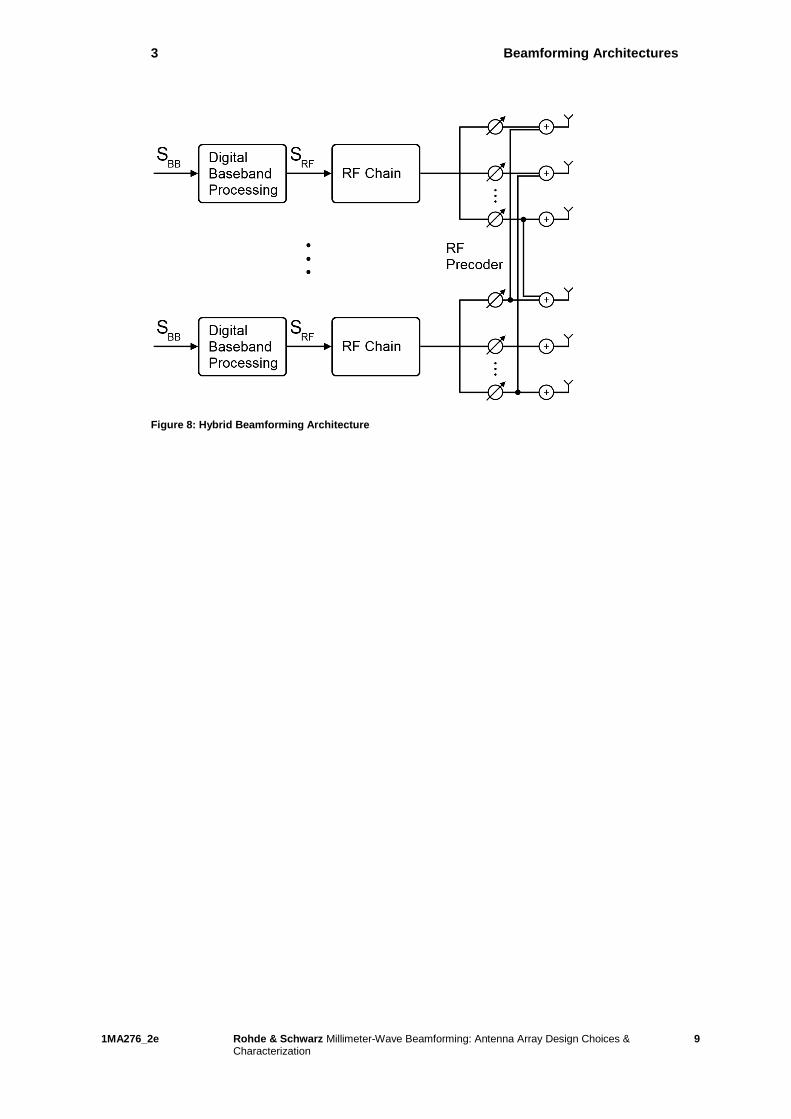
The schematic architecture of a hybrid beamforming transmitter is shown in Figure 8. The

precoding is divided between the analog and digital domains. In theory, it is possible that

every amplifier is interconnected to every radiating element.



9

Figure 8: Hybrid Beamforming Architecture

4 Linear Array Antenna Theory


10


This chapter consists of two sections. The first introduces some theory while the second

section demonstrates the application of these equations by using a suitably chosen

visualization of the results obtained by simulating a linear antenna array of ideal, isotropic

elements.

4.1 Theoretical Background

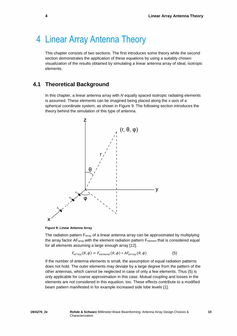
In this chapter, a linear antenna array with N equally spaced isotropic radiating elements

is assumed. These elements can be imagined being placed along the x-axis of a

spherical coordinate system, as shown in Figure 9. The following section introduces the

theory behind the simulation of this type of antenna.

Figure 9: Linear Antenna Array

The radiation pattern Farray of a linear antenna array can be approximated by multiplying

the array factor AFarray with the element radiation pattern Felement that is considered equal

for all elements assuming a large enough array [12].

𝐹𝑎𝑟𝑟𝑎𝑦(𝜃, 𝜙) = 𝐹𝑒𝑙𝑒𝑚𝑒𝑛𝑡(𝜃, 𝜙) ∗ 𝐴𝐹𝑎𝑟𝑟𝑎𝑦(𝜃, 𝜙) (5)

If the number of antenna elements is small, the assumption of equal radiation patterns

does not hold. The outer elements may deviate by a large degree from the pattern of the

other antennas, which cannot be neglected in case of only a few elements. Thus (5) is

only applicable for coarse approximation in this case. Mutual coupling and losses in the

elements are not considered in this equation, too. These effects contribute to a modified

beam pattern manifested in for example increased side lobe levels [1].



11

Aside from the element radiation pattern Felement, the array factor AFarray is required to

calculate Farray according to (5). The linear array factor depends on the wavelength 𝜆, the

angle direction 𝜃, the distance 𝑑 between the elements and the number of elements 𝑁 [1]:

𝐴𝐹𝑎𝑟𝑟𝑎𝑦(𝜃, 𝜙) = ∑ 𝑎𝑛𝑒𝑗𝑛𝑘𝑑 𝑠𝑖𝑛𝜃𝑠𝑖𝑛𝜙𝑒𝑗∆𝜑𝑁𝑛=1 ; 𝑘 = 2 ∗ 𝜋/𝜆 (6)

The complex weighting introduced in chapter 3 can be set using (6). The amplitude

weights are applied per element by the factor 𝑎𝑛. The angle ∆𝜑 calculated with the basic

beam steering formula (3) can be used to steer the beam to an arbitrary angle.

Equation (6) can be simplified by introducing 𝜓, which describes the far-zone phase

difference between adjacent elements [13].

𝜓 = 𝑘𝑑 𝑠𝑖𝑛𝜃𝑠𝑖𝑛𝜙 + ∆𝜑 (7)

Substituting (7) in equation (6) results in:

𝐴𝐹𝑎𝑟𝑟𝑎𝑦(𝜃, 𝜙) = ∑ 𝑎𝑛𝑒𝑗𝑛𝜓𝑁𝑛=1 (8)

The series in (8) can be further simplified and normalized. This leads to the normalized

array factor [13]:

|𝐴𝐹𝑎𝑟𝑟𝑎𝑦(𝜓)| =1

𝑁|

sin (𝑁𝜓/2)

sin (𝜓/2)| (9)

The normalized array factor is periodic in 2𝜋 and allows to infer a lot of information about

the characteristics of the linear antenna array, as will be shown in the next chapter.

4.2 Design Choices

This chapter focuses on the properties of the array factor introduced in the previous

section and the implications for the design of beamforming antennas.

Equation (6) to (9) show that the number of elements and their equidistant spacing have

a great influence on the characteristics of a linear antenna array. The effects of modifying

these two parameters will be explained by the example of Figure 10.

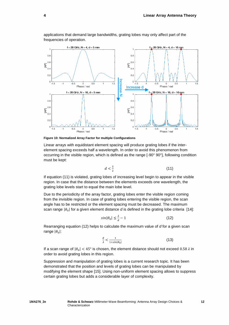
The diagrams on the left show the normalized array factor |𝐴𝐹𝑎𝑟𝑟𝑎𝑦(𝜓)| for an antenna

with an equidistant spacing of 5 mm between elements. The element distance is thus

slightly smaller than 0.5𝜆 at 28 GHz. The normalized array factor of an antenna with a

spacing of 16 mm, which corresponds roughly to 1.5𝜆, is displayed on the right side.

Diagrams on the upper half were calculated for an array of four elements, while the array

factors displayed in the plots on the lower half belong to arrays consisting of 16 elements.

Comparing the upper and lower diagrams of Figure 10 illustrates the effect of increasing

the number of elements while keeping the equidistant spacing constant. The main lobe

width decreases for a larger element count. This means that the more elements a linear

array consists of, the more directivity will be observed. Another effect of increasing the

number of elements is a larger number of side lobes with an overall decrease in level.

The directivity of a linear array can also be improved by increasing the distance between

elements, which produces a narrower main lobe. Similar to a larger number of elements,

the number of side lobes will increase, albeit without a reduced level. On the contrary, a

large inter-element gap produces side lobes that are of equal level compared to the main

lobe. The red dots in Figure 10 highlight this effect for the antenna with a spacing of 1.5𝜆.

The side lobes marked by red dots are called grating lobes. In general these grating

lobes are undesired as energy will be radiated to or received from unwanted directions. In



12

applications that demand large bandwidths, grating lobes may only affect part of the

frequencies of operation.

Figure 10: Normalized Array Factor for multiple Configurations

Linear arrays with equidistant element spacing will produce grating lobes if the inter-

element spacing exceeds half a wavelength. In order to avoid this phenomenon from

occurring in the visible region, which is defined as the range [-90° 90°], following condition

must be kept:

𝑑 <𝜆

2 (11)

If equation (11) is violated, grating lobes of increasing level begin to appear in the visible

region. In case that the distance between the elements exceeds one wavelength, the

grating lobe levels start to equal the main lobe level.

Due to the periodicity of the array factor, grating lobes enter the visible region coming

from the invisible region. In case of grating lobes entering the visible region, the scan

angle has to be restricted or the element spacing must be decreased. The maximum

scan range |𝜃0| for a given element distance d is defined in the grating lobe criteria [14]:

𝑠𝑖𝑛|𝜃0| ≤𝜆

𝑑− 1 (12)

Rearranging equation (12) helps to calculate the maximum value of d for a given scan

range |𝜃0|:

𝑑

𝜆<

1

1+𝑠𝑖𝑛|𝜃0| (13)

If a scan range of |𝜃0| < 45° is chosen, the element distance should not exceed 0.58 𝜆 in

order to avoid grating lobes in this region.

Suppression and manipulation of grating lobes is a current research topic. It has been

demonstrated that the position and levels of grating lobes can be manipulated by

modifying the element shape [15]. Using non-uniform element spacing allows to suppress

certain grating lobes but adds a considerable layer of complexity.



13

4.3 Application Examples

All radiation patterns shown in this section are simulation results that were calculated

using equations (5) and (6). The scripts in appendix 7.1 can be used to generate and

modify these patterns by changing the simulation parameters.

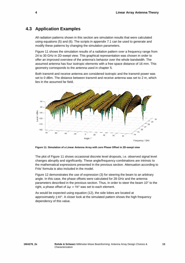
Figure 11 shows the simulation results of a radiation pattern over a frequency range from

24 to 30 GHz in 2D-swept view. This graphical representation was chosen in order to

offer an improved overview of the antenna's behavior over the whole bandwidth. The

assumed antenna has four isotropic elements with a free space distance of 16 mm. This

geometry corresponds to the antenna used in chapter 5.

Both transmit and receive antenna are considered isotropic and the transmit power was

set to 0 dBm. The distance between transmit and receive antenna was set to 2 m, which

lies in the assumed far field.

Figure 11: Simulation of a Linear Antenna Array with zero Phase Offset in 2D-swept view

The plot of Figure 11 shows occasional discrete level dropouts, i.e. observed signal level

changes abruptly and significantly. These angle/frequency combinations are intrinsic to

the mathematical expressions presented in the previous section. Attenuation according to

Friis' formula is also included in the model.

Figure 12 demonstrates the use of expression (3) for steering the beam to an arbitrary

angle. In this case, the phase offsets were calculated for 28 GHz and the antenna

parameters described in the previous section. Thus, in order to steer the beam 10° to the

right, a phase offset of ∆𝜑 = 94° was set to each element.

As would be expected using equation (12), the side lobes are located at

approximately ±40°. A closer look at the simulated pattern shows the high frequency

dependency of this value.



14

Figure 12: Simulation of a Linear Antenna Array with Phase Offset

While the phase offsets of the antenna elements are generally used to determine the

angle of the main lobe, the amplitude weighting provides means to modify the beam width

and side lobe levels. In case of unity amplitude weights ([1, 1, 1, 1]), the main beam width

is smallest.

Decreasing the amplitude levels of the outside elements results in an increased main

beam width. If the weights of the outside elements approach zero ([0, 1, 1, 0]), the

radiation pattern is approximately equal to a two element array with the same

dimensions. The side lobe levels are usually controlled by applying window functions.

Every change of the weights leads to a change in the radiation pattern, while each

window has its own set of advantages and drawbacks [16].

Figure 13 shows the previously discussed effect of different amplitude weights. While the

weighting [1 1 1 1] was used for the simulation shown in Figure 11 and Figure 12, the

weighting factor of the outer elements was reduced to 0.2 in Figure 13. Thus the resulting

weight vector was [0.2 1 1 0.2]. The increased beam width is clearly visible in a direct

comparison between the figures.

Figure 13: Simulation of a Linear Antenna Array with different amplitude weighting



15

Non-equal amplitude weightings are an important instrument for discriminating between

two directions. A small trade-off in terms of directive gain for an intended user may result

in a much larger rejection of unintended signals.

The left of Figure 14 shows the rejection of an unintended user signal at 60° assuming a

signal equal to the one in Figure 11 at 28 GHz is radiated. The red square corresponds to

the rejection at the position of the unintended user. The right part of Figure 14 shows the

effect of unequal amplitude weightings applied to the transmitter. The rejection at the

unintended user increased by approximately 23 dB

Figure 14: Increase in Interferer Rejection through non-equal Amplitude Weights at 28 GHz

5 Linear Array OTA Measurement


16


This chapter will first introduce the effects on the simulated array of using measured data

for the element radiation pattern Felement. Afterwards, the actual over-the-air (OTA)

measurement results obtained from an antenna scan measurement are shown in order to

complement the theoretical calculations.

5.1 Enhancing the Simulation with Measurement Data

5.1.1 Measurement Results for single Elements

The antenna whose elements where measured is a linear array consisting of four

elements with equidistant spacing. Figure 15 shows the superimposed, normalized

radiation patterns of all elements of the antenna at 28 GHz. The measurements were

conducted separately, meaning the other elements were inactive and terminated. Figure

16 shows the level of the main lobe at boresight over the whole frequency range of one

element.

Figure 15: Antenna Element Radiation Pattern



17

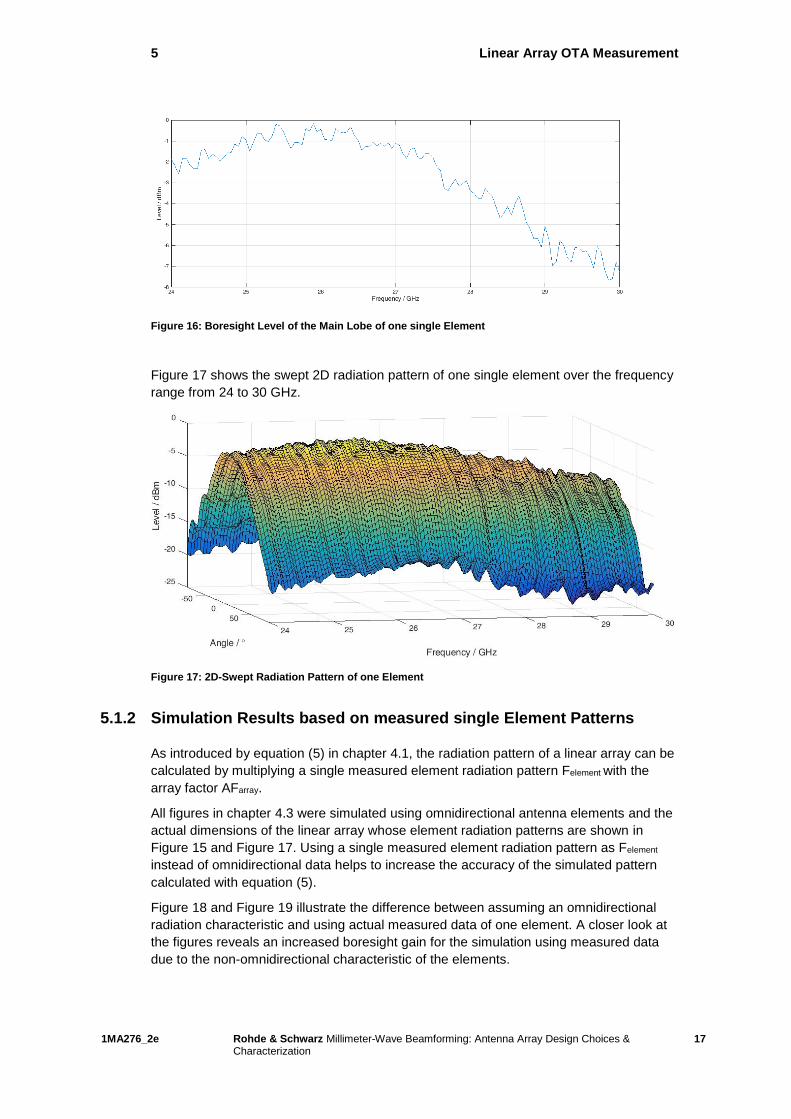
Figure 16: Boresight Level of the Main Lobe of one single Element

Figure 17 shows the swept 2D radiation pattern of one single element over the frequency

range from 24 to 30 GHz.

Figure 17: 2D-Swept Radiation Pattern of one Element

5.1.2 Simulation Results based on measured single Element Patterns

As introduced by equation (5) in chapter 4.1, the radiation pattern of a linear array can be

calculated by multiplying a single measured element radiation pattern Felement with the

array factor AFarray.

All figures in chapter 4.3 were simulated using omnidirectional antenna elements and the

actual dimensions of the linear array whose element radiation patterns are shown in

Figure 15 and Figure 17. Using a single measured element radiation pattern as Felement

instead of omnidirectional data helps to increase the accuracy of the simulated pattern

calculated with equation (5).

Figure 18 and Figure 19 illustrate the difference between assuming an omnidirectional

radiation characteristic and using actual measured data of one element. A closer look at

the figures reveals an increased boresight gain for the simulation using measured data

due to the non-omnidirectional characteristic of the elements.



18

For the simulation, all antenna gains were set to 0 dBi and the element spacing was fixed

at 16 mm in free space.

Figure 18: Simulation with isotropic Elements

Figure 19: Simulation using a single measured Element Radiation Pattern

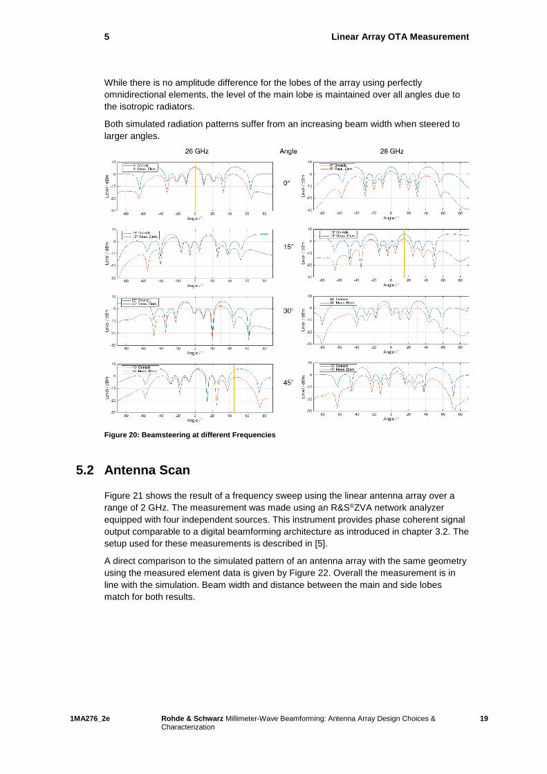
Combining equation (3) and (6) provides means to steer an antenna beam to arbitrary

directions. The effects on the radiation pattern vary depending on the desired angle. As

the beam is steered further away from boresight, the main lobe gets more and more

attenuated while its width increases.

Figure 20 shows these effects for 26 GHz and 28 GHz. The two patterns are the result

from using the measured element pattern (red) and assuming an omnidirectional

characteristic (blue) for the calculations. The yellow vertical line indicates the intended

beam steering direction.

Without any phase difference between the elements, the boresight gain of the measured

elements results in an increased main lobe level in comparison to the side lobes.

Increasing the beam steering angle significantly decreases the amplitude of the main

lobe.



19

While there is no amplitude difference for the lobes of the array using perfectly

omnidirectional elements, the level of the main lobe is maintained over all angles due to

the isotropic radiators.

Both simulated radiation patterns suffer from an increasing beam width when steered to

larger angles.

Figure 20: Beamsteering at different Frequencies

5.2 Antenna Scan

Figure 21 shows the result of a frequency sweep using the linear antenna array over a

range of 2 GHz. The measurement was made using an R&S®ZVA network analyzer

equipped with four independent sources. This instrument provides phase coherent signal

output comparable to a digital beamforming architecture as introduced in chapter 3.2. The

setup used for these measurements is described in [5].

A direct comparison to the simulated pattern of an antenna array with the same geometry

using the measured element data is given by Figure 22. Overall the measurement is in

line with the simulation. Beam width and distance between the main and side lobes

match for both results.



20

Figure 21: Measured Frequency Scan

Figure 22: Simulated Frequency Scan

5.3 Further reading

This section illustrated uniform linear arrays as defined in the introduction. Apart from

budget, the permissible physical size, target band, user application and physical

surroundings for the array determines if a more complex arrangement is feasible.

An introduction to the use of planar arrays, conducted measurements as well as the

choice of waveform properties for steering array antennas is given in reference [17].

6 Results and Outlook


21

6 Results and Outlook

It is already widely accepted that beamforming will play an important role in the

implementation of next generation networks. Many 5G topics are still subjects of ongoing

research, but the general direction taken by the industry includes small as well as large

beamforming arrays, the latter in part only made feasible by the shorter wavelengths

encountered in millimeter-wave bands.

This paper introduced some aspects of beamforming technology from basic signal

propagation to the implementation of a small uniform linear array architecture.

Rohde & Schwarz continues to optimize 5G test solutions for this and other techniques

currently being considered for the 5th Generation in cellular wireless communication.

7 Appendix


22

7 Appendix

7.1 MATLAB® Pattern Generation Script

These MATLAB®1 code excerpts provide functions to generate radiation pattern similar to

those shown in chapter 4.3.

The main function makes use of the two auxiliary functions:

LinearArrayFactor_ElWise for calculating the frequency dependent array factor

depending on the number of elements and complex weights

Friis_Equation returns the free field attenuation depending on the setup and frequency

used.

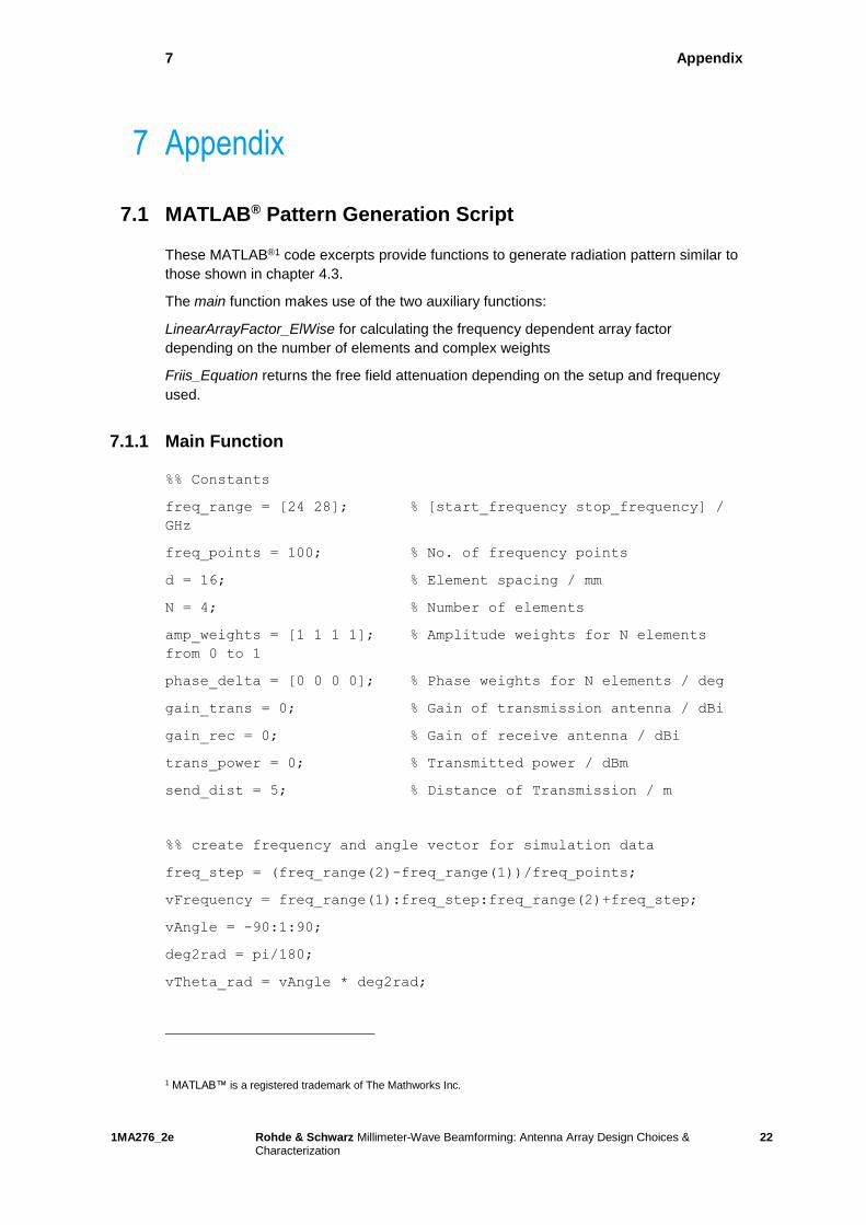
7.1.1 Main Function

%% Constants

freq_range = [24 28]; % [start_frequency stop_frequency] /

GHz

freq_points = 100; % No. of frequency points

d = 16; % Element spacing / mm

N = 4; % Number of elements

amp_weights = [1 1 1 1]; % Amplitude weights for N elements

from 0 to 1

phase_delta = [0 0 0 0]; % Phase weights for N elements / deg

gain_trans = 0; % Gain of transmission antenna / dBi

gain_rec = 0; % Gain of receive antenna / dBi

trans_power = 0; % Transmitted power / dBm

send_dist = 5; % Distance of Transmission / m

%% create frequency and angle vector for simulation data

freq_step = (freq_range(2)-freq_range(1))/freq_points;

vFrequency = freq_range(1):freq_step:freq_range(2)+freq_step;

vAngle = -90:1:90;

deg2rad = pi/180;

vTheta_rad = vAngle * deg2rad;

1 MATLAB™ is a registered trademark of The Mathworks Inc.

7 Appendix


23

%% go through whole bandwidth and calculate the radiation pattern

currfreq = freq_range(1); ii = 1;

while (currfreq <= freq_range(2))

% create omnidirectional characteristic

iPattern = zeros(1,length(vAngle));

% Calculate Array Factor

[AF, ~] = LinearArrayFactor_ElWise(vTheta_rad(:)',

currfreq*1e9, d, N, amp_weights, phase_delta.*deg2rad);

F = 10*log10(AF) + iPattern;

F_real(ii,:) = real(F(:));

% increment counter

ii = ii +1;

currfreq = vFrequency(ii);

end

%% Plot

figure;

surf(vAngle,vFrequency(1:end-1),F_real);

ax = gca;

ax.YAxis.TickLabelFormat = '%,.1g';

set(ax, 'FontSize',12)

rotate3d on;

xlim([-90 90]);

ylabel('\fontsize{14}Frequency / GHz');

xlabel('\fontsize{14}Angle / °');

zlabel('\fontsize{14}Level / dBm');

7 Appendix


24

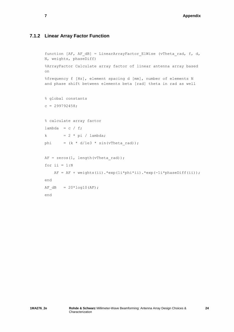
7.1.2 Linear Array Factor Function

function [AF, AF_dB] = LinearArrayFactor_ElWise (vTheta_rad, f, d,

N, weights, phaseDiff)

%ArrayFactor Calculate array factor of linear antenna array based

on

%frequency f [Hz], element spacing d [mm], number of elements N

and phase shift between elements beta [rad] theta in rad as well

% global constants

c = 299792458;

% calculate array factor

lambda = c / f;

k = 2 * pi / lambda;

phi = (k * d/1e3 * sin(vTheta_rad));

AF = zeros(1, length(vTheta_rad));

for ii = 1:N

AF = AF + weights(ii).*exp(1i*phi*ii).*exp(-1i*phaseDiff(ii));

end

AF_dB = 20*log10(AF);

end

References


25

8 References

[1] V. Rabinovich and N. Alexandrov, Antenna Arrays and Automotive Applications:

Springer, 2013, pp. 24-52.

[2] A. Roessler, “5G Waveform Candidates,” Rohde & Schwarz GmbH & Co. KG,

München, 2016.

[3] T. Braunstorfinger, “Phase Adjustment of Two MIMO Signal Sources with Option

B90 (Phase Coherence),” Rohde & Schwarz GmbH & Co. KG, München, 2009.

[4] C. Tröster-Schmid and T. Bednorz, “Generating Multiple Phase Coherent Signals

– Aligned in Phase and Time,” Rohde & Schwarz GmbH & Co. KG, München, 2016.

[5] M. Naseef, G. Lloyd, and M. Reil, “Characterizing Active Phased Array Antennas,”

Rohde & Schwarz GmbH & Co. KG, München, 2016.

[6] ITU-R, Ed., “Attenuation by atmospheric gases: ITU-R P.676-10,” 2013.

[7] J. Butler and R. Lowe, “Beamforming matrix simplifies design of electronically

scanned antennas,” 1961.

[8] C. Powell, “Technical Analysis: Beamforming vs. MIMO Antennas,” 2014.

[9] A. Alkhateeb, J. Mo, N. González-Prelcic, and Heath, Robert W. Jr., “MIMO

Precoding and Combining Solutions for Millimeter-Wave Systems,” IEEE, 2014.

[10] R. Wonil et al., “Millimeter-Wave Beamforming as an Enabling Technology for 5G

Cellular Communications: Theoretical Feasibility and Prototype Results,” IEEE 52,

2014.

[11] X. Gu et al., “W-Band Scalable Phased Arrays for Imaging and Communications,”

IEEE 53, 2015.

[12] M. I. Skolnik, Introduction To Radar Systems: Mcgraw Hill Book Co, 1961, pp.

280-286.

[13] K. S. Das and A. Das, Antenna and Wave Propagation: Tata McGraw Hill

Education Private Limited, 2013, pp. 153-163.

[14] I. V. Minin and Minin Oleg V., Basic Principles of Fresnel Antenna Arrays:

Springer Science & Business Media, 2008, p. 12.

[15] S. I. Nikolov and H. Jensen, “Manipulation of Grating Lobes by Changing Element

Shape,” 34, 2011.

[16] B. Allen and M. Ghavami, Adaptive Array Systems: Fundamentals and

Applications: John Wiley & Sons, 2006, pp. 44 - 52.

[17] M. Kottkamp and C. Rowell, “Antenna Array Testing - Conducted and Over the

Air: The Way to 5G,” München, 2016.

Rohde & Schwarz

The Rohde & Schwarz electronics group offers

innovative solutions in the following business fields:

test and measurement, broadcast and media, secure

communications, cybersecurity, radiomonitoring and

radiolocation. Founded more than 80 years ago, this

independent company has an extensive sales and

service network and is present in more than 70

countries.

The electronics group is among the world market

leaders in its established business fields. The

company is headquartered in Munich, Germany. It

also has regional headquarters in Singapore and

Columbia, Maryland, USA, to manage its operations

in these regions.

Regional contact

Europe, Africa, Middle East +49 89 4129 12345 [email protected] North America 1 888 TEST RSA (1 888 837 87 72) [email protected] Latin America +1 410 910 79 88 [email protected] Asia Pacific +65 65 13 04 88 [email protected]

China +86 800 810 82 28 |+86 400 650 58 96 [email protected]

Sustainable product design

ı Environmental compatibility and eco-footprint

ı Energy efficiency and low emissions

ı Longevity and optimized total cost of ownership

This and the supplied programs may only be used

subject to the conditions of use set forth in the

download area of the Rohde & Schwarz website.

R&S® is a registered trademark of Rohde & Schwarz GmbH & Co.

KG; Trade names are trademarks of the owners.

Rohde & Schwarz GmbH & Co. KG

Mühldorfstraße 15 | 81671 Munich, Germany

Phone + 49 89 4129 - 0 | Fax + 49 89 4129 – 13777

www.rohde-schwarz.com

PA

D-T

-M: 3573.7

380.0

2/0

2.0

5/E

N/

mailto:[email protected]





Date post:	26-May-2018
Category:	Documents
Upload:	buidat
View:	225 times
Download:	0 times

Millimeter-Wave Beamforming: Antenna Array … Beamforming: Antenna Array Design Choices &...

Documents