Millview County Water District - Tracer Study · Web viewMillview County Water District Water...

Millview County Water District

Water System Tracer Study ReportSystem Number 2310006

June 1997

Prepared by

Guy J. Schott, P.E.Associate Sanitary Engineer

Reviewed by

Bruce H. Burton, P.E.District Engineer

California Department of Health ServicesDivision of Drinking Water and Environmental ManagementDrinking Water Field Operations BranchSanta Rosa District

TABLE OF CONTENTS

ABSTRACT...................................................................................................................................

1. INTRODUCTION......................................................................................................................

2. THEORETICAL CONCEPT OF REACTOR MODELS........................................................

2.1. IDEAL PFR................................................................................................................................2.2. IDEAL PFR - IMPULSE INPUT......................................................................................................2.3. IDEAL PFR - STEP INPUT............................................................................................................2.4. IDEAL CFSTR............................................................................................................................2.5. IDEAL CFSTR - STEP INPUT........................................................................................................2.6. IDEAL CFSTR - IMPULSE INPUT..................................................................................................2.7. MULTIPLE CFSTRS....................................................................................................................2.8. MULTIPLE CFSTRS - STEP INPUT................................................................................................2.9. MULTIPLE CFSTRS....................................................................................................................

3. NONIDEAL FLOW PATTERNS..............................................................................................

3.1. E CURVE...................................................................................................................................3.2 F(T) CURVE................................................................................................................................3.3 RELATIONSHIP BETWEEN E AND F(T) CURVES................................................................................

4. MEAN RESIDENCE TIME AND VARIANCE.......................................................................

4.1 MEAN RESIDENCE TIME..............................................................................................................4.2 VARIANCE..................................................................................................................................

5. DISPERSION NUMBER (D/L)..............................................................................................

6. MORRIL INDEX.......................................................................................................................

7. DISINFECTION KINETICS OF MICROORGANISM.........................................................

8. KINETICS OF CHLORINE DECAY.......................................................................................

8.1 EFFECTIVE C X T.........................................................................................................................

9. TRACER TYPE........................................................................................................................

10. T10 VALUE FOR INDIVIDUAL REACTORS.......................................................................

11. EXPERIMENTAL METHOD.................................................................................................

12. TRACER TEST......................................................................................................................

12.1. DATA COLLECTION..................................................................................................................12.2. STEP-INPUT TEST.....................................................................................................................12.3. ANALYTICAL PROCEDURES........................................................................................................12.4. TANKS CONFIGURATIONS AND OPERATIONS...............................................................................

i

TABLE OF CONTENTS

13. RESULTS AND DISCUSSION...............................................................................................

13.1. TANK 1 AND TANKS 1 AND 2 IN SERIES......................................................................................

14. SUMMARY.............................................................................................................................

BIBLIOGRAPHY..........................................................................................................................

APPENDIX A................................................................................................................................

TABLE 5 (CLEARWELLS 1 & 2 IN SERIES).......................................................................................FIG. 16. (F(T) CURVE - TANKS IN SERIES)......................................................................................FIG. 17. (E CURVE - TANKS IN SERIES)..........................................................................................

APPENDIX B.................................................................................................................................

TABLE 6 (CLEARWELL 1)............................................................................................................22FIG. 18. (F(T) CURVE - TANK 1).....................................................................................................FIG. 19. (E CURVE - TANK 1).........................................................................................................

APPENDIX C................................................................................................................................

TABLE 7 (CLEARWELLS 1 & 2 IN SERIES).......................................................................................FIG. 20. (F(T) CURVE - TANKS IN SERIES)......................................................................................FIG. 21. (E CURVE - TANKS IN SERIES)..........................................................................................

APPENDIX D................................................................................................................................

TREATMENT PROCESS.....................................................................................................................

APPENDIX E.................................................................................................................................

INLET/OUTLET CONFIGURATIONS..................................................................................................

ii

Millview County Water District - Tracer Study

Abstract

At the request of the Millview County Water District’s (District) in Millview, California, the Department of Health Services, Drinking Water Field Operations Branch (Department) performed a tracer study analysis to determine the short-circuiting factor (T/T10) for each of two chlorine contact tanks operated in series. Each contact tank has a different volume and inlet/outlet configuration. Without a tracer study, short circuiting factors of 0.3 and 0.2 were assigned to each of the tanks by the Department. The overall short-circuiting factor for the tanks in series was calculated to be 0.24. These short circuiting factors required the District to pre-chlorinate and maintain a higher chlorine residual than desired in order to meet the required disinfection requirement for the inactivation of Giardia cysts.

The objective of the tracer study was to determine if the contact tanks could obtain a higher short-circuiting factor compared to those estimated using United States Environmental Protection Agency (USEPA) guidelines. Results of the tracer study showed that short-circuiting factors of 0.26 (0.3 USEPA) and 0.39 (0.2 USEPA) were hydraulically achieved. The overall short circuiting factor for both tanks in series was 0.34 (0.24 USEPA); an increase of 42 percent.

Theoretical concepts, step dose tracer method, and important considerations for conducting a tracer study are discussed.

1. Introduction

At the request of the Millview County Water District, located in Millview, California, the Department of Health Services, Drinking Water Field Operations Branch conducted a tracer study to determine the short-circuiting factors for two chlorine contact tanks operated in series. The objective was to determine if the contact tanks could obtain a higher short circuiting factor compared to those estimated using USEPA guidelines.

The District owns and operates a community water system in Mendocino County off Highway 101 approximately 60 miles north of Santa Rosa, California. It serves a population of approximately 5,500 people through 1,250 service connections. The treatment facility (Facility) is classified as direct filtration. The District’s water sources are a series of 19 shallow wells and a 6- and 8-inch line in the Russian River. Treatment begins with the injection of gas chlorine and polymer into the incoming raw water. The chemically treated water then goes through coagulation, flocculation, and filtration before entering the contact tanks for further chlorine contact time. Based on direct filtration, the facility is deemed capable of achieving at least 99 percent (2 log) removal of Giardia cysts and a 90 percent (1 log) removal of viruses. One log inactivation of Giardia cysts and 3 log inactivation of viruses is achieved through the District’s disinfection system.

The District’s first chlorine contact tank (Tank 1) in series has an nominal volume of 100,000 gallons. The second tank (Tank 2) in series has a nominal volume of 156,000 gallons. The operating volumes of Tanks 1 and 2 are approximately 87,000 and 136,000 gallons, respectively.

To achieve the inactivation of Giardia cysts and viruses as described above, the raw water is chlorinated at a dose rate to maintain a target free chlorine residual in the water leaving the tanks after an adequate contact time. This is measured as “C x T10”, the free chlorine residual concentration ‘C’ in mg/L, multiplied by the contact time ‘T10’ in minutes. The term T10 is defined as the time it takes for 10 percent of a material to pass through a reactor. Tracer tests provide the most reliable way to estimate the reactor’s T10.

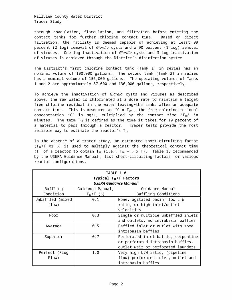
In the absence of a tracer study, an estimated short-circuiting factor (T10/T or ) is used to multiply against the theoretical contact time (T) of a reactor to obtain T 10 (i.e., T10 = x T). Table 1,

Millview County Water DistrictTracer Study

recommended by the USEPA Guidance Manual1, list short-circuiting factors for various reactor configurations.

TABLE 1.0Typical T10/T Factors

USEPA Guidance Manual1

Baffling Condition Guidance Manual, T10/T ()

Guidance Manual Baffling Conditions

Unbaffled (mixed flow) 0.1 None, agitated basin, low L:W ratio, or high inlet/outlet velocities

Poor 0.3 Single or multiple unbaffled inlets and outlets, no intrabasin baffles

Average 0.5 Baffled inlet or outlet with some intrabasin baffles

Superior 0.7 Perforated inlet baffle, serpentine or perforated intrabasin baffles, outlet weir or perforated launders

Perfect (Plug Flow) 1.0 Very high L:W ratio, (pipeline flow) perforated inlet, outlet and intrabasin baffles

The USEPA has developed tables to convert values of the C x T 10 product (mg/L x min) to log inactivation as a function of pH, temperature, and disinfectant concentration. If the C x T 10 product for a water treatment plant meets or exceeds those published in the USEPA tables, then it is assumed that the degree of inactivation has been achieved. Log inactivation achieved through C x T 10 disinfection is then added to log-removal credits based on a system’s current treatment processes to determine whether a public water supply system complies with the Surface Water Treatment Rule (SWTR) treatment requirements. Each system’s compliance status depends on this demonstration. Hence, the methods by which C and T10 are determined are very important.

To estimate the chlorine contact time in tanks with different operating volumes, tank heights, and inlet/outlet configurations is difficult without a tracer analysis. This paper explains the theoretical background of a tracer analysis and the steps involved in conducting a tracer study.

2. Theoretical Concept of Reactor Models

As a first step in the modeling process, it is important to be able to predict the hydraulic performance of a reactor. In predicting hydraulic performance it has become common practice to use models that have been developed to describe the hydraulic characteristics of reactors used to carry out chemical and biological reactions.

The three principal reactor models that are of interest with respect to the tracer study are (1) the plug-flow reactor, (2) the complete-mix reactor, and (3) the cascade of complete-mix reactors. Each reactor is briefly described below.

2.1. Ideal PFR

An ideal plug-flow reactor (PFR) can be either a simple tube or one filled with a packing material to create multiple channels. It is assumed that the flow pattern inside has uniform velocity and concentration in the radial direction at any point along the length of the reactor and there is no longitudinal (axial) diffusional mixing of either reactants or products along the reactor. Although this is an unrealistic assumption for most real-world systems, the PFR is used to define a limit and if desirable can be closely approximated. Because longitudinal mixing does not occur in a PFR, the mean hydraulic detention time (T) is the true hydraulic residence time. 2 Based on this assumption, T10 is equal to the

Page 2


theoretical contact time or the reactor volume divided by its flow rate (V/Q) for a chemical being injected. As described earlier, the term T10 is defined as the time it takes for 10 percent of a material to pass through a reactor. Since plug-flow reactors are not ideal, the actual contact time for a chemical injected into a reactor is less than theoretical. Therefore, T10 will be less than T.

2.2. Ideal PFR - Impulse Input

The assumptions made above allow us to deduce the flow patterns through a PFR, as shown in Fig. 1. A constant flow of water is going through the reactor and a slug of tracer material is added instantaneously (an impulse) to the feed stream as indicated in Fig. 2a. The response as measured by the concentration of a tracer in the fluid leaving the PFR will be that shown in Fig. 2.b, i.e.,. after a delay of one space time, that is t = T, the pulse will come out of the reactor in the same shape as it went in. 2

2.3. Ideal PFR - Step Input

The response of a PFR to a step-input feed of a tracer added at a constant rate to a reactor (with concentration of CAi) is shown in Figures 2.c and 2.d. As described, no tracer will appear leaving a reactor until one space time has passed, at which time the output will change instantaneously to the new condition, i.e., a step function with concentration of CAi. This response of a perfect PFR is not limited to an impulse or step input; no matter what the flow pattern in the feed, the effluent pattern will repeat it exactly after a time delay of one space time.2

Fig. 1.: Plug Flow Reactor

Fig. 2.: Response of a perfect PFR to a Dirac delta (impulse) and a step input: (a) and (b) Impulse response; (c) and (d) Step response.

2.4. Ideal CFSTR

Page 3


Constant-flow stirred-tank reactors (CFSTR) assume instance complete mixing of the material entering the tank. The result is that the concentration of any material leaving the reactor is exactly the same as the concentration at any point in the reactor. An illustrated CFSTR is given in Fig. 3.

The response of an ideal CFSTR to a step or an impulse input of tracer is a little more complicated than the response of the ideal PFR. A materials balance equation, therefore, is written for material A and solved to obtain the flow patterns of an ideal CFSTR. Lets look at a CFSTR with volume, V, receiving a flow of tracer solution at constant flow rate, Q. The unsteady-state mass balance equation for the nonreactive tracer is obtained from Eq. 1.:

V dC A = QCAi - QCA + rAV (rAV = 0 for a nonreactive tracer) (1) dt

Accumulation = Inflow - Outflow + Generation

where CAi and CA are the influent and effluent tracer concentrations.

Fig. 3. CFSTR

2.5. Ideal CFSTR - Step Input

In a step input test, the tracer concentration in the feed is zero initially, C(0) = 0, and then jumps to C Ai

and stays at that value. In response to this step input, the effluent tracer concentration slowly increases to CAi . Equation 1.0 is a first-order linear ordinary differential equation and hence can be integrated to yield Eq. 2.0:2

CA/ CAi = 1 - exp(-t/T) (2)

where T is the theoretical detention time of the reactor, V/Q. The response represented by this equation is shown in Fig. 4. in which it is seen that the effluent tracer concentration starts at zero and asymptotically approaches the ultimate value CAi . Equation 2.0 is a typical first-order system response to a step input. A plot of ln(1 - CA/ CAi ) versus time for a CFSTR should yield a straight line with slope equal to -1/T. This provides a simple means for checking for complete mixing. After one space time, the effluent tracer concentration should be 63.2 percent of the ultimate value. After two and three space times, the effluent tracer concentration should be 86.5 and 95 percent, of the ultimate value, respectively.2

Page 4


Figure 4. Response of a perfect CFSTR to a step and a Dirac delta (impulse) input: (a) and (b) Step response; (c) and (d) Impulse response.

2.6. Ideal CFSTR - Impulse Input

The response to an impulse input at T = 0 (Fig. 4) is formulated by setting QCAi in Eq. 1.0 to be an impulse of mass M of the tracer introduced by Eq. 3.0:2

M (t) - QCA = VdC/dt (3)

The initial condition (t = 0) is zero. Equation 3.0 is a first-order linear ordinary differential equation whose solution is

C = (M/V)exp(-t/T) (4)

The response given by Eq. 4.0 rises immediately to the concentration of M/V and decays exponentially as shown in Fig. 4d. A plot of ln (CA) versus time should result in a straight line with the slope equal to -1/T. After one space time the effluent tracer concentration should be 36.8 % of the initial tracer concentration (M/V). This also provides a simple method for determining whether a reactor approaches complete mixing.2

The impulse response, Eq. 4.0, may be obtained by differentiating the step response, Eq. 2.0, provided the mass of tracer introduced, M, is equal to QCAi.

2.7. Multiple CFSTRs

The number of CFSTRs in series can sometimes approximate one reactor with imperfect mixing. The flow pattern for two CFSTRs in series is given by Eq. 5.0:2

C2/Co = 1 - (1 + t/T)exp(-t/T) (5)

where T = V/Q and C2 is the tracer concentration leaving tank 2. The response from the first tank (given by Eq. 2.0) is the feed to the second tank. By repeating this process for tanks 3, 4, ..., N we can obtain the following expression:2

CN/Co = 1 - [1 + t/T + (t/T)2/2! + .... + (t/T)N-1/(N-1)!] exp(-t/T) (6)

Please note, when using equation 6, CFSTRs in series are of equal volumes. These volumes when summed are equals to the reactor volume being modeled. For example, take a reactor with a capacity of

Page 5


50,000 gallons. If it take five CFSTRs to approximate this reactor, then each CFSTR has a volume of 10,000 gallons.

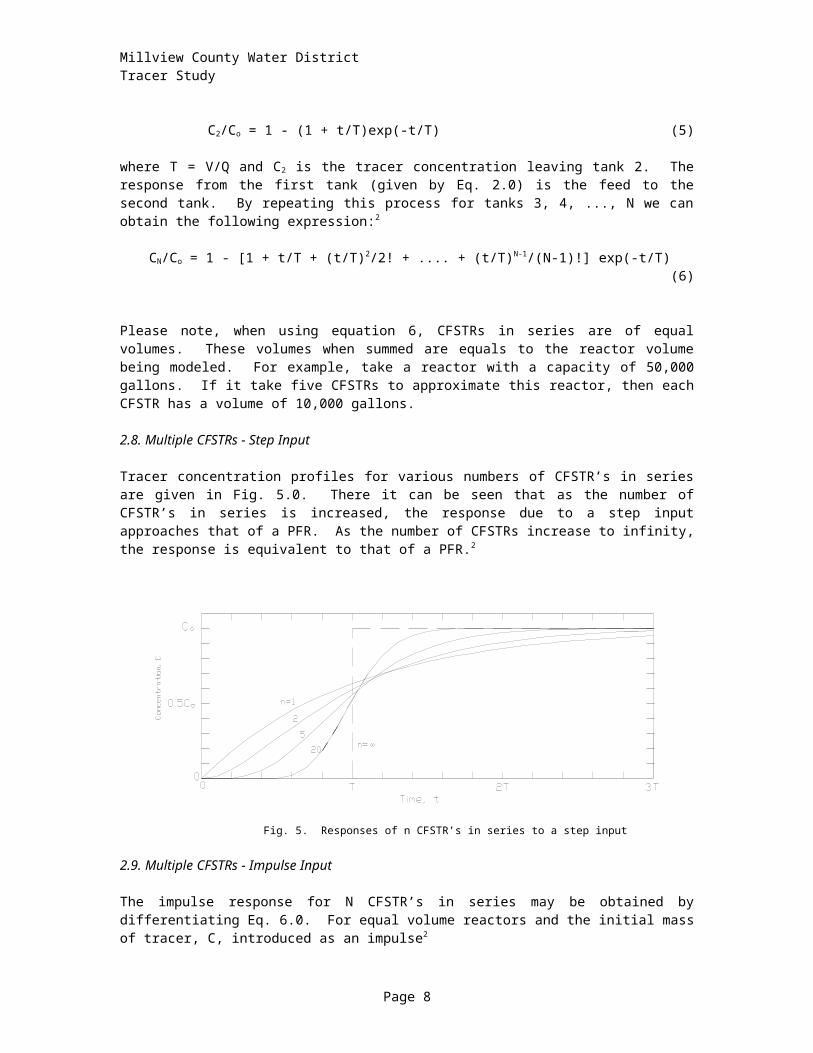
2.8. Multiple CFSTRs - Step Input

Tracer concentration profiles for various numbers of CFSTR’s in series are given in Fig. 5.0. There it can be seen that as the number of CFSTR’s in series is increased, the response due to a step input approaches that of a PFR. As the number of CFSTRs increase to infinity, the response is equivalent to that of a PFR.2

Fig. 5. Responses of n CFSTR’s in series to a step input

2.9. Multiple CFSTRs - Impulse Input

The impulse response for N CFSTR’s in series may be obtained by differentiating Eq. 6.0. For equal volume reactors and the initial mass of tracer, C, introduced as an impulse2

CN = (C/V) [(t/T)N-1/(N-1)!]exp(-t/T) (7)

The impulse responses represented by Eq. 7.0 for various numbers of CFSTR’s in series are shown in Fig. 6. As described in Fig. 6., the addition of a second tank in series reduces the peak and draws out the tracer wave. As more tanks are added, however, the peak concentration increases and moves toward the mean residence time.

Page 6


Fig. 6. Responses of n CFSTR’s in series to a Dirac delta input.

3. Nonideal Flow Patterns

Two idealized flow patterns were described in Section 2; plug flow (in which each fluid element entering the vessel passes through the reactor without intermingling or mixing with other fluid elements) and perfectly mixed flow (in which the each fluid elements down to a molecular scale are completely homogeneous). Though real reactors never fully follow these flow patterns, the deviation from ideal flow can be considerable.1 In the real world, process reactors have flow patterns that lie somewhere between plug-flow and CFSTR. This may be caused by channeling of fluid, by recycling of fluid, or by creation of stagnant regions in the reactor (Fig. 7). In a nonideal reactor, the effluent stream may be looked upon as being made up of fluid elements, which have unique residence times.3

To determine whether a particular model is a good approximation of the fluid flow in an actual reactor, tracer tests are often used. A conservative, nonreactive chemical is introduced into the reactor at the influent, and its effluent concentration is monitored over time. Results of concentration versus time may indicate which model is most appropriate for comparison.

Page 7


Fig. 7. : Nonideal Reactor

There are two common input tracer tests for analyzing flow patterns through reactors: (1) the “impulse-input,” in which the tracer is added all at one time; and (2) the “step-input” procedure, in which the feed of a tracer is abruptly initiated, continued at a fixed rate for a period of three detention and then cut off.

For the step-input method, it has been found that is take approximately three detention times before the concentration leaving a reactor is approximately equal to the concentration of the influence flow into the reactor. As for the impulse-input method, it also takes approximately three detention times before all the mass inputted into a reactor to exit the reactor.

3.1. E Curve As described above, elements of fluid taking different routes through the reactor may require different lengths of time to pass through the vessel. The distribution of these times for the stream of fluid leaving the reactor is called the exit age distribution E, or the residence time distribution RTD of fluid, i.e., the distribution of times required by elements of fluid to pass through the reactor. 3 The E curve is always normalized such that

E= 1 (8)

Thus, E has units of time-1. An E curve is shown in Fig. 8.3

Page 8


Fig. 8. The exit age distribution curve E for fluid flowing through a vessel; also called the residence time distribution, or RTD.

The E(t)dt is the fraction of the effluent that has a residence time between t and t + dt and thus it is the RTD function of the fluid and not mass (Fig. 9.).2

Fig. 9. Fraction of effluent with residence time between t and t+dt.

The E curve can be developed from a pulse-input tracer test by dividing each measured effluent concentration, Ci, by the area under the concentration-time curve, or

Ei = Ci/( Ci ti) (9)

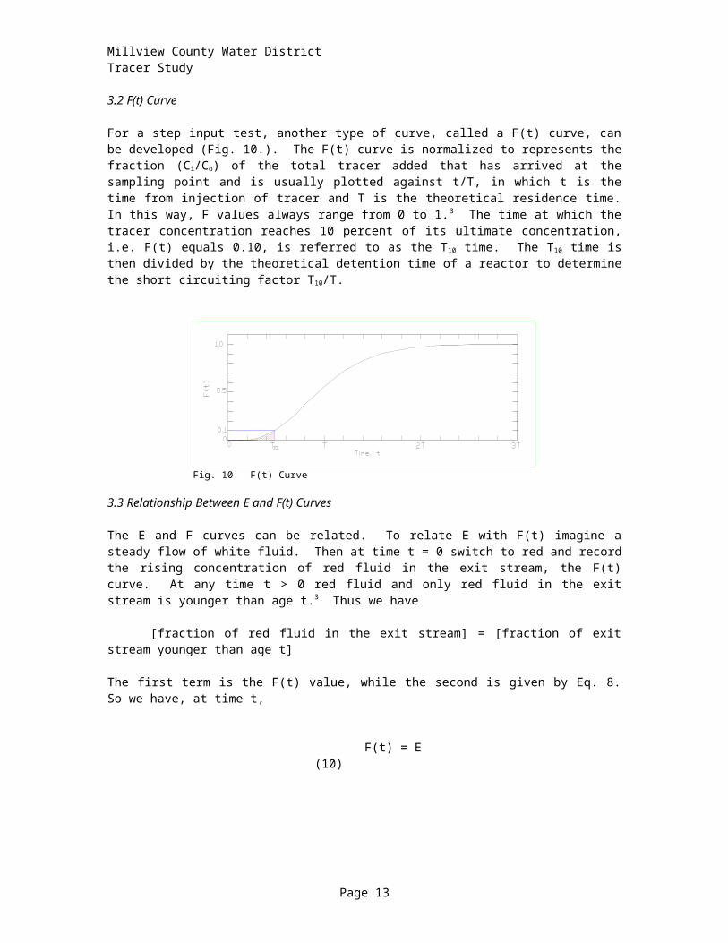
3.2 F(t) Curve

For a step input test, another type of curve, called a F(t) curve, can be developed (Fig. 10.). The F(t) curve is normalized to represents the fraction (C i/Co) of the total tracer added that has arrived at the sampling point and is usually plotted against t/T, in which t is the time from injection of tracer and T is the theoretical residence time. In this way, F values always range from 0 to 1. 3 The time at which the tracer concentration reaches 10 percent of its ultimate concentration, i.e. F(t) equals 0.10, is referred to as

Page 9


the T10 time. The T10 time is then divided by the theoretical detention time of a reactor to determine the short circuiting factor T10/T.

Fig. 10. F(t) Curve

3.3 Relationship Between E and F(t) Curves

The E and F curves can be related. To relate E with F(t) imagine a steady flow of white fluid. Then at time t = 0 switch to red and record the rising concentration of red fluid in the exit stream, the F(t) curve. At any time t > 0 red fluid and only red fluid in the exit stream is younger than age t.3 Thus we have

[fraction of red fluid in the exit stream] = [fraction of exit stream younger than age t]

The first term is the F(t) value, while the second is given by Eq. 8. So we have, at time t,

F(t) = E (10)

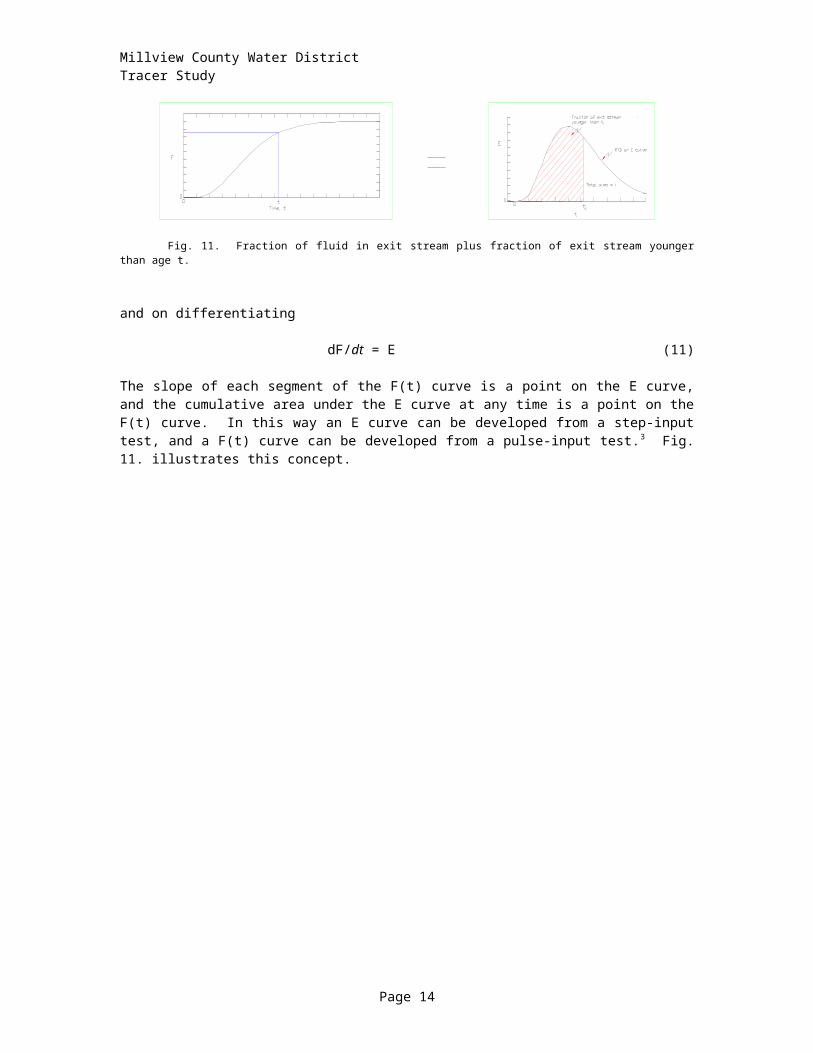
Fig. 11. Fraction of fluid in exit stream plus fraction of exit stream younger than age t.

and on differentiating

dF/dt = E (11)

The slope of each segment of the F(t) curve is a point on the E curve, and the cumulative area under the E curve at any time is a point on the F(t) curve. In this way an E curve can be developed from a step-input test, and a F(t) curve can be developed from a pulse-input test.3 Fig. 11. illustrates this concept.

Page 10


4. Mean Residence Time and Variance

Once the flow through a reactor has been characterized by an E curve, predictions can be made about its behavior. Two important parameters that can be used to characterized the RTD are the mean residence time, tmean and the spread of the curve, which is characterized by the variance 2.2

4.1 Mean Residence Time

If the space time of a reactor is not known, it can be determined experimentally. Since a constant density is assumed for the fluid while it moves through the vessel and isothermal conditions are also assumed, the mean residence time may be expressed by Eq. 12. when used with normalized distributions for closed reactors.2

tmean = ( ti Ei t) (12)

The closer the mean time is to the theoretical detention time, implies less short circuiting and better contact time performance of the reactor.

4.2 Variance

The variance represents the square of the spread of the distribution and has units of (time) 2. When used with normalized distributions for closed reactor it may be expressed by Eq. 13.

2 = (ti2 Ei t - tmean

2) (13)

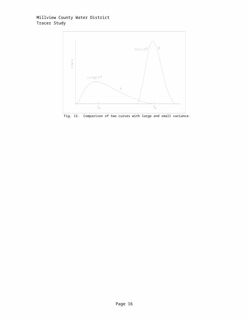
Fig. 12 provides an illustration of two curves, one with a small variance and one with a large variance. The smaller variance again implies less short circuiting within the reactor and improved contact time performance.

Fig. 12. Comparison of two curves with large and small variance.

Page 11


5. Dispersion Number (D/L)

In a plug flow model, a dimensionless parameter called the Dispersion Number (D/L) may be used to characterizes the extent of axial dispersion of a material. The term D is the longitude dispersion coefficient; is the average fluid velocity in the x direction (where x is the distance into the reactor in the direction of flow); and L is the length of the reactor. As D/L approaches zero the dispersion is negligible, hence plug flow. If D/L approaches infinity, the flow is mixed, and the reactor approximates CFSTR. The dispersion number can be found from the variance and mean residence time using Eq. 14. 3

2/t2mean = 2(D/L) - 2(D/L)2(1-exp(-L / D)) (14)

Figure 6 compares the dispersion number for various number of reactor in series.

6. Morril Index

The Morril Index is a statistically parameter for describing a reactor’s hydraulic efficiency. This index is calculated as T90/T10, with both the T90 and T10 values taken from the F(t) curve. Under ideal plug flow conditions, the values T90 and T10 will be approximately equaled to each other causing the Morril Index to approach 1.0.4 As T10/T approaches 1, the lower the Morril Index value will be, indicating improved C x T10 performance.

7. Disinfection Kinetics of Microorganism

The C x t concept was taken from the Chick-Watson law. The USEPA developed this concept into tables which convert values of the C x t product (mg/L x min) to log inactivation as a function of pH, temperature, and disinfectant concentration. Similarity of microbial inactivation by chemical disinfectants to chemical reactions was recognized by Chick. Disinfection is analogous to a bimolecular chemical reaction, with the reactants being the microorganism and the disinfectant. Chick’s law (1908) expresses the rate of destruction of microorganisms by the relationship of a first-order chemical reaction: 5

ln N/No = -kt (15)

where N = number of organism present at time tNo = number of organisms present at time 0 k = rate constant characteristic of type of disinfectant, microorganism, and water quality

aspects of system t = time

Watson (1908) used Chick’s data and refined the equation to produce an empirical relation that includes changes in the disinfectant concentration:5

ln N/No = -k’Cnt (16)

where C = concentration of disinfectantk’ = coefficient of specific lethalityn = coefficient of dilution

The value of n in the Chick-Watson equation depends on the disinfectant and pH value. It is often found to be near unity and hence a fixed value of the product of concentration and time (“C x t product”) results in a fixed degree of inactivation (at a given temperature, pH, etc.).5

The Chick-Watson theory is of limited usefulness in most practical disinfection operations. Most often, the rate of kill does not remain constant. Rather, it increases or decreases with time depending on the type of organism, the changing concentration or form of disinfectant, and other operating condition. 5

Page 12


The C x t concept is based on laboratory batch reactors. However, reactors in water systems are not batch but have flow going in and out of them. Thus, each reactor will have different flow patterns and contact time. Hence, the USEPA built in a factor of safety by using the contact time T 10, which is defined as the time it takes for 10 percent of a material to pass through a reactor.

8. Kinetics of Chlorine Decay

Chlorine is a strong oxidant as well as a powerful disinfectant. Natural waters usually have an oxidant demand because of the inorganic and organic contaminants that are present. Chlorine added to drinking water will be consumed over time. It has been suggested that in some cases the dissipation of chlorine in natural waters can be approximated as a first-order chemical reaction as described in Eq. (18)6.

C = Coexp(-kt) (18)

The term C is the chlorine concentration at time t; C o is the chlorine concentration at time zero; k is the rate constant, time-1; and t is time.

8.1 Effective C x t

If the kinetics of chlorine dissipation are known and the RTD of the reactor vessel can be characterized by a tracer study, this information can be used to give a clearer picture of the actual extent of chlorine contact and its corresponding degree of pathogen inactivation. Using the E curve, each element of fluid can be assumed to be exposed to a different concentration of chlorine for a different amount of time. The concentration to which it is exposed depends on the residence time of that element of fluid. These incremental elements can then be totaled to give an effective C x t. 6 This can be expressed mathematically as

effective C x t = ti Eidt[Coexp(-kti)] (19)

Applying Eq. (19) to data generated from tracer studies at full-scale water treatment plants can lead to a more precise estimate of pathogen inactivation and an indication of the degree to which the SWTR, assuming a conservative application of the concept, under estimates the degree of inactivation.

9. Tracer Type

The type of tracer material used in an approved drinking water system must be nontoxic, approved as a direct additive for drinking water. It is recommended that the tracer chemical be nonreactive in order to provide accurate monitoring of concentrations throughout the study. Typical tracer chemicals for approved drinking water systems are fluoride, calcium chloride, sodium chloride, lithium chloride, and other salts. Recover rates of 90 percent or higher are desirable. Any background concentration detected in the raw water of the tracer used in the study must be taken into account by subtracting the background level from the total concentration during the test.7

10. T10 Value For Individual Reactors

Fig. 13 is an example of two reactors in series where a tracer is injected at the influence line to Tank 1 and samples are taken from the effluent sides of both tanks. The value T10 can be determine from the F(t) curves developed for Tank 1 and for the combined tanks in series. To determine T 10 for Tank 2 (Fig. 13), subtract the calculated T10 value calculated for Tank 1 from the calculated T 10 of combined tanks in series. The difference gives a T10 value for Tank 2. This value can then be divided by its theoretical detention time to give the short-circuiting factor T10/T.

Page 13


Fig. 13. T10 value for individual reactors

11. Experimental Method

The plant tested in this study is a direct filtration treatment plant according to the definition in the SWTR. At the Millview plant, polymer and chlorine is added to the raw water before the in-line static mixer. Zinc-orthophosphate is added after filtration before the clearwells. The two circular clearwell tanks are operated in series and have a combined operating capacity of 223,000 gallons. The working volume for the first clearwell is 87,000 gallons and the second clearwell has a working capacity of 136,000 gallons. At a test flow of 1,750 gpm, the theoretical detention time for clearwells 1 and 2 are 49.7 and 77.7 minutes, respectively. Fig. 14.0 is a schematic of the treatment process for the Millview plant.

Fig. 14. Treatment process train for the Millview County Water District.

Fig. 15. details the inlet and outlet structure for both tanks. The inlet and outlet structure of clearwell 1 are on opposite sides. The inlet and outlet structure of clearwell 2 are 45 degrees from each other. The inlets for both tanks bend at 90o horizontally to the plane. Samples were taken from the outlet of each tank.

Page 14


Fig. 15. Tank configurations.

12. Tracer Test

The step-input tracer test was conducted for the Millview plant. Zinc was used as the tracer for the test because of its current use as a corrosion inhibitor, making it readily available and convenient. It was assumed that the amount of zinc lost in the tanks would be insignificant due to the coating of the tanks by the previous use of zinc-orthophosphate.

12.1. Data Collection

Data collected was time versus the tracer concentration in the effluent of Tanks 1 and 2 during the course of the tracer study analysis. The evaluation of the storage tanks hydraulic performance was completed with a spreadsheet utilizing the following compilations and calculations:

1. Time (t), minutes,2. Time increment between consecutive samples, t, minutes,3. Measured tracer concentration, Ci, mg/L,4. Measured F(t) Curve value, (Ci - Co)/(Cf - Co), where Co is the background concentration of the

tracer and Cf is the final measured concentration of tracer,5. Smoothed F(t) curve determined from a derived equation developed by the Excel spreadsheet,6. E Curve, dF/dt = E, time-1; represents the slope of the respective segment of the F(t) Curve,7. Mid-point of time increment, (ti + ti+1)/2; corresponds to the mid-point of each segment of the

curve for which slope is determined,8. Mean Residence Time, tmean = ( ti Ei t)9. Variance, 2 = ti

2 Ei t - tmean2 , a statistical analysis of dispersion within the tank,

10. Dispersion Number (D/L), iterative solution based on 2/t2

mean = 2(D/L) - 2(D/L)2(1-exp(-L/ D)) and11. Effective C x t = ti Eidt[Coexp(-kti)]

12.2. Step-Input Test

Page 15


The injection of zinc-orthophosphate was discontinued approximately two weeks before the test. This was done to give the contact tanks time to purge any zinc residuals in the water. At the start of the tracer test, time zero, the zinc-orthophosphate feed was turned on. The zinc concentration in the effluent of each tank was monitored over time until the duration of the step-input test was at least 4.7 times the theoretical detention time for tank 1 (228 minutes) and 1.8 times the theoretical detention time for both tanks in series (240 minutes).

The flow rate through the contact tanks and the volume of water in the tanks were kept as constant as possible throughout the test. Due to limited time, only one test was conducted. The tanks were operated at normal capacities. A constant flow rate of 1,750 gpm was maintained throughout the test.

12.3. Analytical Procedures

Zinc samples were analyzed by the Hach DR/2000 using the zincon method by Hach. All samples were collected in paper cups and analyzed immediately. A zinc solution of 0.5 mg/L was prepared and analyzed to determine the accuracy of the Hach DR/2000. The analytical zinc test used has a range 0.00 to 2.00 mg/L as zinc.

12.4. Tanks Configurations and Operations

Tank configurations are presented in Table 2. Plant operating criteria during testing are presented in Table 3.

TABLE 2.0Tank Configurations

Item Tank 1 Tank 2Capacity, gallons 105,800 169,000

Diameter, ft 30 40Sidewall Ht, ft 20 18

Inlet Diameter, inches 12 16Outlet Diameter, inches 12 16

Inlet bend 90 degrees 90 degreesHeight of Inlet, ft 16.7 13.5Height of outlet, ft 0.5 0.5

Outlet location side of wall 7.8 ft from wall, vertical from floorInlet/Outlet Orientation 180 degrees 45 degrees

TABLE 3.0Plant Operating Criteria

Item Tank 1 Tank 2Operating Water Level, ft 16.51 14.51

Operating Capacity, gallons 87,300 136,400Plant Flow Rate, gpm 1,750 1,750

Water Temp., oC 11 11Inlet Velocity, fps 5.0 2.8

Outlet Velocity, fps 5.0 2.8

13. Results and Discussion

Page 16


The step-input test results for Tank 1 and Tanks 1and 2 in series are summarized in Table 4.0

TABLE 4.0Results of step-input test using zinc orthophosphate

Parameter Tank 1 Tank 2 Tanks 1 & 2 togetherFlow Rate, gpm 1,750 1,750 1,750

Theoretical Residence Time, min 50 78 128T10, min 13 30.5 43.5T90, min 77 130 207

Morril Index, T90/T10 13.5 4.3 5.4Mean Residence Time, min 62 - 98.7SWTR C x T10 ,mg-min/L 21 49 70Effective C x t, mg-min/L 96 - 163

T10/T 0.26 0.39 0.34SWTR, T10/T 0.3 0.2 0.24

Effective C x t/ SWTR C x T10 4.6 - 2.3

13.1. Tank 1 and Tanks 1 and 2 in Series

One tracer test was conducted at the Millview County Water District. The step-input method was used for this study. A step-input curve was developed for Tank 1 and for both tanks in series. The F(t) curves are presented in Figures 16 and 18 in the Appendix.

The F(t) curves were developed by dividing the corrected effluent concentrations (after subtracting the background zinc concentration) by Co the concentration measured at the end of test for each tank.

Values for T10 and T90 were obtained graphically from each F(t) curve. These are summarized in Table 4. The theoretical residence times (volume/flow rate) are shown for comparison. Values for T 10 and T90

were calculated based on Section 10.

The ratio T10/T for both tanks in series was determined to be 0.34. The ratio T 10/T for Tanks 1 and 2 individually were 0.26 and 0.39, respectively. The T10/T ratio for Tank 1 is in the range suggested in the USEPA guidance manual. However, the T10/T ratio for Tank 2 was much higher compared to the suggested USEPA value. Calculated results are shown in the Appendix (Tables 5 and 6).

The E curves were generated from the F(t) curves. The E curves were used to calculate the mean residence time, variance, and effective C x t as shown in the Appendix (Fig 17 and 19). The values calculated for the mean residence times are within 77 to 80 percent of the theoretical times, as shown in Table 2. The values for the mean and variance were then used to determine the number of CFSTRs in series that would best fit the tracer data. The number of CFSTRs calculated for both tanks in series was between three and four. One CFSTR was the best fit curve for Tank 1. These points are plotted on the F(t) curves shown in the Appendix.

The Dispersion numbers were calculated using Eq. 14. For tanks in series, D/L was calculated to be 0.164, a rather high dispersion number (Fig. 6). The exit stream of Tank 1, D/L was calculated to be 2.5, an extremely high dispersion number (Fig. 6) suggesting good mixing.

To determine the effective C x t values, a rate constant, k for chlorine decay was determined. The dissipation of chlorine in water was assumed to approximate a first-order chemical reaction, using Eq. 18:

C = Coexp(-kt)

Page 17


where C = chlorine concentration at time t, Co = chlorine concentration at time zero, k = decay rate constant with units time-1, and t = time in minutes. Taking the natural logarithm of both sides of Eq. 18 and writing the equation in the form of line yields Eq. 20:

ln(C) = -kt + ln(Co) (20)y = mx + b

where k is the slope of the line.

For this study an initial chlorine concentration (Co) of 2.0 mg/L was used. By monitoring the decrease of chlorine residual of a sample through time, the decay rate constant (k) was graphically determined to be 0.0023.

After the rate constant was determined, the effective C x t values were calculated using Eq. 19. The last column for each table of results in the Appendix presents the calculations for the test. The sum of these columns represents the effective C x t. At the bottom of each table contains the effective C x t value and the C x T10 value calculated in accordance with the SWTR. In this test, the effective C x t values are significantly greater than the minimum C x T10 values allowed by the SWTR. This suggest the degree of inactivation is probably much greater.

The final zinc concentrations for Tanks 1 and 2 were 1.27 and 1.12 mg/L which should be approximately the same. This discrepancy is probably due to the fact that the tracer study did not run long enough to achieve at least a three detention for both tanks in series. Tank 1 achieve a run time of 4.6 times its theoretical detention time and 1.8 for both tanks in series (Tables 5 and 6). If we assume that the final zinc concentration for Tank 2 would have been equal to Tank 1 if the tracer study was ran longer, a higher T10/T would theoretically be achieved. A new F(t) and E curve was plotted for both tanks in series using the final concentration for Tank 1 (Fig. 19 & 20), Appendix. The revised calculated results are obtained in Table 7.

14. Summary

Tracer tests have been demonstrated to be a very effective method of characterizing the behavior of flow through process units in water treatment facilities. Residence time distributions can be used to characterize flow behavior of a reactor. Although the USEPA guidance for the SWTR recommend that T10 be used to determine the contact time of the disinfectant, additional information about flow behavior and hydraulic effectiveness of process units can be gained by using the entire residence time distribution.

Table 4 is a summary of the tracer tests discussed. The short-circuiting factor T 10/T for Tank 2 almost doubled when compared with the T10/T initially assigned. The T10/T for Tank 1 was slightly less than previous assigned value based on the USEPA guidelines.

Tank 2 had a significantly higher ratio of T10 to T compared with Tank 1. The most significant differences between the tanks were the inlet/out arrangements, working volumes, and the inlet/outlet velocities. Tank 1’s outlet is on the bottom side wall of the tank directly across (180 o) from the inlet and approximately 16 feet below it. Tank 2’s outlet is on the bottom of the tank, approximately 45 o from the inlet pipe (counterclockwise) and approximately 13 feet below it. See the inlet/outlet configuration diagram in Appendix E. Both inlet pipes entered the tanks perpendicular to the wall then were turned 90 o

by an elbow so the water entered the tank traveling parallel to the wall and water surface. The inlet water direction tended to set up a circular current in the tanks making the path of the water traveled to the outlet in Tank 2 longer than in Tank 1. This could partially account for the larger T 10/T achieved by Tank 2.

Tank 1’s working volume was approximately 37 percent smaller than Tank 2 but its inlet velocity was approximately 80 percent higher than that of Tank 2. The higher velocity water stream combined with the shorter physical distance around the circumference of the tank would allow more short circuiting to occur in Tank 1 than in Tank 2, resulting in a lower T10/T factor for Tank 1.

Page 18


The effective C x t for the tanks in series was determined using the kinetics of chlorine concentration decay and each tanks RTD. The results indicated that a substantial margin of safety in the degree of pathogen inactivation is built into the SWTR under the most conservative interpretation. For both tanks, the effective C x t was significantly higher, by a factor of up to four times, than the minimum C x t allowed by the SWTR, i.e., Ceffluent x T10. These higher effective C x t values imply a higher degree of virus and Giardia cysts inactivation. It should be noted that the effective C x t was based on the assumed kinetics of chlorine decay, which can change with change in water quality.

Zinc was used as a tracer in this study. There was no facility to determine the zinc dose rate to verify the maximum effluent concentration of zinc measured out of Tank 1 was approximately the same as the influent to Tank 1. This would be necessary to determine if any zinc lost occurred in the tanks. If possible, a sample tap should be installed on the influent of a reactor being modeled for any tracer study to determine its dose rate. If this test were to be run again, sodium fluoride would be the choice of tracer.

To perform a successful tracer study, detailed planning must be done. Some of the important aspects that should be considered are 1) type of tracer test (slug or step-input), 2) choice of tracer, 3) tracer addition, 4) chemical dose rate, 5) plant operating conditions during the test, 6) sample collection points, 7) sampling intervals, and 8) data analysis.

The tracer study for the Millview County Water District generated good data and valuable information. The objective of this study was to determine if the contact tanks could obtain a higher short circuiting factor than previously assigned by the Department. The study proved that the tanks in series can achieve a higher short-circuiting factor than previous estimated. This increase was calculated to be 42 percent.

REPORT PREPARED BY: REVIEWED BY:

GUY J. SCHOTT, P.E. BRUCE H. BURTON, P.E.ASSOCIATE SANITARY ENGINEER DISTRICT ENGINEER

Page 19


BIBLIOGRAPHY

1. U.S. EPA, Guidance Manual for Compliance with the Filtration and Disinfection Requirements for Public Water Systems Using Surface Water Sources, American Water Works Association, Denver, Co., 1991.

2. Grady, C. P. Leslie Jr. & Lim, Henry C., Biological Wastewater Treatment, Marcel Dekker, Inc., New York, 1980.

3. Levenspiel, Octave, Chemical Reaction Engineering, Wiley & Sons, Inc., New York, 1972.

4. American Water Works Association, Water Quality and Treatment, Fourth Edition, McGraw-Hill, Inc.

5. Montgomery James M., Consulting Engineers, Inc., Water Treatment Principles and Design, John Wiley & Sons, New York, 1985.

6. Teefy, Susan M. & Singer, Philip C., Performance and Analysis of Tracer Tests to Determine Compliance of a Disinfection Scheme With the SWTR, Journal AWWA, December 1990.

7. Bishop, Mark M; Morgan, J Mark; Cornwell, Brendon; & Jamison, Donald K, Improving the Disinfection Detention Time of a Water Plant Clearwell, Research & Technology, March 1993.

file: 2310006/Tracer/Tracer_M.Doc

Page 20


APPENDIX A

Table 5 (Clearwells 1 & 2 in Series)Fig. 16. (F(t) Curve - Tanks in Series)Fig. 17. (E Curve - Tanks in Series)

Page 21


APPENDIX B

Table 6 (Clearwell 1) Fig. 18. (F(t) Curve - Tank 1)Fig. 19. (E Curve - Tank 1)

Page 22


APPENDIX C

Table 7 (Clearwells 1 & 2 in Series)Fig. 20. (F(t) Curve - Tanks in Series)Fig. 21. (E Curve - Tanks in Series)

for assumed zinc concentration at 1.27 mg/L

Page 23


APPENDIX D

Treatment Process

Page 24


APPENDIX E

Inlet/Outlet Configurations

Page 25

Date post:	01-Apr-2018
Category:	Documents
Upload:	ngohanh
View:	212 times
Download:	0 times

Millview County Water District - Tracer Study · Web viewMillview County Water District Water...

Documents