1

Modeling Long Overnight Trips by Chaining Recreation Sites

Min Chen

Michigan State University

chenmin5@msu.edu

Frank Lupi

Michigan State University

lupi@msu.edu

Selected Paper prepared for presentation at the Agricultural & Applied Economics

Association’s 2013 AAEA & CAES Joint Annual Meeting, Washington, DC, August 4-

6, 2013.

Copyright 2013 by Chen and Lupi. All rights reserved. Readers may make verbatim

copies of this document for non-commercial purposes by any means, provided that this

copyright notice appears on all such copies.

2

1 Introduction

In recreation studies, valuation often applies to trips where the primary objective is

recreation and only one site is visited, so day trip data is the most widely used as it

normally meets the two requirements (Caulkins et al (1986), Lew and Larson (2005),

Moeltner and Shonkwiler (2005), Scarpa and Thiene (2005), Smith (2005), von Haefen et

al (2005), Kim et al (2007), Timmins and Murdock (2007), Parsons et al (2009)). Some

studies, most of which are for fishing or hunting, do not explicitly provide complete trip

detailsbut single-objective and single-site assumptions are still imposed (Englin and

Shonkwiler (1995), Haab and Hicks (1997), Provencher and Bishop (1997), Schuhmann

and Schwabe (2004), Morey et al (2006), Cutter et al (2007), Hynes et al (2007), Haab et

al (2008), von Haefen and Phaneuf (2008)).

Nonetheless, a nontrivial portion of recreation trips, especially those lasting more

than a day, either have multiple objectives, involve multiple sites, or both. Demand for

recreation activities will be more accurately valued if these trips are accounted for. There

have been studies investigating these issues directly or indirectly. For example, Kealy and

Bishop (1986) included the total number of recreation days as the dependent variable in

their travel cost demand model. The average number of days per recreation trip was

assumed to be one exogenous independent variable. Other factors included individual

characteristics, monetary travel cost, daily on-site costs, daily overnight expenditures, etc.

Mendelsohn et al (1992) had major combinations of sites and treated one multiple-site

trip as a trip to one of those site combinations. People could substitute across individual

sites and site combinations. Hoehn et al (1996) proposed a four-level nested logit model

for fishing trips to take into account trip duration as well as locations and target species.

3

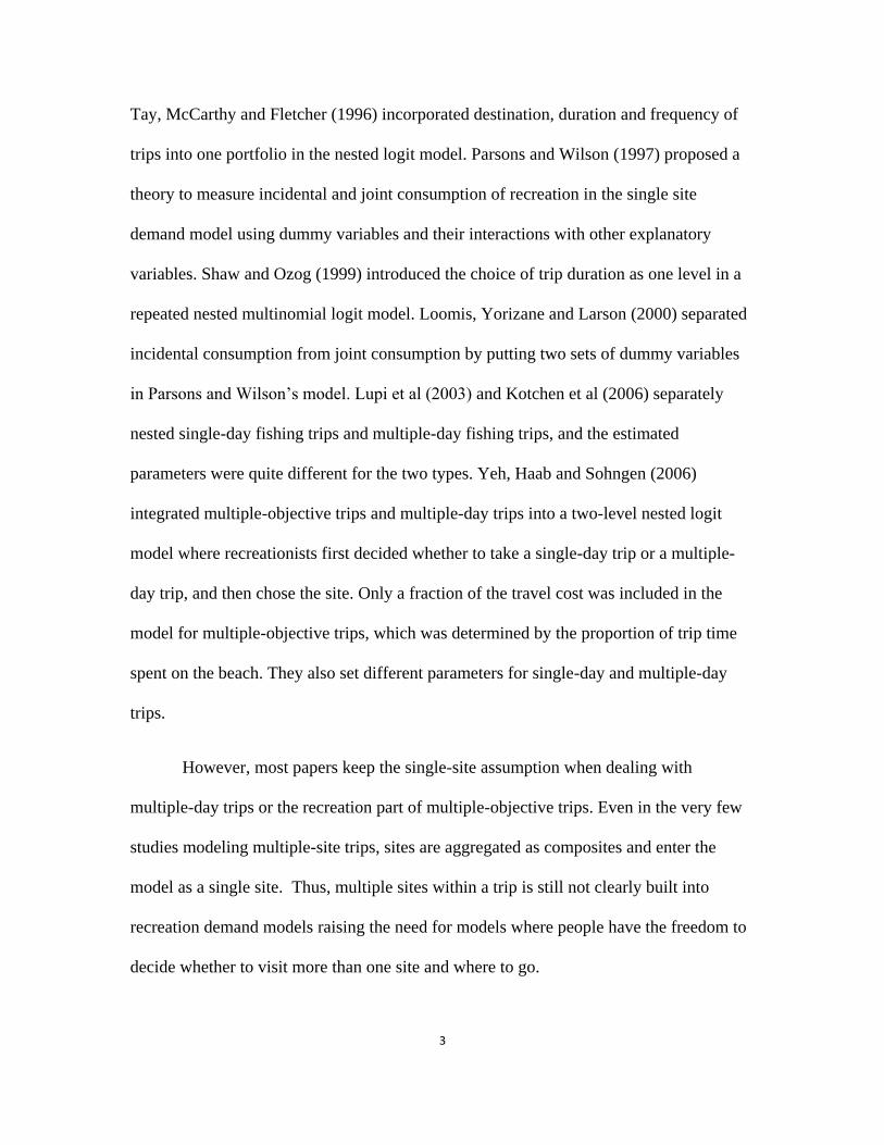
Tay, McCarthy and Fletcher (1996) incorporated destination, duration and frequency of

trips into one portfolio in the nested logit model. Parsons and Wilson (1997) proposed a

theory to measure incidental and joint consumption of recreation in the single site

demand model using dummy variables and their interactions with other explanatory

variables. Shaw and Ozog (1999) introduced the choice of trip duration as one level in a

repeated nested multinomial logit model. Loomis, Yorizane and Larson (2000) separated

incidental consumption from joint consumption by putting two sets of dummy variables

in Parsons and Wilson’s model. Lupi et al (2003) and Kotchen et al (2006) separately

nested single-day fishing trips and multiple-day fishing trips, and the estimated

parameters were quite different for the two types. Yeh, Haab and Sohngen (2006)

integrated multiple-objective trips and multiple-day trips into a two-level nested logit

model where recreationists first decided whether to take a single-day trip or a multiple-

day trip, and then chose the site. Only a fraction of the travel cost was included in the

model for multiple-objective trips, which was determined by the proportion of trip time

spent on the beach. They also set different parameters for single-day and multiple-day

trips.

However, most papers keep the single-site assumption when dealing with

multiple-day trips or the recreation part of multiple-objective trips. Even in the very few

studies modeling multiple-site trips, sites are aggregated as composites and enter the

model as a single site. Thus, multiple sites within a trip is still not clearly built into

recreation demand models raising the need for models where people have the freedom to

decide whether to visit more than one site and where to go.

4

We address the issue by modeling the demand for beach sites on multiple day

trips that can include either one or two sites visited per trip. The data was obtained

through two surveys, a screener mail survey and a follow-up web survey, which were

conducted in 2011 and 2012 to Michigan residents asking about visitation to public Great

Lakes beaches. In the web survey, we asked people to report up to three beaches on one

randomly selected trip lasting four nights or more on which they spent the most/second

most/third most amount of time. With this information, we are able to investigate whether

the results of multi-site demand models are significantly different when modeling only

the primary destination and allowing multiple destinations for overnight trips.

2 Survey and Data

2.1 Screener Mail Survey

The purpose of the screener survey was to recruit people who participated in beach

recreation. The sample was drawn from the State of Michigan driver license list. People

who live in the Upper Peninsula are excluded as the majority of population lives in the

Lower Peninsula. The original sample size was 32,230, and the number goes down to

29,613 after removal of deceased people and those with bad mailing addresses.

The questionnaire had three parts. The first part asked people about their

participation in various everyday activities, recreation activities and indoor activities.

Only one screener question was about Great Lakes beaches in order to reduce self-

selection bias. The second part of the screener was about participation obstacles, such as

5

time or money constraints. The third part contained demographic questions like race,

education, employment status, and household income.

From June, 2011 to November, 2011, three waves of survey packages were

mailed out and two waves of automated phone calls were sent to household landlines as

reminders. 11,028 people returned their questionnaires for a 37.24% response rate. 9,591

respondents were kept for data analysis according to the criteria of living in the Lower

Peninsula and being the addressees, among which 5,556 said they have visited a Great

Lakes beach since June 1, 2010.

2.2 Web Survey

The 5,476 respondents that participated1 in beach recreation from the screener mail

survey were invited to a follow-up web survey on Great Lakes beaches. There were an

additional 85 participants (their responses were received after the mail survey was closed

for data collection) chosen for a pilot survey, the purpose of which was to test the

functionality and data storage of the web survey.

There were two sections in the web survey, the beach trip section and the choice

experiment section. In the beach trip section, following the survey in Parsons et al (2009),

trips were categorized into three types: trip lasting a day or less (day trip), overnight trip

of less than four nights (short overnight trip), and overnight trip of four nights or more

(long overnight trip). People were asked to report trip numbers of each type during the

1 Due to some data manipulation errors, the sample size is less than the number of participants in beach

recreation.

6

time frame from Memorial Day weekend, 2011 to September 30, 2011 (the primary

beach-going season). For day and short overnight trips, detailed questions were asked for

up to two randomly selected trips; for long overnight trips, information was collected on

one randomly selected trip about where people go and how long they stay at each beach.

In the choice experiment section, after information treatments, three pairs of hypothetical

beaches with randomly drawn attributes were presented for people to choose (Weicksel

(2012)). Questions on general perceptions of public beaches on each Great Lake follow

the choice experiments. Demographic questions conclude the web survey.

Four waves of contacts were sent to potential web respondents. The first wave

mail package included an invitation letter and a $1 cash incentive; postcard reminders

were used in the second and third waves, differing in sizes. In the last wave, an incentive

strategy based upon completion of the survey was implemented. Also, people without

internet access were asked to return a small postcard mailed together with the letter. The

survey started in April, 2012, and closed right after the Memorial Day weekend, 2012. In

total, 3,197 people logged on the survey and answered our initial trip questions, giving a

response rate of 58.38%.

2.3 Data

There are 588 public Great Lakes beaches in Michigan. To model trips with multiple

destinations, it will be extremely computationally burdensome to construct the choice set

with individual beaches. According to literature on site aggregation (Lupi and Feather

(1998), Haener et al (2004), etc.), we aggregate the 588 public beaches into 49 beach

7

areas, where the two key factors to consider are beach popularity and geographic

distribution (see Figure 1 and Figure 2). A beach is more likely to stand on its own if

many people go there. Beaches with no visits are dropped. Since the parameter estimate

for travel cost is the denominator of all welfare estimates, to minimize the distance

heterogeneity in all beach areas, we keep the average distance between two individual

beaches under 18 miles within one area. Characteristics of these beach areas are averages

of individual beach characteristics.

Figure 1: Public Great Lakes Beaches with Visits2

2 Figure 1, 2 and 3 are google earth images. File conversion is through the website:

http://www.earthpoint.us/ExcelToKml.aspx

8

Figure 2: Aggregated Beach Areas in the Multiple Day Trip Models

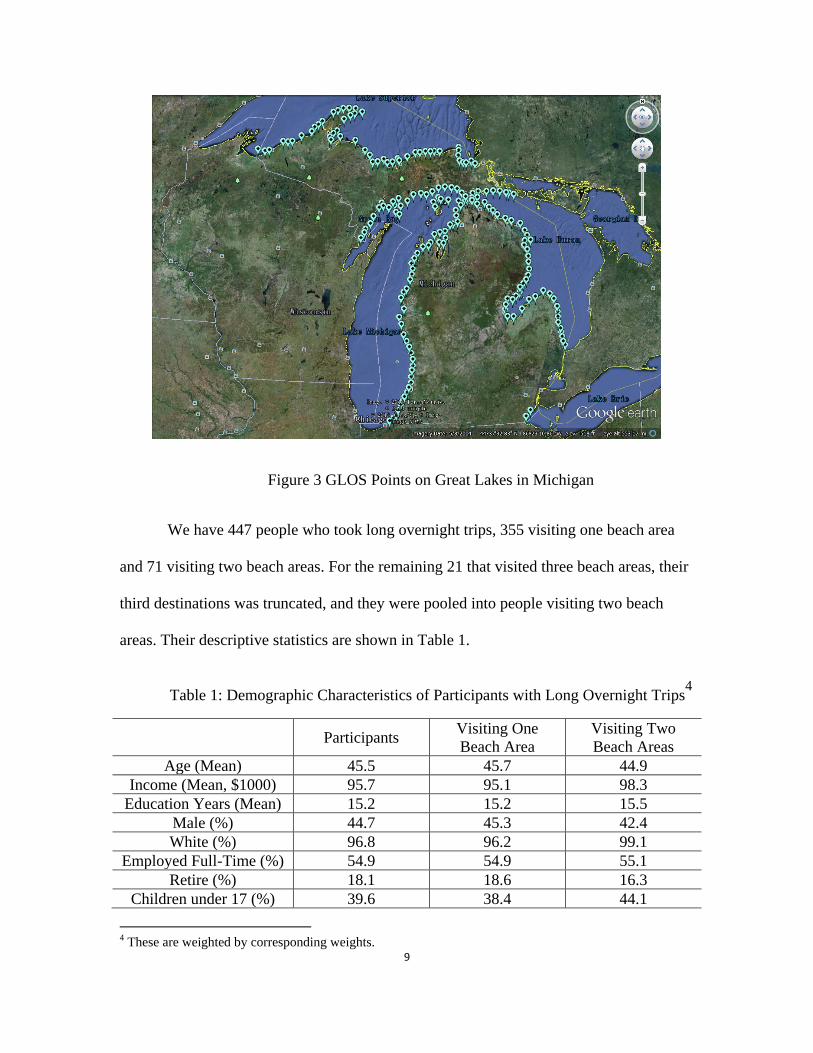
Individual beach length information was provided by Michigan Department of

Environmental Quality. Data on water surface temperature was obtained from the

National Oceanic and Atmospheric Administration (NOAA) Great Lakes Environmental

Research Laboratory (GLERL) using the Great Lakes Observing System (GLOS) Point

Query tool3. 50 grid points were selected on Lake Superior along the coastline, 56 on

Lake Huron, 79 on Lake Michigan and 2 on Lake Erie as in Figure 3. Daily temperatures

were retrieved at these points and averaged into monthly temperatures. Monthly data was

directly used for Lake St. Clair as its daily data is not available on-line. Individual

beaches in the site choice models were matched to the nearest location with temperature

data.

3 http://glos.us/data-tools/point-query-tool-glcfs

9

Figure 3 GLOS Points on Great Lakes in Michigan

We have 447 people who took long overnight trips, 355 visiting one beach area

and 71 visiting two beach areas. For the remaining 21 that visited three beach areas, their

third destinations was truncated, and they were pooled into people visiting two beach

areas. Their descriptive statistics are shown in Table 1.

Table 1: Demographic Characteristics of Participants with Long Overnight Trips4

Participants Visiting One

Beach Area

Visiting Two

Beach Areas

Age (Mean) 45.5 45.7 44.9

Income (Mean, $1000) 95.7 95.1 98.3

Education Years (Mean) 15.2 15.2 15.5

Male (%) 44.7 45.3 42.4

White (%) 96.8 96.2 99.1

Employed Full-Time (%) 54.9 54.9 55.1

Retire (%) 18.1 18.6 16.3

Children under 17 (%) 39.6 38.4 44.1

4 These are weighted by corresponding weights.

10

3 Models

A repeated nested logit model is used for seasonal visitation. Figure 4 shows the

traditional approach to model overnight trips. In one choice occasion, a person either

does not take a trip, or spends all the time on one beach.

Figure 4: Decision Tree with Primary Destination

To incorporate multiple destinations in the trip, as illustrated in Figure 5, if taking

a long overnight trip, a person can visit one beach or two beaches. In the nest of visiting

two beaches, the first level of beaches represents the primary destination; the second level

of beaches contains all other beaches in the choice set.

11

Figure 5: Decision Tree with Multiple Destinations

In occasion t, if a person n takes a long overnight trip and visits two beaches, the

conditional probability to choose j as the secondary beach after visiting beach k is:

( | )

∑

k-1 means beach k is excluded from the choice set for the secondary beach.

The conditional probability that a person n chooses k as the primary beach is:

( | ) (∑

)

∑ (∑

)

If a person n visits one beach, the conditional probability to choose beach i is:

12

( | )

∑

The conditional probabilities of visiting two beaches and visiting one beach are:

( | ) (∑ (∑

) )

(∑ (∑

) ) (∑

)

( | ) (∑

)

(∑ (∑

) ) (∑

)

Denote the representative utility of not taking a long overnight trip as ,

then the probabilities of taking a long overnight trip and not taking a long overnight trip

are:

( ) ((∑ (∑

) ) (∑

) )

((∑ (∑

) ) (∑

) )

( )

((∑ (∑

) ) (∑

) )

Then the unconditional probabilities of choosing the pair of beach k and j and

choosing beach i only are:

13

( ) ( | )

( | )

( | ) ( )

(∑

)

(∑ (∑

)

)

((∑ (∑

)

)

(∑

)

)

((∑(∑

)

) (∑

) )

( ) ( | )

( | ) ( )

(∑

)

((∑ (∑

)

)

(∑

)

)

((∑(∑

)

) (∑

) )

We only know where people went on one randomly selected trip, but we have

them report the numbers of long overnight trips taken in each month. Therefore, the

likelihood function is:

14

∏∏ ( )

∏∏∏ ( )

∏∏( ( ) ( )

)

Where T is the total number of choice occasions, 5 per month in our case; N is the total

number of people who take long overnight trips, where people visit one beach only

and people visit two beaches. y and w are binary indicators.

If one visits on beach, includes travel cost and time cost as the price variable,

and beach length, monthly water temperature and regional dummies as the quality

variable.

Based on Champ et al (2003). the computation of total trip cost is:

( ⁄ ) ( ⁄ )

$0.476 per mile is the driving cost for an average size car. This number coms from annual

report of the American Automobile Association (AAA), and excludes insurance and

maintenance cost. Time cost is the opportunity cost. A person employed full-time works

approximately 2,000 hours per year. The fraction of one third is determined empirically.

15

Travel distance and travel time are calculated in PC miler, the logistic software, and their

measures are mile and hour.

If one visits two beaches, this person will enjoy characteristics of two beaches,

and also divide recreation time between two beaches. In our data, for people visiting two

beaches, the total number of days on primary beaches is 296, 139 on secondary beaches.

Let the parameters on quality variables vary between the primary beach and secondary

beach, we will have:

The round trip cost will be counted from permanent residence to the primary

beach, the primary beach to the secondary beach, and the secondary beach back to

permanent residence. is described by demographic variables listed in Table 1.

The model described in Figure 1 is also estimated, so that we can compare the results to

assess the impact of a more complicated overnight trip model structure.

4 Expected Contributions

This paper proposes a way to improve valuation of long overnight recreation trips with

additional data on trips with multiple destinations. It is straightforward and easy to

implement compared with other methods in previous studies because it just requires

adding another level in the nested logit model. If the results of adding a secondary beach

destination per trip to the model are significantly different from the traditional approach,

16

it will be worth the effort to ask people to report where they went other than the primary

destination. If the results are very similar, then it supports the practice of using the main

destination of a multiple site trip since assuming only one beach is visited on overnight

trips.

17

References

Caulkins, P. P., R. C. Bishop, et al. (1986). "The travel cost model for lake recreation: a

comparison of two methods for incorporating site quality and substitution

effects." American Journal of Agricultural Economics 68(2): 291-297.

Champ, Patricia A., Kevin J. Boyle, and Thomas C. Brown, eds. A primer on nonmarket

valuation. Vol. 3. Springer, 2003.

Cutter, W. B., L. Pendleton, et al. (2007). "Activities in models of recreational demand."

Land Economics 83(3): 370-381.

Egan, K. and J. Herriges (2006). "Multivariate count data regression models with

individual panel data from an on-site sample." Journal of environmental

economics and management 52(2): 567-581.

Englin, J. and J. S. Shonkwiler (1995). "Modeling recreation demand in the presence of

unobservable travel costs: toward a travel price model." Journal of environmental

economics and management 29(3): 368-377.

Haab, T. C. and R. L. Hicks (1997). "Accounting for Choice Set Endogeneity in Random

Utility Models of Recreation Demand* 1,* 2." Journal of environmental

economics and management 34(2): 127-147.

Haab, T. C., M. Hamilton, et al. (2008). "Small boat fishing in Hawaii: a random utility

model of ramp and ocean destinations." Marine Resource Economics 23(2): 137.

Haener, M. K., P. C. Boxall, et al. (2004). "Aggregation Bias in Recreation Site Choice

Models: Resolving the Resolution Problem." Land Economics 80(4): 561-574.

Hoehn, J. P., Tomasi, T., Lupi, F., & Chen, H. Z. (1996). An economic model for valuing

recreational angling resources in Michigan. Michigan State University, Report to

the Michigan Department of Environmental Quality.

18

Hynes, S., N. Hanley, et al. (2007). "Up the proverbial creek without a paddle:

Accounting for variable participant skill levels in recreational demand

modelling." Environmental and Resource Economics 36(4): 413-426.

Kealy, M. J. and R. C. Bishop (1986). "Theoretical and empirical specifications issues in

travel cost demand studies." American Journal of Agricultural Economics 68(3):

660-667.

Kim, H. N., W. D. Shaw, et al. (2007). "The distributional impacts of recreational fees: A

discrete choice model with incomplete data." Land Economics 83(4): 561-574.

Kotchen, M. J., M. R. Moore, et al. (2006). "Environmental constraints on hydropower:

an ex post benefit-cost analysis of dam relicensing in Michigan." Land Economics

82(3): 384-403.

Lew, D. K. and D. M. Larson (2005). "Accounting for stochastic shadow values of time

in discrete-choice recreation demand models." Journal of environmental

economics and management 50(2): 341-361.

Loomis, J. B., S. Yorizane, et al. (2000). "Testing significance of multi-destination and

multi-purpose trip effects in a travel cost method demand model for whale

watching trips." Agricultural and Resource Economics Review 29(2).

Lupi, F. and P. M. Feather (1998). "Using partial site aggregation to reduce bias in

random utility travel cost models." Water Resources Research 34(12): 3595-3603.

Lupi, F., Hoehn, J. P., & Christie, G. C. (2003). Using an economic model of recreational

fishing to evaluate the benefits of Sea Lamprey (Petromyzon marinus) Control on

the St. Marys River. Journal of Great Lakes Research 29: 742-754.

Mendelsohn, R., J. Hof, et al. (1992). "Measuring Recreation Values with Multiple

Destination Trips." American Journal of Agricultural Economics 74(4): 926-933.

Moeltner, K. and J. S. Shonkwiler (2005). "Correcting for on-site sampling in random

utility models." American Journal of Agricultural Economics 87(2): 327-339.

19

Morey, E., J. Thacher, et al. (2006). "Using angler characteristics and attitudinal data to

identify environmental preference classes: a latent-class model." Environmental

and Resource Economics 34(1): 91-115.

Parsons, G. R. and A. J. Wilson (1997). "Incidental and joint consumption in recreation

demand." Agricultural and Resource Economics Review 26: 1-6.

Parsons, G. R., A. K. Kang, et al. (2009). "Valuing Beach Closures on the Padre Island

National Seashore." Marine Resource Economics 24(3).

Provencher, B. and R. C. Bishop (1997). "An estimable dynamic model of recreation

behavior with an application to Great Lakes angling." Journal of environmental

economics and management 33(2): 107-127.

Scarpa, R. and M. Thiene (2005). "Destination choice models for rock climbing in the

Northeastern Alps: a latent-class approach based on intensity of preferences."

Land Economics 81(3): 426-444.

Schuhmann, P. W. and K. A. Schwabe (2004). "An analysis of congestion measures and

heterogeneous angler preferences in a random utility model of recreational

fishing." Environmental and Resource Economics 27(4): 429-450.

Shaw, W. D. and M. T. Ozog (1999). "Modeling overnight recreation trip choice:

application of a repeated nested multinomial logit model." Environmental and

Resource Economics 13(4): 397-414.

Smith, M. D. (2005). "State dependence and heterogeneity in fishing location choice."

Journal of environmental economics and management 50(2): 319-340.

Tay, R., McCarthy, P. S., & Fletcher, J. J. (1996). “A portfolio choice model of the

demand for recreational trips.” Transportation Research Part B: Methodological,

30(5): 325-337.

Timmins, C. and J. Murdock (2007). "A revealed preference approach to the

measurement of congestion in travel cost models." Journal of environmental

economics and management 53(2): 230-249.

20

Von Haefen, R. H., D. M. Massey, et al. (2005). "Serial nonparticipation in repeated

discrete choice models." American Journal of Agricultural Economics: 1061-1076.

Von Haefen, R. H. and D. J. Phaneuf (2008). "Identifying demand parameters in the

presence of unobservables: a combined revealed and stated preference approach."

Journal of environmental economics and management 56(1): 19-32.

Yeh, C. Y., T. C. Haab, et al. (2006). "Modeling multiple-objective recreation trips with

choices over trip duration and alternative sites." Environmental and Resource

Economics 34(2): 189-209.