Mind Over Model: Optimization of Gate Closure for the ... Over Model: Optimization of Gate Closure...

Mind Over Model: Optimization of Gate Closure for the South

Hartford Conveyance and Storage Tunnel

Lawrence Soucie1*, Dominique Brocard1, Kate Mignone1, Andrew Perham2

1AECOM, Chelmsford, Massachusetts2Metropolitan District, Hartford, Connecticut

*[email protected]

ABSTRACT

Hydraulic modeling is frequently used for planning and design of deep tunnel conveyance and

storage systems. However, care must be taken to check that the model results are reasonable and

that the end result is the best possible design. This paper illustrates some examples of how

human “thinking” can and should be used when reviewing model results. These principles are

illustrated using the design of the South Hartford Conveyance and Storage Tunnel (SHCST) in

Hartford, CT. This project includes a South Tunnel and a North Tunnel. The South Tunnel is

under construction while the North Tunnel is currently still in the planning phase. However, the

South Tunnel must work as part of an integrated system with the North Tunnel, and therefore the

analyses described in this paper included both tunnels. During wet weather, CSO / SSO flows

will be diverted into the tunnel when the capacity of the collection system is exceeded.

Hydraulic modeling was used to design and optimize the control logic for the gates that regulate

flows into the tunnel. Hand calculations of the initial model results indicated discrepancies

which were resolved by decreasing the length of the tunnel segments and time step used in the

model. The model was subsequently applied to determine the optimal gate closure based on 54

year continuous simulations. Hydraulic modelers often try to make the model completely self-

contained, so that the gates in the model automatically open and close based on calculated

parameters in the model, such as the hydraulic grade line (HGL). Analysis of the model results

showed that extreme storms in the period of record that caused the tunnel to fill would have been

predicted by modern weather forecasting days in advance. As a result, human “Predictive

Control” could be used to further optimize the operation of the tunnel by closing the CSO gates

earlier than the pre-programmed set-points used in the hydraulic model. Another aspect of the

tunnel design that involved imposing “human thinking” over raw model results was sediment

calculations. Sediment modeling was performed to estimate the distribution and quantity of

sediment in the tunnel over time. There is a lot of uncertainty in sediment modeling, and

therefore the results were checked in multiple ways, including using two different sediment

models. Through careful thinking about the model results and how the tunnel will actually be

operated, an optimal tunnel size and operating strategy was developed for the SHCST.

KEYWORDS: Hydraulic Modeling, Tunnel storage, CSO control, SSO control, tunnel

conveyance and storage

675Copyright© 2017 by the Water Environment Federation

WEF Collection Systems Conference 2017

INTRODUCTION

Background

The South Hartford Conveyance and Storage Tunnel project (SHCST) is part of the Hartford, CT

Metropolitan District’s (MDC) program to comply with state and federally mandated clean water

regulations. Hartford is the capital of Connecticut, with a population of approximately 125,000

persons. The Connecticut River, which flows from north to south from near the Canadian border

into Long Island Sound, forms the city’s eastern boundary (Figure 1).

Figure 1. Location Plan

Figure 2 shows the conceptual layout of the tunnel system used for Preliminary Design. There is

a South Tunnel and a North Tunnel. The South Tunnel is under construction while the North

Tunnel is currently still in a planning phase. However, the South Tunnel must work as part of an

integrated system with the North Tunnel, and therefore the analyses described in this paper

included both tunnels.

During wet weather, CSO / SSO will be diverted into the tunnel when the capacity of the

collection system is exceeded. Diversion structures will be constructed at each CSO and SSO to

intercept overflows and divert them to near-surface consolidation sewers. These, in turn, will

discharge to vortex drop shafts which will convey the flow in a controlled manner to the deep

rock tunnel. Once flow reaches the downstream tunnel pump station, it will be pumped to the

Hartford Water Pollution Control Facility (HWPCF).

Mignone et.al. (2016) summarize the functional design of the SHCST. The main components of

the tunnel system include:

· 5.49 meter (18-foot) diameter, deep rock tunnel with 0.1% slope, 6,645 meter (21,800

feet) length for South Tunnel (final design) and 9,327 meter (30,600 feet) length for

North Tunnel (planning phase)

Hartford, CT Hartford,



· Consolidation conduits (0.61 to 1.68 meter (24 to 66 inches) in diameter, over 2,134

meters (7,000 feet) long

· Vortex drop shafts, seven in South Tunnel and eight in North Tunnel

· 2.19 cms (50 mgd) tunnel dewatering pump station

· Odor control at all potential air release points

Final design has been completed for the South Tunnel, and portions have been bid and are under

construction. The layout of the North Tunnel will likely be revised in later design phases.

Figure 2. Conceptual Layout of South Hartford CSO Storage Tunnel

Overflow Control Design Criteria

Design criteria for each overflow varies depending on either the characteristics of the overflow

(CSO or SSO) or the receiving water to which the overflow discharges (more or less sensitive).

Overflow control objectives are one of the key design criteria for the tunnel, and specific

performance measures were defined. These performance measures were assessed through the



use of collection system models and a long term model simulation based on a 54-year long

precipitation record between 1958 and 2011. Further information on the collection system

modeling approach is provided below.

SSOs are required to be eliminated. The performance measure for SSO control is that no

overflow can occur based on simulation of the 54-year period of record. There are two levels of

control for CSOs. A design storm with an 18-year return frequency was selected for CSOs

tributary to sensitive receiving waters because it would result in no more than two gate closures

during the 54-year period of record. The performance measure for the remaining CSOs, referred

to as 1-year CSOs, is that less than one overflow per year on average (i.e., less than 54 overflows

in the 54-year period of record) can occur. These performance measures are summarized in

Table 1, while the characteristics of the 1-year and 18-year design storms are summarized in

Table 2.

Table 1. Tunnel Overflow Performance Measures

SSOs CSOs Tributary to Sensitive

Receiving Waters (18-year

return frequency)

1-Year CSOs

No overflows allowed Two overflows per 54-year

period of record

Less than 54 overflows in the

54-year period of record

Table 2. Design Storm Characteristics for Initial Tunnel Sizing

Storm Event

Date Total Depth of

Rainfall DuringStorm (cm)

Peak 1-hr

intensity(cm/hr)

Storm

Duration(hrs)

1-Year Storm October 7, 1951 6.1 1.83 22

18-Year Storm May 24, 1989 12.4 4.01 16

Objective

As noted above, the tunnel is designed to store the overflow, convey it to the HWPCF, and then

treat it when there is available capacity. The tunnel is designed to provide a specified level of

service. This requires that gates be installed that are set to close at specified set-points to limit

flow into the tunnel from the CSO that discharge to non-critical areas, thereby reserving capacity

for the SSOs and CSOs in sensitive areas.

Hydraulic modeling is an important tool in planning, design, and optimization of tunnel systems.

However, care must be taken to carefully check the results and not blindly accept the model



predictions. The first part of this paper describes the various modeling tools and how they were applied. The second part of the paper discusses modeling of the gates and the initial model results, how the results were checked, and how the model was modified based on the checking. Once it was confirmed that the model produced reasonable results, the model was applied to determine the optimal gate closure based on 54 year continuous simulations. The hydraulic model can be completely self-contained, so that the gates in the model automatically open and close based on calculated parameters in the model, such as the hydraulic grade line (HGL) at a particular point in the tunnel. However, analysis of the model results showed that extreme storms in the 54-year period of record that caused the tunnel to fill would have been predicted by modern weather forecasting days in advance. The third part of this paper discusses how human “Predictive Control” could be used to further optimize the operation of the tunnel by closing the CSO gates earlier than the pre-programmed set-points based the hydraulic model. Another component of the tunnel design that involved imposing “human thinking” over raw model results was sediment calculations. Sediment modeling was performed to estimate the distribution and quantity of sediment in the tunnel over time. There is a lot of uncertainty in sediment modeling, and therefore the results were checked in multiple ways. The fourth part of this paper discusses the sediment modeling, including how the results were checked, and the final results.

HYDRAULIC MODELING TOOLS

Various hydraulic models were used to support the design of the tunnel system, and these are briefly described below.

System-Wide Hydraulic Model

A system-wide hydraulic model of the collection system, using the Stormwater Management Model (SWMM), was used to generate SSO and CSO inflow hydrographs for the 54-year period of record. The period of record flows represent predicted flow over existing or proposed

SSO/CSO control points, typically weirs or high pipe outlets. These overflow control points represent the interface point between the system-wide hydraulic model of the collection system and the tunnel system model.

Tunnel System Hydraulic Model

A detailed model of the combined South and North Tunnel system was developed using the Personal Computer Storm Water Management Model (PCSWMM) modeling software. PCSWMM is distributed by Computational Hydraulic Inc. (CHI) and is a graphical user interface for the USEPA SWMM model. This model included both the deep rock tunnel and the consolidation conduits. A schematic of the model was shown in Figure 2. This model was used to develop gate controls and adjust tunnel diameters to meet the overflow performance measures in Table 1.



An analysis of sediment deposition was conducted to estimate the quantity and distribution of

sediment build-up in the tunnel system. These analyses were conducted using the InfoWorks CS

collection system modeling software, which is distributed by Innovyze. The SWMM model of

the tunnel system was imported into InfoWorks CS, which was subsequently configured to

simulate sediment.

HYDRAULIC MODELING OF GATES

The tunnel system is designed to intercept, store, and convey SSO and CSO to the HWPCF,

where it will be treated when there is available capacity. As was noted in Table 1, there are three

types of discharges: SSOs, CSOs in sensitive areas, and CSOs in non-sensitive areas. This

requires that gates be installed at the inlets to the tunnel that are set to close at specified set-

points to limit flow into the tunnel from the CSO areas, thereby reserving capacity for the SSOs.

A typical gate chamber is shown in Figure 3. Each gate chamber will be constructed in close

proximity to an associated drop shaft and will limit CSO and SSO into the tunnel system based

on measured water level in the tunnel. Flow in excess of tunnel system capacity will be

excluded from the tunnel system using an electric motor-actuated slide gate. This slide gate

closure will cause flow to back up in the associated consolidation conduit and overflow to

receiving waters. Since slide gate closure is critical for protecting the tunnel system, redundant

electric motor-actuated slide gates will be provided.

Figure 3. Typical Gate Chamber

Sediment Deposition Model



The initial sizing of the tunnel and design of the gate control system utilized the design storms

summarized in Table 2. The tunnel sizing and gate control system were subsequently refined

based on the 54-year continuous simulations. The tunnel configuration used for the current

analysis was a diameter of 18 feet for the South Tunnel and a diameter of 17 feet for the North

Tunnel with a 0.1% slope for both tunnels.

The basic procedure followed for the initial design of the gate control system was:

1. Run the model for the 1-year design storm and note the maximum predicted HGL at the

downstream pump station connection to the HWPCF.

2. Set the 1-year CSO gates to close at the HGL determined in Step 1. This process allows

the 1-year storm to be captured by the tunnel. CSO volumes greater than the 1-year

storm elevation will be diverted to the existing CSO discharge. This process reserves

tunnel capacity for the SSOs and CSOs in sensitive areas.

3. Run the model for the 18-year design storm and note the maximum predicted HGL at the

downstream pump station connection to the HWPCF.

4. Set the gate elevations for the CSOs in sensitive areas to close at the 18-year design storm

elevation determined in Step 3. This process reserves capacity for the SSOs, which can

continue to enter the tunnel after the 1-year and 18-year CSO gates have closed.

One of the limitations of model simulations is that they may be affected by numerical

instability. To assess the impact of potential numerical instability, the model was run with 3-

second, 1-second, and 0.5 second time steps. Table 3 shows the initial model simulation

results. The continuity error is calculated internally and is the sum of the inflows divided by

the sum of the outfalls. A negative continuity error indicates more water exited the system

than entered. A low continuity error means the model has converged to a stable solution.

The continuity error for the 18-year design storm model run with the 3-second time step

model run was higher than the 1-second or 0.5 second model runs, which indicates the model

results for the 3-second run may be inaccurate.

The maximum amount of water stored in the tunnel was calculated based on the volume into

the tunnel minus the volume out. This is illustrated in Figure 4 for the 1-year design storm.

The cumulative volume into the tunnel is the sum of all the inlets and the cumulative volume

out is the volume pumped at the connection to the HWPCF. The amount of water stored is

equal to the difference, which is 244,605 m3 (64.61 MG) for the 1-year storm. Similar

calculations were made to determine the stored volume for the model runs summarized in

Table 3.



Table 3. Sensitivity of Volume Stored in Tunnel to Time Step Used in Model for Initial

Assessment

Figure 4. Example of Calculation of Volume Stored in Tunnel for 1-year Design Storm

In general, the predicted volumes stored in the tunnel are within about 500 m3 (0.14 MG) for all

three time step simulations, suggesting that the simulated volumes are not sensitive to the time

step used in the simulations. However, the difference in peak elevation is 0.69 meters (2.3 feet)

between the 1 second and 0.5 second time step model runs, which may indicate the simulated

peak elevations are sensitive to the time step.

Peak HGL

(m)

Continuity

Error (%)

Peak

HGL (m)

Continuity

Error (%)

Maximum Volume

Stored in Tunnel (m3)

Inclined Cylinder1

Volume Check (m3)

Percent

Difference (%)

3 -38.44 -0.26 -33.35 -6.24 361,986 337,644 6.7

1 -38.45 -0.24 -33.26 0.29 361,948 338,780 6.4

0.5 -38.51 0.35 -33.95 1.40 361,456 329,164 8.9

1 Hand calculations using inclined cylinder volume formula were used to check model results

Time

Step

(sec)

1-Year Design Storm 18-year Design Storm Tunnel Volume Comparison for 18-year Design Storm



Since the tunnel is essentially a large, inclined cylinder, the results from the mass balance

volume calculations should be reasonably close to hand calculations performed with the inclined

cylinder formula. The peak elevations predicted by the model were used to compute the volume

in a partially filled inclined cylinder, which was then used to assess the accuracy of the model

results. This is illustrated in Figure 5. These results are summarized in Table 3 and indicate that

the volumes predicted by the inclined cylinder calculations are about 6 to 9 % lower than the

volume calculations based on cumulative volume in minus cumulative volume out. This is

considered too great a difference and indicates the predicted peak HGL may be too low.

Additional investigations were performed to determine the reason for this outcome.

In most collection system models, the HGL versus flow rate (which causes CSOs) is the most

significant relationship. For a tunnel system, what matters most is the HGL versus volume

correlation. Collection system models need to be configured correctly to simulate the important

phenomena. The initial model configuration has model nodes only at the inlet connections and at

the downstream pump station. This results in relatively long pipe lengths ranging from 331

meters (1,086 feet) to 2,361 meters (7,746 feet). To further investigate the level of discretization

used in the model, the pipe lengths were subdivided into 76 meter (250 feet) segments and the

analysis was repeated. The results are summarized in Table 4.

Table 4. Sensitivity of Volume Stored in Tunnel to Time Step Used in Refined1 Model

Assessment

The continuity errors decrease as the time step is reduced, which is expected. These results

indicate the 0.5 second time step produces the most accurate result.

In general, the predicted HGL for the 18-year storm are 1.7 to 2.3 meters (5.7 to 7.7 feet) higher

for the refined model than the comparable elevation in the initial configuration. As a result, the

inclined cylinder volume calculations are higher and are within 1.3 % of the volumes calculated

based on the cumulative volume in minus cumulative volume out calculations. These results

suggest that the refined model is more accurate than the initial model configuration with the long

tunnel segments. Further refinement may increase the accuracy further. However, this model

was to be run for numerous 54-year continuous simulations, with each run taking approximately

45 hours. Since the maximum volume stored calculations are within 1.3% of the inclined

cylinder volume calculations, the level of accuracy was considered adequate to support the

Peak HGL

(m)

Continuity

Error (%)

Peak

HGL (m)

Continuity

Error (%)

Maximum Volume

Stored in Tunnel (m3)

Inclined Cylinder2

Volume Check (m3)

Percent

Difference (%)

3 -38.21 -1.81 -31.62 -1.07 356,573 351,766 1.3

1 -38.19 -0.63 -31.56 -0.26 356,686 351,985 1.3

0.5 -38.19 -0.55 -31.61 -0.22 356,535 351,803 1.3

1 Model refined by splitting the tunnel links into 76 meter (250 feet) segments

2 Hand calculations using inclined cylinder volume formula were used to check model results

Time

Step

(sec)

1-Year Design Storm 18-year Design Storm Tunnel Volume Comparison for 18-year Design Storm



application of the model. All additional analyses were performed using the refined version of the

model with a 0.5 second time step.

This discussion demonstrates why it is important carefully review model results. The initial

model configuration used very long tunnel segments, which appears to have resulted in water

level predictions that were lower than would be predicted based on hand calculations using an

inclined cylinder formula. Since the water levels predicted by the model were critical for the

design of the gate control strategy, it was important that the model results were reasonable.

Subdividing the tunnel segments into 76 meter (250 foot) segments and using a time step of 0.5

seconds resulted in model predications that were consistent with inclined cylinder hand

calculations, and were therefore believed to be more accurate. Tunnel segments of 152 meters

(500 feet) and 30.5 meters (100 feet) were also investigated, but the 76 meter (250 foot)

segments produced the best results.

Figure 5. Example of Inclined Cylinder Volume Calculation for Depth of 4.57 meter

(15 feet) in 5.49 meter (18-feet) Diameter Tunnel

-50.0

-48.0

-46.0

-44.0

-42.0

-40.0

-38.0

-36.0

-34.0

-32.0

-30.0

0 1,000 2,000 3,000 4,000 5,000 6,000 7,000

Ele

vati

on

(m)

Length (m)

Crown Water Surface Invert

Volume = 44,153 m3 (11.66 MG)

Depth = 4.57 m (15 feet) above invert



The refined model described above was used to design the gate control strategy. Three control

system strategies were initially considered:

· Passive control

· Direct measurement control

· Predictive control

The passive control strategy would involve the use of fixed weirs at the inlets to the tunnel and at

an emergency overflow at the downstream end. This option was eliminated because of the need

to provide different levels of service at the various inlets. It was also determined that installation

of a passive emergency overflow at the downstream end of the tunnel system was infeasible.

This alternative was not considered further. Both direct measurement and predictive control are

discussed below.

Direct Measurement Control

Direct measurement control, as used for the SHCST system, involves measuring water levels at

the downstream pump station, and then controlling the upstream gates based on the set points to

achieve the desired level of control. The gate control set points were initially determined based

on the 1-year and 18-year design storms as described above. The model was then run for the

54-year period of record (POR) which included the period from 1958 to 2011. Since the 1-year

design storm was used to set the 1-year gate closure level, it was anticipated that there would be

on the order of 54 activations during the period of record simulation. However, the POR

simulation indicated that there were 76 1-year gate activations. When the 1-year gate control

elevation was raised in an attempt to reduce the number of 1-year gate activations, the number

of 18-year gate activations increased since there was less storage available in the tunnel for the

18-year CSOs. A detailed evaluation of the 1-year design storm was conducted to determine

why using it to set the 1-year gate levels resulted in more than the expected number of 1-year

overflows during the POR simulation.

Figure 6 shows the predicted cumulative volume pumped at the pump station and the

corresponding water level at the pump station for the 1-year design storm. At the time of the

peak water level elevation of -38.19 m (-125.3 feet), the pumps had extracted 53,508 m3 (14.1

MG). The model was configured to shut the 1-year gates at an elevation of -38.19 m (-125.3

feet) and the model was run for the 18-year storm. As shown in Figure 7, the simulated HGL

reached the 1-year gate closure level at hour 17 compared to hour 40 for the 1-year design storm.

Because of the shorter pump run time, the pumps had only extracted 20,001 m3 (5.3 MG) from

the tunnel. This is about 33,334 m3 (8.8 MG) less than the 53,508 m3 (14.1 MG) for the 1-year

design storm at the peak HGL. The reason for this difference is the shape of the 1-year design

storm hydrograph. The 1-year storm begins with low rainfall rates, during which time the pumps

are able to keep up with the incoming flows. As a result, the pumps are able to remove more

water during the 1-year design storm than during the 18-year design storm. These results show

that the 1-year design storm is not a suitable surrogate event for determining the elevation at

which to close the 1-year CSO gates. It was determined from these model simulation results that

GATE CONTROL STRATEGY



Figure 6. Water Levels at Pump Station and Cumulative Volume Pumped for 1-Year

Storm

an iterative approach using the 54-year POR would be necessary to size the tunnel and establish

the 1-year and 18-year gate closure levels.

Multiple 54-year POR simulations were run with various 1-year CSO gate closure elevations

in order to determine the 1-year gate closure elevation that would result in 53 overflows during

the period of record. The 1-year gate closure elevation determined from this iterative POR

approach was higher than the 1-year gate closure level determined from the 1-year design

storm due to the shape of the 1-year design storm. The higher 1-year gate control level

resulted in less storage being available for the 18-year CSOs. As the POR analysis progressed,

it became apparent that it wasn’t feasible to meet performance goals for the 18-year CSOs with

a direct measurement control approach without increasing the size of the tunnel. Accordingly,

evaluations of a simple predictive control approach were conducted.



Figure 7. Water Levels at Pump Station and Cumulative Volume Pumped for 18-Year

Storm

Predictive Control

Traditional predictive control strategies use weather forecasting along with rainfall-overflow

volume relationships derived from hydrologic/hydraulic models, plus level monitoring, to

assess available tunnel volume. Instead of a more complex, traditional predictive control

system, a simple predictive control system was developed and modeled in order to meet the

specified overflow performance measures. Essentially, the operators would watch the

weather forecast. When very large and readily predictable storm events were forecasted (i.e.,

predicted total rainfall depth greater than a threshold value), operators would indicate this to

the control system. This could be as simple as clicking a selection on the appropriate

Supervisory Control and Data Acquisition (SCADA) screen. With this entry, the slide gates

associated with the 1-year CSOs would close at a lower downstream tunnel water level than

normal, preserving tunnel volume for the 18-year CSOs associated with sensitive receiving

waters and the SSOs. This would not impact the key performance measure for the 1-year

CSOs of less than one overflow per year on average because the gates would have closed

during these large storms even if based solely on downstream tunnel level. Although this

control approach would not increase the number of overflows from the 1-year CSOs in the



54-year period of record, it would increase the overflow volume from the 1-year CSOs

during large events when the 1-year CSO gates would close sooner than the pre-programmed

set points. But, by closing at a lower than normal downstream tunnel water level, overflow

performance measures for the 18-year CSOs associated with sensitive receiving waters

would be met in all but the very largest storm events in the 54-year period of record. In

addition, performance measures for the SSOs would be met for all storms in the 54-year

period of record.

To investigate the practicality of simple predictive control, the predictability of storms that

would cause closure of the 18-year gates was assessed. This assessment consisted of first

assuming tunnel diameters for the North and South tunnel segments. For the South tunnel

segment, a constant diameter of 5.49 m (18 feet) was used. For the North tunnel segment,

diameters of 4.88, 5.18, and 5.49 m (16, 17, and 18 feet) were assessed. For each tunnel

system size (16N, 18S; 17N, 18S; and 18N, 18S) the 1-year gate closure elevation required to

achieve less than 54 1-year CSO discharges in the 54-year POR was determined. Using this 1-

year gate closure elevation, the corresponding number of 18-year gate closures and the storms

that resulted in these closures were determined. An assessment was then conducted to

determine whether each storm that caused an 18-year gate closure could have been predicted.

In order to meet the performance criterion for number of 18-year gate closures in the 54 year

POR, the analysis had to result in fewer than three 18-year gate closure storms that could not

be predicted.

The results of this iterative assessment are presented in Table 5. In summary, it was determined

that both the North and South tunnel segments would have to be 5.49 m (18-feet) in diameter. It

was also determined that, for large, predictable storm events, the 1-year CSO gates should close

when the water level elevation at the pump station reaches -39.32 m (-129.00 feet.) and the 18-

year CSO gates should close when the water level elevation at the pump station reaches -34.29

m (-112.50 ft.). Finally, it was determined that the 1-year CSO gates should re-open when the

water level elevation reaches -45.69 m (-149.89 ft.). These results will need to be updated for

the new boundary conditions for the North Tunnel, as the North Tunnel design progresses.

Key observations from inspection of Table 5 are summarized below:

· With the 5.49 m (18 ft.) South Tunnel and 4.88 m (16 ft.) North Tunnel configuration, a

total of 15 18-year CSO gate closures were predicted. Of these, at least six were judged

to be “unpredictable storms”, for which the 18-year CSO gates would have closed even

if simple predictive control was used.

· With the 5.49 m (18 ft.) South Tunnel and 5.18 (17 ft.) North Tunnel configuration, a

total of 11 18-year CSO gate closures were predicted. Of these, at least four were judged

to be unpredictable storms for which the 18-year CSO gates would have closed. Thus,

the 5.49 m (18 ft.) South Tunnel and 5.18 (17 ft.) North Tunnel configuration also failed

to meet the performance requirement for 18-year CSO gate closures.

· With the 5.49 m (18 ft.) South Tunnel and 5.49 m (18 ft.) North Tunnel configuration,

seven 18-year CSO gate closures were predicted. Of these, only two were judged to be



associated with unpredictable storm events. Thus, the 5.49 m (18 ft.) South Tunnel and

5.49 m (18 ft.) North Tunnel configuration would meet the performance requirement for

the 18-year CSO gates.

· If simple predictive control was not used, the performance requirement for the 18-year

CSO gates would not be met, even with the 5.49 m (18 ft.) South Tunnel and 5.49 m (18

ft.) North Tunnel configuration.

Table 5. Results of Simple Predictive

ControlAnalysis

Tunnel

Diameters

1-year gate

Closure

Level1

Number of

18-year CSO

Gate

Closures

18-year CSO

gate Closure

Storms

Assessment of Storm

Predictability

No. of

Unpredictable

Storms

18S / 16N -125.0 15 Oct 24,1959

Sep 12,1960Oct 03, 1979Jun 05, 1982Aug 09, 1982Aug 11, 1985May 24, 1989Sep 16, 1999

June 17, 2001Aug 21, 2004July 27, 2005Oct 14, 2005Sep 06, 2008Aug 28, 2011Sep 08, 2011

No- Long Duration

Yes - HurricaneNo - TornadoYes – Flood

No-Summer Storm

No - ThunderstormYes - Big StormYes – HurricaneYes- Big Storm

No –Thunderstorm

No – ThunderstormYes -Tropical StormYes- Tropical Storm

Yes – Hurricane

Yes – Hurricane

6

18S / 17N -127.0 11 Oct 24, 1959

Sep 12,1960Oct 03, 1979Jun 06, 1982Aug 11, 1985May 24, 1989

Sep 16, 1999Aug 21, 2004Oct 14, 2005Sep 06, 2008Sep 08, 2011

No – Long Duration

Yes - HurricaneNo – TornadoYes - Flood

No - Thunderstorm

Yes - Big StormYes - Hurricane

No – Thunderstorm

Yes - Tropical StormYes -Tropical Storm

Yes – Hurricane

4

18S / 18N -129.0 7 Oct 24, 1959Sep 12, 1960Aug 11, 1985

May 24, 1989 Oct 15, 2005Sep 06, 2008Sep 08-, 2011

No – Long DurationYes – HurricaneNo - Thunderstorm

Yes - Big StormYes -Tropical StormYes - Tropical StormYes – Hurricane

2

Notes: 1. Level resulting in 53 closures of the 1-year CSO gates



Perspective on Predicted Tunnel System Performance

There is a certain degree of uncertainty in the predicted tunnel system performance presented

above. Factors that should be taken into account with respect to the 54-year period of record

results are:

· The 54-year period of record modeling results show long periods with no predicted gate

activations for CSOs associated with sensitive receiving waters. For example, for the

18S / 18N configuration, no activations of these gates are predicted for the 25-year period

from 1960 to 1985. Then, five activations are predicted in the next 25-year period. This

means that it will be important for project stakeholders to note that an assessment of the

system’s ability to meet overflow performance measures cannot be made until many

years of operation have passed.

· Only one rain gage was available for the 54-year period of record rainfall data. Many

high-intensity summer storm events picked up by that single gage, and applied uniformly

over the study area, likely only impacted a limited portion of the study area.

Accordingly, high-intensity summer storm events may be less likely to cause the tunnel

system to fill than predicted.

· The system-wide hydraulic model does not take into account inflow restrictions. For

example, catch basin inlet grates have a limited capacity to admit high rates of runoff

during high intensity storm events. Thus, it is possible that peak flows entering the

tunnel may be less than modeled.

· The results are based on a historical period of record which will not re-occur in the

future. In particular, global climate change has been predicted to result in a larger

number of intense storms. Thus, some degree of conservatism is warranted in the design.

As indicated in the bulleted text above, in some cases, the inherent uncertainty in the analyses

performed leads to a conservative (over-designed) condition. This is considered appropriate

given the need to attain regulatory compliance with a costly built solution. It also indicates that

optimization of tunnel system controls, 1-year CSO gate closure elevations in particular, can

likely be improved over time based on actual operating experience.

The simple, predictive control approach described above is an example of not blindly accepting

pre-programmed gate control set points based on model output and then applying them for all

situations. Instead, operators inject “human” thought into the control system, and over-ride the

normal control gate set points based on modern weather forecasts. In so doing, they are able to

operate the tunnel system more efficiency than would otherwise be the case using only pre-

programmed set points.



SEDIMENT DEPOSITION INVESTIGATIONS

Another aspect of the tunnel design that involved imposing “human thinking” over raw model

results was sediment calculations. Sediment modeling was performed to estimate the

distribution and quantity of sediment in the tunnel over time. The SWMM model used for the

hydraulic analyses does not support sediment calculations. Therefore, the SWMM model was

imported into the InfoWorks CS modeling software. InfoWorks CS is a collection system

modeling software distributed by Innovyze which includes three sediment transport algorithims:

· KUL

· Ackers-White

· Velikanov

The KUL methodology did not contain sufficient information to apply it for the SHCST, and

therefore it was not used.

The Ackers-White sediment model is the default sediment model used in the InfoWorks CS

Software. This algorithm computes the maximum concentration of sediment that can be held

within the flow. This is defined as the “carrying capacity”. If the actual concentration is greater

than the carrying capacity, then deposition occurs, and if the actual concentration is less than the

carrying capacity, then bed erosion occurs. Erosion is assumed to occur instantaneously, while

the rate of deposition is a function of the settling velocity.

The Velikanov sediment model uses two total suspended solids (TSS) concentrations in the

water (Cmin and Cmax). If the flow concentration is below Cmin then erosion occurs to achieve

Cmin if possible. If the flow concentration is above Cmax then deposition occurs to achieve Cmax

if possible.

The sediment analysis was performed using both the Ackers-White and Velikanov algorithms,

and the variation in the results provides an indication of the uncertainty that is inherent in these

calculations.

Model Setup

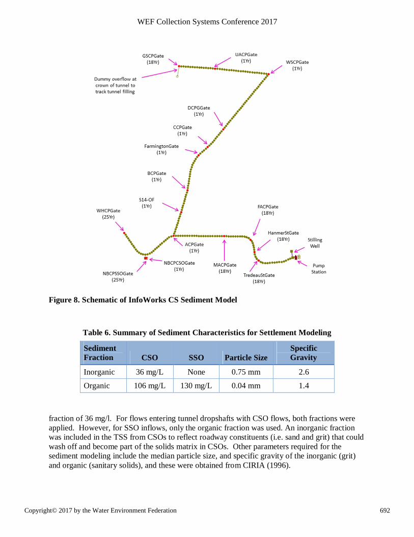
A schematic of the InfoWorks CS model is shown in Figure 8. Sediment transport in the North

Tunnel System may impact the South Tunnel System, and therefore the two tunnels were

analyzed as part of an integrated system. The InfoWorks model was based on the refined version

of the SWMM model with 5.49 m (18 feet) diameter tunnel reaches subdivided into 76 m (250

ft.) segments. Flow inputs to the tunnel were extracted from the SWMM model and were added

at the corresponding location in the InfoWorks model. The pump station at the HWPCF was

configured the same as in the SWMM model.

The InfoWorks software allows two sediment fractions to be simulated, such as organic (volatile

fraction) and inorganic (grit). Table 6 provides a summary of the sediment characteristics used

in the modeling. Information from previous studies indicated the average TSS were 142 mg/L.

Based on typical composition of untreated domestic wastewater (Metcalf & Eddy, 1991), the

TSS concentration of 142 mg/l was divided into an organic fraction of 106 mg/l and an inorganic



Figure 8. Schematic of InfoWorks CS Sediment Model

Table 6. Summary of Sediment Characteristics for Settlement Modeling

Sediment

Fraction CSO SSO Particle Size

Specific

Gravity

Inorganic 36 mg/L None 0.75 mm 2.6

Organic 106 mg/L 130 mg/L 0.04 mm 1.4

fraction of 36 mg/l. For flows entering tunnel dropshafts with CSO flows, both fractions were

applied. However, for SSO inflows, only the organic fraction was used. An inorganic fraction

was included in the TSS from CSOs to reflect roadway constituents (i.e. sand and grit) that could

wash off and become part of the solids matrix in CSOs. Other parameters required for the

sediment modeling include the median particle size, and specific gravity of the inorganic (grit)

and organic (sanitary solids), and these were obtained from CIRIA (1996).



Sensitivity Testing

Experience has shown that sediment modeling can be sensitive to the time step used in the

model. One of the ways that the results of sediment models can be assessed is by computing the

mass balance. This involves extracting from the simulation results the mass of TSS entering the

tunnel, the mass leaving the system through the pump station, and the mass that accumulates

(deposits) in the tunnel. Multiple model runs for the year 2002 were performed using both the

Ackers-White and Velikanov sediment modeling algorithms with various time steps. The mass

in for the year 2002 were the same for all of the model runs and was equal to 237,324 kg for the

organic fraction, and 80,222 kg for the inorganic fraction (total 317,546 kg). The model results

for the mass out, accumulation, and mass balance are summarized in Table 7.

As can be seen from the results in Table 7, a much greater fraction of the TSS is accumulating in

the tunnel for the Ackers-White sediment model than for the Velikanov. The model results

indicate the total mass balance errors generally decrease as the time step decreases for the

Ackers-White model, and increase for the Velikanov model. Generally, a lower time step results

in an improved mass balance. It is not known why the opposite occurred for the Velikanov

model. In this respect, the sensitivity results were inconclusive. Both sediment models were

used for the full analysis to provide an estimate of the uncertainty inherent in these types of

analyses.

Table 7. Results of Sediment Sensitivity Analysis

Sediment Model Results

Model simulations were conducted over the most recent 10 years for which flow data were

available (2002 – 2011), and the results are summarized in Table 8. Long term simulations are

warranted for sedimentation modeling as accumulation occurs gradually and erosion tends to

occur during larger storms.

It can be noted from the results in Table 8 that the net accumulation based on the Ackers-White

sediment model for the second 5-year period (years 6 through 10) was approximately half of the

accumulation for the first 5-year period, suggesting that the rate of sediment accumulation may

decrease. In contrast to the Ackers-White sediment model, the rate of sediment accumulation

based on the Velikanov sediment model is roughly the same for the two 5-year periods.

Time

Sediment Step Organic Inorganic Total Organic Inorganic Total Organic Inorganic Total

Model (sec) SF1 (kg) SF2 (kg) (kg) SF1 (kg) SF2 (kg) (kg) SF1 (%) SF2 (%) (%)

Ackers-White 60 158,118 368 158,486 42,767 70,250 113,018 15.4 12.0 14.5

Ackers-White 30 168,109 197 168,305 45,219 84,187 129,406 10.1 (5.2) 6.2

Ackers-White 10 175,786 221 176,007 49,271 73,312 122,583 5.2 8.3 6.0

Ackers-White 0.5 177,541 216 177,757 50,279 71,099 121,378 4.0 11.1 5.8

Velikanov 60 220,881 68,155 289,036 8,352 21,558 29,911 3.4 (11.8) (0.4)

Velikanov 30 225,928 65,282 291,210 6,697 18,734 25,431 2.0 (4.7) 0.3

Velikanov 10 226,541 47,376 273,916 8,222 28,424 36,646 1.1 5.5 2.2

Velikanov 0.5 227,227 47,113 274,341 7,942 28,704 36,646 0.9 5.5 2.1

Mass Out Accumulation Mass Balance



Table 8: Predicted Sediment Accumulation and Volume

Year Component Sediment Model Results

Ackers-White Velikanov

End of

Year 5

Mass In (kg) 2,478,900 2,478,900

Accumulation (kg) 651,900 288,500

Percentage of Mass Inflow Predicted to

Accumulate 26% 12%

Bulk Density (kg/m3) 1,595 1,662

Total Volume of Sediment (m3) 409 174

Mass Balance (%) 5.8 2.0

End of

Year 10

Mass In (kg) 5,006,300 5,006,300

Accumulation (kg) 973,800 586,700

Net Accumulation (kg) 321,900 298,200

Percentage of Mass Inflow Predicted to

Accumulate 19% 12%

Bulk Density (kg/m3) 1,640 1,650

Total Volume of Sediment (m3) 594 356

Mass Balance (%) 5.4 2.0

Assuming a porosity of 30%, the bulk density of the sediment was calculated for the various

simulations, and results are presented in Table 8. In general, the bulk density is on the order of

1,600 kg/m3 (99.7 lb/ft3). The mass balance errors were about 5.5 % for the Ackers-White

sediment model and 2% for the Velikanov sediment model. A positive mass balance error

indicates that more TSS entered the tunnel than accounted for by the mass existing at the pump

station and the mass that accumulated in the tunnel. Thus, the actual accumulations in the tunnel

could be marginally higher. However, the mass balance errors are considered within acceptable

limits for this type of analysis.

Figures 9 and 10 shows the sediment depth distribution in the South tunnel after 5 and 10 years

for the Ackers-White and Velikanov models, respectively. The sediment depth for the North

Tunnel is similar. In general, higher sediment accumulations are predicted to occur at the

downstream end of the South Tunnel. This follows logically since water will back up at this

location and provide the greatest opportunity for sediments to deposit. The sediment modeling

also predicts that the depth of sediment is lower just downstream of the S-19 and S-21 Gate

connection (refer to Figure 8). This is believed to occur because the North Tunnel connects at

this location, and the additional flow from the North Tunnel reduces the sediment deposition.

The maximum depth of sediment after 10-years is predicted to be less than about 0.3 meters (one

foot) for both the Ackers-White and Velikanov sediment models.



Figure 9. Predicted Sediment Depth for Ackers-White Sediment Model

Figure 10. Predicted Sediment Depth for Velikanov Sediment Model

0

10

20

30

40

50

60

70

80

90

0 1,000 2,000 3,000 4,000 5,000 6,000

Sed

imen

tD

epth

(cm

)

Distance from Upstream End of Tunnel (meters)

End of 5 Year

End of 10 Year

MACPGate

Franklin @

Standish

CTS3 S-19 &

S-21

Douglas and

PrestonHanmer

Tredeau

Pump

StationNTS

and

New

Britain

South Tunnel

0

10

20

30

40

50

60

70

80

90

0 1,000 2,000 3,000 4,000 5,000 6,000

Sed

imen

tD

epth

(cm

)

Distance from Upstream End of Tunnel (meters)

End of 5 Year

End of 10 Year

MACPGate

Franklin @

Standish

CTS3 S-19 &

S-21

Douglas and

PrestonHanmer

Tredeau

Pump

StationNTS

and

New

Britain

South Tunnel



As these results show, there is a lot of uncertainty with modeling of the sediment. The sediment

models produce results, and the challenge then becomes how to gain confidence in the

predictions. Some of the tools that were employed for the SCHST sediment modeling include

time step sensitivity testing, comparing results from two different sediment modeling algorithms,

and mass balance analyses. Based on these analyses, the general magnitude of the potential

sediment deposition was assessed and is believed to be reasonable.

CONCLUSIONS AND RECOMMENDATIONS

Hydraulic modeling is an important component in the planning, design, and optimization of deep

tunnel systems such as the SHCST. However, the model predictions have to be checked, and

challenged, in order to gain confidence in the results. Some of the ways this was done for the

SHCST include:

Compare Model Results for Different Time Steps

Numerical models can be unstable. In general, the longer the time step, the faster the model runs

and the more susceptible the results are to numerical instability. The instabilities may be

difficult to detect in a 54-year simulation. Time step sensitivity testing was performed on shorter

runs which indicated a 0.5 second time step produced the most accurate result.

Recommendation: An assessment of the time step should be made during model development

to confirm the model has time step independence, which means the model results are not

significantly affected by the selection of the time step used in the model.

Compare Volume Stored with Hand Calculations

The maximum volume of water stored in the tunnel was computed based on a mass balance

analysis using flow volume into the tunnel minus flow volume exiting the tunnel. The peak

hydraulic grade predicted by the model was then used to compute the volume of water stored in

the tunnel using hand calculations based on an inclined cylinder formula. The initial results

indicated a significant discrepancy (6 to 9 %) for the initial model configurations which utilized

relatively long tunnel segments. The discrepancy was reduced to 1.3 % by subdividing the

tunnel reaches into smaller segments.

Recommendation: Model results should be checked against hand calculations whenever

possible.

Recommendation: When applying SWMM for large diameter, relatively flat pipes, such as a

tunnel, care should be taken to avoid excessively long segments. If necessary, long pipes should

be subdivided.

Compare Design Storm and Continuous Simulation Results

Initial sizing of the tunnel was performed using design storms selected from the historical period

of record. Gate control and tunnel sizing for a 1-year storm should have, in theory, resulted in



about 54 overflows over a 54-year period. This was not the case for the SHCST because the

shape of the 1-year design storm used for the SHCST was not typical. The storm started out

slow and stopped, which allowed pumps to dewater the tunnel. When the storm picked up again,

it was essentially a new storm with a smaller volume than a 1-year design storm.

Recommendation. Confirm design storm simulation results with continuous simulations

whenever possible.

Use Predictive Control to Further Optimize Tunnel Performance

The 54-year period of record simulations resulted in too many CSOs in sensitive areas, which are

only allowed to overflow on average once every 18-years or twice in the 54-year period of

record. Iterative model simulations indicated that it was not possible to meet the CSO control

objectives with a pre-programmed gate control system without increasing the size of the tunnel.

However, many of the storms that resulted in CSOs in sensitive areas could have been predicted

days in advance by modern weather forecasts. As a result, human “Predictive Control” could be

used to further optimize the operation of the tunnel by closing the CSO gates earlier than the pre-

programmed set-points based the hydraulic model.

Recommendation: Don’t rely solely on model results for design and operations. Look for

opportunities to inject human thought, such as the application of Predictive Control, into the

process.

Check Sediment Calculations Carefully

Sediment calculations are inherently uncertain. Some of the tools that were employed for the

SHCST sediment modeling to check the results included time step sensitivity testing, comparing

results from two different sediment modeling algorithms, and mass balance analyses. The time

step testing established that a 0.5 second time step was appropriate. The results from the

different sediment modeling algorithms established the range of variability in these types of

analyses and the mass balance analyses provided a measure of the accuracy. Based on these

analyses, the general magnitude of the potential sediment deposition was assessed and was

determined to be minimal.

Recommendation: When performing sediment calculations, use multiple sediment models,

conduct time step testing, and check the mass balance.

It is hoped that the conclusions and recommendations presented above will be valuable to others

facing the design of similar tunnel systems to control wet weather overflows. Each tunnel

design should be carefully considered in terms of the site-specific overflow performance targets

and design criteria.

REFERENCES

AECOM in association with Black and Veatch, February 2013. South Hartford Conveyance &

Storage Tunnel, Hartford Connecticut. Final Basis of Design Report.



CIRIA, 1996, Report 141: Design of Sewers to Control Sediment Problems, Construction

Industry Research and Information Association, London.

Hartford MDC and CDM Smith, December 4, 2014. Long-Term Combined Sewer Overflow

Control Plan 2012 Update, The Metropolitan District, Hartford, Connecticut.

Metcalf & Eddy, Inc. 1991, Wastewater Engineering: Treatment, Disposal, and Reuse, Third

Edition, McGraw-Hill, Inc. New York.

Mignone, T. K, S. Craig, G. Heath, and J. Sullivan (2016), Functional Design for the South

Hartford CSO Storage Tunnel, Presented at Water Environment Federation Collection Systems

Specialty Conference, May 2, 2016.



Date post:	25-May-2018
Category:	Documents
Upload:	nguyenxuyen
View:	216 times
Download:	0 times

Mind Over Model: Optimization of Gate Closure for the ... Over Model: Optimization of Gate Closure...

Documents