MINERAL PRECIPITATION AND DEPOSITION IN COOLING SYSTEMS USING IMPAIRED WATERS: MECHANISMS, KINETICS, AND INHIBITION by Heng Li B.S.E., Tsinghua University, 1999 M.Phil., University of Hong Kong, 2001 M.S., University of Arizona, 2003 Submitted to the Graduate Faculty of Swanson School of Engineering in partial fulfillment of the requirements for the degree of Doctor of Philosophy University of Pittsburgh 2010
Transcript
MINERAL PRECIPITATION AND DEPOSITION IN COOLING SYSTEMS USING IMPAIRED WATERS: MECHANISMS, KINETICS, AND INHIBITION
by
Heng Li
B.S.E., Tsinghua University, 1999
M.Phil., University of Hong Kong, 2001
M.S., University of Arizona, 2003
Submitted to the Graduate Faculty of
Swanson School of Engineering in partial fulfillment
of the requirements for the degree of
Doctor of Philosophy
University of Pittsburgh
2010
ii
UNIVERSITY OF PITTSBURGH
SWANSON SCHOOL OF ENGINEERING
This dissertation was presented
by
Heng Li
It was defended on
July 27, 2010
and approved by
Radisav D. Vidic, Professor, Civil and Environmental Engineering Department
David A. Dzombak, Professor, Civil and Environmental Engineering Department (CMU)
Willie F. Harper, Jr., Associate Professor, Civil and Environmental Engineering Department
Di Gao, Assistant Professor, Chemical and Petroleum Engineering Department
Jason D. Monnell, Research Assistant Professor, Civil and Environmental Engineering
Department
Dissertation Director: Radisav D. Vidic, Professor
5.0 SCALING CONTROL IN ASH TRANSPORT/SETTLING POND WATER INTERNALLY USED IN COAL-FIRED POWER PLANT COOLING SYSTEMS........................................................................................................................................... 84
6.0 PREDICTING THE PH BEHAVIOR OF RECIRCULATING WATER IN COOLING TOWERS ................................................................................................... 103
7.0 INSIGHTS INTO MECHANISMS OF MINERAL SCALING INHIBITION BY POLYMALEIC ACID (PMA) .................................................................................... 119
8.0 ELECTROCHEMICAL IMPEDANCE SPECTROSCOPY (EIS) BASED CHARACTERIZATION OF MINERAL DEPOSITION FROM PRECIPITATION REACTIONS ................................................................................................................. 155
9.0 EXPANDED APPLICABILITY OF ELECTROCHEMICAL IMPEDANCE SPECTROSCOPY (EIS) FOR MINERAL DEPOSITION MONITORING UNDER BROAD WATER CHEMISTRIES ............................................................................. 183
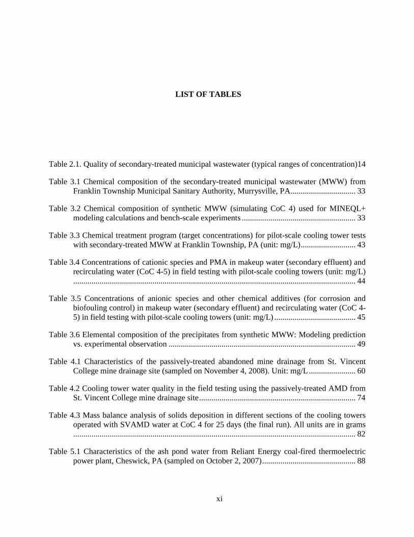
Table 2.1. Quality of secondary-treated municipal wastewater (typical ranges of concentration) 14
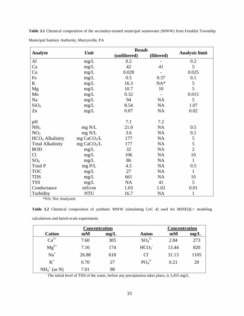
Table 3.1 Chemical composition of the secondary-treated municipal wastewater (MWW) from Franklin Township Municipal Sanitary Authority, Murrysville, PA ................................ 33
Table 3.2 Chemical composition of synthetic MWW (simulating CoC 4) used for MINEQL+ modeling calculations and bench-scale experiments ........................................................ 33
Table 3.3 Chemical treatment program (target concentrations) for pilot-scale cooling tower tests with secondary-treated MWW at Franklin Township, PA (unit: mg/L) ........................... 43
Table 3.4 Concentrations of cationic species and PMA in makeup water (secondary effluent) and recirculating water (CoC 4-5) in field testing with pilot-scale cooling towers (unit: mg/L)
Table 3.5 Concentrations of anionic species and other chemical additives (for corrosion and biofouling control) in makeup water (secondary effluent) and recirculating water (CoC 4-5) in field testing with pilot-scale cooling towers (unit: mg/L) ........................................ 45
Table 3.6 Elemental composition of the precipitates from synthetic MWW: Modeling prediction vs. experimental observation ............................................................................................ 49
Table 4.1 Characteristics of the passively-treated abandoned mine drainage from St. Vincent College mine drainage site (sampled on November 4, 2008). Unit: mg/L ....................... 60
Table 4.2 Cooling tower water quality in the field testing using the passively-treated AMD from St. Vincent College mine drainage site ............................................................................. 74
Table 4.3 Mass balance analysis of solids deposition in different sections of the cooling towers operated with SVAMD water at CoC 4 for 25 days (the final run). All units are in grams
Table 5.1 Characteristics of the ash pond water from Reliant Energy coal-fired thermoelectric power plant, Cheswick, PA (sampled on October 2, 2007) .............................................. 88
xii
Table 5.2 Chemical composition of synthetic ash pond water effluent (representing 4 cycles of concentration) ................................................................................................................... 98
Table 6.1 Chemical constituents of the modeling water representing secondary-treated municipal wastewater used for equilibrium calculations ................................................................. 106
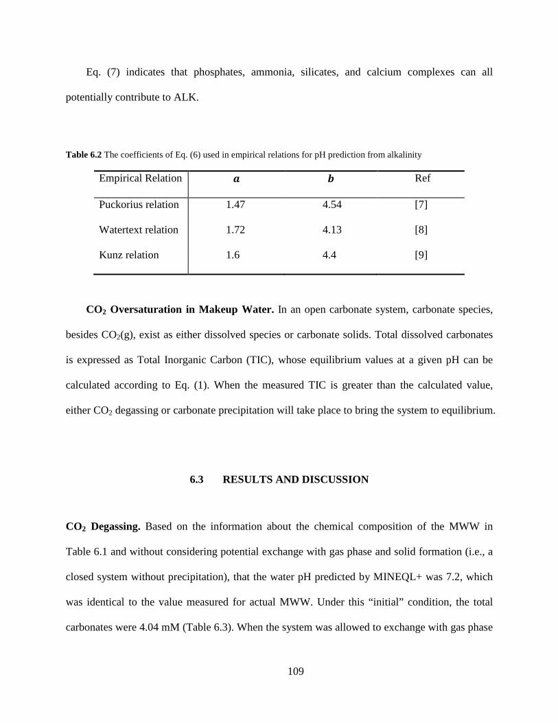
Table 6.2 The coefficients of Eq. (6) used in empirical relations for pH prediction from alkalinity ......................................................................................................................................... 109
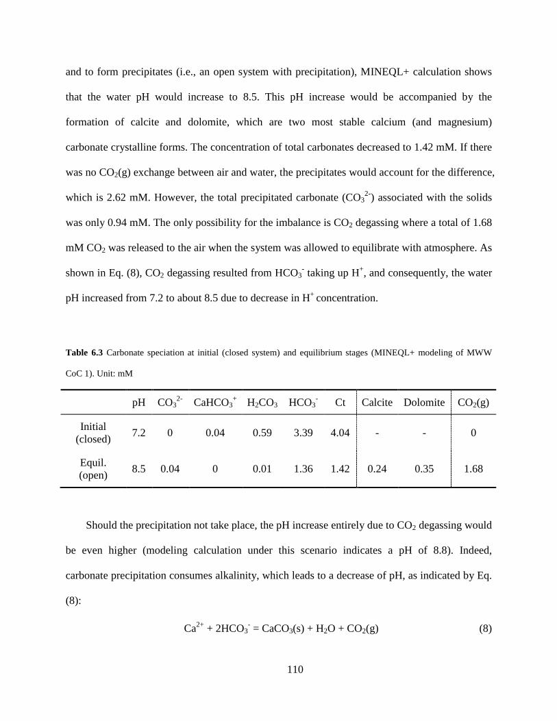
Table 6.3 Carbonate speciation at initial (closed system) and equilibrium stages (MINEQL+ modeling of MWW CoC 1). Unit: mM .......................................................................... 110
Table 7.1 Critical cluster formation and associated energy barrier ............................................ 126
Table 7.2 Surface free energies of minerals ................................................................................ 131
Table 7.3 Initial concentrations of the chemical constituents in bulk solutions for mineral precipitation retardation studies with PMA (unit: mM) ................................................. 136
Table 7.4 Concentrations of cations tested for their association/complexation with PMA ........ 137
Table 7.5 Amount (weight) of stainless steel wire used in each adsorption isotherm test with different amount of PMA ................................................................................................ 138
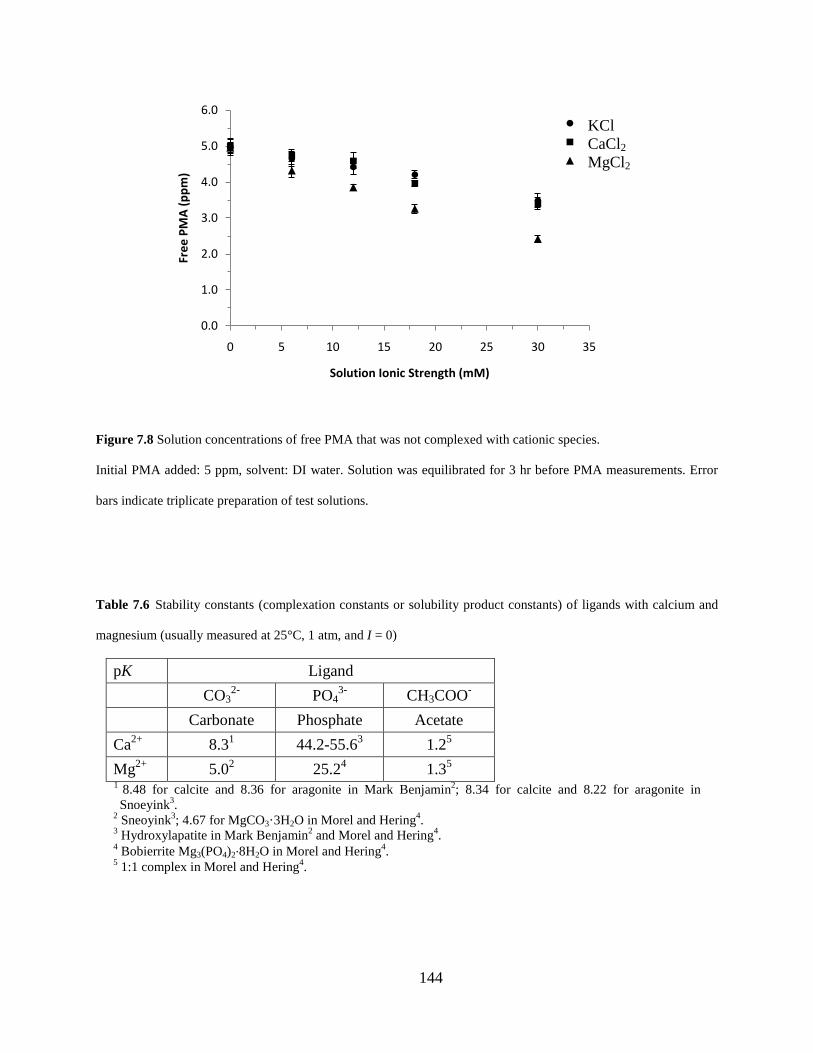
Table 7.6 Stability constants (complexation constants or solubility product constants) of ligands with calcium and magnesium (usually measured at 25°C, 1 atm, and I = 0) ................. 144
Table 7.7 Amount (weight) of stainless steel wire used in each adsorption isotherm test with different amount of PMA ................................................................................................ 147
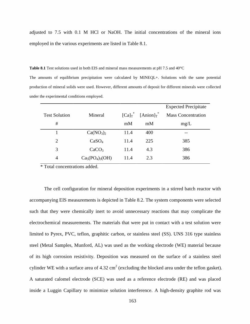
Table 8.1 Test solutions used in both EIS and mineral mass measurements at pH 7.5 and 40°C ......................................................................................................................................... 163
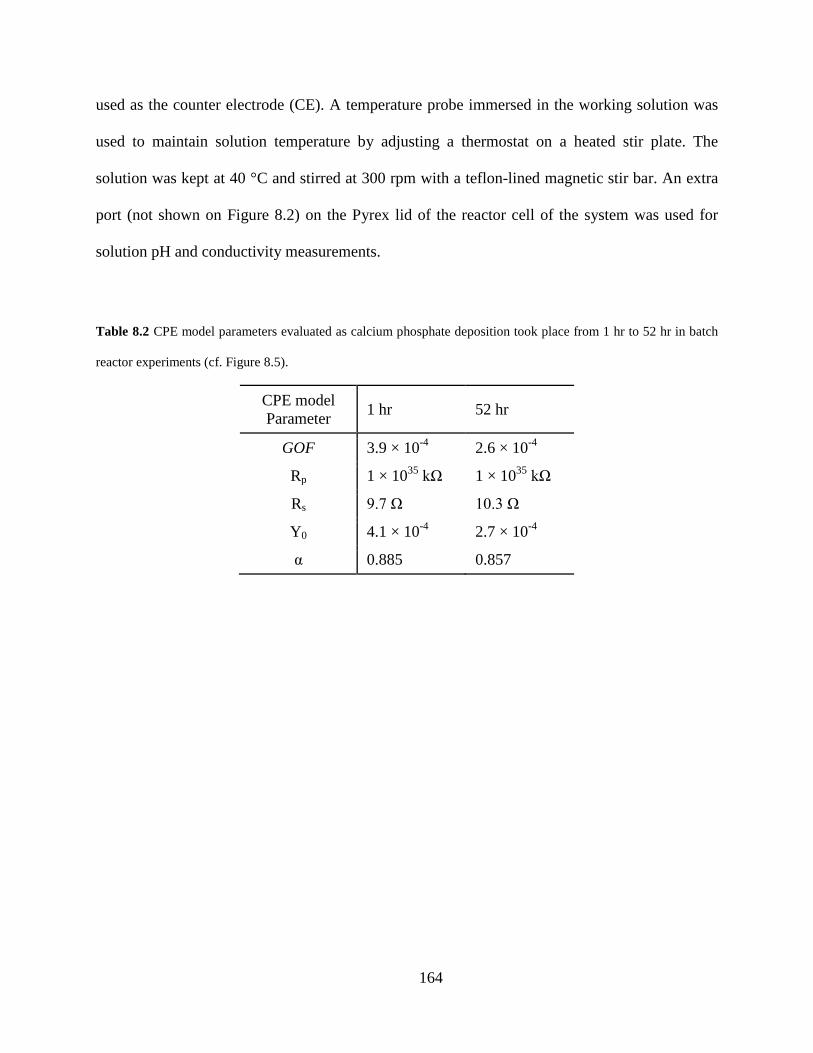
Table 8.2 CPE model parameters evaluated as calcium phosphate deposition took place from 1 hr to 52 hr in batch reactor experiments (cf. Figure 8.5). ................................................... 164
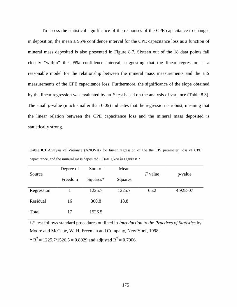
Table 8.3 Analysis of Variance (ANOVA) for linear regression of the the EIS parameter, loss of CPE capacitance, and the mineral mass deposited ǂ. Data given in Figure 8.7 .............. 175
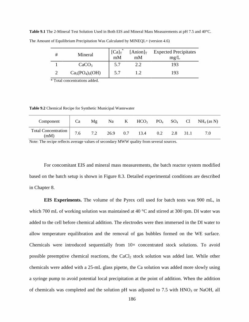
Table 9.1 The 2-Mineral Test Solution Used in Both EIS and Mineral Mass Measurements at pH 7.5 and 40°C. .................................................................................................................. 186
Table 9.2 Chemical Recipe for Synthetic Municipal Wastewater .............................................. 186
xiii
LIST OF FIGURES
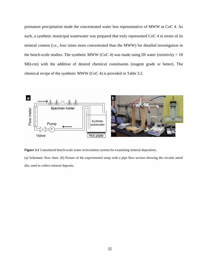
Figure 3.1 Customized bench-scale water recirculation system for examining mineral deposition.. ........................................................................................................................ 32
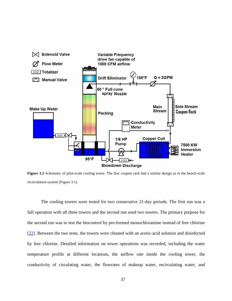
Figure 3.2 Schematic of pilot-scale cooling tower. The disc coupon rack had a similar design as in the bench-scale recirculation system (Figure 3.1). ....................................................... 37
Figure 3.3 Scaling behavior of a synthetic municipal wastewater (CoC 4) in bench-scale tests with inhibitors at different dosing (40°C). ........................................................................ 39
Figure 3.4 Influence of ammonia and phosphate on scaling control in bench tests with a synthetic MWW at CoC 4 (40°C) .................................................................................................... 40
Figure 3.5 Interference of chlorine-based biocides on scaling control in bench tests with a synthetic MWW at CoC 4 (40°C). .................................................................................... 41
Figure 3.6 Interference of chlorine biocides with PMA on scaling control in bench tests with a synthetic MWW at CoC 4 (40°C). .................................................................................... 41
Figure 3.7 Deposit mass measurements in the pilot-scale cooling tower tests using secondary-treated MWW. ................................................................................................................... 47
Figure 3.8 SEM image (left) and quantitative 1D EDS analysis (right) of the deposits collected on a stainless steel disc immersed in synthetic MWW in bench-scale water recirculating system. .............................................................................................................................. 51
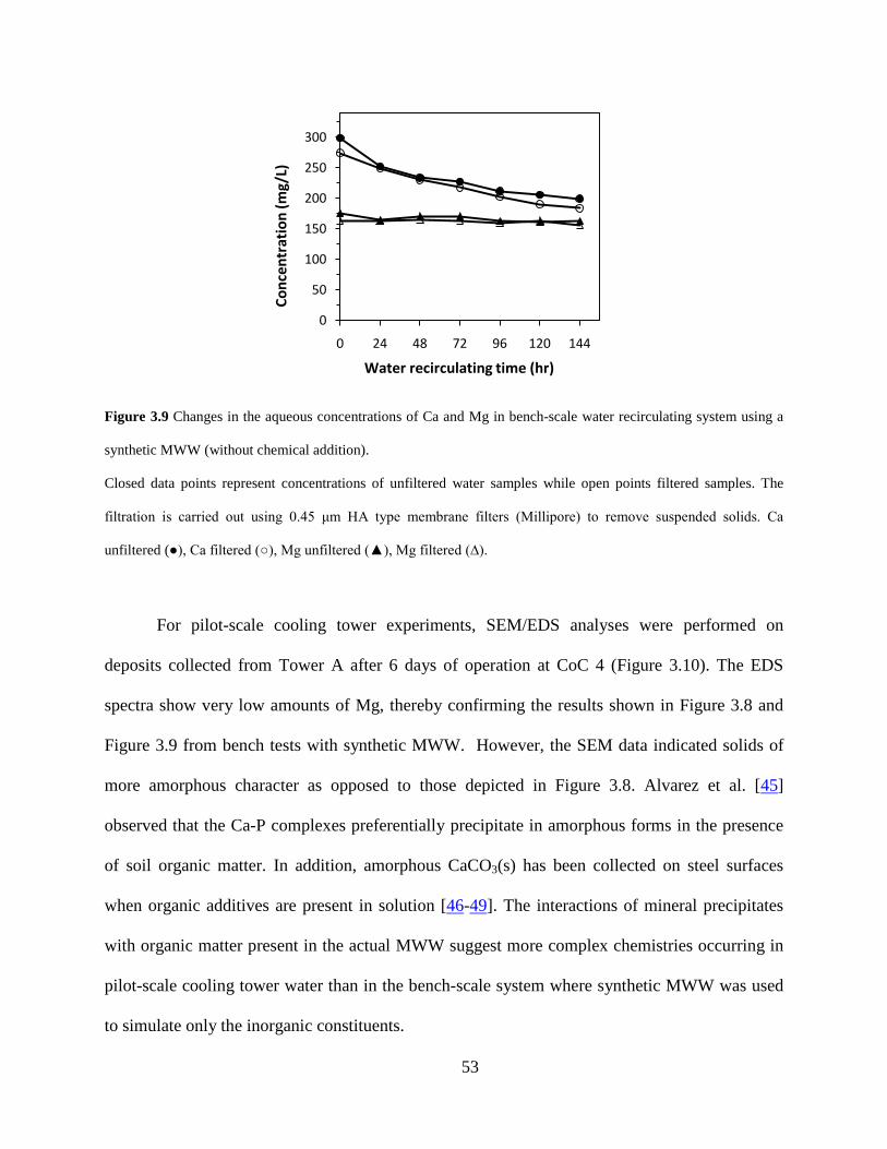
Figure 3.9 Changes in the aqueous concentrations of Ca and Mg in bench-scale water recirculating system using a synthetic MWW (without chemical addition). .................... 53
Figure 3.10 SEM image and the elemental composition of the solid deposits collected on a stainless steel disc immersed in the secondary-treated MWW in the pilot-scale cooling tower (Tower A) operated at CoC 4. ................................................................................ 54
Figure 4.1 Bench-scale water recirculating system with inserted stainless steel circular disc specimens for scale collection and subsequent mass gain measurement. ......................... 63
xiv
Figure 4.2 Modeling results of LSI (left) and RSI (right) for both open and closed to air cases without solids precipitation. .............................................................................................. 67
Figure 4.3 Predicted solid precipitation from the St. Vincent College Abandoned Mine Drainage calculated by MINEQL+. ................................................................................................. 68
Figure 4.4 Predicted solution pH at different CoC under four different operation scenarios (open or closed to air; with and without solid precipitation). ..................................................... 68
Figure 4.5 Correlation of concentration cycles determined by water volume reduction and conductivity measurements. .............................................................................................. 70
Figure 4.6 Coupon mass gain measurements for bench-scale water recirculating systems operated with the SVAMD (the water was stored in lab for a week prior to test). Recirculation conditions: 3 GPM, 40°C, pH 8.5. .................................................................................... 71
Figure 4.7 Effectiveness of different antiscalants in beaker tests at 40-45°C. ............................. 72
Figure 4.8 Coupon mass gain measurement for bench-scale water recirculating systems fed with the SVAMD water. ........................................................................................................... 73
Figure 4.9 Mass gain measurements in pilot-scale cooling towers operated with SVAMD water at FTMSA site. .................................................................................................................. 77
Figure 4.10 Total PMA (left panel) and dissolved (aqueous) PMA (right panel) concentrations in the recirculating water of the cooling towers as measured after daily addition of PMA (with 0.5 hr delay). ............................................................................................................ 79
Figure 4.11 Turbidity of the makeup water and the recirculating water in the cooling towers during the CoC 4 operation. .............................................................................................. 81
Figure 5.1 Bench-scale water recirculating system with inserted stainless steel circular disc specimens for scale collection and subsequent mass gain measurement. ......................... 90
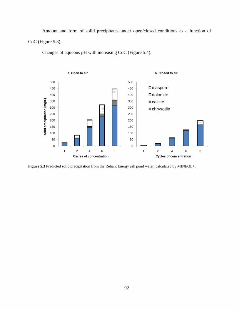
Figure 5.2 Modeling results of LSI (left) and RSI (right) for both open and closed to air cases, Reliant Energy ash pond water. ........................................................................................ 91
Figure 5.3 Predicted solid precipitation from the Reliant Energy ash pond water, calculated by MINEQL+. ........................................................................................................................ 92
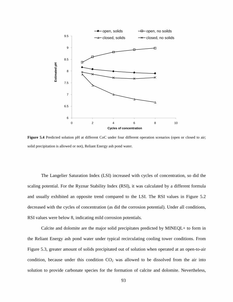
Figure 5.4 Predicted solution pH at different CoC under four different operation scenarios (open or closed to air; solid precipitation is allowed or not), Reliant Energy ash pond water. .. 93
Figure 5.5 Scaling behavior of the Reliant Energy ash pond effluent in bench-scale water recirculating tests: effect of cycles of concentration (CoC). ............................................. 95
Figure 5.6 Changes in solution TDS as a function of CoC for Reliant Energy ash pond water. .. 95
xv
Figure 5.7 Scaling behavior of synthetic ash pond effluent in bench-scale tests: effectiveness of different antiscalants at CoC 4. ......................................................................................... 97
Figure 5.8 Changes in the aqueous concentrations of calcium and magnesium in the synthetic ash pond water in bench-scale tests. ........................................................................................ 99
Figure 5.9 Aqueous concentrations of calcium and magnesium in the synthetic ash pond water with antiscaling control by PMA (left) or PBTC (right). ................................................ 100
Figure 5.10 The stabilization of aqueous concentrations of calcium and magnesium in the synthetic ash pond water under scaling control by PMA-PBTC (left) is in agreement with the relatively constant PMA concentration in the water (right). ..................................... 101
Figure 6.1 pH increase due to CO2 degassing by aeration experiment using secondary-treated MWW. Error bars indicate the measurement ranges. ..................................................... 111
Figure 6.2 Total ammonia concentration in secondary MWW in beaker stripping test in the lab. Water temperature was raised from 23 to 40°C at 2500 min. ......................................... 112
Figure 6.3 Correlation between pH and ALK. The open circles are modeling results of open equilibrium conditions. ................................................................................................... 113
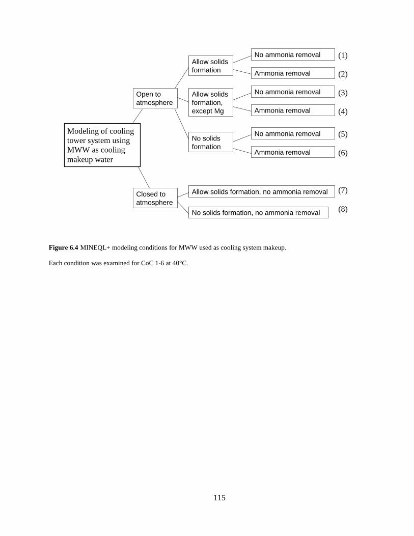
Figure 6.4 MINEQL+ modeling conditions for MWW used as cooling system makeup. ......... 115
Figure 6.5 Modeling of pH as a function of CoC under different operational conditions. ......... 116
Figure 7.1 Simplified schematic of the physical chemical processes of mineral scaling and scaling control by chemical additives. ............................................................................ 122
Figure 7.2 Energetics of mineral nucleation. .............................................................................. 127
Figure 7.3 Repeating unit of polymaleic acid. ............................................................................ 134
Figure 7.4 Effect of PMA addition on the precipitation reaction as measured by solution conductivity changes over time. ..................................................................................... 135
Figure 7.5 Solution conductivity changes over time in the absence and presence of PMA (5 ppm, added at time 0). .............................................................................................................. 140
Figure 7.6 SEM images of the precipitated mineral particles collected under different PMA treatment. ........................................................................................................................ 140
Figure 7.7 Elemental composition of the precipitated mineral particles collected after different PMA treatment. ............................................................................................................... 142
Figure 7.8 Solution concentrations of free PMA that was not complexed with cationic species. ......................................................................................................................................... 144
xvi
Figure 7.9 Suspension turbidity changes over time in the presence and absence of PMA (5 ppm, added at time 0). .............................................................................................................. 146
Figure 7.10 Solution PMA concentration in batch reactors made of different materials. .......... 147
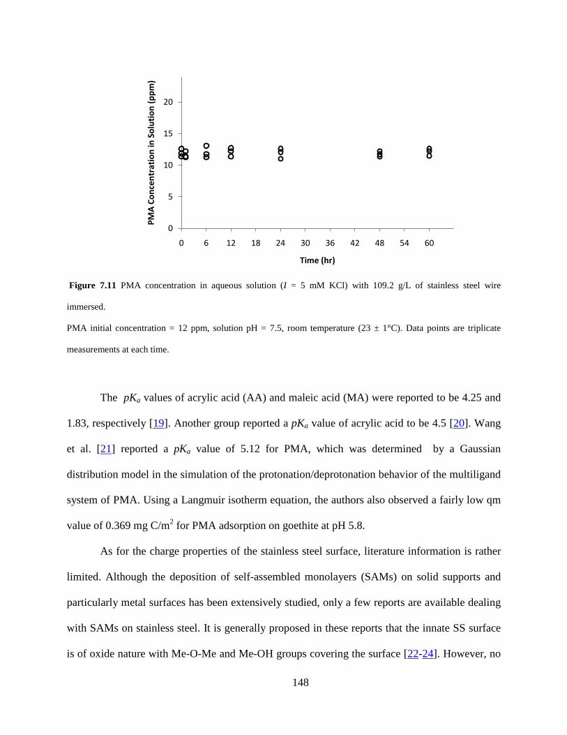
Figure 7.11 PMA concentration in aqueous solution (I = 5 mM KCl) with 109.2 g/L of stainless steel wire immersed. ....................................................................................................... 148
Figure 7.12 PMA equilibrium concentration as a function of initial concentration in aqueous solution (I = 5 mM KCl) containing stainless steel wire (Table 7.12). .......................... 149
Figure 7.13 Variation in particle size distribution of the mineral suspension with different PMA treatment. ........................................................................................................................ 150
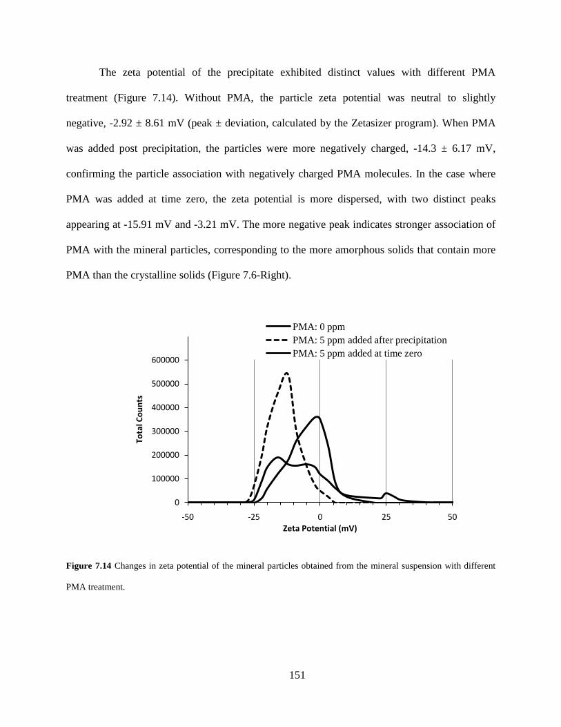
Figure 7.14 Changes in zeta potential of the mineral particles obtained from the mineral suspension with different PMA treatment. ..................................................................... 151
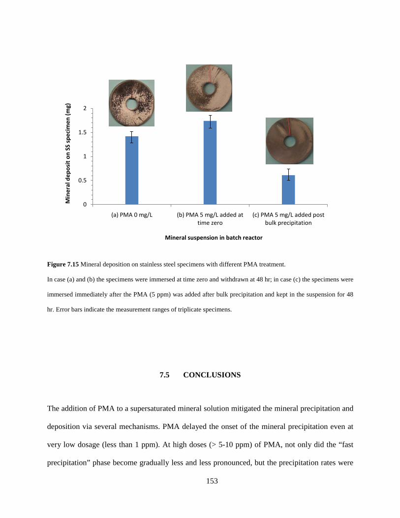
Figure 7.15 Mineral deposition on stainless steel specimens with different PMA treatment. .... 153
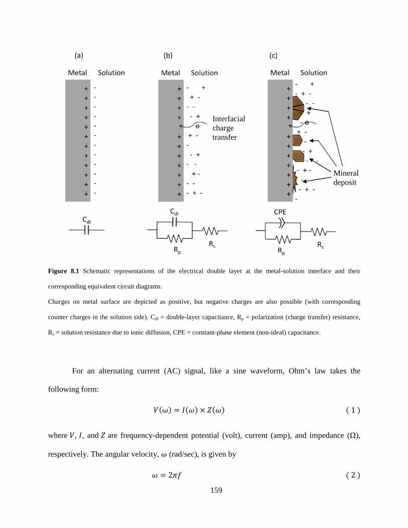
Figure 8.1 Schematic representations of the electrical double layer at the metal-solution interface and their corresponding equivalent circuit diagrams. ..................................................... 159
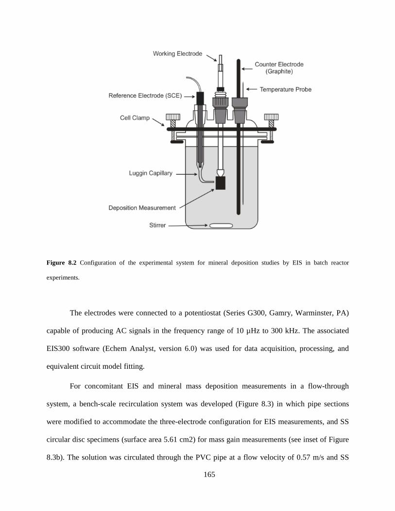
Figure 8.2 Configuration of the experimental system for mineral deposition studies by EIS in batch reactor experiments. .............................................................................................. 165
Figure 8.3 Customized bench-scale water recirculation system for simultaneous measurements of EIS and mineral mass deposited. .................................................................................... 166
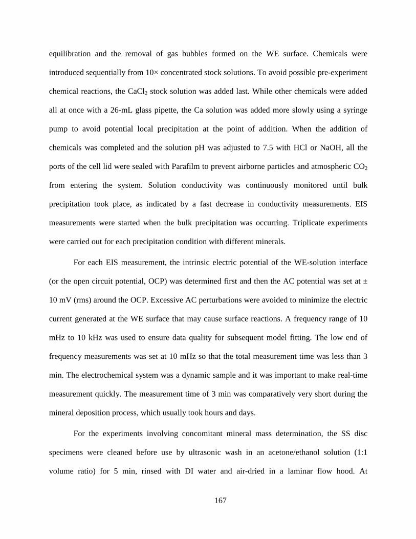
Figure 8.4 Representative EIS measurement on the stainless steel WE surface in the batch reactor system when the Ca-P deposition took place for 1 hr. .................................................... 169
Figure 8.5 EIS measurements in batch reactor tests with test solution #4 at two different times. ......................................................................................................................................... 171
Figure 8.6 Decrease of CPE capacitance 𝒀𝟎 due to calcium phosphate deposition on the stainless steel working electrode in batch reactor tests with test solution #4. ............................... 172
Figure 8.7 Loss of CPE capacitance (%) vs. mineral mass deposited (mg) for test solution #4. 174
Figure 8.8 Reduction of CPE capacitance normalized to mineral mass deposited per unit surface area for different mineral deposits studied. ..................................................................... 177
Figure 8.9 Analysis of the frequency-dependent accuracies of EIS measurements. .................. 179
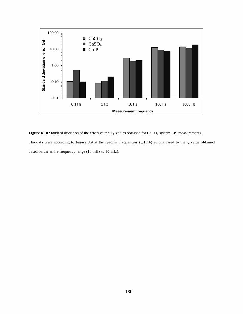
Figure 8.10 Standard deviation of the errors of the 𝒀𝟎 values obtained for CaCO3 system EIS measurements. ................................................................................................................. 180
Figure 9.1 Scatter plot (left) and residuals plot (right) of the data from simultaneous EIS and mineral mass measurements (CaCO3 + CaP). ................................................................ 189
xvii
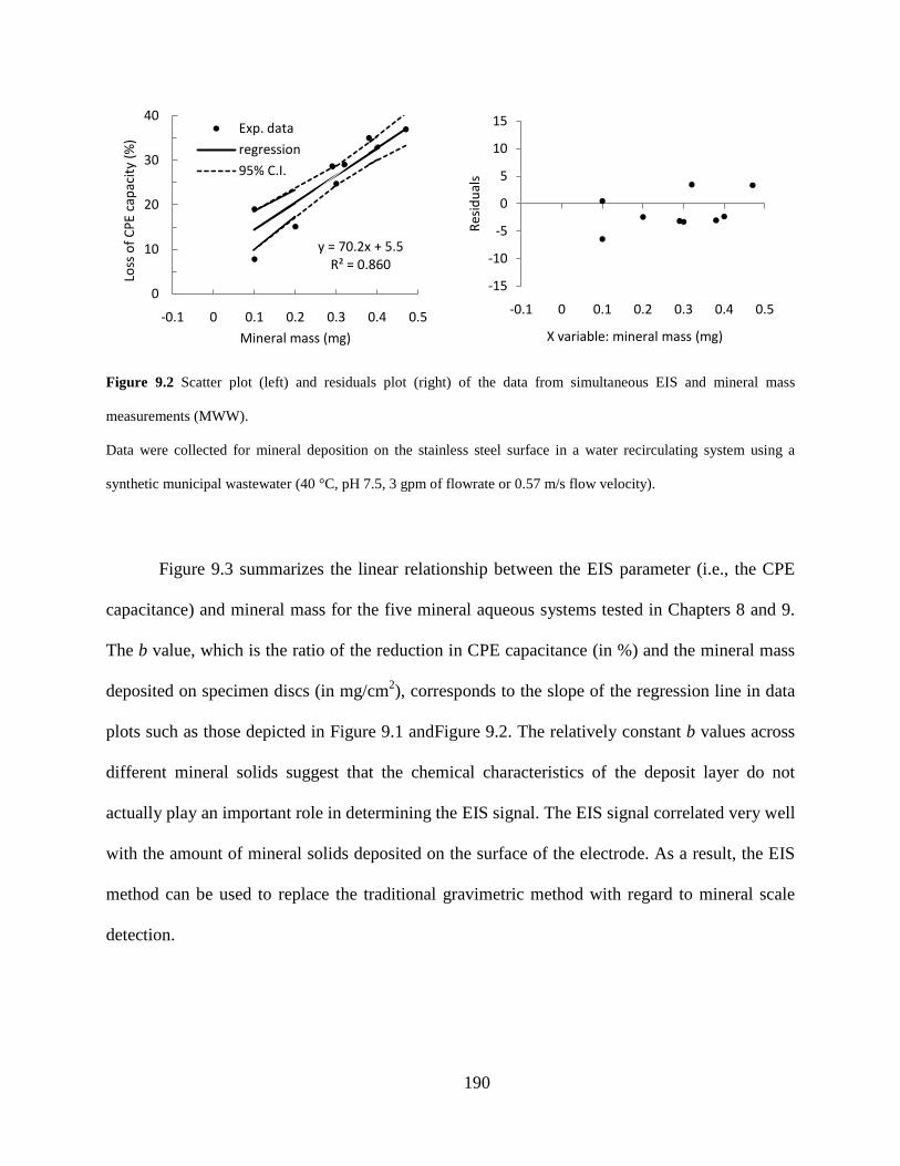
Figure 9.2 Scatter plot (left) and residuals plot (right) of the data from simultaneous EIS and mineral mass measurements (MWW). ............................................................................ 190
Figure 9.3 CPE capacitance vs. mineral mass deposited: the ratio (b value) of reduction of the CPE capacitance and the mineral mass deposited per surface area for different minerals.
Figure 9.4 EIS at the stainless steel WE surface before and after PMA addition (5 ppm) in aqueous solution. ............................................................................................................. 192
Figure 9.5 EIS at the stainless steel WE surface with or without chlorine biocides. .................. 194
xviii
ACRONYMS AND NOMENCLATURE
AAS Atomic Absorption Spectroscopy
AC Alternating Current
ALK Alkalinity (as CaCO3)
AMD Abandoned Mine Drainage
ANOVA Analysis Of Variance
APW Ash-settling Pond Water
atm Atmosphere (air pressure)
BGD Billion Gallons per Day
BOD Biological Oxygen Demand
CCS/CCR Carbon Capture and Sequestration/Recovery
CE Counter Electrode
CFU Colony Forming Unit
C.I. Confidence Interval
CoC Cycles of Concentration
COD Chemical Oxygen Demand
CPE Constant-Phase Element
DBPs Disinfection Byproducts
xix
DC Direct Current
DLVO Theory Derjaguin, Landau, Verwey, and Overbeek Theory
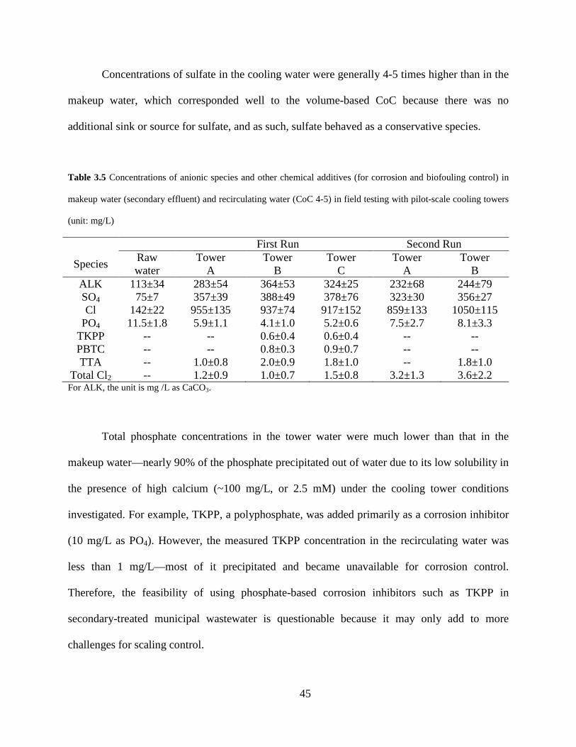
Filterable -- -- 4.3±1.3 9.7±2.1 -- 4.5±1.3 Data are mean values ± 1 sd. Sample size for raw water n = 7. Samples for recirculating water in the cooling towers were from day 4 to day 24 during the tower operation (sample size for tower A: 10, tower B: 10, tower C: 11).
Concentrations of chloride in the cooling water were typically 6-7 times higher than in
the makeup water. This ratio is higher than the expected ratio based on the water volume
reduction (i.e., CoC 4-5). The extra chloride of some 350 mg/L (estimation based on Table 3.5)
in the recirculating water came from the addition of chlorine biocides (either free chlorine for the
first run or monochloramine for the second run).
45
Concentrations of sulfate in the cooling water were generally 4-5 times higher than in the
makeup water, which corresponded well to the volume-based CoC because there was no
additional sink or source for sulfate, and as such, sulfate behaved as a conservative species.
Table 3.5 Concentrations of anionic species and other chemical additives (for corrosion and biofouling control) in
makeup water (secondary effluent) and recirculating water (CoC 4-5) in field testing with pilot-scale cooling towers
For pilot-scale cooling tower experiments, SEM/EDS analyses were performed on
deposits collected from Tower A after 6 days of operation at CoC 4 (Figure 3.10). The EDS
spectra show very low amounts of Mg, thereby confirming the results shown in Figure 3.8 and
Figure 3.9 from bench tests with synthetic MWW. However, the SEM data indicated solids of
more amorphous character as opposed to those depicted in Figure 3.8. Alvarez et al. [45]
observed that the Ca-P complexes preferentially precipitate in amorphous forms in the presence
of soil organic matter. In addition, amorphous CaCO3(s) has been collected on steel surfaces
when organic additives are present in solution [46-49]. The interactions of mineral precipitates
with organic matter present in the actual MWW suggest more complex chemistries occurring in
pilot-scale cooling tower water than in the bench-scale system where synthetic MWW was used
to simulate only the inorganic constituents.
0
50
100
150
200
250
300
0 24 48 72 96 120 144
Conc
entr
atio
n (m
g/L)
Water recirculating time (hr)
54
Figure 3.10 SEM image and the elemental composition of the solid deposits collected on a stainless steel disc
immersed in the secondary-treated MWW in the pilot-scale cooling tower (Tower A) operated at CoC 4.
EDS scan was performed on the area outlined by the square box on the SEM image.
The EDS analyses conducted on the solids collected from pilot experiments indicate that
the deposits consisted primarily of calcium carbonates and phosphates, which is in qualitative
agreement with the revised model predictions discussed earlier. However, the quantity of
phosphates appears to be greatly enriched when compared to that in the deposits collected from
the bench-sale studies using synthetic MWW. This is likely because of the higher P
concentration in the actual MWW (i.e., 12 mg/L vs. 5 mg/L in the synthetic water). In addition,
P-containing chemicals, in the form of TKPP (10 mg/L) and PBTC (5 mg/L), were also added to
the cooling towers for corrosion/scaling control. Chemical analyses indicated that these added
55
phosphates quickly became undetectable in the liquid phase, suggesting their precipitation that
further contributed to the relatively high P signal in the EDS spectra (Figure 3.10).
3.4 CONCLUSIONS
This study demonstrates the feasibility and challenges of using secondary-treated municipal
wastewater as an alternative cooling system makeup water to replace freshwater. The scaling
behavior and control of it in recirculating cooling systems was evaluated. Based on the results
from bench-scale experiments performed in this study, it was determined that commonly used
polymer-based scaling inhibitors can be effective in controlling potentially severe scaling when
using this impaired water as makeup in recirculating cooling systems. PMA worked very well at
scaling inhibition in the absence of chlorine disinfectants but only partially effective in the
presence of chlorine. Ammonia present in the wastewater could suppress the aggressiveness of
free chlorine on PMA. Pre-formed monochloramine was found to be less aggressive than free
chlorine, while still being an effective biocide. Pilot-scale cooling tower experiments suggested
that mineral scaling control by PMA was much more challenging due to biofouling.
Overall, for scaling control of MWW that is concentrated to CoC 4 in recirculating
cooling systems, 1) PMA can be applied at 10 mg/L level for effective mineral scaling inhibition
in the absence of biofouling, 2) monochloramine is better suited as biocide than free chlorine
because of the reduced impact of monochloramine on antiscaling programs, and 3) phosphorous
based scaling and corrosion inhibitors are not appropriate due to their precipitation with Ca.
56
4.0 SCALING CONTROL FOR REUSE OF PASSIVELY-TREATED ABANDONED
MINE DRAINAGE IN RECIRCULATING COOLING SYSTEMS
In coal mining regions where substantial coal-based power generation takes place, significant
quantities of abandoned mine water that exists in mine voids represent a potential for use as a
stable, large volume supply of cooling water. Reusing passively-treated abandoned mine
drainage (AMD) can avoid surface water contamination that can otherwise occur due to the
overflow of the AMD from mine pools, which is usually acidic and contains high concentrations
of metals, especially iron and manganese. However, since using AMD for cooling is not widely
practiced, knowledge about the proper control of scaling issues in cooling systems using AMD is
limited. The use of AMD is predicated on being pre-treated with aeration/settling ponds to
remove Fe/Mn and suspended solids. In this study, the scaling behaviors of passively-treated
AMD and scaling mitigation in cooling water systems were investigated through laboratory and
pilot-scale experiments. Bench-scale recirculating systems and three pilot-scale cooling towers
were employed for testing various chemical control schemes for scaling control in AMD. The
tests were conducted under conditions of temperature, flow velocities, and water constituent
concentrations similar to those in a recirculating cooling water system. The effectiveness of
chemical treatment strategies in inhibiting mineral scaling was evaluated through exposure and
monitoring of specially designed disc specimens in extended experimental tests. Polymaleic acid
(PMA) effectively decreased the settling of suspended solids and rendered the solids less prone
57
to deposition onto the surfaces immersed in the pipe flow sections. In the absence of PMA,
significant amounts of solids settled in the sumps of pilot-scale cooling towers where flow
velocity was minimal. The PVC and stainless steel surfaces exhibited different affinities for
scaling; PVC was determined to yield increased deposition in bench-scale recirculation systems.
The observation implies that varied severity of scaling problems can take place in recirculating
sections of a cooling system made of different materials, which was also observed in the pilot-
scale cooling towers using the same type of passively-treated AMD.
4.1 INTRODUCTION
Abandoned mine drainage (AMD) refers to the release of the contaminated groundwater
produced by dissolution of sulfide minerals (especially pyrite FeS2(s)) and commonly found in
the areas adjacent to abandoned mine sites [1]. AMD is characterized by low pH, high content of
iron hydroxides, as well as elevated levels of heavy metals [2]. These characteristics are
manifested in streams impacted by AMD through sediment color ranging from red to orange or
yellow due to iron precipitation, and significant endangerment of aquatic and benthic life [3].
Coal mining produces the bulk of AMD. This is especially true in Pennsylvania where
more than 25% of the nation’s total coal output was produced over the past 200 years [4]. As
such, AMD has been a major water-pollution problem in Pennsylvania where over 3,000 miles of
streams and associated ground waters have been contaminated [4]. Other areas in the US with
large volumes of AMD include the other Appalachian coal-producing states and the Illinois-
Indiana coal mining region [5]. AMD is also generated in the hard-rock mining areas of the
western US, although such water was not examined in this study.
58
Given the large quantity of AMD available, it may be possible to use it for cooling
purposes in areas of the US where freshwater shortages occur frequently [6, 7]. This practice
may significantly impact water conservation as consumptive withdrawal of freshwater by
thermoelectric power generation cooling water systems can contribute significantly to the water
shortage problem in some areas. In the US, thermoelectric power generation consumed 3.3 BGD
of freshwater in 1995, mainly through evaporative loss from cooling towers [8].
Waters of impaired quality, such as AMD, are of increasing interest as alternative sources
to freshwater for thermoelectric power plant recirculating cooling water systems. The AMD
represents significant quantities of possible cooling system makeup water in coal mining regions
where substantial coal-based power generation takes place [9, 10]. It was estimated that there is
approximately 250 billion gallons of mine pool volume in West Virginia and Pennsylvania [9].
In addition to supplementing withdrawal of surface water for cooling, other benefits of reusing
mine pool water in power plants are the prevention of AMD-related surface water contamination,
and additional flexibility in siting new power plants. Although active pretreatment might be
necessary to raise the water quality of AMD to allow reuse (treatments typically raise pH, reduce
metal concentration and total dissolved solids), the development and successful implementation
of passive treatment systems makes it promising to access AMD with better quality [11, 12].
Further, AMD chemical compositions often evolve over time to become less acidic and can
approach neutral pH in many cases, as well as have lower loads of dissolved solids over time
[13]. Such AMD can be treated with temporary retention in ponds to allow oxidation and iron
precipitation. Passively-treated, near-neutral pH AMD waters are good candidates for use in
power plant cooling systems. Indeed, there is already some experience with operating their
cooling systems totally or partially with treated AMD in Pennsylvania [14].
59
However, mineral precipitation and subsequent surface scaling remains one of the main
challenges for AMD reuse in recirculating cooling water systems. Up to date, knowledge in the
literature concerning mineral scaling in cooling systems caused by AMD is limited due to the
fact that using AMD as cooling tower makeup is not widely practiced.
The goal of this study was to evaluate the technical feasibility of reusing AMD in power
plant cooling tower systems. Specifically, the objectives of this study were to 1) simulate scale
formation under cooling tower operation conditions at different cycles of concentration via
chemical equilibrium modeling, 2) test the effectiveness of different chemical treatment
programs on scaling inhibition in bench-scale water recirculating systems, and 3) determine the
viability of using AMD as cooling water makeup through testing in a pilot-scale cooling tower
system.
4.2 MATERIALS AND METHODS
4.2.1 Passively-treated AMD characterization and preparation for laboratory and field
testing
Passively-treated AMD from the St. Vincent College mine drainage site (Latrobe, PA) was
chosen for testing in laboratory experiments and in pilot-scale cooling towers. Passive treatment
at the St. Vincent site is accomplished through a system of constructed wetlands to reduce iron
content. A total of 7,000 gallon of the AMD for use as makeup water in tests with pilot-scale
cooling towers was collected and transported to our test site at the Franklin Township Municipal
Sanitary Authority (Murrysville, PA) by a steel tanker truck on September 30, 2008. The AMD
60
was transferred to a covered and lined steel roll-off container stored outside at ambient
temperature and was used as needed.
Table 4.1 Characteristics of the passively-treated abandoned mine drainage from St. Vincent College mine drainage
site (sampled on November 4, 2008). Unit: mg/L
Analyte Result Reporting limit Al ND 0.4 Ca 228 10 Cu ND 0.05 Fe ND 0.2 K 5.21 B 10 Mg 61.8 10 Mn 0.172 0.03 Na 96.4 10 SiO2 14.9 2.14 Zn 0.0281 B 0.04
pH 7.8 NH3-N 0.34 J 0.1 Bicarbonate Alkalinity 117 J 5 BOD ND 2 Cl 56.1 1 NO3-N 0.32 0.05 SO4 656 J 25 Total P 0.056 B 0.1 Total Alkalinity 117 J 5 TOC 1.7 1 TDS 991 10 TSS ND 4
Notes: J: Method blank contamination. The associated method blank contains the target analyte at a
reportable level. B: Estimated result. Result is less than reporting limit. ND: Not detected.
61
Water samples were taken from the roll-off container before testing and intermittently
during testing to serve as baselines for comparison purposes. These samples were collected with
1-L polyethylene sample bottles and transferred to appropriate polyethylene or glass sample
containers provided by the commercial laboratory, TestAmerica (Pittsburgh, PA). Appropriate
preservatives were added to the sample bottles prior to sampling. Results from the analysis are
reported in Table 4.1.
Samples of the AMD were collected for laboratory experiments. The AMD was
concentrated in the laboratory by evaporation at 35-40°C to reach 4 cycles of concentration (CoC
4) as determined by 75 % water volume reduction.
4.2.2 Equilibrium modeling of AMD scaling potentials
The chemistry of AMD cooling water at different CoC was modeled using MINEQL+ version
4.5 [15, 16] to predict the effects of CoC on scaling. The primary objective for this effort was to
estimate the amount and composition of mineral solids that would precipitate from the solution
in the pilot cooling units as a function of CoC, and to understand and interpret the chemistries
observed in the pilot tests. In addition, the major constituents and their chemical speciation in
solution were assessed and the dominant scale-producing reactions were identified.
The following four operational conditions were tested for the AMD water:
1) The aqueous system was open to the atmosphere (PCO2 = 10-3.5 atm) to allow the
alkalinity to be in equilibrium with CO2(g) and solids were allowed to precipitate.
2) The aqueous system was open to the atmosphere (PCO2 = 10-3.5 atm) to allow the
alkalinity to be in equilibrium with CO2(g) and solids were not allowed to precipitate (i.e., water
can be super-saturated).
62
3) The aqueous system was closed to the atmosphere with total alkalinity fixed and solids
were allowed to precipitate.
4) The aqueous system was closed to the atmosphere with total alkalinity fixed and solids
were not allowed to precipitate.
The four conditions represent the extreme effects of atmospheric CO2 and solution
supersaturation. It is reasonable to expect that the actual conditions for field testing would fall
within these boundary conditions.
4.2.3 Scaling inhibition in bench-scale tests
Methods for studying scaling in cooling tower systems were not readily available in the
literature. A well-documented method to measure scaling deposition and kinetics in-situ was not
found in the course of this research. Most established techniques pertaining to scaling
phenomena confine themselves to means of static observations and analysis once solid scales
have formed and have been collected [17-19]. Very limited effort has been devoted to the study
of scaling dynamics and kinetics in terms of how scales form and at what rate(s) they form. In
addition, there is no quantitative knowledge of conditions influencing and mechanisms dictating
scale forming processes.
A method to study scale formation tendency and kinetics for AMD and other impaired
waters was developed in this study. Bench-scale water circulating systems similar to those
employed in the corrosion studies were constructed and were dedicated to investigate scaling.
Stainless steel circular coupon discs were inserted through sampling ports into the recirculating
water to provide collecting surfaces for scaling/deposition, as shown in Figure 4.1. A mass gain
method, similar to the mass loss method for corrosion, was used as a straightforward means to
63
record the scale forming quantities at different water chemistries and scaling control conditions.
Scaling kinetics of the AMD was studied at varying cycles of concentration (CoC) in the bench-
scale water recirculating systems. Water temperature was fixed at 104°F (40°C) and the flow rate
was adjusted at 3 GPM. The system was open to air so that the alkalinity may approach
equilibrium with the atmospheric CO2, which is similar to conditions in actual cooling tower
operation.
Figure 4.1 Bench-scale water recirculating system with inserted stainless steel circular disc specimens for scale
collection and subsequent mass gain measurement.
Inset shows a pipe T-section where stainless steel circular disc specimens were inserted. Actual AMD water
collected from St. Vincent College site (Latrobe, PA) was tested.
64
The scale samples collected on the test discs over time were air-dried and weighed with
analytical balance to obtain mass data.
Scaling inhibitors tested in this study included tetra-potassium polyphosphate (TKPP,
also a corrosion inhibitor), polymaleic acid (PMA), Aquatreat AR-540 and AR-545 (terpolymers
manufactured by Alco Chemicals, Chattanooga, TN), and Acumer 2100 (a carboxylic
acid/sulonic acid copolymer manufactured by Rohm & Haas, Philadelphia, PA). TKPP and PMA
were obtained from The National Colloid Company (Steubenville, OH). Monochloramine was
prepared by mixing sodium hypochlorite (5% stock solution) and ammonium chloride (Fisher) at
Cl2:NH3-N of 4:1 wt. ratio and was used as a biomass control agent in the pilot-scale testing. In
addition to TKPP, dedicated corrosion inhibitors in the form of tolyltriazole (TTA) and di-
potassium phosphate (DKP) (The National Colloid Company, Steubenville, OH) were tested in
this study.
Varied amounts of adsorption and adhesion of solids were observed on different materials
in the pilot scale cooling towers. It was hypothesized that surfaces have different degrees of
affinity toward suspended solids and thus lead to varied amounts of adsorption and adhesion of
these solids. To test this hypothesis, both stainless steel and plastic coupon discs were used as
collecting surfaces in bench-scale water recirculating systems. The plastic material selected for
the experiment was the PVC that was used in the manufacture of the packing material used in the
pilot-scale cooling towers, so that the information obtained from the bench-scale testing can be
applied to the pilot-scale experiments.
65
4.2.4 Pilot-scale cooling tower tests
Three pilot-scale cooling towers were designed and constructed to test in the field the optimal
chemical control regimen determined from bench-scale experiments. The towers were
transported to the Franklin Township Municipal Sanitary Authority for side-by-side evaluation
of different corrosion/scaling/biofouling control programs. The three towers were operated with
the following target conditions: 1) CoC 4; 2) flow rate 3 GPM (passing through a 0.75" ID PVC
pipe); and 3) temperature 105°F of the recirculating water entering the tower and 95°F exiting
the tower.
The cooling towers were operated using passively-treated abandoned mine drainage
collected from the St. Vincent College wetland site. The preliminary run started on October 8,
2008 and ended on October 17, 2008. The final run started on October 18, 2008 and ended on
November 9, 2008. In both runs, all towers were using 100% of the passively-treated abandoned
mine drainage as makeup water. The objective of the initial 12-day run was to evaluate the
influence of high alkalinity and high conductivity of the makeup water on the operation of the
pilot scale cooling towers. It was found that solids deposition during this run was excessively
high (the scaling coupons immersed in water were completely covered by a thick layer of
deposits), primarily because of the malfunctioning of the conductivity-based blowdown control.
It was concluded that the in-line conductivity meter was not a reliable indicator of the actual CoC
in the towers for the AMD water. Instead, the blowdown volume was fixed at 10 gallons per day
to achieve CoC of 4.5 as the total daily makeup water addition averaged 45 gallons.
Prior to the final run, the towers were cleaned with acetic-acid solution and disinfected by
free chlorine. Detailed information on tower operations, including the temperature of water at
specific locations, airflow rate inside the cooling tower, the conductivity of recirculating system,
66
makeup water volume, blowdown volume, water flowrate, and ambient condition (weather,
temperature, relative humidity), was recorded throughout the run. It was documented that the
towers were able to perform according to design specifications and adequately simulate the
operation of full-scale cooling towers in thermoelectric power plants.
Different levels of polymaleic acid (PMA) were added to each tower to determine its
effect on controlling scale formation. Towers A and C were dosed at 15 and 25 ppm levels,
respectively, while Tower B was used as a study control and received no PMA treatment.
Scaling behavior as monitored with the mass gain of stainless steel coupon discs was analyzed
by using a mass balance approach for the entire cooling tower recirculating system. Solid (scale)
deposition rates on the stainless steel coupon surfaces were documented during all runs (along
with corrosion weight loss of metal alloys, and heterotrophic planktonic/sessile bacteria). Water
chemistry parameters were monitored to obtain detailed understanding of the cooling tower
behavior.
4.3 RESULTS AND DISCUSSION
4.3.1 Precipitation modeling with equilibrium calculations
MINEQL+ [15, 16] was used to evaluate the scaling potentials of the AMD at different cycles of
concentration. In addition, two most commonly referenced practical saturation indexes
(Langelier Saturation Index and Ryznar Stability Index) were calculated as direct predictors of
precipitation formation. The pH values with respect to cycles of concentration were also
calculated.
67
Figure 4.2 Modeling results of LSI (left) and RSI (right) for both open and closed to air cases without solids
precipitation.
Detailed modeling results, as a function of increasing CoC, consist of the following:
The Langelier Saturation Index (LSI) and Ryznar Stability Index (RSI) under open/closed
conditions (Figure 4.2);
The amount and form of solid precipitates under open/closed conditions (Figure 4.3);
Changes of aqueous pH (Figure 4.4).
The Langelier Saturation Index (LSI) increased with cycles of concentration, so did the
scaling potential of the water. Ryznar Stability Index (RSI) was calculated by a different formula
and usually exhibited an opposite trend with cycles of concentration compared to the LSI. The
RSI values in Figure 4.2 decreased with the cycles of concentration and were below 6 under all
conditions, which indicates mild to severe scaling potentials.
-1
-0.5
0
0.5
1
1.5
2
2.5
3
3.5
4
0 2 4 6 8 10
Lang
elie
r sat
urat
ion
inde
x (L
SI)
Cycles of concentration
Open, no solids
Closed, no solids
0
1
2
3
4
5
6
7
0 2 4 6 8 10
Ryz
nar s
tabi
lity
inde
x (R
SI)
Cycles of concentration
Open, no solids
Closed, no solids
68
a. Open to air b. Closed to air
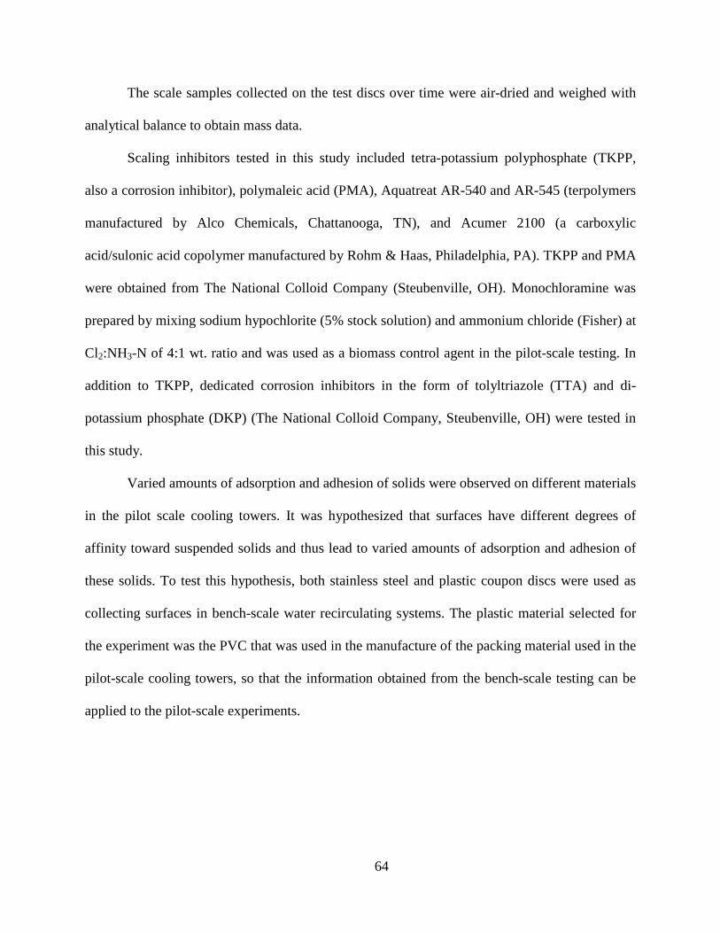
Figure 4.3 Predicted solid precipitation from the St. Vincent College Abandoned Mine Drainage calculated by
MINEQL+.
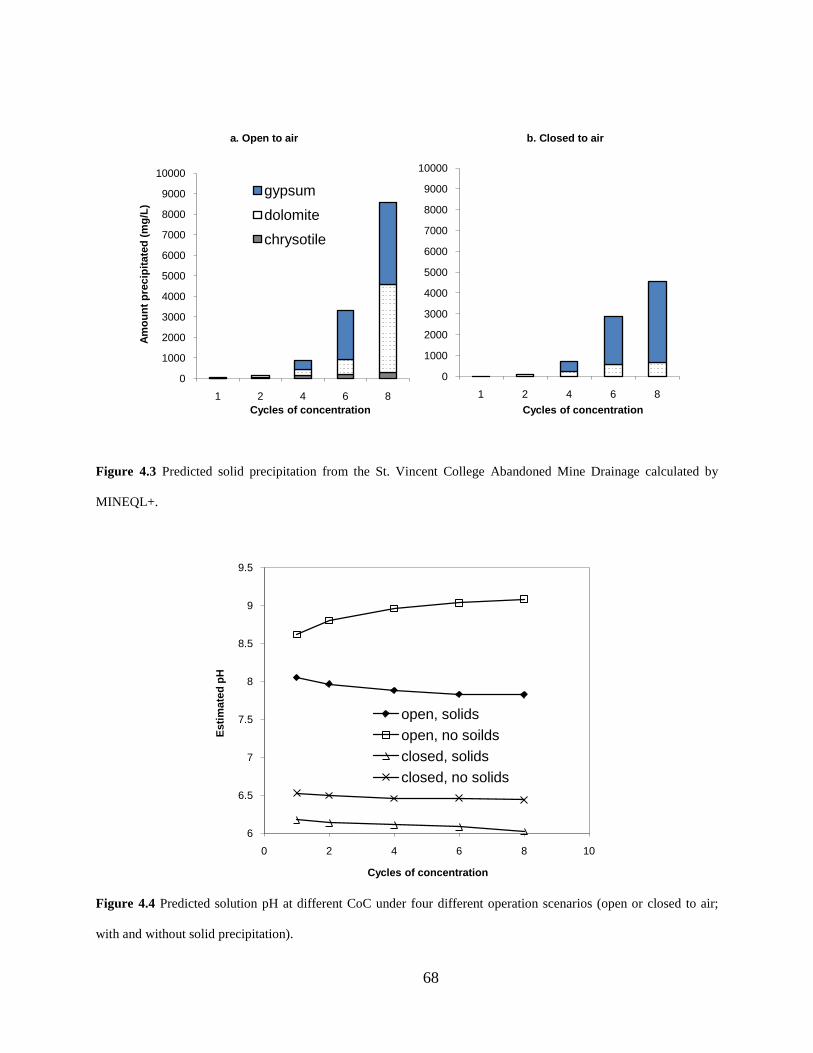
Figure 4.4 Predicted solution pH at different CoC under four different operation scenarios (open or closed to air;
with and without solid precipitation).
0
1000
2000
3000
4000
5000
6000
7000
8000
9000
10000
1 2 4 6 8
Amou
nt p
reci
pita
ted
(mg/
L)
Cycles of concentration
gypsumdolomitechrysotile
0
1000
2000
3000
4000
5000
6000
7000
8000
9000
10000
1 2 4 6 8Cycles of concentration
6
6.5
7
7.5
8
8.5
9
9.5
0 2 4 6 8 10
Estim
ated
pH
Cycles of concentration
open, solidsopen, no soildsclosed, solidsclosed, no solids
69
MINEQL+ modeling results suggest that gypsum and dolomite are the major solid
precipitates to form from the St. Vincent College abandoned mine drainage under recirculating
cooling tower conditions. More solids were predicted to precipitate under open-to-air condition
because of the abundant supply of carbonation. As shown in Figure 4.3, a significant amount of
otherwise dissolved solids could precipitate and contribute to solids accumulation when the
towers operate at high cycles of concentration. The amount of solids precipitation at equilibrium
was predicted to be 7-10 times more at CoC 8 than at CoC 4.
When the calculations allowed water to be open to the atmosphere and to equilibrate with
CO2(g), the pH values ranged between 8 and 9. When the calculations were performed in the
absence of exposure to the atmosphere, the water was predicted to become acidic. Under the
open condition, the calculated pH tended to increase with increasing CoC, when no solids were
allowed to form. Such behavior was due to the accumulation of alkalinity with CoC. On the other
hand, the pH tended to decrease with increasing CoC when solids formation was allowed to take
place because the alkalinity was consumed through dolomite formation.
4.3.2 Bench-scale recirculating system experiments
Two bench-scale water recirculating systems were used to determine the scaling behavior of the
actual SVAMD water at CoC 4 when inhibitors (i.e., PMA or AR-545) were added. The
SVAMD water in both systems was treated with 15 ppm anti-scalant: System A with AR-545
and System B with PMA. SVAMD samples were added to the two water recirculating system
and the water volume was reduced by 75% to CoC 4 with a heat source in about 5 days.
Concentration cycles, as determined by solution conductivity (which was the approach
for field testing), took a longer time to reach CoC 4 than that based on water volume reduction
70
(Figure 4.5). This suggests that the dissolved solids that precipitated during the concentrating
process do not contribute to the conductivity measurements. The 1:1 trend line defines an ideal
behavior by which all dissolved solids remain in solution during evaporative concentration. A
deviation from the 1:1 line indicates that part of the dissolved solids has precipitated out of the
solution during concentration. In the presence of anti-scalants, the degree of deviation from the
ideal line indicates the effectiveness of the added antiscalants to hold the solids in solution.
Using this criterion, it was determined that PMA was more effective.
Figure 4.5 Correlation of concentration cycles determined by water volume reduction and conductivity
measurements.
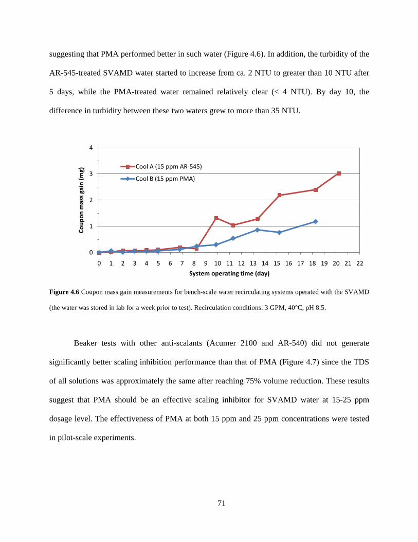
Coupon discs immersed in the SVAMD water treated with 15 ppm of AR-545 collected
more solids after 8 days than those immersed in the SVAMD water treated with 15 ppm of PMA,
1
2
3
4
5
6
1 2 3 4 5 6
CoC
base
d on
con
duct
ivit
y in
crea
se
CoC based on water volume reduction
Cool A (15 ppm AR-545)
Cool B (15 ppm PMA)
1:1 line
71
suggesting that PMA performed better in such water (Figure 4.6). In addition, the turbidity of the
AR-545-treated SVAMD water started to increase from ca. 2 NTU to greater than 10 NTU after
5 days, while the PMA-treated water remained relatively clear (< 4 NTU). By day 10, the
difference in turbidity between these two waters grew to more than 35 NTU.
Figure 4.6 Coupon mass gain measurements for bench-scale water recirculating systems operated with the SVAMD
(the water was stored in lab for a week prior to test). Recirculation conditions: 3 GPM, 40°C, pH 8.5.
Beaker tests with other anti-scalants (Acumer 2100 and AR-540) did not generate
significantly better scaling inhibition performance than that of PMA (Figure 4.7) since the TDS
of all solutions was approximately the same after reaching 75% volume reduction. These results
suggest that PMA should be an effective scaling inhibitor for SVAMD water at 15-25 ppm
dosage level. The effectiveness of PMA at both 15 ppm and 25 ppm concentrations were tested
Figure 4.7 Effectiveness of different antiscalants in beaker tests at 40-45°C.
Initial water volume was 1.00 L, final volume for TDS measurements was 0.25 L. Water was heated in a water bath
and bubbled with air to facilitate evaporation. It took 1-1.5 days for the water to reach CoC 4 (i.e., water volume
reduction from 1.00 L to 0.25 L).
Figure 4.8 shows that the PVC discs collected more solids from water, especially in the
absence of PMA, than the stainless steel coupons. On average, 3-4 times more solids were
collected on the PVC than on the stainless steel.
4400
4600
4800
5000
5200
5400
5600
5800
6000
Blank AR-545 PMA Acumer 2100 AR-540
TDS
(mg/
L) o
f the
con
cent
rate
d w
ater
afte
r 4:
1 vo
lum
e re
duct
ion
Anti-scalant dosed at 15 ppm
73
Figure 4.8 Coupon mass gain measurement for bench-scale water recirculating systems fed with the SVAMD water.
The system was operated at 3 GPM, 40°C, and CoC 4. Upper panel: measured with stainless steel coupon discs.
Lower panel: measured with PVC coupon discs.
The bench-scale experiments led to two basic conclusions: a) PMA performed
satisfactorily well for scaling inhibition under the operating conditions employed; and b)
Conductivity-based control of concentration cycles could deviate significantly from the
concentration cycles determined based on water volume reduction.
74
Table 4.2 Cooling tower water quality in the field testing using the passively-treated AMD from St. Vincent College
mine drainage site
The recirculating tower water analyzed was operated at CoC 4 (the run from October 18, 2008 to November 9,
2008). Unit: mg/L
Analyte Result (unfiltered)
Tower A Tower B Tower C Al ND ND ND Ca 825 674 796 Cu 0.0629 0.0303 B 0.0344 B Fe ND ND ND K 29.3 23.4 26.3 Mg 254 251 235 Mn 0.578 0.109 0.595 Na 446 450 418 SiO2 59.1 57.9 54.9 Zn 0.0567 0.101 0.0531
NH3-N 0.57 J 0.74 J 0.64 Bicarbonate
Alkalinity 276 J 92.3 J 257 J BOD ND ND ND Cl 216 239 223 NO3-N 1.1 1.1 1.1 SO4 2930 J 2910 J 2850 J Total P 0.64 0.032 B 0.65 Total Alkalinity 407 92.3 J 400 J TOC 13.8 6 17
Notes: J: Method blank contamination. The associated method blank contains the target analyte at a
reportable level. B: Estimated result. Result is less than reporting limit. ND: Not detected.
75
4.3.3 Pilot-scale study
Bulk water chemistry in cooling towers. The water quality data for the three cooling towers are
summarized in Table 4.2, and discussed in detail below.
pH – The pH values in towers treated for scaling inhibition by PMA (along with other
chemical additives for simultaneous corrosion and biofouling control) were different from those
in the control tower. The control tower (Tower B) that had no PMA addition had an average pH
of 8.2, whereas the two towers that received chemical treatments for scaling, corrosion, and
biofouling control had an average pH value of 8.7 for Tower A and 8.8 for Tower C. As a
reference, the raw SVAMD had an average pH of 7.8. The comparatively higher pH levels in the
treated towers were related to the higher levels of solution alkalinity that was retained by PMA.
Chloride – Chloride concentrations in the recirculating water were generally 6-8 times
greater than those in the makeup water (i.e., 400 mg/L in recirculating vs. 60 mg/L in makeup).
As such, the values of CoC based on the chloride concentration were also greater than the
volume-based values of CoC 4-5. The extra amount of chloride input was from the addition of
chlorine-based biocide (i.e., in the form of monochloramine).
Sulfate – Sulfate concentrations in the towers were generally 4-5 times higher than those
in the makeup water. This ratio was close to the volume-based CoC since there was no additional
sink or source of sulfate (gypsum was not found in solid deposits).
Phosphate – Orthophosphate was added as a corrosion inhibitor. The target phosphate
concentration was 5 ppm as PO43- but it was not strictly maintained due to its low solubility in
the presence of high concentration of calcium. Consequently, phosphate concentrations in the
bulk water remained below 1 ppm. Corrosion studies showed that the added phosphate (in the
76
form of pyrophosphate) was ineffective to prevent corrosion. Rather, the addition of phosphate
produced more phosphate-containing scales.
Alkalinity – Alkalinities in Towers A and C were around 4 times higher than those in the
makeup water, close to the volume-based CoC. However, in Tower B, the alkalinity was close to
makeup water. The significant difference in alkalinities between the test towers and the control
tower is attributed to the addition of PMA. Without PMA addition in Tower B, alkalinity was
consumed by the formation of calcium carbonate precipitates. In Towers A and C, PMA
successfully inhibited the formation of calcium carbonates and as a result, most of the alkalinity
remained in the aqueous phase.
Mass deposition over time. During the pilot-scale testing with the SVAMD water, a
preliminary run was conducted for a period of 12 days as a test run to obtain critical data for
cooling tower performance. Figure 4.9 (upper panel) depicts the time course of scale mass
deposited on stainless steel coupon discs in the three towers during the preliminary run. The
scale accumulation on the coupon discs was excessive- the entire coupon surface was covered by
a thick layer of deposits (ca. 2 mm thick). The excessive solids deposition was caused by the
towers operating at much higher cycles of concentration than originally planned. The towers
were operated at higher CoC because the conductivity probes in each tower that were used to
monitor the conductivity of the recirculating water and to trigger blowdown at preset values
failed to function properly. The experiment was designed to operate with raw SVAMD with an
average conductivity of 1.91 mS/cm, which means that the recirculating water in each tower
should have conductivity values between 7.5-9.5 mS/cm to maintain a target CoC of 4-5.
However, tower blowdown was not successfully triggered at these predetermined conductivity
77
levels and the towers were actually operating at CoC 8-10 based on water volume reduction. The
excessive mass deposition observed was consistent with modeling predictions (Figure 4.3).
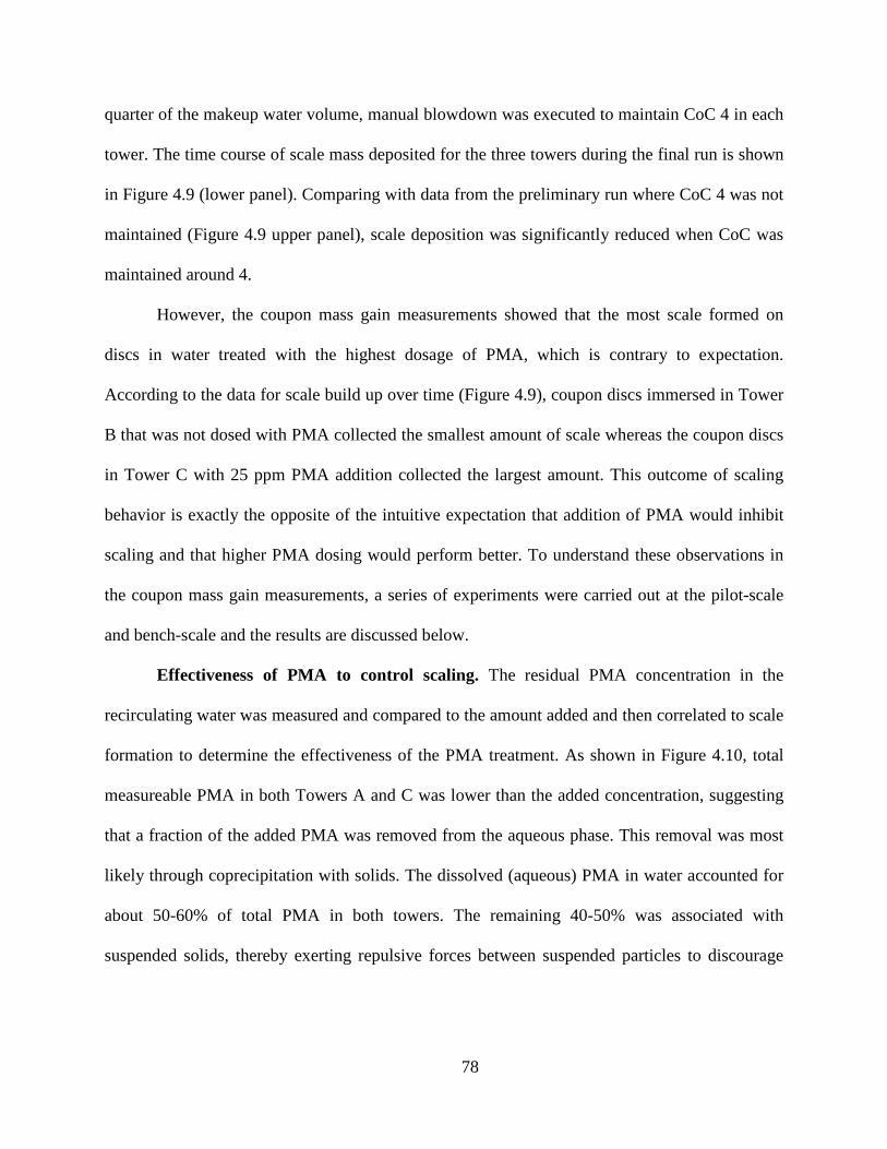
Figure 4.9 Mass gain measurements in pilot-scale cooling towers operated with SVAMD water at FTMSA site.
Upper: preliminary test run (CoC 8-10); Lower: final run (CoC 4-5). Deposits were collected on stainless steel
coupon discs immersed in pipe flow. Effective collection area 5.61 cm2, flow velocity 1.9 ft/sec (3 GPM in 3/4" ID
pipe), water temperature 104 ± 2°F in the pipe section, open recirculating cooling system.
Upon completion of the preliminary run, the conductivity probes were either calibrated or
replaced to ensure proper function prior to the final run. To guarantee proper blowdown when
the towers reached CoC 4, daily check up on the blowdown volume was performed throughout
the run. When the volume of blowdown based on the conductivity measurements was less than a
78
quarter of the makeup water volume, manual blowdown was executed to maintain CoC 4 in each
tower. The time course of scale mass deposited for the three towers during the final run is shown
in Figure 4.9 (lower panel). Comparing with data from the preliminary run where CoC 4 was not
maintained (Figure 4.9 upper panel), scale deposition was significantly reduced when CoC was
maintained around 4.
However, the coupon mass gain measurements showed that the most scale formed on
discs in water treated with the highest dosage of PMA, which is contrary to expectation.
According to the data for scale build up over time (Figure 4.9), coupon discs immersed in Tower
B that was not dosed with PMA collected the smallest amount of scale whereas the coupon discs
in Tower C with 25 ppm PMA addition collected the largest amount. This outcome of scaling
behavior is exactly the opposite of the intuitive expectation that addition of PMA would inhibit
scaling and that higher PMA dosing would perform better. To understand these observations in
the coupon mass gain measurements, a series of experiments were carried out at the pilot-scale
and bench-scale and the results are discussed below.
Effectiveness of PMA to control scaling. The residual PMA concentration in the
recirculating water was measured and compared to the amount added and then correlated to scale
formation to determine the effectiveness of the PMA treatment. As shown in Figure 4.10, total
measureable PMA in both Towers A and C was lower than the added concentration, suggesting
that a fraction of the added PMA was removed from the aqueous phase. This removal was most
likely through coprecipitation with solids. The dissolved (aqueous) PMA in water accounted for
about 50-60% of total PMA in both towers. The remaining 40-50% was associated with
suspended solids, thereby exerting repulsive forces between suspended particles to discourage
79
solids settling (PMA molecules are generally negatively charged due to dissociation of
carboxylic groups).
Figure 4.10 Total PMA (left panel) and dissolved (aqueous) PMA (right panel) concentrations in the recirculating
water of the cooling towers as measured after daily addition of PMA (with 0.5 hr delay).
PMA dose was based on water blowdown volume. The aqueous PMA concentration was obtained by filtering the
water sample through a 0.22-μm filter. Background readings were corrected using water sampled from Tower B
where no PMA was added.
The effect of PMA as an antiscalant was contrary to the original hypothesis that PMA
would reduce scale formation; higher concentrations of PMA in the recirculating water resulted
in more scale deposition on the steel coupons. Additional experiments determined that a
significant amount of solids were precipitated on the packing in Tower B, which did not receive
any antiscalant (the PVC surface exhibited significant affinity for the SVAMD solids) and that
the turbidity of the recirculating water in Tower B was close to that of the makeup water (Figure
4.11). The large error bars (one standard deviation) of the turbidity measurements (Figure 4.11)
80
with waters in Towers A and C suggest that the differences in turbidity of the two waters are
statistically insignificant: both waters contained appreciable amount of suspended solids. Such
findings suggest that the solids formed in Tower B were easily separated from the liquid phase
and removed from the system. This was evidenced by the mass balance on four main sections of
the recirculating cooling tower system (Table 4.3). At the bottom sumps of the towers,
significant amounts of solids were accumulated under slow flow condition. For Tower B without
PMA treatment, solids buildup became the most serious in the tower packing section where
evaporative concentration led to precipitation-induced deposition. In Towers A and C, the
influence of flow rate in the bottom sump and the evaporation on the tower packing were
mitigated by the presence of PMA, which impeded solids deposition. Higher levels of suspended
solids in Towers A and C resulted in higher water turbidities and a greater chance for the
suspended solids to deposit on the pipe and coil sections. It is noteworthy that the ranking order
of the solids deposition at the pipe and coil section of the three cooling towers calculated based
on the mass balance analysis (i.e., C > A > B) is in agreement with the scaling trends measured
by the coupon mass gain (Figure 4.9).
81
Figure 4.11 Turbidity of the makeup water and the recirculating water in the cooling towers during the CoC 4
operation.
The column represents mean values of seven measurements over the course of tower operation; error bars represent
1 standard deviation of the seven measurements for each tower.
82
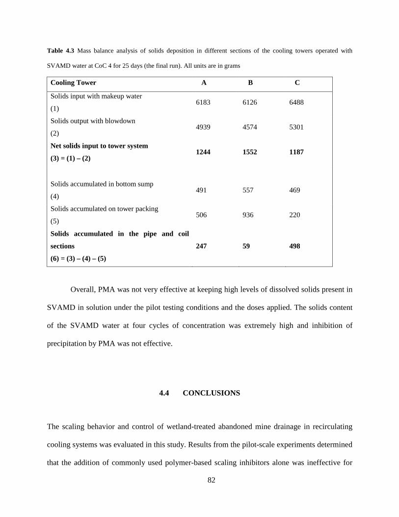
Table 4.3 Mass balance analysis of solids deposition in different sections of the cooling towers operated with
SVAMD water at CoC 4 for 25 days (the final run). All units are in grams
Cooling Tower A B C
Solids input with makeup water (1)
6183 6126 6488
Solids output with blowdown (2)
4939 4574 5301
Net solids input to tower system (3) = (1) – (2)
1244 1552 1187
Solids accumulated in bottom sump (4)
491 557 469
Solids accumulated on tower packing (5)
506 936 220
Solids accumulated in the pipe and coil
sections (6) = (3) – (4) – (5)
247 59 498
Overall, PMA was not very effective at keeping high levels of dissolved solids present in
SVAMD in solution under the pilot testing conditions and the doses applied. The solids content
of the SVAMD water at four cycles of concentration was extremely high and inhibition of
precipitation by PMA was not effective.
4.4 CONCLUSIONS
The scaling behavior and control of wetland-treated abandoned mine drainage in recirculating
cooling systems was evaluated in this study. Results from the pilot-scale experiments determined
that the addition of commonly used polymer-based scaling inhibitors alone was ineffective for
83
scaling control. The high concentration of total dissolved solids requires more comprehensive
pretreatment and scaling controls. Nevertheless, the added PMA, at concentrations of 15 to 25
ppm, lent some stability to suspended mineral solids (high water turbidities) and there was less
deposition in the pipe flow sections of the cooling towers.
Deposits from the SVAMD concentrated to CoC 4 in recirculating cooling systems
exhibited varied affinities to different surfaces. More deposits were collected on the PVC
surfaces that were used as the tower packing material. Hydrodynamics also played a role in
deposition. Low flow velocities encountered in the plastic packing and bottom sump sections of
cooling tower resulted in greater sedimentation. Indeed, significant amount of deposits were
observed at the bottom of the tower sump, especially in the tower receiving no PMA treatment.
The finding suggests that scaling took place in a nonuniform manner throughout the cooling
tower system. Therefore, it is suggested that scaling measurements should be performed at tower
sections where deposition is of concern. Also, similar materials of test coupon should be used for
scale deposition to provide substrate surfaces representative of the building materials of cooling
tower.
84
5.0 SCALING CONTROL IN ASH TRANSPORT/SETTLING POND WATER
INTERNALLY USED IN COAL-FIRED POWER PLANT COOLING SYSTEMS
Water sluicing systems are commonly used at coal-fired electric power plants to remove
combustion residues, i.e., fly ash and bottom ash, from the plant. Water is used to transport the
ash to sedimentation ponds where the ash is hydraulically settled and the supernatant—ash pond
effluent (APW)—is discharged. APW is a promising alternative to freshwater as a cooling water
makeup for coal-fired power plants, as it is internally available at many plants. The amounts of
APW available at a coal-fired power plant can generally satisfy the cooling water makeup needs
in a recirculating cooling system. The reuse of APW, which contains a variety of soluble
chemicals originated from coal-ash leaching, can avoid their direct discharge to natural waters,
which can be potentially problematic since the APW contains a variety of soluble chemical
contaminants originated from the leaching of the sluiced coal ash. But concentrated APW in
recirculating cooling systems may cause scaling problems. In this study, the feasibility of
controlling scaling when using clarified APW, the pond effluent after the ash solids are settled,
in cooling water systems was investigated through laboratory experiments. Bench-scale
recirculating experiments were conducted to test chemical control schemes for scaling in systems
APW. The testing was conducted at temperature, flow velocity conditions as well as water
constituent concentrations similar to those in a recirculating cooling system. The effectiveness of
chemical treatment strategies in inhibiting scaling was studied through exposure and monitoring
85
of specially designed disc specimens in extended duration tests. The mineral scaling resulting
from the use of the APW was much less severe than from the previously tested two other
impaired waters (i.e., secondary-treated municipal wastewater and passively-treated abandoned
mine drainage). The addition of PMA (10 ppm) effectively inhibited scale formation, while
without PMA treatment the scale formed consisted of primarily calcium solids. In addition, this
study demonstrated that the corrosion products from the metallic components of cooling towers
could potentially lead to elevated amounts of scales due to the re-deposition of the corrosion
product solids, especially under the conditions where large metallic surface is in contract with
the APW cooling water.
5.1 INTRODUCTION
Ash transport water is typically regarded as expendable waste because after sedimentation, the
sluicing water effluent from the sedimentation ponds is usually discharged into receiving waters.
A variety of soluble chemical species are present in ash transport water as a result of leaching
from the fly bottom ashes and in some cases from addition of plant liquid wastes to the sluice
water. Fly ash and bottom ash generally contain little organic matter. The chemical constituents
of most concern in ash transport water with respect to discharge are inorganic, in particular
metals [1, 2]. These are derived from leaching of ash particles, which consist primarily of oxides
of silicon, aluminum, and iron, but also contain a number of other metals at lower levels.
Impaired waters are of increasing interest as alternative sources of makeup water for
thermoelectric power plant recirculating cooling water systems. Ash transport water has the
potential for use in cooling systems at coal-based power plants. The large amounts of water
86
involved in these processes represent a substantial opportunity for internal water reuse in cooling
systems at electric power plants. In most case the ash transport slurries are directed into
sedimentation ponds in which settling of the ash particles takes place. There is potential to reuse
a portion or all of the ash pond effluent, as has been investigated periodically in the past [3].
The amount of ash transport water available at a coal-fired power plant generally can
satisfy the cooling water need for the recirculating system in the power plant. The mean value of
bottom ash pond overflow is 3,881 GPD/MW [4], which can contribute 27% of the mean value
of makeup water needs, in recirculating cooling system, which averages 14,400 GPD/MW [5].
The objective of this study was to investigate the scaling potential of APW under the
conditions commonly encountered in recirculating cooling water systems and study the
effectiveness of some commonly used scaling inhibitors. Specifically, scale formation of the
APW was calculated at different cycles of concentration (CoC) under relevant cooling tower
operation conditions using the chemical equilibrium model MINEQL+. The actual APW taken
from Reliant Energy Power Plant ash settling pond effluent was tested in a bench-scale water
recirculating system to examine its scaling behavior under CoC 1 vs. CoC 4. Synthetic APW was
then used to better represent CoC 4 condition. The effectiveness of different antiscaling
chemicals were tested using synthetic APW.
87
5.2 MATERIALS AND METHODS
5.2.1 Ash Pond Water Characterization and Preparation for Laboratory Testing
APW from the Reliant Energy coal-based thermoelectric power plant, located at Cheswick, PA,
was used for testing in laboratory experiments, as well as for equilibrium chemical modeling.
Water samples were collected on October 2, 2007, and analyzed for a range of water quality
constituents [6]. The water samples were collected with a 1-L polyethylene sampler and then
transferred to appropriate polyethylene or glass sample containers provided by the commercial
laboratory, TestAmerica (Pittsburgh, PA). Appropriate preservatives were added to the sample
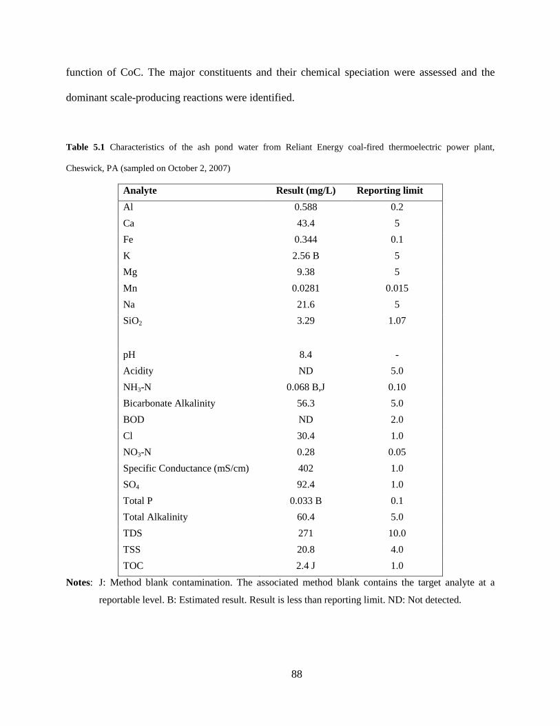
bottles prior to sampling. Analyses performed are summarized in Table 5.1.
Parallel to the sampling for chemical analysis, a larger amount of the APW was collected
for laboratory experiments. The water was concentrated in the laboratory by heat evaporation at
35-40°C to reach 4 cycles of concentration (CoC 4) as determined by 75% water volume
reduction. This concentration level is representative of the CoC used in recirculating cooling
tower systems operated with impaired waters.
5.2.2 Equilibrium Modeling of APW Scaling Potentials
The chemistry of the APW cooling water at different CoC was modeled using MINEQL+ [7, 8]
to gain insight into the effects of CoC on scaling. The primary objective for this effort was to
estimate the amount and composition of mineral solids that would precipitate and the water
chemical composition that would occur under typical cooling tower operation conditions as a
88
function of CoC. The major constituents and their chemical speciation were assessed and the
dominant scale-producing reactions were identified.
Table 5.1 Characteristics of the ash pond water from Reliant Energy coal-fired thermoelectric power plant,
Cheswick, PA (sampled on October 2, 2007)
Analyte Result (mg/L) Reporting limit Al 0.588 0.2 Ca 43.4 5 Fe 0.344 0.1 K 2.56 B 5 Mg 9.38 5 Mn 0.0281 0.015 Na 21.6 5 SiO2 3.29 1.07 pH 8.4 - Acidity ND 5.0 NH3-N 0.068 B,J 0.10 Bicarbonate Alkalinity 56.3 5.0 BOD ND 2.0 Cl 30.4 1.0 NO3-N 0.28 0.05 Specific Conductance (mS/cm) 402 1.0 SO4 92.4 1.0 Total P 0.033 B 0.1 Total Alkalinity 60.4 5.0 TDS 271 10.0 TSS 20.8 4.0 TOC 2.4 J 1.0
Notes: J: Method blank contamination. The associated method blank contains the target analyte at a
reportable level. B: Estimated result. Result is less than reporting limit. ND: Not detected.
89
The following four operational conditions were simulated for the APW water:
1) The aqueous system was open to the atmosphere (PCO2 = 10-3.5 atm) to allow the
alkalinity to be in equilibrium with CO2(g) and solids were allowed to precipitate.
2) The aqueous system was open to the atmosphere (PCO2 = 10-3.5 atm) to allow the
alkalinity to be in equilibrium with CO2(g) and solids were not allowed to precipitate (i.e., water
can be super-saturated).
3) The aqueous system was closed to the atmosphere with total alkalinity fixed and solids
were allowed to precipitate.
4) The aqueous system was closed to the atmosphere with total alkalinity fixed and solids
were not allowed to precipitate.
The four conditions represent the extreme effects of atmospheric CO2 and solution
supersaturation. It is reasonable to expect that the actual conditions for field testing would fall
within these boundary conditions.
5.2.3 Bench-scale Tests with REAPW
The objective of the bench-scale studies with APW was to test the effectiveness of different
scaling inhibition chemicals, added either individually or in proper combinations. The
experimental system was depicted in Figure 5.1. Four antiscalants were tested whose selection
was based on a literature review and consultation with experts in the cooling industry. The
antiscalants were polyacrylic acid (PAA), polymaleic acid (PMA), 2-phosphonobutane-1,2,5-
tricarboxylic acid (PBTC), and tetrapotassium pyrophosphate K4P2O7 (TKPP). PAA and PMA
are short-chain organic polymers, while PBTC and TKPP are phosphorous-based (i.e.,
phosphates/phosphonates) common antiscalants. At the start of each experiment, an antiscalant
90
was added to the recirculating water. The combination of PMA and PBTC at a dosing ratio of
2:1, as recommended by cooling experts for better performance, was also tested. In addition, the
effect of cycles of concentration (CoC) was examined with an actual ash pond effluent from
Reliant Energy power plant.
Figure 5.1 Bench-scale water recirculating system with inserted stainless steel circular disc specimens for scale
collection and subsequent mass gain measurement.
Inset shows a pipe T-section where stainless steel circular disc specimens were inserted. Both actual and synthetic
APW was tested.
91
5.3 RESULTS AND DISCUSSION
5.3.1 Precipitation Modeling with Equilibrium Calculations
The chemical equilibrium model MINEQL+ (version 4.5) was used in detailed evaluation of the
cooling water chemistries. Scaling potentials at different cycles of concentration, as measured by
the two most commonly referenced practical saturation indexes and direct predictors of
precipitation formation, were analyzed. The pH values with respect to cycles of concentration
were also calculated.
Detailed modeling results consist of the following:
The Langelier Saturation Index (LSI) and Ryznar Stability Index (RSI) under open/closed
conditions as a function of CoC (Figure 5.2);
Figure 5.2 Modeling results of LSI (left) and RSI (right) for both open and closed to air cases, Reliant Energy ash
pond water.
-1
-0.5
0
0.5
1
1.5
2
2.5
3
0 2 4 6 8 10
Lang
elie
r sat
urat
ion
inde
x (L
SI)
Cycles of concentration
Open
Closed
0
1
2
3
4
5
6
7
8
0 2 4 6 8 10
Ryz
nar s
tabi
lity
inde
x (R
SI)
Cycles of concentration
Open
Closed
92
Amount and form of solid precipitates under open/closed conditions as a function of
CoC (Figure 5.3);
Changes of aqueous pH with increasing CoC (Figure 5.4).
a. Open to air b. Closed to air
Figure 5.3 Predicted solid precipitation from the Reliant Energy ash pond water, calculated by MINEQL+.
0
50
100
150
200
250
300
350
400
450
500
1 2 4 6 8
solid
pre
cipi
tatio
n (m
g/L)
Cycles of concentration
0
50
100
150
200
250
300
350
400
450
500
1 2 4 6 8Cycles of concentration
diasporedolomitecalcitechrysotile
93
Figure 5.4 Predicted solution pH at different CoC under four different operation scenarios (open or closed to air;
solid precipitation is allowed or not), Reliant Energy ash pond water.
The Langelier Saturation Index (LSI) increased with cycles of concentration, so did the
scaling potential. For the Ryznar Stability Index (RSI), it was calculated by a different formula
and usually exhibited an opposite trend compared to the LSI. The RSI values in Figure 5.2
decreased with the cycles of concentration (as did the corrosion potential). Under all conditions,
RSI values were below 8, indicating mild corrosion potentials.
Calcite and dolomite are the major solid precipitates predicted by MINEQL+ to form in
the Reliant Energy ash pond water under typical recirculating cooling tower conditions. From
Figure 5.3, greater amount of solids precipitated out of solution when operated at an open-to-air
condition, because under this condition CO2 was allowed to be dissolved from the air into
solution to provide carbonate species for the formation of calcite and dolomite. Nevertheless,
6
6.5
7
7.5
8
8.5
9
9.5
0 2 4 6 8 10
Estim
ated
pH
Cycles of concentration
open, solids open, no soilds
closed, solids closed, no solids
94
solids formation from the APW water was very minimal compared to other impaired waters
studied in this project.
When the water was open to the atmosphere to allow equilibrium with CO2(g), the pH
values were between 8 and 9. When the water was closed to the atmosphere, the water became
acidic. Under open condition, the pH tended to increase with increasing CoC when no solids
were allowed to form. This was because of the accumulation of alkalinity with CoC. On the other
hand, the pH tended to decrease with increasing CoC when solids formation took place because
the alkalinity was consumed by the formation of calcite and dolomite.
5.3.2 Bench-scale Recirculating System Experiments
Tests with actual APW. Interesting scaling behaviors were observed when comparing the
amounts of deposit over time in the actual ash pond water at CoC 1 vs. CoC 4 (Figure 5.5). After
the water was recirculated in a bench-scale water recirculating system for 120 h (5 d), more
deposits were collected from the CoC 1 water. This observation was contrary to expectations
because the water at CoC 1 (i.e., un-concentrated raw water) should contain only one quarter of
the amounts of mineral solutes than the CoC-4 water, and thus would be much less scale
forming. Results depicted in Figure 5.6, which compares the predicted and measured TDS in
APW that was being concentrated by evaporation, offered an explanation for this discrepancy.
During the concentration process of water evaporation to reach CoC 4, a portion of the mineral
solids was precipitated out of solution. As a result, the TDS contained in the CoC-4 water (the
CoC was determined by a 75% water volume reduction) was less than four times of the TDS
contained in the raw (CoC-1) water. On the same figure, the results from modeling prediction by
MINEQL+ provided similar trend.
95
Figure 5.5 Scaling behavior of the Reliant Energy ash pond effluent in bench-scale water recirculating tests: effect
of cycles of concentration (CoC).
Experimental conditions: 40°C and 3 GPM. For CoC-4 tests, the water was pre-concentrated by evaporation in a
heating bath (40°C) to lose 75% volume before adding to the recirculating system.
Figure 5.6 Changes in solution TDS as a function of CoC for Reliant Energy ash pond water.
Theoretically, TDS should increase linearly with increasing CoC (dashed line). However, as CoC increases, both
MINEQL+ predictions (open circles) and experimental observations (filled circles) deviated from the theoretical
curve. The TDS measurements were performed with actual water concentrated by water evaporation.
0
1
2
3
0 24 48 72 96 120144168192216D
epos
its
(mg)
Time (h)
CoC 1 (a)
CoC 4 (b)
0
100
200
300
400
500
600
700
800
900
1 2 3 4 5
TDS
(mg/
L)
CoC
TheoreticModel predictedMeasured
Theoretical Predicted Measured
96
Loss of mineral solids during evaporation did not, however, fully explain the reversal in
the scaling of the actual APW at CoC 1 vs. CoC 4. To further explore the causes of this
interesting behavior, the chemical composition of the scale collected from both waters was
analyzed by energy dispersive X-tray spectrometry (EDS). The analysis revealed a significant
amount of iron in the scale produced from the CoC-1 water (data not shown). Given the fact that
the actual APW sampled from Reliant Energy contained very little iron (< 1 mg/L), it is inferred
that the iron-laden deposit came from the corrosion of mild steel coupons that were inserted for
simultaneous corrosion studies in the same recirculating system. This was corroborated by the
fact that the average corrosion rate of the mild steel was 105 MPY, which was more than 10
times greater than the corrosion rate observed in the concentrated APW (CoC 4). Three other
corrosion-study coupons made of aluminum, copper, and copper-nickel were also present in the
recirculating water but their corrosion rates were negligible compared to the mild steel. To
remove the complications of mild steel corrosion on scaling determination, other experiments
were performed with corrosion coupons removed from the system, unless stated otherwise
(corrosion studies were continued using a separate recirculating system).
The significance of corrosion complications to scaling depends on the relative amounts of
iron oxidized and released from the mild steel coupons to water. In the bench-scale recirculating
system, the amounts of iron corroded and added to the recirculating water were significant in the
relatively small volume of water used (i.e., 2-3 L of total water for each experiment). On the
other hand, corrosion may not affect scaling as much in the field testing even when both
corrosion and scaling coupons are used simultaneously, because the water volume contained in a
cooling tower is much greater (e.g., 75 L in our pilot-scale cooling tower). Nevertheless, these
findings are indicative in that scaling determination in industrial cooling systems should be
97
carefully executed to take into account the potential contributions of corrosion products to scale
formation.
Tests with synthetic APW. Based on the observation in the actual APW at CoC 1 vs.
CoC 4 as discussed in the previous section, it was decided to use a synthetic APW water that
truly simulated the chemical composition of the CoC-4 APW, in the study of APW scaling and
its control by different antiscalants. The chemical composition of the synthetic APW used is
listed in Table 5.2. The effectiveness of scaling control by PAA, PMA, and PBTC was examined
first with individual tests of each agent (Figure 5.7). PAA was less effective than PMA, which
was equally effective as PBTC. To further test the synergistic effect of polymer and phosphonate
at a 2:1 dosing ratio, which is a widely adopted mix ratio in industrial practices for scaling
control in cooling systems [9], PMA and PBTC dosed at 10 ppm and 5 ppm respectively were
added to the synthetic ash pond water (CoC 4). It was observed that the addition of 5 ppm of
PBTC to 10 ppm of PMA further improved the antiscaling effectiveness but not to a significant
degree (the difference in the scale mass was less than 10%).
Figure 5.7 Scaling behavior of synthetic ash pond effluent in bench-scale tests: effectiveness of different
antiscalants at CoC 4.
0
1
2
3
0 24 48 72 96 120 144
Dep
osit
s (m
g)
Water recirculating time (hr)
Control (CoC 4)
PAA 10ppm
PMA 10ppm
PBTC 10ppm
PMA-PBTC 10/5ppm
98
Table 5.2 Chemical composition of synthetic ash pond water effluent (representing 4 cycles of concentration)
Cation Concentration
mM mg/L Anion
Concentration
mM mg/L
Ca2+ 4.41 177 SO42- 4.08 392
Mg2+ 1.63 39.6 HCO3- 5.12 312
Na+ 9.45 217 Cl- 8.81 312
Fe3+ 0.28 15.6
Note: The Fe concentration used in the synthetic water represents an average iron concentration level among
Figure 7.4 shows the different patterns of mineral precipitation as measured by the changes in
solution conductivity with different doses of PMA addition. Without PMA, precipitation started
at about 1.5 hr, and was essentially completed within a few minutes. With PMA addition, the
onset of precipitation was delayed. Even with just 0.1 ppm of PMA, the precipitation started after
4.8 hr, which is delayed by 3.3 hr compared to the case without PMA. With greater amounts of
PMA added to the solution (0.5 ppm, 1 ppm, and 5 ppm), the induction times were delayed even
further; with 5 ppm of PMA, precipitation started after 15.6 hr. Not only were the induction
times delayed with PMA, but the precipitation rates (the slopes of the conductivity change with
time) were also slower with greater PMA addition. When the PMA concentration was increased
to 10 ppm, no “fast precipitation” was identified over the entire experimental period (50 hr).
The effect of PMA on the delay of the onset of mineral precipitation can be explained by
the reduction of the mineral solution supersaturation level in the presence of this organic
polymer. PMA molecules dissolved in solution may effectively interfere with the diffusivity of
139
the mineral ions, thereby reducing the driving force and chances of clustering and nucleation.
Also, the interactions between PMA molecules and newly-formed mineral surfaces may reduce
the magnitude of coefficient 𝑛 in Equation (7) or (8), thus decreases the precipitation reaction
rates.
7.4.2 Solid characteristics and chemical composition of the precipitate
For a more detailed evaluation of the retardation effect by PMA, the mineral precipitate from the
experiments with no PMA and 5 ppm of PMA (Figure 7.5) was collected and analyzed. In
addition, the mineral suspension without PMA addition at time zero was split into two equal
volumes and 5 ppm of PMA was added to one of the suspensions for further examination of the
PMA effect on pre-formed suspended particles. The SEM images of the mineral particles
collected from the three suspensions (at 48 hr) are shown in Figure 7.6. In the absence of PMA
(Figure 7.6-Left), the precipitate is comprised of multidispersed crystal pieces with highly
irregular shapes. With PMA added after the precipitate had formed, the crystal solids tend to
stick together to form clusters (Figure 7.6-Middle). In the case where PMA was added at the
beginning of experiment (before any precipitation took place), two distinct morphologies can be
identified, crystal and amorphous (Figure 7.6-Right).
140
Figure 7.5 Solution conductivity changes over time in the absence and presence of PMA (5 ppm, added at time 0).
Experimental condition: 750-mL solution in a Pyrex cell reactor, pH 7.5, 40°C, and 300 rpm. After precipitation
took place without PMA, the mineral suspension was split into two equal volumes (375 mL each) and 5 ppm of
PMA was added to one of the suspensions for the examination of the PMA effect on the deposition of mineral
particles.
PMA: 0 ppm PMA: 5 ppm added post
precipitation PMA: 5 ppm added at time zero
(prior to precipitation)
Figure 7.6 SEM images of the precipitated mineral particles collected under different PMA treatment.
Capital letters on images indicate the spots (areas) for EDS analysis.
2.55
2.6
2.65
2.7
2.75
2.8
2.85
0 6 12 18 24 30 36 42 48
Solu
tion
con
duct
ivit
y (m
S/cm
)
Time elapsed (hr)
PMA: 0 ppm
PMA: 5 ppm
Split suspension and add PMA (5 ppm) to one.
A
B C
D
141
To further reveal the effect of PMA on mineral precipitation, the elemental compositions
of the precipitate were determined by Energy Dispersive X-ray Spectroscopy (EDS, EDAX Inc.,
Mahwah, NJ). The relative signal intensities of the elements making up the precipitate are shown
in Figure 7.7. The precipitate appears to be a mixture of calcium phosphates and carbonates.
Surface adsorption of PMA that was added after bulk precipitation was evidenced by the
elevated peak intensities of C and O in Figure 7.7 upper panel. In the case where PMA was
added prior to bulk precipitation (Figure 7.7 lower panel), the elemental composition of the two
distinct morphologies (Figure 7.6-Right) was different. In the amorphous solids, more PMA was
incorporated than in the crystal structures. More importantly, with the amorphous formation,
appreciable amounts of Mg were also incorporated, which was not observed in other cases.
When curves (A) and (C) are compared in Figure 7.7, calcium carbonate formation is suppressed
by PMA, suggesting that calcium phosphate is more dominant in the presence of PMA.
0.00 1.00 2.00 3.00 4.00 5.00 6.00 7.00keVChart Title
(A) PMA 0 ppm
(B) PMA 5 ppm added after precipitation
Ca
P C
O
142
Figure 7.7 Elemental composition of the precipitated mineral particles collected after different PMA treatment.
Capital letters for each curve correspond to the scanning spots (areas) indicated in Figure 7.5.
7.4.3 Association/complexation of PMA with Mg2+, Ca2+, and K+
Figure 7.8 shows the concentrations of PMA that was free in solution, i.e., PMA not complexed
with the cationic species present in solution at different concentration levels. PMA exhibited
strong affinity toward Mg2+. At [Mg2+]0 = 10 mM (corresponding to solution I = 30 mM), more
than 50% of the PMA (2.6 ppm) was in complexed form, whereas with Ca2+ only 30% of the
PMA (1.6 ppm) was complexed. The strong affinity between Mg2+ and PMA was responsible for
Mg incorporation into the mineral precipitates (Figure 7.7), which was not detected in the
absence of PMA.
It is known that ligands such as CO32- and PO4
3- exhibit different affinities for Ca2+ and
Mg2+. Compared to Ca2+, Mg2+ has less affinity for inorganic ligands, as evidenced by the
0.00 1.00 2.00 3.00 4.00 5.00 6.00 7.00keVChart Title
(C) PMA 5 ppm crystals
(D) PMA 5 ppm amorphous solids
C
O
Mg
P
Ca
143
smaller values of Ksp (the first two columns of Table 7.6). With regard to organic ligands that
bear primarily carboxylate groups, Mg2+ cations tend to be more strongly associated with them
than Ca2+ cations do, forming more stable complexes (the last three columns of Table 7.6).
Furthermore, the carboxylate groups in humic acids (HAs) were confirmed to be responsible for
HA complexation with divalent cations [18]. The HA fractions rich in carboxyl carbon may
become smaller in size thus more diffusive when complexed with Mg2+ or Ca2+ as revealed by
NMR studies [18]. The improved diffusivity contributes to the easier incorporation of the
complexes into the mineral precipitates, effectively distorting the crystallization process.
On the other hand, the amount of calcium or magnesium complexed with PMA was
minimal compared to the total concentrations of the cations present in the bulk solution. The
repeating unit (base unit) of PMA is -CH(COOH)-, which has a “molecular weight” of 58 g/mol.
Accordingly, 1 ppm of PMA corresponds to 17.24 µM of the PMA base unit. In the test solution
containing 5 ppm of PMA, there were 86.21 µM of the PMA unit. Assuming two units complex
with one Ca2+ ion, only 1% of the Ca2+ present in solution will be complexed ([Ca2+]0 = 4.0 mM)
even under a maximum complexation capacity of the PMA. This calculation suggests that the
changes of calcium concentration due to PMA complexation were insignificant, and would not
contribute significantly to the inhibition of calcium precipitation.
144
Figure 7.8 Solution concentrations of free PMA that was not complexed with cationic species.
Initial PMA added: 5 ppm, solvent: DI water. Solution was equilibrated for 3 hr before PMA measurements. Error
bars indicate triplicate preparation of test solutions.
Table 7.6 Stability constants (complexation constants or solubility product constants) of ligands with calcium and
magnesium (usually measured at 25°C, 1 atm, and I = 0)
pK Ligand
CO32- PO4
3- CH3COO- Carbonate Phosphate Acetate Ca2+ 8.31 44.2-55.63 1.25 Mg2+ 5.02 25.24 1.35 1 8.48 for calcite and 8.36 for aragonite in Mark Benjamin2; 8.34 for calcite and 8.22 for aragonite in Snoeyink3.
2 Sneoyink3; 4.67 for MgCO3·3H2O in Morel and Hering4. 3 Hydroxylapatite in Mark Benjamin2 and Morel and Hering4. 4 Bobierrite Mg3(PO4)2·8H2O in Morel and Hering4. 5 1:1 complex in Morel and Hering4.
0.0
1.0
2.0
3.0
4.0
5.0
6.0
0 5 10 15 20 25 30 35
Free
PM
A (p
pm)
Solution Ionic Strength (mM)
KClCaCl2MgCl2
KCl CaCl2 MgCl2
145
7.4.4 Adsorption isotherm of PMA on SS surface
The data shown in Figure 7.9 reveal an interesting phenomenon where the suspended particles
formed in the presence of PMA (5 ppm) appear to be “sticky” to the reactor wall. When PMA
was not added to the solution, turbidity increased after just one hour due to the formation of
suspended solids in the bulk phase. Addition of 5 ppm of PMA from the start of the experiment
delayed solids formation by 16 hr. However, a steady decrease in turbidity was observed after 20
hr of contact to the point that the turbidity decreased to about 40% of the initial value observed
after 20 hr. The turbidity was only recovered when the suspension was vigorously stirred to re-
suspend the mineral particles that had accumulated on the reactor wall. This raises a question,
how did PMA increase mineral deposition on the reactor wall? Data from previous studies
demonstrate that PMA addition to supersaturated solution helped mitigate mineral scaling on
stainless steel disc specimens (Chapters 3-5). How does the stainless steel surface differ from the
reactor wall (Pyrex glass) with regard to PMA adsorption, if any? To answer these questions,
batch reactors of similar volume but made of different materials (i.e., stainless steel, Pyrex glass,
and PE plastic) were used to study the potential adsorption of PMA to the reactor walls.Figure
7.10 shows that within 12 hr of equilibration with 5 ppm of PMA initial concentration, PMA did
not adsorb onto any of the reactors significantly.
146
Figure 7.9 Suspension turbidity changes over time in the presence and absence of PMA (5 ppm, added at time 0).
Experimental condition: 750-mL solution in a Pyrex cell reactor, pH 7.5, 40 °C, and 300 rpm. * Solid circles show
measurements after the suspension was vigorously stirred to re-suspend the mineral precipitates that had
accumulated on the reactor wall.
0
20
40
60
80
100
120
0 6 12 18 24 30 36 42 48
Susp
ensi
on T
urbi
dity
(NTU
)
Time elapsted (hr)
PMA: 0 ppm
PMA: 5 ppm
PMA: 5 ppm (*)
147
Figure 7.10 Solution PMA concentration in batch reactors made of different materials.
PMA added: 5 ppm, solvent: DI water, pH = 7.5 (adjusted with NaOH). Solution was equilibrated for 12 hr before
taking measurements. Error bars indicate triplicate preparation of the test solutions. This Figure shows that PMA did
not adsorb onto the reactor wall significantly.
Moreover, the experimental data in Figure 7.11 show that no PMA adsorption to the
stainless steel surface was observed after 60 hr of equilibration in an aqueous solution containing
an initial PMA concentration of 12 ppm at pH 7.5.Figure 7.12 shows that no PMA adsorption to
the stainless steel surface was observed when the initial PMA concentration ranged from 0-20
ppm and the solution pH varied from 8.5 and 7.0.
Table 7.7 Amount (weight) of stainless steel wire used in each adsorption isotherm test with different amount of
Influence of PMA on EIS. Figure 9.4 shows the EIS at the stainless steel working
electrode (WE) surface before and after PMA addition (5 ppm) in a 10 mM of KCl solution.
Compared to the EIS collected without PMA, the addition of PMA (5 ppm) did not effect any
significant changes in EIS, even after 5 hr of contact with PMA. The capacitive impedance
became slightly greater in the presence of PMA only toward the end of the low AC frequencies
(the Nyquist plot of Figure 9.4). This slight increase of the capacitive impedance is expected in
that the PMA molecules present near the electrode surface in solution can serve as a diffusional
barrier that increases charge transfer resistance, which is a major contributor to the capacitive
impedance [2]. However, this influence did not impact the CPE evaluation in the Bode plot
(Figure 9.4), which produced CPE capacitance values in the range of 40.26 ± 0.12 µF/cm2 in the
three cases tested.
0
100
200
300
400
500
600
b(%
·cm
2 /m
g)
CaSO4 CaCO3 Ca-P 2-minerals MWW
)(mg/cm deposited mass mineral(%) ecapacitanc CPE of reduction
2=b
192
Figure 9.4 EIS at the stainless steel WE surface before and after PMA addition (5 ppm) in aqueous solution.
Solution IS I = 10 mM KCl at pH 7.5, 40 °C, and 300 rpm. EIS experimental conditions: AC potential perturbation
±10 mV biased at the system’s open circuit potential (OCP); frequency scan from 10-2 to 104 Hz; data sampling at 10
points/decade. a) Bode plot, and b) Nyquist plot.
-90
-80
-70
-60
-50
-40
-30
-20
-10
0
100
1000
10000
100000
1000000
0.01 0.1 1 10 100 1000 10000
Phas
e an
gle,
θ(°
)
Z (o
hm)
Frequency (Hz)
No PMA5 ppm PMA, 10 min5 ppm PMA, 5 hr
0
50000
100000
150000
200000
250000
0 20000 40000 60000 80000 100000
-Zim
ag(o
hm)
Zreal (ohm)
No PMA5 ppm PMA, 10 min5 ppm PMA, 5 hr
a)
b)
193
Influence of Chlorine Biocides on EIS. Figure 9.5 shows the EIS at the stainless steel
working electrode (WE) surface with different chlorine biocide additions in a 10 mM KCl
solution. Compared to the EIS collected without chlorine, the addition of either 1 ppm of free
chlorine or 2 ppm of monochloramine substantially altered the EIS response curves. The
alteration is apparent toward both ends of the AC scanning frequencies, i.e., < 0.1 Hz or > 1 kHz.
The EIS in the presence of free chlorine deviated from the reference EIS (i.e., EIS collected in
the absence of chlorine) to a greater extent than in the presence of monochloramine. This
deviation pattern suggests that the interference of the chlorines on EIS is related to the oxidation
power of the biocide, with free chlorine being more powerful than monochloramine. The
standard oxidation potential of HOCl/Cl- (or OCl-/Cl-) is greater than that of NH2Cl/Cl-, i.e.,
𝐸𝐻0(free chlorine) = 1.5~1.6 V [3, 4] vs. 𝐸𝐻0(monochloramine) = ~1.4 V [5, 6], and the measured
Oxidation Reduction Potential (ORP) values of water solutions containing free chlorine can be
0.25~0.30 V greater than those containing monochloramine [7].
194
Figure 9.5 EIS at the stainless steel WE surface with or without chlorine biocides.
I = 10 mM KCl at pH 7.5, 40 °C, and 300 rpm. EIS experimental conditions: AC potential perturbation ±10 mV
biased at the system’s open circuit potential (OCP); frequency scan from 10-2 to 104 Hz; data sampling at 10
points/decade. Unfilled data are impedance (vertical axis on the left) and filled data are phase angle (vertical axis on
the right). Measurements were taken after 10 min of biocide addition.
In either case, the addition of the oxidative biocides significantly changed the redox
potential of the aqueous solution, which translated to the fluctuations in the electrochemical
properties of the electrode-water interface. Moreover, the concentrations of the chlorine was
observed to be unstable in the aqueous solutions and decayed quickly (i.e., more than 40% decay
in 5 hr for free chlorine and about 20% decay for monochloramine under the experimental
conditions employed in this study) further adding to the rather erratic signal of EIS toward the
ends of the AC frequency scan for both free and combined chlorine.
-90
-80
-70
-60
-50
-40
-30
-20
-10
0
100
1000
10000
100000
1000000
0.01 0.1 1 10 100 1000 10000
Phas
e an
gle,
θ(°
)
Z (o
hm)
Frequency (Hz)
No Biocides1 ppm Free Chlorine2 ppm Monochloramine
195
Although the EIS data obtained from the AC scan over the entire frequency range of 10
mHz-10kHz with the addition of chlorine biocides became unreliable, it was observed that the
EIS over narrower ranges, around 1-10 Hz particularly, appeared to be still consistent with the
EIS measured in the absence of biocides. Chapter 8 has already established that EIS in the
narrow AC frequency range does not affect the accuracies of the evaluation of the CPE
capacitance for the purpose of mineral deposition detection. As such, narrower scan ranges
around 1-10 Hz are recommended in order to obtain reliable modeling outputs from the EIS data
collected in the presence of chlorine biocides.
9.4 CONCLUSIONS
In a two-mineral aqueous system of calcium carbonate and phosphate, the linear relationship
between the changes of the CPE capacitance in EIS and the mineral mass deposited on the
surface of stainless steel disc specimens was proved to be valid. This linear relationship still held
even in water representative of municipal wastewater (MWW) containing a variety of dissolved
mineral solids and other common species (e.g., NH4+). Moreover, the EIS parameter (the CPE
capacitance) responded primarily to the amounts of mineral solids deposited, rather than to any
specific chemical properties of the individual minerals. This indiscriminating correlation
between CPE and mineral mass is a valuable trait of the EIS method for mineral scaling
detection.
Besides the validation of the EIS method in aqueous systems producing multiple mineral
deposits, the method was further evaluated under the influence of polymaleic acid (PMA) or
chlorine. PMA has shown its effective antiscaling properties tested in cooling systems using
196
different impaired waters, including secondary-treated MWW, passively-treated abandoned mine
drainage, and coal-fired power plant ash sluicing pond effluent. The presence of PMA in solution
did not show any significant impacts on EIS. However, chlorine-based biocides substantially
altered the impedance signals collected using EIS and made the subsequent data processing for
the evaluation of CPE capacitance difficult. EIS data processing over the entire AC frequency
range became impossible in the case of free chlorine due to signal fluctuations at both ends of the
scanning frequencies, i.e., < 0.1 Hz or > 1 kHz. The presence of monochloramine in solution was
less detrimental to steady EIS data collection than free chlorine, but still led to significant
challenges in obtaining the CPE capacitance based on the overall frequencies. To obtain reliable
modeling outputs from the EIS data collected in the presence of chlorine biocides, narrower scan
ranges around 1-10 Hz should be used instead.
197
10.0 SUMMARY AND KEY CONTRIBUTIONS
10.1 SUMMARY
The US total water withdrawal for human use reached 410 billion gallons a day in 2005, of
which 85% was freshwater. Since then, thermoelectric power generation has become the single
largest use of freshwater, surpassing agriculture. Given the increasing water shortage and
growing energy demand, fierce competition for water for cooling in thermoelectric power plants
is inevitable. To replace freshwater, alternative water sources, if abundant and reliable, can be
used for cooling to help sustain power production in the future. However, complicated
chemistries of many alternative waters and changing operating conditions in open recirculating
cooling pose challenges for the use of traditional chemical approaches to simultaneously control
mineral scaling, corrosion, and biofouling. This dissertation work evaluated three nontraditional
water sources for use in power plant cooling systems, with a focus on understanding the
mechanisms, kinetics, and inhibition of mineral precipitation and deposition (scaling).
Secondary-treated municipal wastewater (MWW) is a promising alternative as power
plant cooling-system makeup water because of its wide availability, fairly consistent quality, and
geographical proximity to power plants. Polymaleic acid (PMA), when dosed at 10 mg/L,
effectively reduced scaling in this water by more than 90%, even at four cycles of concentration
(CoC 4). However, when biofouling was not well controlled, scaling was accelerated due to
198
mineral incorporation into biofilm. PMA was compromised by free chlorine added for biofouling
control. Monochloramine was less reactive with PMA than free chlorine. Phosphorous-based
corrosion inhibitors were not appropriate as they precipitated with calcium. Chemical
equilibrium modeling for scaling prediction was challenging in recirculating cooling systems
using MWW because of kinetic limitations and complex water chemistries involved.
Two other alternative waters of impaired quality, passively-treated abandoned mine
drainage (AMD) and clarified ash pond water (APW), were also evaluated for their feasibility as
cooling system makeup water. PMA was effective in suppressing scaling in both waters. In
clarified APW, which is available in many coal-fired power plants, mineral scaling was much
less severe than in the mine drainage or MWW without scaling control. The addition of 10 mg/L
of PMA helped to reduce scaling by 80% in laboratory water recirculating systems. In passively-
treated (to remove Fe/Mn) AMD, PMA decreased the settling of suspended solids in the pipe
flow sections of pilot-scale cooling towers. In the absence of PMA, significant amounts of solids
settled in cooling tower sumps where flow velocity was minimal. Besides the flow effect,
different surface materials accumulated different amounts of scale. PVC surfaces yielded more
deposition than stainless steel. This observation implies that the severity of scaling problems can
vary in different sections of a cooling system because of the varied flow patterns and surface
materials.
For reliable predictions of the pH behavior of recirculating cooling water, which is
important for proper cooling system operations, MINEQL+ based chemical modeling that
considered the processes of degassing and kinetically-limited solids formation was able to
capture the underlying mechanisms influencing the pH changes observed in pilot-scale cooling
towers. The initial sharp increase of water pH from about 7.2 to 8.3 was well explained by the
199
CO2 degassing mechanism. Continued pH increase up to 8.7 with increasing CoC was
attributable to a combined effect of ammonia stripping and kinetically-limited carbonate
precipitation. By using the knowledge of the makeup water quality and potential gas exchange,
as well as mineral precipitation constraints, the new modeling approach greatly improves the
ability to forecast the cooling water pH at various CoC, without measuring the alkalinity of the
recirculating water.
In light of the effective scaling control by PMA in all the impaired waters studied, the
antiscaling mechanisms of PMA were systematically investigated. Results show that the
antiscaling mechanisms of PMA for mineral precipitation in bulk liquid were fundamentally
different from those employed to control mineral deposition on substrate surface. Mineral
precipitation in the bulk liquid was significantly delayed by PMA, even at very low dosing (< 1
ppm). Addition of PMA at high doses (> 5-10 ppm) completely eliminated a “fast precipitation”
phase. Also, the rates of the “fast precipitation” were significantly reduced in the presence of
PMA. Chemical analysis of the precipitates indicated that magnesium exhibited strong
associations with PMA molecules, resulting in its incorporation in the newly-formed amorphous
solids. The antideposition effect of PMA worked well to control surface deposition of pre-
formed mineral solids in suspension. Surface adsorption of PMA onto those suspended particles
increased the negative charges of the solids and rendered them less prone to deposition on
negatively-charged surfaces. If the mineral solids were not pre-formed, PMA would participate
in the precipitation process to alter the particle morphologies and surface charge distributions.
However, these alterations appeared to cause losses of the antideposition ability of PMA.
As demonstrated in the studies with the three impaired waters, simple measurements of
mineral mass gain on scaled surfaces can be crude, inconvenient, and time-consuming. Also, the
200
mineral mass gain measurements cannot be performed in real time. A more accurate and
convenient approach for monitoring mineral deposition rates in real time was developed in this
study. The electrical impedance of the metal-mineral-water interface was measured by
Electrochemical Impedance Spectroscopy (EIS). The CPE capacitance obtained from the EIS
measurements correlated very well with the mass of mineral deposits and was sensitive to small
changes in the mineral mass deposited on the electrode (< 0.1 mg). The sensitivity of the EIS
provides a new method for early detection of mineral deposition. Further analysis showed that
narrower ranges (0.1 Hz or 1 Hz ± 10% of the frequency specified) of AC scanning frequencies
can be used without sacrificing measurement sensitivity. This trait not only saves the
measurement time and the EIS device cost, but proves to be particularly useful when the water
contained chlorine biocides, which caused unstable EIS readings at frequencies < 0.1 Hz or > 1
kHz. To obtain reliable modeling outputs from the EIS data collected in the presence of chlorine
biocides, narrower scan ranges around 1-10 Hz can be used.
The applicability of the EIS method for mineral deposition detection was further
expanded to broader water chemistries and in solutions containing multiple minerals. The linear
relationship between the changes of the CPE capacitance and the mineral mass deposited was
proved to be valid in two-mineral systems (calcium carbonate and phosphate) and synthetic
municipal wastewater containing a variety of dissolved species. Moreover, the presence of PMA,
added in the solution as an antiscaling agent to mitigate scale formation, did not show significant
interference with the EIS approach. This electrochemical method is, therefore, potentially very
useful for convenient and sensitive scaling detection under practically-relevant cooling water
conditions.
201
10.2 KEY CONTRIBUTIONS
This dissertation work contributes to our improved understanding of the kinetics, mechanisms,
and inhibition of mineral precipitation and deposition in the context of wastewater reuse in
industrial cooling systems. The results presented here enable a better prediction of the behavior
of key water chemical parameters that influence mineral precipitation and deposition in
recirculating cooling systems, and provide a new convenient and sensitive method for in situ
scaling detection and rate monitoring. The results also help to guide the selection of antiscaling
chemicals for effective control of mineral scaling in wastewater reuse. The specific contributions
of this dissertation are summarized below:
Assembled an overview of the challenges of escalating water demands for energy
production and the opportunities of using pre-treated wastewater in power plant
cooling systems.
Provided scientific evidence and understanding, through theoretical, laboratory,
and pilot-scale studies, of the mineral scaling behaviors in three promising sources
of impaired water as alternative makeup water for power plant cooling. Scale
formation in secondary-treated municipal wastewater under typical cooling tower
operation was mainly due to high pH and high levels of suspended solids that were not
sufficiently removed after secondary clarification. Good control of biofouling, which
accelerated scaling through adsorption of minerals onto biofilm and co-precipitation of
minerals with biosolids, was a critical issue. Scale formation in passively-treated
abandoned mine drainage revealed the influence of flow patterns and surface materials,
which resulted in varied degrees of scaling severity in different sections of a cooling
tower system. Scale formation in clarified ash pond water, which represents an internally
202
available cooling water source in many coal-fired power plants, was the least among the
three waters tested. Polymaleic acid worked effectively in mitigating scaling in all three
impaired waters.
Proposed and validated a new approach for reliable pH prediction that accounts for
complicated cooling water chemistries and kinetic limitations. The approach built on
the computation power of the chemical equilibrium model MINEQL+ and extended its
utility for accurate pH prediction in cooling water systems.
Investigated the antiscaling mechanisms of polymaleic acid and obtained important
insights. Scaling mitigation by polymaleic acid was achieved through two distinct
mechanisms: the retardation of mineral precipitation via competitive interactions with
crystallizing species and the stabilization of suspended mineral particles via surface
adsorption of the charged polymer molecules. An inadvertent effect of PMA, as revealed
in this study, was that the amorphous mineral solids that incorporated PMA during
precipitation appeared to favor surface deposition.
Developed a new electrochemical method for convenient and sensitive detection of
mineral scaling and in situ measurements of scaling rates. This method is based on
Electrochemical Impedance Spectroscopy to replace a traditional gravimetric method for
mineral mass determination. Its broad applicability was established under practically-
relevant cooling water chemistries and cooling system operations.
203
11.0 FUTURE DIRECTIONS
Given the largely exploratory nature of the dissertation work and the encouraging results
obtained, exciting and promising opportunities for future research are many. To broaden the
scope of the exploration in the areas of mineral deposition monitoring and control, the future
work in the following three principle directions should be the most fruitful:
Development of EIS-based sensor technologies for mineral scaling monitoring
Elucidation of mineral-polymer interactions for improved scaling mitigation
Engineering of substrate surfaces for mineral deposition inhibition
Along the first direction, it will be practically meaningful to further explore the use of the
electrochemical techniques in characterizing processes at solid-solution interfaces, which can be
built on the electrochemical sensor that was developed for in situ detection of mineral deposition
in cooling water systems.
− Combine the EIS data with other electrochemical measurements using the same
experimental setup to obtain other information about mineral scaling process, such as the
porosity and chemical heterogeneity, thereby to broaden the utility of the EIS method.
− Test the robustness of the EIS method under other practically relevant conditions and
water chemistries, such as in the presence of non-oxidizing biocides and surface-coating
based corrosion control chemicals.
204
− Identify the most widely applicable AC scanning frequencies to minimize interferences
of chemical additives, and design portable EIS systems that measure mineral scaling over
those frequencies.
− Reconfigure the EIS electrode setup to measure scaling/fouling across membrane filters.
Along the second direction, mineral interactions with organic polymers, either artificial
polymers with well-defined structures and molecular sizes or natural organic matter, are
ubiquitously important phenomena that influence many processes in both natural and
engineering systems, processes that have been observed but not fully understood. To further
study these interactions, specifically, future work may focus on the following:
− Formulate a theoretical framework based on classical nucleation theories or molecular
dynamics to explain the experimentally observed precipitation retardation effects of PMA
or other polymer antiscalants.
− In membrane filtration, investigate the interactions between mineral and organic
constituents in feed solutions and on membrane surfaces or inside the pore structures to
improve the understanding of the role of such interactions in the sorption and separation
capacities of membranes.
− Investigate the role of minerals present in the extracellular polymeric substances in bio-
adhesion. The underlying hypothesis is that the attractive forces between a cell and a
surface may be derived primarily (or at least partially) from the mineral properties of both
the cell membrane and its substrate.
205
Along the third direction, although a substantial amount of research has been devoted to
the thermodynamics and kinetics of mineral precipitation and dissolution in bulk solutions,
mineral precipitation in the bulk is different from surface deposition with respect to both reaction
rates and crystal characteristics. It is generally accepted that there is much to be desired in our
understanding of the interactions between mineral species (either ions or particles) and substrate
surfaces. However, current practice in scale deposition control is still primarily focused on
solution chemistry adjustment through chemical addition. In contrast, novel modification of
substrate surfaces as an alternative scale deposition control strategy needs to be explored.
Surface engineering-based scale inhibition can be a more sustainable approach because it does
not involve bulk addition of chemicals, many of which may bear environmental and health
consequences. Preliminary investigation (data reported elsewhere) demonstrated that the scale
deposition process can be preferentially initiated with heterogeneous precipitation over
homogeneous nucleation in the presence of a stainless steel surface in a synthetic MWW solution
that is supersaturated with respect to calcium carbonate and phosphate. This finding supports the
hypothesis that the surface properties play a significant role in the precipitation behavior of
aqueous systems.
Because scale deposition is ultimately a surface phenomenon, a more accurate description
of it would rely on a more fundamental understanding of the properties of surfaces that serve as
deposition substrates. Such an improved understanding can very well lead to the novel
engineering of surfaces to achieve surface properties that offer more effective and robust
inhibition mechanisms against scale deposition.
− Alter the hydrophobicity of substrate samples by varying their surface chemical
composition and investigate effects of surface hydrophobicity on scaling process.
206
− Tune the polarity and density of surface charges on substrate samples and investigate
their effects on scaling process.
− Tailor the surface morphology of samples in both micrometer and nanometer scales and
investigate effects of surface morphology on scaling process.
Other areas of interest for future work are more closely geared toward practical
applications pertaining to scaling control in cooling systems. They include:
− Compare the differences in mineral scaling behavior on heated vs. unheated surfaces to
obtain the temperature effect on scaling.
− Evaluate scale-caused losses of heat transfer efficiencies in heat exchangers to establish
guidelines or “action criteria” for proper scaling control in heat exchangers.
− Place the scale collecting specimens at different locations within the recirculating water
to test effects of flow patterns/hydrodynamics on scaling process.
207
BIBLIOGRAPHY
Chapter 1
1. Gleick, P. H., Global freshwater resources: Soft-path solutions for the 21st century. Science 2003, 302, (5650), 1524-1528.
2. Khuda, Z. R. M. M., Environmental degradation: Challenges of the 21st century. Environmental Survey and Research Unit, Dhaka, Bangladesh, 2001.
3. Bouwer, H., Integrated water management for the 21st century: Problems and solutions. Journal of Irrigation and Drainage Engineering-ASCE 2002, 128, (4), 193-202.
4. Broome, J., The ethics of climate change. Sci Am 2008, 298, (6), 96-102.
5. McCabe, G. J. and Wolock, D. M., Warming may create substantial water supply shortages in the Colorado River Basin. Geophys Res Lett 2007, 34, (22), p. L22708.
6. Metcalf & Eddy (AECOM), Water reuse: issues, technologies, and applications. McGraw-Hill: New York, NY, 2007.
7. Vidic, R. D. and Dzombak, D. A., Reuse of treated internal or external wastewaters in the cooling systems of coal-based thermoelectric power plants. Final Technical Report to U.S. DOE/NETL, project number DE-FC26-06NT42722, 2009.
8. USGS, Estimated Use of Water in the United States in 2000. U.S. Geological Survey Circular 1268, Reston, VA, 2004.
9. USGS, Estimated Use of Water in the United States in 2005. U.S. Geological Survey Circular 1344, Reston, VA, 2009.
10. Tchobanoglous, G.; Burton, F. L.; Stensel, H. D., Wastewater engineering: treatment and reuse (4th ed.). McGraw-Hill: Boston, MA, 2003.
11. Muller-Steinhagen, H.; Malayeri, M. R.; Watkinson, A. P., Recent advances in heat exchanger fouling research, mitigation, and cleaning techniques. Heat Transfer Engineering 2007, 28, (3), 173-176.
12. Wang, L. K. and Hung, Y.-T., Advanced physicochemical treatment technologies, Vol. 5 series: Handbook of Environmental Engineering, 2007.
208
13. Rafferty, K., Scaling in geothermal heat pump systems. Technical report to U.S. DOE, Oregon Institute of Technology, Klamath Falls, OR, 1999.
Chapter 2
1. Kenny, J.F., et al., Estimated use of water in the United States in 2005: U.S. Geological Survey Circular 1344, 52 p. 2009.
2. Hinrichsen, D. and B. Robey, Solutions for a water-short world. 1997: Baltimore, Johns Hopkins School of Public Health, Population Information Program.
3. Gerdes, K. and Nichols, C. Water requirements for existing and emerging thermoelectric plant technologies. DOE/NETL-402/080108, U.S. Department of Energy, National Energy Technology Laboratory, Pittsburgh, PA, 2008.
4. OECD/IEA, Key world energy statistics. 2007.
5. DOE-NETL, Use of nontraditional water for power plant applications. 2009: Oak Ridge, TN.
6. Feeley, T.J. and M. Ramezan. Electric utilities and water: emerging issues and R&D needs. in 9th Annual Industrial Wastes Technical and Regulatory Conference. 2003. San Antonio, TX, Water Environment Federation.
7. Dishneau, D., Frederick County denies cooling water to proposed power plant, in The Baltimore Examiner. 2007.
8. EPRI, Use of alternate water sources for power plant cooling. 2008: Palo Alto, CA.
9. Roy, S.B., K.V. Summers, and R.A. Goldstein, Water sustainability in the United States and cooling water requirements for power generation. Universities Council on Water Resources / Water Resources Update, 2003(126): p. 94-99.
10. Nemerow, N.L. and F.J. Agardy, Strategies of Industrial and Hazardous Waste Management. 1998: New York, NY, John Wiley & Sons, Inc.
11. DOE-NETL, Use of reclaimed water for power plant cooling. 2007: Oak Ridge, TN. ANL/EVS/R-07/3.
12. DOE-NETL, Power plant water usage and loss study. 2005: http://www.netl.doe.gov/technologies/coalpower/gasification/pubs/pdf/WaterReport_IGCC_Final_August2005.pdf.
13. Vidic, R.D. and D.A. Dzombak, Reuse of Treated Internal or External Wastewaters in the Cooling Systems of Coal-based Thermoelectric Power Plants. 2009: Final Technical Report to US DOE/NETL, project number DE-FC26-06NT42722.
14. USEPA, Clean Watersheds Needs Survey: CWNS 2000 Report to Congress. 2003, U.S. Environmental Protection Agency, Research Triangle Park, NC, EPA-832-R-03-001.
15. USEPA, Guidelines of Water Reuse, U.S. Agency for International Development, Washington, D.C. 2004.
16. Metcalf&Eddy(AECOM), Water reuse: issues, technologies, and applications, T. Asano and I. ebrary, Editors. 2007, McGraw-Hill: New York.
17. Zdaniuk, G.J., L.M. Chamra, and P.J. Mago, A survey of cooling tower water quality for condenser tube fouling potential. Proceedings of the Institution of Mechanical Engineers Part a-Journal of Power and Energy, 2008. 222(A1): p. 111-122.
18. Liu, X. Y., A new kinetic model for three-dimensional heterogeneous nucleation. J Chem Phys 1999. 111(4): p. 1628-1635.
19. Liu, X. Y. and Lim, S. W., Templating and supersaturation-driven anti-templating: Principles of biomineral architecture. J Am Chem Soc 2003. 125(4): p. 888-895.
20. Morse, J.W. and R.S. Arvidson, The dissolution kinetics of major sedimentary carbonate minerals. Earth-Science Reviews, 2002. 58(1-2): p. 51-84.
21. Morse, J.W., R.S. Arvidson, and A. Luttge, Calcium Carbonate Formation and Dissolution. Chemical Reviews, 2007. 107(2): p. 342-381.
22. Ferguson, J.F. and P.L. McCarty, Effects of carbonate and magnesium on calcium phosphate precipitation. Environmental Science & Technology, 1971. 5(6): p. 534-540.
23. Walter, L.M., Magnesian calcite stabilities: A reevaluation. Geochimica et Cosmochimica Acta, 1984. 48(5): p. 1059-1069.
24. Deleuze, M. and S.L. Brantley, Inhibition of calcite crystal growth by Mg2+ at 100 C and 100 bars: Influence of growth regime. Geochimica et Cosmochimica Acta, 1997. 61(7): p. 1475-1485.
25. Nishino, Y., Y. Oaki, and H. Imai, Magnesium-Mediated Nanocrystalline Mosaics of Calcite. Crystal Growth & Design, 2009. 9(1): p. 223-226.
26. Chen, C.W., et al., Mechanochemical-hydrothermal synthesis of magnesium-substituted hydroxyapatite nanocrystals. Abstracts of Papers of the American Chemical Society, 2003. 225: p. U48-U48.
27. Suchanek, W.L., et al., Mechanochemical-hydrothermal synthesis of calcium phosphate powders with coupled magnesium and carbonate substitution. Journal of Solid State Chemistry, 2004. 177(3): p. 793-799.
210
28. Brecevic, L., A. Sendijarevic, and H. Fedi-Milhofer, Precipitation of calcium phosphates from electrolyte solutions. VII. The influence of di- and tricarboxylic acids. Colloids and Surfaces, 1984. 11: p. 55-68.
29. Inskeep, W.P. and J.C. Silvertooth, Inhibition of Hydroxyapatite Precipitation in the Presence of Fulvic, Humic, and Tannic Acids. Soil Sci Soc Am J, 1988. 52(4): p. 941-946.
30. Amjad, Z., Influence of polyelectrolytes on the precipitation of amorphous calcium phosphate. Colloids and Surfaces, 1990. 48: p. 95-106.
31. Grossl, P.R. and W.P. Inskeep, Precipitation of Dicalcium Phosphate Dihydrate in the Presence of Organic Acids. Soil Sci Soc Am J, 1991. 55(3): p. 670-675.
32. van der Houwen, J.A.M., et al., The effect of organic ligands on the crystallinity of calcium phosphate. Journal of Crystal Growth, 2003. 249(3-4): p. 572-583.
33. Alvarez, R., et al., Effects of humic material on the precipitation of calcium phosphate. Geoderma, 2004. 118(3-4): p. 245-260.
34. Cao, X., et al., Inhibition of calcium phosphate precipitation under environmentally-relevant conditions. Science of the Total Environment, 2007. 383(1-3): p. 205-215.
35. Shih, W.Y., et al., A dual-probe approach for evaluation of gypsum crystallization in response to antiscalant treatment. Desalination, 2003. 169: p. 213-221.
36. Frayne, C., Cooling water treatment- principles and practices. 1999, New York, NY: Chemical Publishing Co.
37. Rossmoore, H.W., Handbook of biocide and preservative use. 1995: Blackie Academic & Pro Professional, Chapter 3, page 50-77.
38. Ludensky, M., Microbiological control in cooling water systems and directory of microbiocides for the protection of materials: a handbook, pp. 121-139. 2005.
39. USEPA, Alternative disinfectants and oxidants guidance manual. 1999: United States Environmental Protection Agency, EPA 815-R-99-014.
40. Rao, T.S., Y.V. Nancharaiah, and K.V.K. Nair, Biocidal efficacy of monochloramine against biofilm bacteria. Biofouling, 1998. 12(4): p. 321-332.
41. Turetgen, I., Comparison of the efficacy of free residual chlorine and monochloramine against biofilms in model and full scale cooling towers. Biofouling, 2004. 20(2): p. 81-85.
42. Jolley, R., et al., Water chlorination: environmental impact and health effects, Volume 4, Book 1. 1983, Chemistry and Water Treatment, Ann Arbor Science, pp. 33.
211
43. Wolfe, R.L., N.R. Ward, and B.H. Olson, Inorganic chloramines as drinking water disinfectants: a review. Journal of the American Water Works Association, 1984. 75: p. 74-88.
44. Stumm, W. and J.J. Morgan, Aquatic chemistry : chemical equilibria and rates in natural waters (2nd ed.). Environmental science and technology. 1996, New York: Wiley.
45. EPRI, Use of degraded water sources as cooling water in power plants (1005359). 2003: Energy Commisssion, Public Interest Energy Research Program, Sacramento, CA.
46. Goldstein, D., J. Casana, and I. Wei. Municipal wastewater reuse as makeup to cooling towers. in Proceedings of the Water Reuse Symposium II, AWWA Research Foundation. 1981. Denver, CO.
47. Schumerth, D.J., Gray and impaired water cooling in surface condensers and heat exchangers, in Proceedings of PWR2006, ASME Power. 2006: Atlanta, GA, USA.
48. Rebhun, M. and G. Engel, Reuse of wastewater for industrial cooling systems. Journal of Water Pollution Control Federation, 1988. 60: p. 237-241.
49. Nowack, B., Environmental chemistry of phosphonates. Water Research, 2003. 37(11): p. 2533-2546.
50. U.S. Energy Information Administration / International Energy Outlook 2010. Cited July 5, 2010; Available from: http://www.eia.doe.gov/oiaf/ieo/electricity.html.
Chapter 3
1. Miller, W. G. (2006). "Integrated concepts in water reuse: managing global water needs." Desalination
2. Metcalf & Eddy (2007).
187(1-3): 65-75.
Water Reuse: issues, technologies, and applications
3. Vidic, R. D. and D. A. Dzombak (2009). Reuse of treated internal or external wastewaters in the cooling systems of coal-based thermoelectric power plants, Final Technical Report to US DOE/NETL, project number DE-FC26-06NT42722.
, McGraw-Hill.
4. Ehrhardt, R. F. et al. (1986). Analysis of Alternate Sources of Cooling Water (EPRI-EA-4732). Palo Alto, CA, Electric Power Research Institute.
5. EPRI (2008). Use of alternate water sources for power plant cooling. Palo Alto, CA.
6. Weinberger, L. W. et al. (1966). "Solving our water problems- water renovation and reuse." Annals of the New York Academy of Sciences 136: 131-154.
7. Williams, R. B. and E. J. Middlebrooks (1982). Wastewater reuse- an assessment of the potential and technology. Water Reuse
8. EPRI (2003). Use of degraded water sources as cooling water in power plants (1005359). Energy Commisssion, Public Interest Energy Research Program, Sacramento, CA.
. Ann Arbor, MI, Ann Arbor Science Publishers.
9. Shakkthivel, P. and T. Vasudevan (2006). "Acrylic acid-diphenylamine sulphonic acid copolymer threshold inhibitor for sulphate and carbonate scales in cooling water systems." Desalination
10. Du, K. et al. (2009). "Fluorescent-Tagged No Phosphate and Nitrogen Free Calcium Phosphate Scale Inhibitor for Cooling Water Systems."
197(1-3): 179-189.
Journal of Applied Polymer Science
11. Eriksson, R. et al. (2007). "The calcite/water interface: I. Surface charge in indifferent electrolyte media and the influence of low-molecular-weight polyelectrolyte."
113(3): 1966-1974.
Journal of Colloid and Interface Science
12. Frayne, C. (1999).
313(1): 184-193.
Cooling water treatment- principles and practices
13. Nowack, B. (2003). "Environmental chemistry of phosphonates."
. New York, NY, Chemical Publishing Co.
Water Research
14. Kielemoes, J. et al. (2000). "Influence of Denitrification on the Corrosion of Iron and Stainless Steel Powder."
37(11): 2533-2546.
Environmental Science & Technology
15. Snoeyink, V. L. and D. Jenkins (1980).
34(4): 663-671.
Water chemistry
16. Scandolari, L. (03/12/2008). Common antiscalants used in cooling industry. Pittsburgh, PA (Kroft Chemical Co.), personal communication.
. New York, Wiley.
17. Beardwood, T. (12/17/2009). Common antiscalants used in cooling industry. Tuscon, AZ (Ashland Chemical Co./Drew Industrial), personal communication.
18. Christophersen, D. (12/19/2007). Common antiscalants used in cooling industry. Vandalia, OH (Crown Solutions/Veolia Water), personal communication.
19. Stumm, W. and J. J. Morgan (1996). Aquatic chemistry : chemical equilibria and rates in natural waters (2nd ed.)
20. Nalepa, C. J. et al. (1999). "A comparison of bromine-based biocides in a medium-size cooling tower."
. New York, Wiley.
Journal of Cooling Tower Institute
21. Zhang, Y. et al. (2008). "Nitrification in Premise Plumbing: Role of Phosphate, pH and Pipe Corrosion."
22. Chien, S.-H. et al. (2010). "Chloramination as biofouling control strategy when using secondary-treated municipal wastewater as power plant cooling system makeup." submitted
23. Hsieh, M.-K. et al. (2010). "Corrosion control when using secondary-treated municipal wastewater as alternative makeup water for cooling tower systems."
.
Submitted
24. Gehrke, N. et al. (2005). "Superstructures of Calcium Carbonate Crystals by Oriented Attachment."
.
Crystal Growth & Design
25. Anderson, H. A. and J. D. Russell (1976). "Possible relationship between soil fulvic acid and polymaleic acid."
5(4): 1317-1319.
Nature
26. Hess, A. N. and Y.-P. Chin (1996). "Physical and chemical characteristics of poly(maleic acid), a synthetic organic colloid analog."
260(5552): 597.
Colloids and Surfaces A: Physicochemical and Engineering Aspects
27. Wang, L. L. et al. (1997). "Adsorption of (poly)maleic acid and an aquatic fulvic acid by goethite."
107: 141-154.
Geochimica Et Cosmochimica Acta
28. Li, C. W. et al. (2000). "Use of UV spectroscopy to characterize the reaction between NOM and free chlorine."
61(24): 5313-5324.
Environmental Science & Technology
29. Kitis, M. et al. (2001). "The reactivity of natural organic matter to disinfection byproducts formation and its relation to specific ultraviolet absorbance."
34(12): 2570-2575.
Water Science and Technology
30. Hassan, K. Z. A. et al. (2006). "Iron oxide enhanced chlorine decay and disinfection by-product formation."
43(2): 9-16.
Journal of Environmental Engineering-Asce
31. Roccaro, P. et al. (2008). "Differential absorbance study of effects of temperature on chlorine consumption and formation of disinfection by-products in chlorinated water."
132(12): 1609-1616.
Water Research
32. Chowdhury, S. et al. (2009). "Models for predicting disinfection byproduct (DBP) formation in drinking waters: A chronological review."
42(8-9): 1879-1888.
Science of the Total Environment
33. Johnstone, D. W. and C. M. Miller (2009). "Fluorescence Excitation-Emission Matrix Regional Transformation and Chlorine Consumption to Predict Trihalomethane and Haloacetic Acid Formation."
407(14): 4189-4206.
Environmental Engineering Science
34. Sperandio, M. and E. Paul (1997). "Determination of carbon dioxide evolution rate using on-line gas analysis during dynamic biodegradation experiments."
26(7): 1163-1170.
Biotechnology and Bioengineering
35. Ficara, E. and A. Rozzi (2004). "Coupling pH-stat and DO-stat titration to monitor degradation of organic substrates."
53(3): 243-252.
Water Science and Technology 49(1): 69-77.
214
36. Weissenbacher, N. et al. (2007). "Determination of activated sludge biological activity using model correct CO2 off-gas data." Water Research
37. Zhang, P. et al. (2009). "Waste activated sludge hydrolysis and short-chain fatty acids accumulation under mesophilic and thermophilic conditions: Effect of pH."
41(7): 1587-1595.
Water Research
38. Shakkthivel, P. et al. (2005). "Water soluble copolymers for calcium carbonate and calcium sulphate scale control in cooling water systems."
43(15): 3735-3742.
Journal of Applied Polymer Science
39. Sonnenberg, L. et al. (2007). "Quantitative Single Molecule Measurements on the Interaction Forces of Poly(l-glutamic acid) with Calcite Crystals."
96(4): 1451-1459.
Journal of the American Chemical Society
40. d'Abzac, P. et al. (2010). "Characterization of the Mineral Fraction Associated to Extracellular Polymeric Substances (EPS) in Anaerobic Granular Sludges."
129(49): 15364-15371.
Environmental Science & Technology
41. Schecher, W. D. and D. C. McAvoy (1992). "MINEQL+: A software environment for chemical equilibrium modeling."
44(1): 413-418.
Computers, Environment and Urban Systems
42. Schecher, W. D. and D. C. McAvoy (1999). MINEQL+ Chemical Equilibrium Modeling System, Version 4 for Windows. Hallowell, ME, Environmental Research Software.
16(1): 65-76.
43. Ogino, T. et al. (1990). "The rate and mechanism of polymorphic transformation of calcium carbonate in water." Journal of Crystal Growth
44. Gutjahr, A. et al. (1996). "Studies of the growth and dissolution kinetics of the CaCO3 polymorphs calcite and aragonite I. Growth and dissolution rates in water."
100(1-2): 159-167.
Journal of Crystal Growth
45. Alvarez et al. (2004). "Effects of humic material on the precipitation of calcium phosphate."
158(3): 296-309.
Geoderma
46. Kjellin, P. et al. (2001). "A new method for the study of calcium carbonate growth on steel surfaces."
118(3-4): 245-260.
Colloids and Surfaces A: Physicochemical and Engineering Aspects
47. Kjellin, P. (2003). "X-ray diffraction and scanning electron microscopy studies of calcium carbonate electrodeposited on a steel surface."
194(1-3): 49-55.
Colloids and Surfaces A: Physicochemical and Engineering Aspects
48. Wei, H. et al. (2004). "Crystallization habit of calcium carbonate in presence of sodium dodecyl sulfate and/or polypyrrolidone."
212(1): 19-26.
Journal of Crystal Growth 260(3-4): 545-550.
215
49. Wei, H. et al. (2005). "On the crystallization of calcium carbonate modulated by anionic surfactants." Journal of Crystal Growth
279(3-4): 439-446.
Chapter 4
1. Akcil, A. and Koldas, S. (2006) Acid mine drainage (AMD): causes, treatment and case studies. Journal of Cleaner Production, 14(12-13): 1139-1145.
2. Rios, C.A., Williams, C.D., and Roberts, C.L. (2008) Removal of heavy metals from acid mine drainage (AMD) using coal fly ash, natural clinker and synthetic zeolites. Journal of Hazardous Materials, 156(1-3): 23-35.
3. Hustwit, C.C., Ackman, T.E., and Erickson, P.E. (1992) The role of oxygen-transfer in acid-mine drainage (AMD) treatment. Water Environment Research, 64(6): 817-823.
4. USGS, Coal-Mine-Drainage Projects in Pennsylvania, USGS, 2008. Accessed: May 7, 2009. http://pa.water.usgs.gov/projects/amd/.
5. U.S. Environmental Protection Agency (EPA) (1995) Streams with fisheries impacted by acid mine drainage in Maryland, Ohio, Pennsylvania, Virginia, and West Virginia. Philadelphia, PA.
6. USGAO, Freshwater Supply—States' Views of How Federal Agencies Could Help Them Meet the Challenges of Expected Shortages, GAO-03-514, U.S. General Accounting Office, Washington, DC, 2003.
7. Roy, S.; Summers, K.; Chung, C.; and Radde, J. (2003) A Survey of water use and sustainability in the United States with a focus on power generation. 1005474, Electric Power Research Institute, Palo Alto, CA.
8. USGS, Estimated Use of Water in the United States in 1995, USGS Circular 1200, U.S. Geological Survey, Reston, VA, 1998.
9. Veil, J.A.; Kupar, J.M.; Puder, M.G.; Feeley, T.K. “Beneficial use of mine pool water for power generation,” Ground Water Protection Council Annual Forum, Niagara Falls, NY, September 13-17, 2003a.
10. Veil, J.A.; Kupar, J.M.; Puder, M.G., Use of Mine Pool Water for Power Plant Cooling, W-31-109-Eng-38, U.S. Department of Energy, National Energy Technology Laboratory, Pittsburgh, PA, 2003b.
11. Hedin, R.S.; Narin, R.W.; Kleinmann, R.L.P., Passive Treatment of Coal Mine Drainage, IC 9389, Bureau of Mines, U.S. Department of Interior, 1994.
12. Fish, C.L. and Fish, D.H., “Remediation of abandoned mine discharges in the Loyalhanna Creek Watershed”, 16th Annual International Pittsburgh Coal Conference, Pittsburgh, PA, 1999.
13. Lambert, D.C.; McDonough, K.M., Dzombak, D.A. “Long-term changes in quality of discharge water from abandoned underground coal mines in Uniontown Syncline, Fayette County, PA, USA”. Water Research, 38, 277-288, 2004.
14. Veil, J.A. and Puder, M.G., Update on Use of Mine Pool Water for Power Generation, ANL/EVS/R-06/6, U.S. Department of Energy, National Energy Technology Laboratory, Pittsburgh, PA, 2006.
15. Schecher, W. D. & McAvoy, D. C. (1992) MINEQL+: a software environment for chemical equilibrium modeling. Computers, Environment and Urban Systems 16(1): 65-76.
16. Schecher, W. D. & McAvoy, D. C. (1999) MINEQL+ chemical equilibrium modeling system, version 4 for Windows. Environmental Research Software, Hallowell, ME.
17. APHA/AWWA/WEF, Standard Methods for The Examination of Water & Wastewater: Centennial Edition, 21st edition, APHA, 2005.
18. ASTM (2000) Standard Guide for Selecting Test Methods to Determine the Effectiveness of Antimicrobial Agents and Other Chemicals for the Prevention, Inactivation and Removal of Biofilm, ASTM E1427-00, American Society for Testing and Materials, West Conshohocken, PA.
19. ASTM “Standard practice for preparing, cleaning, and evaluating corrosion test specimens,” ASTM Standard G1-03, Annual Book of ASTM Standards, Philadelphia, PA, 2005.
4. Nemerow, N.L. and Agardy, F.J., Strategies of Industrial and Hazardous Waste Management, 2nd edition, John Wiley & Sons, Inc., New York, NY, 1998.
217
5. NETL, Power plant Water Usage and Loss, DOE/NETL-401/08012005, U.S. Department of Energy, National Energy Technology Laboratory, Pittsburgh, PA, 2005 (May 2007 updated).
6. APHA, AWWA and WEF (1998), Standard Methods for the Examination of Water and Wastewater, 20 ed., American Public Health Association, American Water Works Association, Water Environment Federation, Washington, DC, 20005-2605.
7. Schecher, W. D. & McAvoy, D. C. (1992) MINEQL+: a software environment for chemical equilibrium modeling. Computers, Environment and Urban Systems 16(1): 65-76.
8. Schecher, W. D. & McAvoy, D. C. (1999) MINEQL+ chemical equilibrium modeling system, version 4 for Windows. Environmental Research Software, Hallowell, ME.
9. Christophersen, D. (2007) Common antiscalants used in cooling industry. Vandalia, OH (Crown Solutions/Veolia Water), Personal communication.
Chapter 6
1. Sheikholeslami, R., Scaling potential index (SPI) for CaCO3 based on Gibbs free energies. AICHE Journal 2005, 51, (6), 1782-1789.
2. Mattilasandholm, T.; Wirtanen, G., Biofilm Formation in the Industry - a Review. Food Reviews International 1992, 8, (4), 574-603.
3. TetraTech, Use of Alternate Water Sources for Power Plant Cooling; 1014935; EPRI, Palo Alto, CA, 2008.
4. Vidic, R. D. and Dzombak, D. A., Reuse of treated internal or external wastewaters in the cooling systems of coal-based thermoelectric power plants; Final Technical Report to US DOE/NETL, project number DE-FC26-06NT42722.: 2009.
5. Schecher, W. D.; McAvoy, D. C., MINEQL+: A software environment for chemical equilibrium modeling. Computers, Environment and Urban Systems 1992, 16, (1), 65-76.
6. Schecher, W. D.; McAvoy, D. C., MINEQL+ Chemical Equilibrium Modeling System, Version 4 for Windows. In Environmental Research Software: Hallowell, ME, 1999.
7. Puckorius, P. R., Get a better reading on scaling tendency of cooling waters. Power Journal 1993, 79-81.
8. Caplan, G., WaterText. In Personal communication with Crown Solutions/Veolia Water, 2008.
218
9. Kunz, R. G., Environmental Calculations: A Multimedia Approach. Wiley-AIChE: p.570, 2009.
Chapter 7
1. Muller-Steinhagen, H.; Malayeri, M. R.; Watkinson, A. P., Recent advances in heat exchanger fouling research, mitigation, and cleaning techniques. Heat Transfer Eng 2007, 28, (3), 173-176.
2. Steinhagen, R.; Mullersteinhagen, H.; Maani, K., Problems and Costs Due to Heat-Exchanger Fouling in New-Zealand Industries. Heat Transfer Eng 1993, 14, (1), 19-30.
3. Yang, Q.; Liu, Y.; Gu, A.; Ding, J.; Shen, Z., Investigation of induction period and morphology of CaCO3 fouling on heated surface. Chemical Engineering Science 2002, 57, (6), 921-931.
4. Sear, R. P., Statistical theory of nucleation in the presence of uncharacterized impurities. Physical Review E 2004, 70, (2), 021605.
5. Nielsen, A. E.; Toft, J. M., Electrolyte crystal growth kinetics. Journal of Crystal Growth 1984, 67, (2), 278-288.
6. Nielsen, A. E., Electrolyte crystal growth mechanisms. Journal of Crystal Growth 1984, 67, (2), 289-310.
7. D. Kashchiev, G. M. v. R., Review: Nucleation in solutions revisited. Crystal Research and Technology 2003, 38, (7-8), 555-574.
8. Stumm, W.; Sigg, L.; Sulzberger, B., Chemistry of the solid-water interface : processes at the mineral-water and particle-water interface in natural systems. Wiley: New York, 1992.
9. Liu, X. Y., A new kinetic model for three-dimensional heterogeneous nucleation. The Journal of Chemical Physics 1999, 111, (4), 1628-1635.
10. Anklam, M. R.; Firoozabadi, A., An interfacial energy mechanism for the complete inhibition of crystal growth by inhibitor adsorption. The Journal of Chemical Physics 2005, 123, (14), 144708.
11. Smith, B. R., Scale prevention by addition of polyelectrolytes. Desalination 1967, 3, (3), 263-268.
12. Weijnen, M. P. C.; van Rosmalen, G. M., The influence of various polyelectrolytes on the precipitation of gypsum. Desalination 1985, 54, 239-261.
219
13. Oner, M.; O Dog an; Oner, G., The influence of polyelectrolytes architecture on calcium sulfate dihydrate growth retardation. J Cryst Growth 1998, 186, (3), 427-437.
14. Tadros, M. E.; Mayes, I., Linear growth rates of calcium sulfate dihydrate crystals in the presence of additives. Journal of Colloid and Interface Science 1979, 72, (2), 245-254.
15. Austin, A. E.; Miller, J. F.; Vaughan, D. A.; Kircher, J. F., Chemical additives for calcium sulfate scale control. Desalination 1975, 16, (3), 345-357.
16. Amjad, Z., Advances in crystal growth inhibition technologies. In ebrary, I., Ed. Kluwer Academic/Plenum Publishers: New York, 2000.
17. Christian, G. D., MCI Analytical Test Procedure: 9437 photometric enhanced polymer reagent system. Personal communication with the technical support at MCI, 04/20/2010. In 2010.
18. Nebbioso, A.; Piccolo, A., Molecular Rigidity and Diffusivity of Al3+ And Ca2+ Humates As Revealed by NMR Spectroscopy. Environmental Science & Technology 2009, 43, (7), 2417-2424.
19. Mao, Y.; Fung, B. M., A Study of the Adsorption of Acrylic Acid and Maleic Acid from Aqueous Solutions onto Alumina. Journal of Colloid and Interface Science 1997, 191, (1), 216-221.
20. Zhang, F.; Hou, Z.; Sheng, K.; Deng, B.; Xie, L., Crystallization of calcium carbonate on polyethylene [gamma]-radiation-grafted with acrylic acid. Journal of Materials Chemistry 2006, 16, (13), 1215-1221.
21. Wang, L.; Chin, Y.-P.; Traina, S. J., Adsorption of (poly)maleic acid and an aquatic fulvic acid by geothite. Geochimica et Cosmochimica Acta 1997, 61, (24), 5313-5324.
22. Shustak, G.; Domb, A. J.; Mandler, D., Preparation and Characterization of n-Alkanoic Acid Self-Assembled Monolayers Adsorbed on 316L Stainless Steel. Langmuir 2004, 20, (18), 7499-7506.
23. Raman, A.; Gawalt, E. S., Self-Assembled Monolayers of Alkanoic Acids on the Native Oxide Surface of SS316L by Solution Deposition. Langmuir 2007, 23, (5), 2284-2288.
24. Raman, A.; Quinones, R.; Barriger, L.; Eastman, R.; Parsi, A.; Gawalt, E. S., Understanding Organic Film Behavior on Alloy and Metal Oxides. Langmuir 2009, 26, (3), 1747-1754.
25. Giasuddin, A. B. M.; Kanel, S. R.; Choi, H., Adsorption of Humic Acid onto Nanoscale Zerovalent Iron and Its Effect on Arsenic Removal. Environmental Science & Technology 2007, 41, (6), 2022-2027.
220
26. Pereira, M. O.; Vieira, M. J.; and Beleza, V. M., Retention of bacteria by cellulose fibres as a means of reducing biofouling in paper pulp production processes. Biofouling 1998, 13, (1), 1-18.
Chapter 8
1. Langelier, W.F., The analytical control of anti-corrosion water treatment. J Am Water Works Assoc., 1936. 28: p. 1500-1521.
2. Puckorius, P.R. and J.M. Brooke, A new practical index for calcium carbonate scale prediction in cooling tower systems. Corrosion, 1991. 47(4): p. 280-284.
3. Azaroual, M., Ch. Kervévana, M.N. Durance, and P. Durst, SCALE2000: reaction-transport software dedicated to thermo-kinetic prediction and quantification of scales - Applicability to desalination problems. Desalination, 2004. 165(1-3): p. 409-419.
4. Sheikholeslami, R., Scaling potential index (SPI) for CaCO3 based on Gibbs free energies. AICHE Journal, 2005. 51(6): p. 1782-1789.
5. Sheikholeslami, R., Scaling of process equipment by saline streams - challenges ahead. Water Science and Technology, 2004. 49(2): p. 201-210.
6. McGaughey, L.M. and J.V. Matson, Prediction of the calcium carbonate saturation pH in cooling water. Water Research, 1980. 14(12): p. 1729-1735.
7. Koutsoukos, P.G., A.N. Kofina, and D.G. Kanellopoulou, Solubility of salts in water: Key issue for crystal growth and dissolution processes. Pure and Applied Chemistry, 2007. 79(5): p. 826-850.
8. Elfil, H. and H. Roques, Prediction of the limit of the metastable zone in the CaCO3-CO2-H2O system. AIChE Journal, 2004. 50(8): p. 1908-1916.
9. Elfil, H. and A. Hannachi, Reconsidering water scaling tendency assessment. Aiche Journal, 2006. 52(10): p. 3583-3591.
10. Quddus, A. and L.M. Al-Hadhrami, Hydrodynamically deposited CaCO3 and CaSO4 scales. Desalination, 2009. 246(1-3): p. 526-533.
11. Wu, Z., J.H. Davidson, and L.F. Francis, Effect of water chemistry on calcium carbonate deposition on metal and polymer surfaces. Journal of Colloid and Interface Science, 2010. 343(1): p. 176-187.
12. Kameli, M., N. Esmaeili, and H. Rahimi Mofrad, Diagnosis of heat exchanger scales in cooling water systems. Iranian Journal of Chemistry and Chemical Engineering, 2008. 27(1): p. 66-71.
13. Rosmaninho, R., G. Rizzob, H. Müller-Steinhagen, and L.F. Melo, Deposition from a milk mineral solution on novel heat transfer surfaces under turbulent flow conditions. Journal of Food Engineering, 2008. 85(1): p. 29-41.
14. Hinderliter, B.R., S.G. Croll, D.E. Tallman, Q. Su, and G.P. Bierwagen, Interpretation of EIS data from accelerated exposure of coated metals based on modeling of coating physical properties. Electrochimica Acta, 2006. 51(21): p. 4506-4515.
15. Akbarinezhad, E., M. Bahremandic, H.R. Faridia, and F. Rezaei, Another approach for ranking and evaluating organic paint coatings via electrochemical impedance spectroscopy. Corrosion Science, 2009. 51(2): p. 356-363.
16. Liu, C., Q. Bi, and A. Matthews, EIS comparison on corrosion performance of PVD TiN and CrN coated mild steel in 0.5 N NaCl aqueous solution. Corrosion Science, 2001. 43(10): p. 1953-1961.
17. Liu, C., Q. Bi, A. Leylanda, and A. Matthewsaet, An electrochemical impedance spectroscopy study of the corrosion behaviour of PVD coated steels in 0.5 N NaCl aqueous solution: Part I. Establishment of equivalent circuits for EIS data modelling. Corrosion Science, 2003. 45(6): p. 1243-1256.
18. Liu, C., Q. Bi, A. Leylanda, and A. Matthewsa, An electrochemical impedance spectroscopy study of the corrosion behaviour of PVD coated steels in 0.5 N NaCl aqueous solution: Part II.: EIS interpretation of corrosion behaviour. Corrosion Science, 2003. 45(6): p. 1257-1273.
19. Diard, J.P., B. Le Gorrec, and C. Montella, EIS study of electrochemical battery discharge on constant load. Journal of Power Sources, 1998. 70(1): p. 78-84.
20. Diard, J.-P., B. Le Gorrec, C. Montella, and P. Landaud, Constant load vs constant current EIS study of electrochemical battery discharge. Electrochimica Acta, 1997. 42(23-24): p. 3417-3420.
21. Bouchet, R., S. Lascaud, and M. Rosso, An EIS study of the anode Li/PEO-LiTFSI of a Li polymer battery. Journal of the Electrochemical Society, 2003. 150(10): p. A1386-A1389.
22. Wagner, N. and E. Gulzow, Change of electrochemical impedance spectra (EIS) with time during CO-poisoning of the Pt-anode in a membrane fuel cell. Journal of Power Sources, 2004. 127(1-2): p. 341-347.
23. Manohar, A.K., O. Bretschger, K.H. Nealson, and F. Mansfeld, The use of electrochemical impedance spectroscopy (EIS) in the evaluation of the electrochemical properties of a microbial fuel cell. Bioelectrochemistry, 2008. 72(2): p. 149-154.
24. He, Z. and F. Mansfeld, Exploring the use of electrochemical impedance spectroscopy (EIS) in microbial fuel cell studies. Energy & Environmental Science, 2009. 2(2): p. 216-219.
25. Fu, Y.Z., R. Yuan, L. Xu, Y. Chai, X. Zhong, and D. Tang, Indicator free DNA hybridization detection via EIS based on self-assembled gold nanoparticles and bilayer two-dimensional 3-mercaptopropyltrimethoxysilane onto a gold substrate. Biochemical Engineering Journal, 2005. 23(1): p. 37-44.
26. Reis, F.M., H.G. De Melo, and I. Costa, EIS investigation on Al 5052 alloy surface preparation for self-assembling monolayer. Electrochimica Acta, 2006. 51(8-9): p. 1780-1788.
27. Feng, Y.Y., Chen, J. You, and W. Gu, Investigation of alkylamine self-assembled films on iron electrodes by SEM, FT-IR, EIS and molecular simulations. Electrochimica Acta, 2007. 53(4): p. 1743-1753.
28. Shervedani, R.K. and S. Pourbeyram, Zirconium immobilized on gold-mercaptopropionic acid self-assembled monolayer for trace determination of phosphate in blood serum by using CV, EIS, and OSWV. Biosensors & Bioelectronics, 2009. 24(7): p. 2199-2204.
29. Shervedani, R.K., F. Yaghoobia, A. Hatefi-Mehrjardia, and S.M. Siadat-Barzoki, Electrocatalytic activities of gold-6-amino-2-mercaptobenzimidazole-Mn+ self-assembled monolayer complexes (Mn+: Ag+, Cu2+) for hydroquinone oxidation investigated by CV and EIS. Electrochimica Acta, 2008. 53(12): p. 4186-4192.
30. Perrin, F.X., C. Merlatti, E. Aragon, and A. Margaillan, Degradation study of polymer coating: Improvement in coating weatherability testing and coating failure prediction. Progress in Organic Coatings, 2009. 64(4): p. 466-473.
31. Scharnagl, N., C. Blawert, and W. Dietzel, Corrosion protection of magnesium alloy AZ31 by coating with poly(ether imides) (PEI). Surface & Coatings Technology, 2009. 203(10-11): p. 1423-1428.
32. Gonzalez, J.E.G., F.J.H. Santana, and J.C. Mirza-rosca, Effect of bacterial biofilm on 316 SS corrosion in natural seawater by EIS. Corrosion Science, 1998. 40(12): p. 2141-2154.
33. Kavanagh, J.M., et al., Monitoring fouling of reverse osmosis membranes using electrical impedance spectroscopy: measurements and simulations. Desalination, 2009. 236(1-3): p. 187-193.
34. Deslouis, C., C. Gabriellia, M. Keddama, A. Khalila, R. Rossetb, B. Tribolleta, and M. Zidoune, Impedance techniques at partially blocked electrodes by scale deposition. Electrochimica Acta, 1997. 42(8): p. 1219-1233.
35. Gabrielli, C., M. Keddama, A. Khalila, R. Rossetb, and M. Zidoune, Study of calcium carbonate scales by electrochemical impedance spectroscopy. Electrochimica Acta, 1997. 42(8): p. 1207-1218.
36. Neville, A. and A.P. Morizot, A combined bulk chemistry/electrochemical approach to study the precipitation, deposition and inhibition of CaCO3. Chemical Engineering Science, 2000. 55(20): p. 4737-4743.
37. Barchiche, C., C. Deslouisb, O. Gil, P. Refaita, and B. Tribollet, Characterisation of calcareous deposits by electrochemical methods: Role of sulphates, calcium concentration and temperature. Electrochimica Acta, 2004. 49(17-18): p. 2833-2839.
38. Devos, O., C. Gabrielli, and B. Tribollet, Simultaneous EIS and in situ microscope observation on a partially blocked electrode application to scale electrodeposition. Electrochimica Acta, 2006. 51(8-9): p. 1413-1422.
39. Marin-Cruz, J., R. Cabrera-Sierra, M.A. Pech-Canul, and I. González, EIS characterization of the evolution of calcium carbonate scaling in cooling systems in presence of inhibitors. Journal of Solid State Electrochemistry, 2007. 11(9): p. 1246-1252.
40. Rakitin, A.R. and V.I. Kichigin, Electrochemical study of calcium carbonate deposition on iron. Effect of the anion. Electrochimica Acta, 2009. 54(9): p. 2647-2654.
41. Marin-Cruz, J., R. Cabrera-Sierraa, M.A. Pech-Canuld, and I. González, EIS study on corrosion and scale processes and their inhibition in cooling system media. Electrochimica Acta, 2006. 51(8-9): p. 1847-1854.
42. Orazem, M.E. and B. Tribollet, Electrochemical impedance spectroscopy. The Electrochemical Society series. 2008, Hoboken, N.J.: Wiley.
43. Horowitz, P. and W. Hill, The art of electronics. 1980, Cambridge, [Eng.] New York: Cambridge University Press.
44. Jorcin, J.B., M.E. Orazemb, N. Pébèrea, and B. Tribollet, CPE analysis by local electrochemical impedance spectroscopy. Electrochimica Acta, 2006. 51(8-9): p. 1473-1479.
45. Pajkossy, T., Impedance spectroscopy at interfaces of metals and aqueous solutions -- Surface roughness, CPE and related issues. Solid State Ionics, 2005. 176(26-28): p. 1997-2003.
46. Skale, S., V. Dolecek, and M. Slemnik, Substitution of the constant phase element by Warburg impedance for protective coatings. Corrosion Science, 2007. 49(3): p. 1046-1055.
47. Emmanuel, B. and M.S. Grp, Constant phase elements, depressed arcs and analytic continuation: A critique. Journal of Electroanalytical Chemistry, 2008. 624(1-2): p. 14-20.
48. Schecher, W.D. and D.C. McAvoy, MINEQL+: a chemical equilibrium program for personal computers- user's mannual. 2003, Environmental Research Software: Hallowell, ME.
3. Benjamin, M. M., Water chemistry. McGraw-Hill: 2002.
4. Snoeyink, V. L.; Jenkins, D., Water chemistry. Wiley: New York, 1980.
5. Vasquez, F. A.; Heaviside, R.; Tang, Z. J.; Taylor, J. S., Effect of free chlorine and chloramines on lead release in a distribution system. Journal American Water Works Association 2006, 98, (2), 144-154.
6. Boyd, G. R.; Dewis, K. M.; Korshin, G. V.; Reiber, S. H.; Schock, M. R.; Sandvig, A. M.; Giani, R., Effects of changing disinfectants on lead and copper release. Journal American Water Works Association 2008, 100, (11), 75-87.
7. Vasquez, F. A. Effect of free chlorine and chloramines on lead release in a distribution system (M.S. thesis). University of Central Florida, Orlando, FL, 2005.