tainties and best apply the technology toa project like my Mini Rover 7 robot.
BASIC ROBOT NAVIGATIONDead reckoning (DR) is the fundamen-
tal navigation method used in mobilerobotics. It is a method of mathematical-ly tracking your present position bymeasuring speed and direction traveledat regular intervals, or distance anddirection at any convenient interval. Thelatter is easier to do on most wheeledmobile robots if you use wheel encoders.This is also referred to as odometry.
The basic tools for DR in mobilerobotics are a compass and an odome-
ter. In more complex robotswith advanced navigationresources, DR is still used tonavigate between absolute posi-tion fixes. Position tracking byDR is used to get to and fromfixed locations, help createmaps of surroundings, and keeptrack of position when movingaround unexpected obstacles.
Position errors have a tendencyto accumulate over time whennavigating with DR. A robot hap-pily hobbling down a path caneasily drift off the path because ofthe imperfect traction of its drivewheels or limbs. Furthermore,the terrain may be uneven,inconsistent, obstacle-ridden, oreven move, as is the case foraquatic vehicles. A robot couldsimply correct its steering to stay
14 Issue 165 April 2004 CIRCUIT CELLAR® www.circuitcellar.com
Recent technological growth hasyielded some impressive tools for tack-ling increasingly difficult tasks. Therobotics field has been a large benefici-ary of these advancements because itencompasses so many disciplines, eachheavily dependent on technology.Mobile robot navigation is one particu-lar recipient of recent technologicaladvancements. Accurate and reliablenavigation is fundamental to the suc-cess of any mobile robotic application.
Navigation is typically given one ofthe highest, if not the top, considera-tion when designing an autonomousmobile robot. You have to considernumerous hardware and softwareoptions. These days a GPS receiv-er is one of the first tools thatyou think about to fulfill yournavigational needs. However, thearea that many mobile robotsoperate in is within GPS’s pres-ent 3- to 15-m accuracy range.[1]
Even long-range mobile robotsstill have to maneuver success-fully within that 3- to 15-m res-olution uncertainty.
Compound these resolutionlimitations with satellite signalinterference, and it becomesclear that a supplemental sys-tem is essential. Heading infor-mation, along with positionaldata from other sources, canprovide interim position data aswell as augment GPS data toresolve higher accuracies.
Mini Rover 7
Electronic compassing is one of the most intelligent ways to provide absolute heading infor-mation for a mobile robot. In this article, Joseph explains why the PNI V2Xe compass turnedout to be the best fit for his Mini Rover 7 robot, which he modeled after the NASA/JPLRocky 7 Mars rover.
A magnetic compass has manyadvantages as a provider of heading infor-mation. Compassing is one of the onlymethods that can provide absolute head-ing information without external refer-ences for calibration. Today’s electroniccompasses easily interface with micro-controllers and come with a host of otherfeatures like low-power consumptionand built-in local distortion correc-tion, such as any other instrument.Compasses have their own uncertaintiesand issues. Understanding how compass-es work, as well as the behavior of theenvironment that they measure, will bet-ter prepare you to manage their uncer-
FEATURE ARTICLE by Joseph Miller
MagneticNorthPole
Earth’s geodynamo
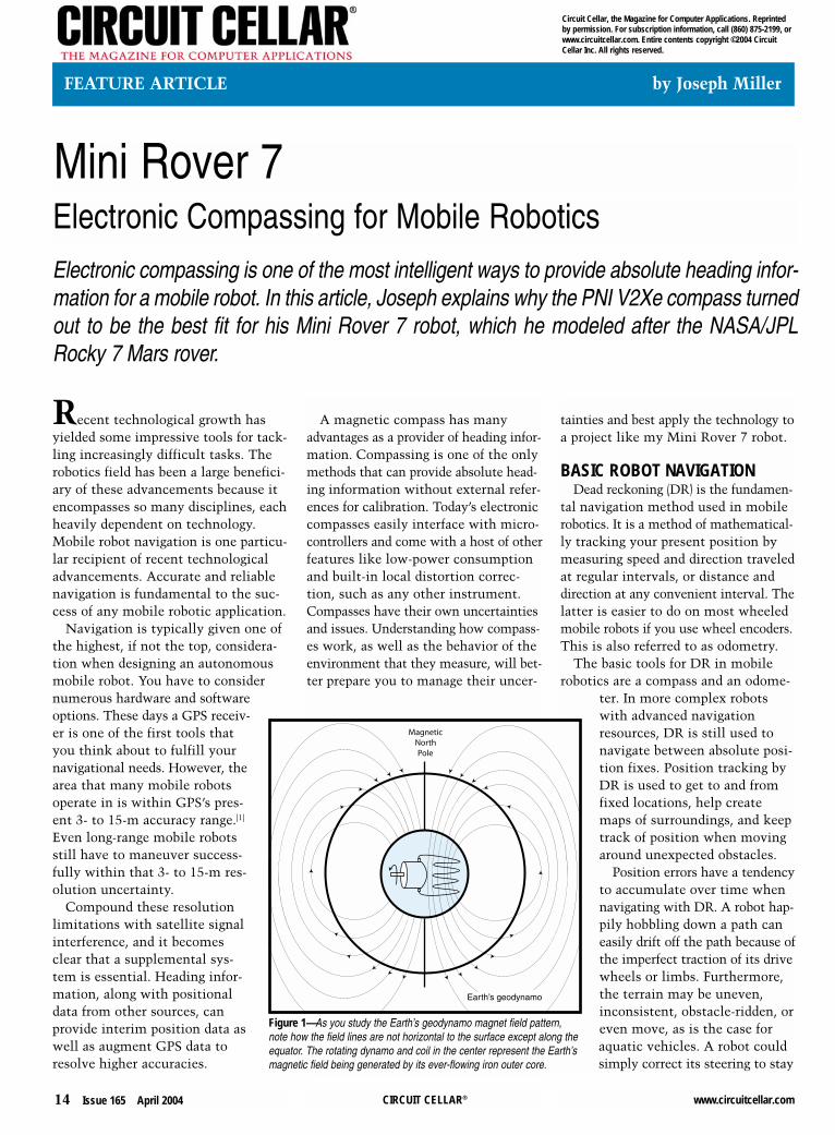
Figure 1—As you study the Earth’s geodynamo magnet field pattern,note how the field lines are not horizontal to the surface except along theequator. The rotating dynamo and coil in the center represent the Earth’smagnetic field being generated by its ever-flowing iron outer core.
www.circuitcellar.com CIRCUIT CELLAR® Issue 165 April 2004 15
model of the system with the statisticalbehavior of system errors. It enables nav-igation systems to handle periodic GPSsignal interruption, odometer slippage,magnetic anomalies, and other sensorirregularities with minimal degradationof accuracy. Kalman filters also can beextremely complicated. You must fullyunderstand the dynamic behavior of yoursystems and the statistical and systemicerrors of your sensors in order to makeproper use of Kalman filters. It might beeasier and more feasible in less demand-ing projects to use other software-basedanalytical tools like averaging, weightedaveraging, limiting, and majority votingto improve heading data reliability.
MAGNETIC COMPASSINGThe Earth’s magnetic field is created
deep in its iron core by a regenerativemagnetic field generator that’s some-times referred to as the geodynamo. Thisiron core has a liquid outer section and asolid inner section. The flow of electri-cal current in the turbulent liquid ironouter section creates the magnetic field.
The simplest description of the Earth’smagnetic field spatial pattern is that of adipolar field with magnetic flux emanat-ing from the South Pole and convergingat the North Pole. The Earth’s magneticfield pattern is a little more complexthan a simple bar magnet model. As pre-viously mentioned, the Earth’s geody-namo is constantly moving. Presently,the magnetic poles are tilted about 11°away from the geographical poles, andthey are not at exactly at opposite sidesof the world either. The magnetic NorthPole is located in northeastern Canada,and the magnetic South Pole is located inthe Antarctic Ocean south of Australia.
The geographical North Pole is alsoknown as true north. The angular dif-ference between the true poles and themagnetic poles at a given location iscalled the declination angle. Dependingon your location, true north couldappear to either the east or west of themagnetic North Pole.
The Earth’s spherically shaped geo-dynamo produces a magnetic field asshown in Figure 1. Note that the fieldlines are not horizontal to the Earth’ssurface, except at the Earth’s magneticequator. Unlike the Earth’s straightgeographical equator, this one mean-
on course (or on bearing), but that littleoff-course excursion could add a smallposition error. The magnitude of theposition error is the integral of time,distance, and off-course angle traveledwhile the robot is off course. What isreally required is a new bearing calcu-lation to increase the robot’s chancesto reach the desired target.
HEADING DETERMINATIONFor centuries, we have been taking
advantage of the Earth’s magnetic field toorient ourselves with respect to its mag-netic poles. Both the mechanical needlecompass and electronic compass canprovide absolute heading information. Itis hard to beat the compass for this pur-pose. With the exception of GPS, othersystems that exist require an externalheading reference as calibration.
Gyroscopes use mechanical angularmomentum changes to measure angu-lar and linear movements. Traditionalflywheel gyroscopes are fast-spinninggimbaled flywheels with encoders. Theencoders are situated about the pivotalaxes of the gyroscope’s gimbals and reg-ister angular movement of the spatiallystable flywheels to its base, which isfastened to a host vessel. Modern gyro-scopes use micro electromechanicalsystems (MEMS) and optical technolo-gies in place of the bulky flywheels.
Gyroscopes have fast response timesand are insensitive to magnetic anom-alies. They are also relative angularposition sensors, which require anexternal reference heading to initiallyset. A special kind of gyroscope calledthe gyrocompass can align itself withthe Earth’s rotational axis, but it tendsto be a large and costly instrument.
Differential wheel encoding is anothertechnique used to determine heading.Relative heading changes can be comput-ed by taking the difference of distancetraveled by two opposing wheels. Thistechnique has the same traction and ter-rain issues associated with the aforemen-tioned wheel encoder odometry.
A single-antenna GPS can provideheading information, but it is not instan-taneous. It inherently lags the movementof the robot or vehicle because the derivedheading requires previous position data. AGPS could not tell you where you areheading if you were to stop and changedirections. Like compasses, GPS receiversdo not require external reference headingcalibration. Once moving, the GPS head-ing update rate is a maximum of approxi-mately 1 Hz, although some receivers adddamping, which increases this time con-stant even more. A dual-antenna GPSreceiver can provide instantaneous head-ing—or yaw—information, although therecommended distance between the twoantennas is 1 m. This fact, along with itslarge price tag, can be a limiting factorfor many mobile robot applications.
A combination of techniques is thebest approach. There are many ways todetermine heading, each of which hasits own strengths and weaknesses. Noneof them are infallible. For this reason,some systems use two or more methodscooperatively to increase system accura-cy and reliability. The deciding factorsare cost, accuracy, efficiency, features,availability, ease of use, speed, and size.
Kalman filters are typically used tointegrate the data from multiple sensorsto produce a more reliable and accurateheading. Kalman filtering is a statisticalmethod that combines the dynamic
Figure 2—I plotted the magnetometer sensor output versus the angle. You can also see the x-y plot of the magne-tometer sensor output.
16 Issue 165 April 2004 CIRCUIT CELLAR® www.circuitcellar.com
components, a horizontal componentand a vertical component. At the mag-netic equator where the magnetic fieldis horizontal, the field has no verticalcomponent. At the magnetic poles, thefield is purely vertical and has no hori-zontal component. At places where theinclination angle is 45°, the horizontaland vertical components are equal.
The U.S. Geological Service (USGS)and the Nation Oceanic and AtmosphereAdministration (NOAA) maintain websites that have global maps and on-line
ders but is located in roughly the samearea. At the magnetic poles, the fieldlines are vertical. The angular vector ofthe magnetic field with respect to thehorizontal plane at any given locationis known as the dip angle, or inclina-tion angle. The density of the magnet-ic field also varies around the world.The magnetic field density is approxi-mately two times as dense at the mag-netic poles as it is at the equator.
The magnetic field vector is some-times referred to as having two separate
programs that chart declination angles,field intensities, dip angles, and muchmore. I will focus on the horizontal com-ponent of the magnetic field, becausethat is the portion that contains the head-ing information that I wish to measure.
MAGNETIC MEASUREMENTSA magnetometer is an instrument that
can measure the flux density of a mag-netic field. It uses one of any number oftypes of sensors to convert magnetic fluxto voltage, current, frequency, or someother electronically measurable form.
There are numerous types of magnet-ic field sensors: the saturable core mag-netometer (or fluxgate magnetometer),the Hall effect sensor, the magneto-resistive sensor, and the magneto-inductive sensor. A two-axis magne-tometer, in which the two sensors arein quadrature (orthogonal) orientation,can be used as an electronic compass tocompute heading. When it is parallelwith the measured field, the magne-tometer sensor’s output is at maximumfor the given amount of magnetic fluxdensity that is present. When the mag-netometer sensor is perpendicular tothe magnetic lines of flux, the sensorwill output no signal. A plot of the x-sensor output versus the y-sensor out-put results in the heading being repre-sented around the polar axis of thecoordinate system origin (see Figure 2).
This form is preferred as a visual analy-sis tool for sensor and system perform-ance analysis and troubleshooting. Noticethat the y-axis is inverted from that of atypical Cartesian coordinate system. Thiswas done so that the compass coordi-nates would be produced in its correctorientation. When operating with com-pass coordinates, it is important toremember to make the proper transla-tions from a Cartesian coordinate systemto a compass coordinate system, especial-ly after using trigonometric functions.
At angles between parallel andantiparallel with respect to the mag-netic lines of flux, the sensor’s outputsignal, X, is a product of the appliedmagnetic flux density, β, and thecosine of the angle, θ, of the sensorfrom being parallel with the flux lines.
[1]
If a second sensor is added, and if it is
X = β θcos( )
www.circuitcellar.com CIRCUIT CELLAR® Issue 165 April 2004 17
ances. There are permanent magnetsin your robot’s motors, and there ismagnetized metal in the robot’s con-struction materials.
positioned at a right angle to the first sen-sor, its output, Y, will have the samefunction as X, but will be 90° out ofphase. The y sensor will be in the eastposition, and the x sensor will be in thenorth position. The two sensors are saidto be in quadrature with one another. Theequation for output Y is the following:
[2]
You now have enough data to com-pute heading from the output valuesof the x and y sensors. Use thetrigonometric identity:
[3]
Combining Equations 1–3 yields:
[4]
The arctangent, or inverse tangent(tan–1), is inherently restricted to ±90°,which covers only two quadrants ofthe coordinate system over its entireinput range of –∞ to ∞. This functionalso operates in the Cartesian coordi-nate system, which is rotated 90° fromcompass coordinates.
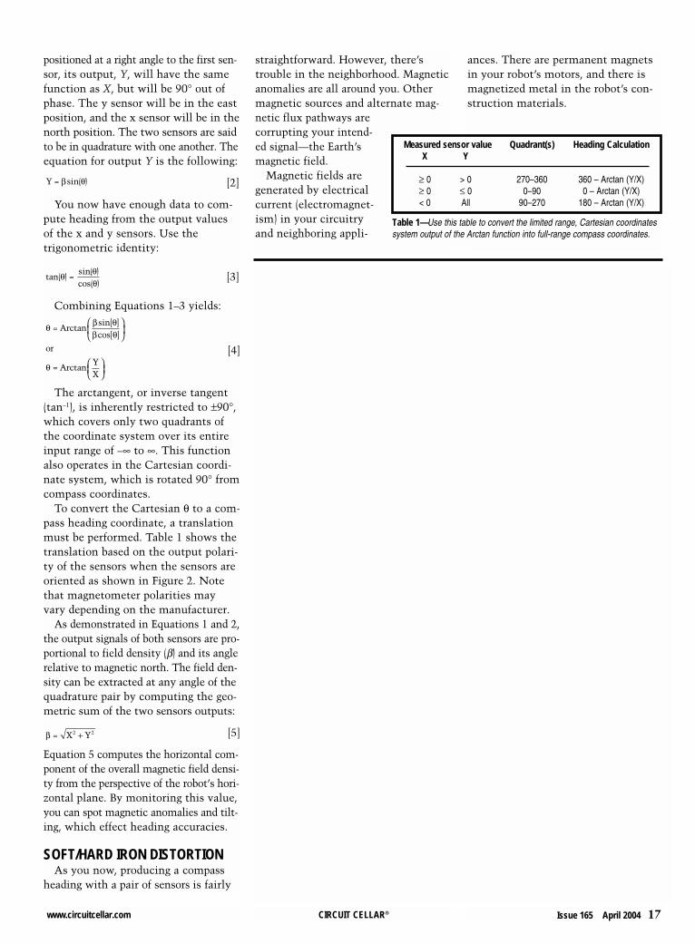
To convert the Cartesian θ to a com-pass heading coordinate, a translationmust be performed. Table 1 shows thetranslation based on the output polari-ty of the sensors when the sensors areoriented as shown in Figure 2. Notethat magnetometer polarities mayvary depending on the manufacturer.
As demonstrated in Equations 1 and 2,the output signals of both sensors are pro-portional to field density (β) and its anglerelative to magnetic north. The field den-sity can be extracted at any angle of thequadrature pair by computing the geo-metric sum of the two sensors outputs:
[5]
Equation 5 computes the horizontal com-ponent of the overall magnetic field densi-ty from the perspective of the robot’s hori-zontal plane. By monitoring this value,you can spot magnetic anomalies and tilt-ing, which effect heading accuracies.
SOFT/HARD IRON DISTORTIONAs you now, producing a compass
heading with a pair of sensors is fairly
β = X Y2 2+
θ β θβ θ
θ
= Arctan
= Arctan
sin[ ]cos[ ]
or
YX
tan( )sin( )cos( )
θ θθ
=
Y = β θsin( )
straightforward. However, there’strouble in the neighborhood. Magneticanomalies are all around you. Othermagnetic sources and alternate mag-netic flux pathways arecorrupting your intend-ed signal—the Earth’smagnetic field.
Magnetic fields aregenerated by electricalcurrent (electromagnet-ism) in your circuitryand neighboring appli-
Measured sensor value Quadrant(s) Heading CalculationX Y
Table 1—Use this table to convert the limited range, Cartesian coordinatessystem output of the Arctan function into full-range compass coordinates.
18 Issue 165 April 2004 CIRCUIT CELLAR® www.circuitcellar.com
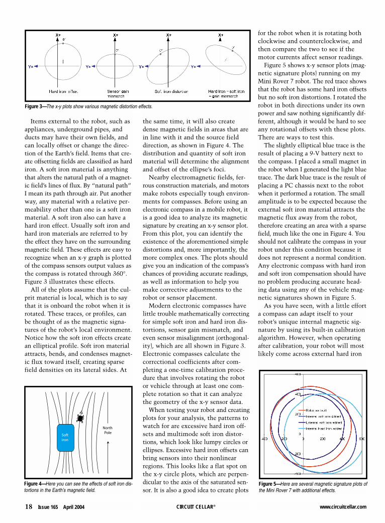
Items external to the robot, such asappliances, underground pipes, andducts may have their own fields, andcan locally offset or change the direc-tion of the Earth’s field. Items that cre-ate offsetting fields are classified as hardiron. A soft iron material is anythingthat alters the natural path of a magnet-ic field’s lines of flux. By “natural path”I mean its path through air. Put anotherway, any material with a relative per-meability other than one is a soft ironmaterial. A soft iron also can have ahard iron effect. Usually soft iron andhard iron materials are referred to bythe effect they have on the surroundingmagnetic field. These effects are easy torecognize when an x-y graph is plottedof the compass sensors output values asthe compass is rotated through 360°.Figure 3 illustrates these effects.
All of the plots assume that the cul-prit material is local, which is to saythat it is onboard the robot when it isrotated. These traces, or profiles, canbe thought of as the magnetic signa-tures of the robot’s local environment.Notice how the soft iron effects createan elliptical profile. Soft iron materialattracts, bends, and condenses magnet-ic flux toward itself, creating sparsefield densities on its lateral sides. At
the same time, it will also createdense magnetic fields in areas that arein line with it and the source fielddirection, as shown in Figure 4. Thedistribution and quantity of soft ironmaterial will determine the alignmentand offset of the ellipse’s foci.
Nearby electromagnetic fields, fer-rous construction materials, and motorsmake robots especially tough environ-ments for compasses. Before using anelectronic compass in a mobile robot, itis a good idea to analyze its magneticsignature by creating an x-y sensor plot.From this plot, you can identify theexistence of the aforementioned simpledistortions and, more importantly, themore complex ones. The plots shouldgive you an indication of the compass’schances of providing accurate readings,as well as information to help youmake corrective adjustments to therobot or sensor placement.
Modern electronic compasses havelittle trouble mathematically correctingfor simple soft iron and hard iron dis-tortions, sensor gain mismatch, andeven sensor misalignment (orthogonal-ity), which are all shown in Figure 3.Electronic compasses calculate thecorrectional coefficients after com-pleting a one-time calibration proce-dure that involves rotating the robotor vehicle through at least one com-plete rotation so that it can analyzethe geometry of the x-y sensor data.
When testing your robot and creatingplots for your analysis, the patterns towatch for are excessive hard iron off-sets and multimode soft iron distor-tions, which look like lumpy circles orellipses. Excessive hard iron offsets canbring sensors into their nonlinearregions. This looks like a flat spot onthe x-y circle plots, which are perpen-dicular to the axis of the saturated sen-sor. It is also a good idea to create plots
for the robot when it is rotating bothclockwise and counterclockwise, andthen compare the two to see if themotor currents affect sensor readings.
Figure 5 shows x-y sensor plots (mag-netic signature plots) running on myMini Rover 7 robot. The red trace showsthat the robot has some hard iron offsetsbut no soft iron distortions. I rotated therobot in both directions under its ownpower and saw nothing significantly dif-ferent, although it would be hard to seeany rotational offsets with these plots.There are ways to test this.
The slightly elliptical blue trace is theresult of placing a 9-V battery next tothe compass. I placed a small magnet inthe robot when I generated the light bluetrace. The dark blue trace is the result ofplacing a PC chassis next to the robotwhen it performed a rotation. The smallamplitude is to be expected because theexternal soft iron material attracts themagnetic flux away from the robot,therefore creating an area with a sparsefield, much like the one in Figure 4. Youshould not calibrate the compass in yourrobot under this condition because itdoes not represent a normal condition.Any electronic compass with hard ironand soft iron compensation should haveno problem producing accurate head-ing data using any of the vehicle mag-netic signatures shown in Figure 5.
As you have seen, with a little efforta compass can adapt itself to yourrobot’s unique internal magnetic sig-nature by using its built-in calibrationalgorithm. However, when operatingafter calibration, your robot will mostlikely come across external hard iron
North Pole
Softiron
Figure 4—Here you can see the effects of soft iron dis-tortions in the Earth’s magnetic field.
Figure 5—Here are several magnetic signature plots ofthe Mini Rover 7 with additional effects.
Figure 3—The x-y plots show various magnetic distortion effects.
20 Issue 165 April 2004 CIRCUIT CELLAR® www.circuitcellar.com
and soft iron objects, which willalter the Earth’s magnetic fielddirection.
Figure 4 shows how a soft ironobject can alter the heading of arobot as it attempts to keep steady(north in this case) when it movespast the object. Notice that thefield density is sparse in this area.As long as the sensors are relative-ly close (so that they experiencethe same field density ratios), thecompass abilities are not signifi-cantly diminished. This is becausethe heading calculation for a quad-rature sensor pair uses the arctan-gent of the ratio of the two sensors(see Equation 2). The overall fielddensity, or magnitude of the field den-sity, can be monitored by calculatingthe geometric sum of the two sensors(see Equation 4), which can alert youto such anomalies. This informationcan be used to weigh your options.
You may decide to temporarily trustdifferential wheel encoder outputs fortracking heading while the overallmeasured field density falls outsideestablished thresholds. A Kalman fil-ter or your own statistical algorithmcan use this information with othersensor data to make improved esti-mates of actual heading. It is impor-tant to use the compass’s calibrated x-ysensor data to compute field densitybecause it already has been compen-sated for your robot’s personal mag-netic signature. Modern electroniccompasses like the PNI V2Xe canreport the overall field density in pro-portion to the field that it experiencedat every heading angle during a cali-bration cycle so that local field distor-tions do not interfere with the assess-ment of external magnetic fields.
EFFECTS OF TILTTilting an electronic compass can
create heading errors. When tilted, thesensors no longer receive the magnet-ic field in the proportions measuredduring calibration. Equations 1 and 2characterize the sensor output valuewith respect to the magnetic field’sangle to the sensor’s orientation in thehorizontal plane. Tilting the sensorwould expose the sensor to portions ofthe Earth’s vertical field component
and reduce its exposure to the hori-zontal field component, which couldeither be an increase or decrease in fielddensity depending on local inclinationangles and direction of tilt.
Equation 6 gives the relationship ofheading error versus tilt angle when acompass is tilted in the north-southrotational axis (also known as pitch):
[6]
where θERR is the heading error causedby tilt, α is the pitch angle compass,and ϕ is the inclination angle of theEarth’s magnetic field.
To use an example, if your compasswere located in San Francisco, whichhas a magnetic field inclination angleof 61°, you could expect a heading errorof up to 1.8° for every degree of pitchfor the first 10° of tilt. Tilt in the east-west direction (roll) or any compoundangle of the two tilt axes creates simi-lar errors, although the worst-caseerrors could still be characterized byEquation 6 by simply substituting thepitch angle, α, with a tilt angle in anydirection. Another accuracy-degradingfactor would be the lack of hard ironand soft iron distortion correction inthe pitch and roll axes. The two mostcommon ways to make a compassinsensitive to tilt is to mount a two-axis compass on a gimbal and to use athree-axis, tilt-compensated compass.
COMPASS FEATURESA good compass should have high
dynamic range sensors. The need tocompensate large hard iron offsets is
θ α ϕERR = Arctan sin tan( )
not uncommon, and can accountfor 75% to 90% of the sensor’soperating range. A good compasswill have an operating range that isat least four times the Earth’s mag-netic field density.
A compass also should be able toresolve the Earth’s horizontal mag-netic field component to 1:115 for1° resolution and 1:1146 for 0.1°.These numbers don’t account forsoft iron distortions that effectsensor gains and hard iron offsets,which would increase theserequirements.
A good compass should be tem-perature-compensated. Magneticsensors have temperature dependen-
cies like most sensors. Fortunately, thesensor’s common temperature effectsdrop out of the heading calculationsbecause the arctangent function’sinput value is a ratio of the sensor pair(y/x). Sensor nonlinear temperatureeffects, external hard iron offsets, andsoft iron distortions do not share thistemperature cancellation characteris-tic. Of course, a compass that has hardiron and soft iron compensation isessential. The necessity of tilt com-pensation depends on the robot’srequirements and your budget.
V2Xe COMPASS MODULEI used the V2Xe compass in the Mini
Rover 7 robot. This is a 1″ square elec-tronic compass module that uses anSPI interface as a means of communi-cation. It consumes less than 3 mW ofpower, and has an output resolution of0.01° with a heading accuracy of 2°.Its field measurement range is about20 times that of the Earth’s field,which means that it can operate withextremely large hard iron offsets thatare common in robotic applications.
The V2Xe compass can be calibratedusing one of two methods. Distortion-compensation coefficients along withdeclination settings are stored in non-volatile memory. The V2Xe can pro-vide raw sensor data and compensatedfield magnitude. It has an adjustabledigital low-pass filter for heading.
A continuous calibration is the sim-plest calibration method to performon the V2Xe. Send the calibrationstart command to the V2Xe to begin
Photo 1—No, it isn’t the Spirit rover you’ve seen on the news; it’smy Mini Rover 7 robot.
www.circuitcellar.com CIRCUIT CELLAR® Issue 165 April 2004 21
the calibration process, rotate therobot in one or two complete circles,and then send a calibration stop com-mand to end the calibration process.After completing the calibration, youcan retrieve the heading data from theV2Xe as necessary.
V2Xe IN THE MINI ROVER 7 The Mini Rover 7 depicted in Photo 1
is a working scale model of theNASA/JPL Rocky 7 Mars rover. Itincorporates six drive motors, and ithas a rocker-bogey suspension as wellas a zero turn radius steering systemthat’s capable of rotating the rover inplace. The robot contains a Maxstream900-MHz wireless modem for receiv-ing commands and transmitting datato and from a terminal program on ahost PC, which has a matching wire-less modem.
The Mini Rover 7 also sports aC8051F330 microcontroller that’smounted on a CStamp, which is aBASIC Stamp II socket-compatiblemodule. It contains two regulators anda JTAG programming/debugger portconnector. I used the free integrateddevelopment environment and evalua-tion C compiler supplied by SiliconLaboratories along with its EC2 serial-to-JTAG adapter. The wiring diagramfor the robot is shown in Figure 6.
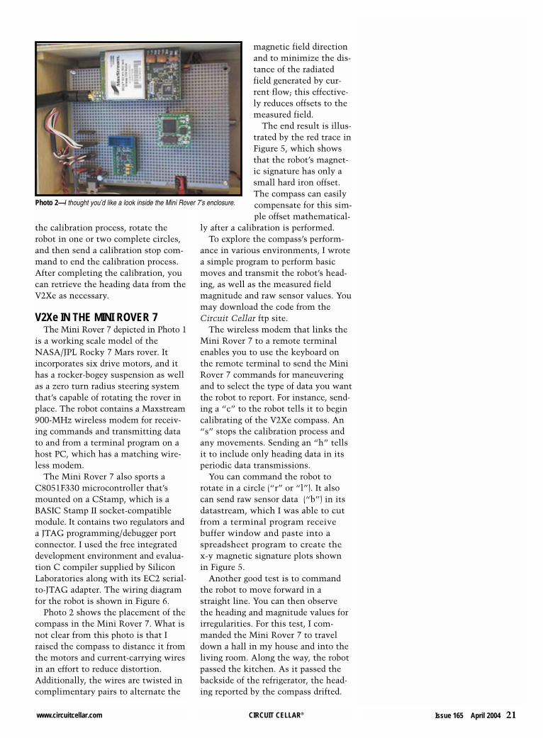
Photo 2 shows the placement of thecompass in the Mini Rover 7. What isnot clear from this photo is that Iraised the compass to distance it fromthe motors and current-carrying wiresin an effort to reduce distortion.Additionally, the wires are twisted incomplimentary pairs to alternate the
magnetic field directionand to minimize the dis-tance of the radiatedfield generated by cur-rent flow; this effective-ly reduces offsets to themeasured field.
The end result is illus-trated by the red trace inFigure 5, which showsthat the robot’s magnet-ic signature has only asmall hard iron offset.The compass can easilycompensate for this sim-ple offset mathematical-
ly after a calibration is performed. To explore the compass’s perform-
ance in various environments, I wrotea simple program to perform basicmoves and transmit the robot’s head-ing, as well as the measured fieldmagnitude and raw sensor values. Youmay download the code from theCircuit Cellar ftp site.
The wireless modem that links theMini Rover 7 to a remote terminalenables you to use the keyboard onthe remote terminal to send the MiniRover 7 commands for maneuveringand to select the type of data you wantthe robot to report. For instance, send-ing a “c” to the robot tells it to begincalibrating of the V2Xe compass. An“s” stops the calibration process andany movements. Sending an “h” tellsit to include only heading data in itsperiodic data transmissions.
You can command the robot torotate in a circle (“r” or “l”). It alsocan send raw sensor data (“b”) in itsdatastream, which I was able to cutfrom a terminal program receivebuffer window and paste into aspreadsheet program to create thex-y magnetic signature plots shownin Figure 5.
Another good test is to commandthe robot to move forward in astraight line. You can then observethe heading and magnitude values forirregularities. For this test, I com-manded the Mini Rover 7 to traveldown a hall in my house and into theliving room. Along the way, the robotpassed the kitchen. As it passed thebackside of the refrigerator, the head-ing reported by the compass drifted.
Photo 2—I thought you’d like a look inside the Mini Rover 7’s enclosure.
that I had observed indoors because Ididn’t encounter manmade iron objects.
THE NEXT MOVEThe program listing posted on the
Circuit Cellar ftp site also contains aPID-based steering control systemthat keeps the robot on a steadycourse—if it doesn’t encounter mag-netic anomalies. The next step for thisproject is to add two wheel encodersto create a differential odometer. Iplan to experiment with this dataalong with compass heading and mag-
nitude information in a weightedaveraging algorithm to increaseheading accuracies. I
22 Issue 165 April 2004 CIRCUIT CELLAR® www.circuitcellar.com
PROJECT FILESTo download the code, go to ftp.circuitcellar.com/pub/Circuit_Cellar/2004/165.
Joseph Miller is a Senior ElectricalEngineer at PNI Corporation,where he designs consumer andOEM sensor- and network-basedproducts. He earned an A.S.E.E.degree from the Heald Institute ofTechnology in San Francisco, andhas been an electrical engineer forapproximately 20 years. Joseph
enjoys competing and demonstrating hisrobots. You may contact him at [email protected].
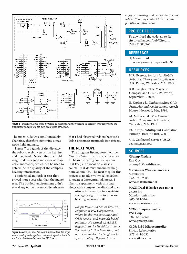
The magnitude was simultaneouslychanging, therefore signifying a mag-netic field anomaly.
Figure 7 is a graph of the distancethe robot traveled versus the headingand magnitude. Notice that the fieldmagnitude is a good indicator of mag-netic anomalies, which can be used todetermine the quality of the compassheading information.
I performed an outdoor test thatproved more successful than the indoortest. The outdoor environment didn’treveal any of the magnetic disturbances
Figure 7—Here you have the robot’s distance from the originversus heading and magnitude during a straight-line test witha soft iron distortion effect near the 125″ mark.
Figure 6—Because I like to make my robots as expandable and serviceable as possible, most subsystems aremodularized and plug into the main board using connectors.