1 Minimum Energy Designs – from Nanostructure Synthesis to Sequential Optimization C. F. Jeff Wu + (joint with Roshan Joseph + & Tirthankar Dasgupta* ) + Georgia Institute of Technology *Harvard University
Transcript
1
Minimum Energy Designs –from Nanostructure Synthesis to Sequential Optimization
C. F. Jeff Wu+
(joint with Roshan Joseph+ & Tirthankar Dasgupta* )
+Georgia Institute of Technology*Harvard University
2
What are Nanostructures?
Functional structures designed from atomic or molecular scale with at least one characteristic dimension measured in nanometers (1 nm = 10-9 meter).
Exhibits novel and significantly improved physical, chemical and biological properties, phenomena and processes.
Building blocks for nano-devices.
Likely to impact many fields ranging from electronics, photonics and optoelectronics to life sciences and healthcare.
3
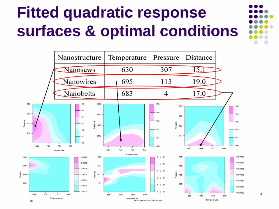
Statistical modeling and analysis for robust synthesis of nanostructures
Dasgupta, Ma, Joseph, Wang and Wu (2008), J. Amer. Stat. Assoc.
Robust conditions for synthesis of Cadmium Selenide (CdSe) nanostructures derived New sequential algorithm for fitting
A 9x5 full factorial experiment was too expensive and time consuming.
Quadratic response surface did not capture nanowire growth satisfactorily (Generalized R2 was 50% for CdSe nanowire sub-model).
6
What makes exploration of optimum difficult? Complete disappearance of morphology in
certain regions leading to large, disconnected, non-convex yield regions.
Multiple optima.
Expensive and time-consuming experimentation 36 hours for each run Gold catalyst required
7
“Actual” contour plot of CdSe nanowire yield Obtained by averaging yields
over different substrates.
Large no-yield (deep green region).
Small no-yield region embedded within yield regions.
Scattered regions of highest yield.
8
How many trials needed to hit the point of maximum yield ?
Pre
ssur
e
Temperature
9
A 5x9 full-factorial experiment
Yield = f(temp, pressure)
17 out of 45 trials wasted (no morphology)!
Pre
ssur
e
10
Why are traditional methods inappropriate ? Need a sequential approach to keep run size to a
minimum. Fractional factorials / orthogonal arrays Large number of runs as number of levels increase. Several no-morphology scenarios possible. Do not facilitate sequential experimentation.
Response Surface Methods Complexity of response surface. Categorical (binary in the extreme case) possible. No clever search algorithm.
11
The Objective To find a design strategy that
Is model-independent, Can “carve out’’ regions of no-morphology
quickly, Allows for exploration of complex response
surfaces, Facilitates sequential experimentation.
12
Pros and Cons of space filling designs LHD (McKay et al. 1979), Uniform designs (Fang
2002) are primarily used for computer experiments.
Can be used to explore complex surfaces with small number of runs.
Model free. Not designed for sequential experimentation. No provision to carve out regions of no-
morphology quickly.
13
Sequential Minimum Energy Designs (SMED)
q1
q2
E = Kq1q2 / d
Charge inversely proportional to yield,e.g., q = 1-yield
Pre
ssur
e
= 0.6
= 1.0
Y = 40%
Y = 0
• Physical connection: treat design points as positively charged particles.
14
What position will a newly introduced particle occupy?
q1
q2
Pre
ssur
e
= 0.6
= 1.0
15
Key idea Pick a point x. Conduct experiment at x and observe yield p(x). Assign charge q(x) inversely proportional to
p(x), e.g., . Use to update your knowledge about
yields at various points in the design space Pick the next point as the one that minimizes
the total potential energy in the design space.
ˆ ( )p x( ) (1 ( ))q x p x γα= −
16
The next design point
17
How the algorithm works
γα )}(1{)( xpxq −=
18
Inverse distance weighting as interpolator Not yet an algorithm, q(x) needs to be “predicted”. Use inverse distance weighting to assign charges to
each yellow point based on yields observed at red (sampled) points:
.
The yellow point that minimizes the potential energy with the four red points, is the next choice.
19
The SMED algorithm( )
11
( )( )
( ) ( )
( )
ˆarg min ( , ),
whereˆ ( ) ( )ˆ ( , ) ,
( , )ˆ ˆ( ) (1 ( )) ,ˆ ( ) : predicted yield at .
nn
n ii
nn i
ii
n n
n
X E x x
q x q xE x xd x x
q x p xp x x
γα
+=
=
=
= −
∑
20
Choice of α Because ,
where .
Lemma 1: For α = 1/pg , if xn = xg for some n = n0,
then xn = xg, for .Once it reaches xg , SMED will stick to the global
optimum (i.e., total energy ).
Undesirable to choose α < 1/pg ; see Theorem 2 later.
( ) (1 ( )) 0q x p x γα= − ≥
1 1[max ( )] ,gxp x pα − −≤ =
x∀
( ) max ( )g g xp p x p x= =
0n n∀ >
1
ˆ ( , ) 0n
iE x x =∑⇒
21
Choice of tuning constants
In practice, pg will not be known. Thus α will be estimated iteratively. First, let’s examine the performance for
deterministic yield functions with fixed α (α = pg
−1) and γ.
22
Performance with known α
)0,0(,0 1 == xγ )0,0(,1 1 == xγ
23
Performance with known α (with different starting points and γ=1)
24
Convergence of SMED
25
Proof (Continued)For any ,
.1),(
11
1
,1
,),(
1),(
.),(
)()(ˆ),(
)()(ˆ
1
12
1
1
1
1
21
1
2
1
1
)1(1
1
)1(
∑
∑
∑∑
∑∑
−
=
−
=
−
=
−
=
−
=∗
∗−−
=
−
≤−
⇒
≤
≥≥
=≤=
i
k nni
n
j
i
k nn
n
j jn
n
j j
jnn
j jn
jnn
dqxxdn
dRHS
xxdq
xxdqLHS
RHSxxd
xqxqxxd
xqxqLHS
ki
i
ki
i
i
i ii
i
i
i
Since is a convergent sequence and , of as , a contradiction. □
}{knx )(iOni = LHS
)(∗
)(∗
∞→ ∞→i
26
Divergence of SMED with wrong α Theorem 2. Under same assumptions, if α<1/pg ,
then is a dense subset of . Proof based on similar ideas. Implications: Smed sequence will visit every part
of the design region, an erratic behavior like the Peano Curve.
The proofs reveal how and work together to move the sequence toward the optima.
)(xq )(xd
27
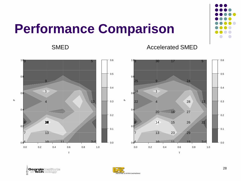
Accelerated SMED For a convergent , its d values → 0. Then the
corresponding q values must also go to 0, i.e., , explaining why α = 1/pg.
By flipping this argument, we can move SMED subsequence quickly out of a region with low q values (i.e., get out of a peak already identified) by redefining the q values for this subsequence to a much higher value. This will force SMED to move quickly out of the region.
}{inx
0)()( =→ gn xqxqi
28
Performance Comparison
0.0
0.1
0.2
0.3
0.4
0.5
0.6
0.0 0.2 0.4 0.6 0.8 1.0
0.0
0.2
0.4
0.6
0.8
1.0
1
2
3
4
5
6
7
8
9
10 11
12
13
1415161718192021222324252627282930
T
P
0.0
0.1
0.2
0.3
0.4
0.5
0.6
0.0 0.2 0.4 0.6 0.8 1.0
0.0
0.2
0.4
0.6
0.8
1.0
1
2
3
4
5
6
7
8
9
10 11
12
13
14 15
16
17
18
19
20
21
22
23
2425
26
27
28
29
30
T
P
SMED Accelerated SMED
29
Criteria for estimator of α
./1 ,/1:tRequiremen
maximum. Global :
iteration,th the tillyield maximum Observed :iteration,th after the of Estimators :
)(
)(
nngn
g
n
n
pp
pnp
n
<→ αα
αα
30
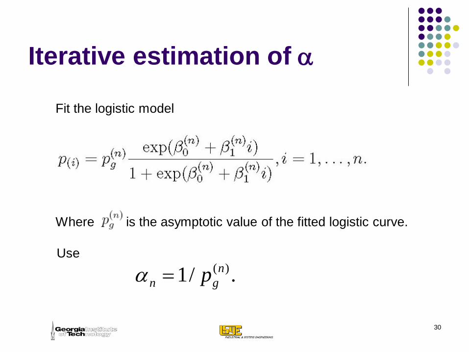
Iterative estimation of α
Fit the logistic model
Where is the asymptotic value of the fitted logistic curve.
./1 )(ngn p=α
Use
31
Some performance measures for n0 - run designs
.
32
Performance evaluation with nanowire yield data
33
Modified Branin function A standard test function in global optimization:
,
has three global minima. To create a large nonconvex and disconnected no-yield
region, use modified Branin function
where
( , ) 0.8( , ) max( ,0),0 , 1,0.2
f u vp u v u v−= ≤ ≤
34
Performance with modified Branin function
35
Performance with modified Branin function (contd.)
36
Random functions
In actual practice the yield function is random.
We actually observe )).(,(~,/)(ˆ xx prbinomialyryp =
37
Performance of usual algorithm with random functions
Result of 100 simulations, starting point = (0,0). Concern: as r decreases, the number of cases in which the global optimum is identified reduces.
38
Improved SMED for random response
Instead of an interpolating function, use a smoothing function to predict yields (and charges) at unobserved points.
Update the charges of selected points as well, using the smoothing function.
Local polynomial smoothing used. Two parameters: nT (threshold number of iterations after which smoothing is
started). λ (smoothing constant; small λ: local fitting).
39
Improved performance with smoothing algorithm, r = 10
40
Summary A new sequential space-filling design SMED
proposed. SMED is model independent, can quickly “carve out”
no-morphology regions and allows for exploration of complex surfaces.
Origination from laws of electrostatics. Some desirable convergence properties. Modified algorithm for random functions. Performance studied using nanowire data, modified
Branin (2 dimensional) and Levy-Montalvo (4 dimensional) functions.
41
Predicting the future
What the hell! I don’t want to use this stupid strategy for experimentation !
Use my SMED !
Image courtesy : www.cartoonstock.com
Nano
Stat
42
43
How many trials? Let’s try one factor at-a-time!
Temperature
Pre
ssur
e
Could not find optimumAlmost 50% trials wasted (no yield)Too few data for statistical modeling
44
Sequential experimentation strategies for global optimization SDO, a grid-search algorithm by Cox and John (1997)
Initial space-filling design. Prediction using Gaussian Process Modeling. Lower bounds on predicted values used for sequential selection
of evaluation points. Jones, Schonlau and Welch (1998)
Similar to SDO. Expected Improvement (EI) Criterion used. Balances the need to exploit the approximating surface with the
need to improve the approximation.
45
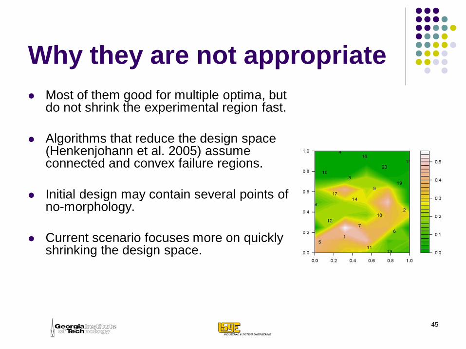
Why they are not appropriate Most of them good for multiple optima, but
do not shrink the experimental region fast.
Algorithms that reduce the design space (Henkenjohann et al. 2005) assume connected and convex failure regions.
Initial design may contain several points of no-morphology.
Current scenario focuses more on quickly shrinking the design space.
46
Performance in higher-dimensions (Levy-Montalvo function)