Minimum Standards for InvestmentPerformance: A New Perspective on Non-Life

Insurer Solvency

Martin Eling, Nadine Gatzert und Hato Schmeiser

Preprint Series: 2009-07

Fakultat fur Mathematik und WirtschaftswissenschaftenUNIVERSITAT ULM

MINIMUM STANDARDS FOR INVESTMENT PERFORMANCE:

A NEW PERSPECTIVE ON NON-LIFE INSURER SOLVENCY

Martin Elinga, Nadine Gatzerta,, Hato Schmeisera

a University of St. Gallen, Institute of Insurance Economics, Kirchlistrasse 2,

9010 St. Gallen, Switzerland

25 March 2009

____________________________________________________________________

Abstract

The aim of this paper is to develop an alternative approach for assessing an insurer’s solvency as a

proposal for a standard model for Solvency II. Instead of deriving minimum capital requirements—as

it is done in solvency regulation—our model provides company-specific minimum standards for risk

and return of investment performance, given the distribution structure of liabilities and a predefined

safety level. The idea behind this approach is that in a situation of weak solvency, an insurer’s asset

allocation can be adjusted much more easily in the short term than can, e.g., claims cost distributions,

operating expenses, or equity capital. Hence, instead of using separate models for capital regulation

and solvency regulation––as is typically done in most insurance markets––our single model will re-

duce complexity and costs for insurers as well as for regulators. In this paper, we first develop the

model framework and second test its applicability using data from a German non-life insurer.

JEL classification: G22; G28; G31

Subject and Insurance Branch Code: IM01; IM20; IE46; IE53; IB50

Keywords: Solvency; Regulation; Investment performance; Non-life insurance; Normal power approx-

imation

____________________________________________________________________

1. INTRODUCTION

Insurance supervision in the European Union is undergoing significant change as the Euro-

pean Commission works toward implementation of new risk-based capital standards (Solven-

cy II). The aim of this paper is to contribute to this discussion by developing a risk model for

the calculation of minimum solvency requirements. Corresponding author. Tel.: +41 71 2434012; fax: +41 71 2434040.

E-mail addresses: martin.eling@unisg.ch, nadine.gatzert@unisg.ch, hato.schmeiser@unisg.ch.

2

We introduce a new perspective on solvency regulation: instead of deriving a minimum

amount of equity capital (as usually done in solvency models), minimum standards for in-

vestment performance are obtained, given the risk structure of liabilities, equity capital, and a

predefined safety level. The functional relationship, which ensures that the minimum safety

standard is met, is denoted as the solvency line. The solvency line determines minimum in-

vestment requirements in terms of expected return and standard deviation of the rate of return

on the insurer’s investment portfolio. In this setting, insurers with higher equity capital will,

ceteris paribus, also have a higher degree of freedom in the choice of their asset allocation.

We compare results when the safety level is derived under three risk measures typically used

in solvency regulation: the ruin probability, tail value at risk, and expected policyholder defi-

cit (see, e.g., Barth, 2000). Having identified risk-return combinations that are compatible

with the solvency rules based on the different risk measures, we further investigate to what

extent these minimum requirements can be met on the capital market using several bench-

mark indices. To illustrate the practicability of the model, we include an empirical application

based on data from a German non-life insurance company.

The literature focuses primarily on the predictability power of existing solvency models, al-

ternative methodologies for solvency analysis, and the economic effects of solvency regula-

tion. To date, empirical tests of solvency models used by regulators are restricted to the Unit-

ed States. Cummins/Harrington/Klein (1995) and Grace/Harrington/Klein (1998), as well as

Cummins/Grace/Phillips (1999), find that the predictive power of the U.S. risk-based capital

standards is relatively low compared to other screening mechanisms based on financial ratios

used by regulators (e.g., the financial analysis tracking system). Pottier/Sommer (2002) con-

clude that the solvency models used by the private sector (A.M. Best ratings) are superior in

predictive ability compared to the measures produced by regulators (risk-based capital stan-

dards, financial analysis tracking system). According to these empirical studies, the predicta-

bility power of the solvency models used by U.S. regulators appears to be limited.1

Consequently, a second stream of literature proposes a number of different methodologies

that can be used to study insolvency and to identify factors explaining insolvencies. Brocket

et al. (1994) use neural networks, Carson/Hoyt (1995) multiple discriminant analysis, Lamm-

Tennant/Starks/Stokes (1996) logistic regressions and a loss cost function, and Baran-

1 The designers of Solvency II are thus able to take advantage of these research results and the con-

sensus therein that neither the European regulatory rules (Solvency I) nor the current regulatory framework in the United States are entirely successful in meeting regulatory objectives. Further-more, those involved in the Solvency II process can take advantage of advanced computer systems capable of implementing more complex models. Hence, differences in solvency systems may par-tially be explained by the different states of knowledge extant when they were first introduced.

3

off/Sager/Witt (1999) cascaded logistic regressions. An overview of these methods is pro-

vided in Carson/Hoyt (2000) as well as in Chen/Wong (2004). An important aspect in the

discussion of alternative methodologies is the use of different risk measures, such as the ruin

probability or the tail value at risk (see, e.g., Butsic, 1994; Barth, 2000; Tasche, 2002; Cuo-

co/Hong, 2006).

Several authors discuss the economic effects of regulation on insurance markets, often focus-

ing on different forms of regulation and on different sectors of the insurance industry. Gra-

bowski/Kip Viscusi/Evans (1989), for instance, focus on rate regulation in auto insurance,

Barros (1995) analyzes market entry regulation in auto insurance, and Zwei-

fel/Telser/Vaterlaus (2006) study product regulation in health insurance. With a focus on sol-

vency regulation, Munch and Smallwood (1980) find that minimum capital requirements re-

duce the number of insolvencies by reducing the number of small firms; they conclude that

capital requirements are a particular burden for small insurers. Recent literature also high-

lights the particularly strong effect of regulation on small insurers (see, e.g., Van Rossum,

2005, on the interrelation between degree of regulation and corresponding costs).

Rees/Gravelle/Wambach (1999) show that insurers always provide enough capital to ensure

solvency if consumers are fully informed of insolvency risk; they conclude that regulators

should provide information rather than imposing capital requirements. While most studies

argue against extensive solvency regulation, this issue is not our main concern; instead we

consider solvency regulation as a given component of insurance markets.

An overview of the new Solvency II regulation is provided by Eling/Schmeiser/Schmit

(2007), Steffen (2008), and Doff (2008). Currently, a framework directive by the European

Commission (2008) is under discussion and quantitative impact studies are being conducted.

The final draft of the directive should be submitted for resolution by the EU parliament in

2009 and Solvency II should become the general norm by 2012. In the context of Solvency II,

different aspects of harmonization are discussed, such as the convergence of Solvency II and

International Financial Reporting Standards (see Esson/Cooke, 2007) or the convergence of

solvency regulation around the world (see Karp, 2007; Monkiewicz, 2007). One of Solvency

II’s innovations is that it allows an insurer to use internal risk models instead of standardized

risk models when determining target capital (i.e., the minimum capital an insurer needs for a

given time horizon and a fixed safety level). An internal model is constructed by the insurer

for its individual needs; a standard model is designed by the regulator and used uniformly

across insurers. Liebwein (2006) discusses some requirements for Solvency II internal risk

models. Schmeiser (2004) develops an internal risk model for property-liability insurers based

on dynamic financial analysis. Only a few approaches and aspects of a standard model under

4

Solvency II have been discussed at present (see, e.g., Sandström, 2006, for fundamental mod-

eling ideas, or Schubert and Grießmann, 2007, for the “German” approach). The current

framework directive already contains a number of principles and a target capital formula, but

the precise implementation is unsettled as yet (see European Commission, 2008).

There are two potential problems with the target capital concept as laid out in Solvency II.

First, a common assumption in this calculation is that the insurer’s asset structure remains

unchanged in the time period under review, which is rather unrealistic in practice since the

risk structure can change substantially in the short term. It seems more reasonable to assume

that the liabilities change only marginally in the medium term. Second, in states of weak sol-

vency, raising additional equity capital or implementing other risk management measures will

be difficult. In such a situation, an insurer’s asset allocation can be adjusted much more easily

in the short term operative business than can the claims costs distribution, operating expenses,

or equity capital. We argue that the insurer’s solvency situation should be assessed by esti-

mating the risk structure of liabilities and the available equity capital. Then, based on these

data, the asset structure should be regulated, rather than requiring a certain minimum amount

of capital.

A further problem related to solvency assessment is that developing theoretically sound inter-

nal risk models is expensive and is generally only feasible for large insurance companies with

sufficient financial and technical resources. Most insurers will need to use a preset standard

model to calculate their target capital. To this end, we believe that the model presented in this

paper will prove advantageous compared to existing standard approaches. First, and as shown

in the following sections, it is easy to communicate and simple to implement. Second, instead

of using separate frameworks, with different scopes and assumptions, to derive capital and

solvency requirements (which is currently how it is done in many states of the United States

as well as in the European Union; see OECD, 2002, Bijapur et al., 2007), our model frame-

work provides an integrated view of the insurer’s risk situation. Third, the approach proposed

in this paper not only provides information relevant to insurance regulators, but can also give

insight and useful advice to insurers themselves regarding corporate risk management deci-

sions.

The remainder of the paper is structured as follows. Section 2 describes the model framework

for determining the solvency line. Section 3 contains an empirical application of the devel-

oped standard model using data of a German property-liability insurer as well as capital mar-

ket data. Section 4 discusses policy implications and Section 5 concludes.

5

2. MODEL FRAMEWORK

In this one-period solvency model, the market value of the insurer’s assets at time t = 0 con-

sists of equity and debt and is denoted by 0A . The debt 0L provided by the policyholders can

be divided into two parts: the net premiums (after reinsurance) paid in t = 0 for contracts writ-

ten in t = 0 (with claim payments to occur after time 0) and net premiums remaining for con-

tracts signed before t = 0 with net claims that are not finally settled in t = 0. The debt corres-

ponds to the market value of the liabilities. The residual between the market value of the as-

sets 0A and liabilities 0L is the insurer’s equity (available) capital 0U .

Analogously, at time t = 1, the equity capital 1U is given by the difference between assets

( 1A ) and liabilities ( 1L ):

1 1 1 0 1 0 0 1 1( )U A L A R L U L R S B . (1)

In Equation (1), 1R r denotes the stochastic rate of return on the insurer’s investment. 1S

stands for the stochastic market value of the net claims after reinsurance in t = 1 for contracts

written in t = 0 or earlier, and 1B are the operating expenses of the insurer in t = 1 (modeled

deterministically).

Given a certain risk measure imposed by a regulatory authority, a required safety level, a

fixed time horizon, and input data for the variables 0L , R , 1S , and 1B , the typical procedure

in standard solvency models is to calculate the minimum (or target) required capital at t = 0.

Whenever the available capital 0U is not sufficient to satisfy the capital requirements, the

insurer may be forced to raise additional equity capital, if this is a feasible option. In a situa-

tion of weak solvency, however, this is usually not easy. Changing the asset allocation so as

to meet the solvency requirements should be much easier to accomplish.

Therefore, the main purpose of this paper is to not calculate minimum capital requirements

for an insurer in t = 0, but to derive minimum performance requirements for the insurer’s in-

vestment portfolio in a E R - R framework, based on a given safety level and a chosen

risk measure. Even though there are other, more complex measures of risk and return that

could be considered, we use E R and R in order to make sure that the model remains

simple to implement in practice.

As an example, consider the ruin probability and a fixed safety level . In this case, the equa-

tion 1 1 10P U P A L must be solved for different values of E R and R ,

6

given the distributional assumptions (see Equation (1)). A comparison of alternative risk

measures, such as ruin probability (RP), expected policyholder deficit (EPD), or tail value at

risk (TVaR), is especially relevant given the debate in the literature over the adequacy of sol-

vency measures (for a discussion of the advantages of the different risk measures see, e.g.,

Barth, 2000).2 To what degree an insurer will have freedom of investment choice will depend

not only on the risk measure and safety level used, but also on the risk structure of its liabili-

ties and the actual equity capital 0U .

For a symmetrically distributed rate of return R and a right-skewed distribution of the claims

S1 (see, e.g., Dickson/Tedesco/Zehnwirth, 1998), one obtains a left-skewed distribution of the

equity capital 1U . In this case, the risk measures listed above generally cannot be calculated

explicitly. In the following analysis, we will apply the normal power approximation for U1

(Daykin/Pentikäinen/Pesonen, 1994, p. 129), which––in contrast to a simulation framework––

allows for analytical expressions of the risk measures.

The basic idea of the normal power approximation is to transform a nonnormally distributed

stochastic variable with nonzero skewness into an auxiliary variable y––using the transforma-

tion v ––in order to make the distribution approximately symmetric and normal. For the equi-

ty capital in t = 1, one thus gets 1y v U , and for the distribution function of 1U , 1G u , it

holds that 1 1G u v u y , where stands for the standard normal distribution

function. Under the normal power approximation, the auxiliary variable y is given by

2 1 11 1 1

1 1

16 9 3

u E Uy v u U U

U U

. (2)

Here, 3 3

1 1 1 1/U E U E U U stands for the skewness of 1U . Alternatively, the

inverse 1v y of the transformation function v results from

2 11 1 1

1

16

u E U Uy y v y

U

.

The first three central moments of 1U are needed for the normal power approximation. Since,

in what follows, we assume that the rate of return is symmetric, we obtain (see Equation (1)):

2 Other risk measures and their use for the calculation of capital requirements have been discussed in

the literature as well. An application of distortion risk measures, e.g., can be found in Wirch and Hardy (1999).

7

1 0 1 1( )E U A E R E S B ;

2 22 21 0 1 0( ) 2 cov ,U A R S A R S ;

3 2

1 1 0 1 1

3220 1 1 1 1

3 ( ) ( )

3 ( ) ( ) .

E U E U A E R E R S E S

A E R E R S E S E S E S

In the following, we apply the normal power concept to three risk measures—the ruin proba-

bility, expected policyholder deficit, and tail value at risk.

Ruin Probability (RP)

The probability of an insolvency at t = 1 is given by

1 1 10RP P U P A L ,

i.e., the probability that the firm’s assets are not sufficient to cover its liabilities. The ruin

probability corresponds to the value at risk approach as planned for Solvency II. For a fixed

ruin probability , use of the normal power approximation for the distribution of 1U leads to

1 10 0P U P v U v .

Since 0v z ( z is the -quantile of the standard normal distribution), the following

equation can be derived using 10 v z :

2

1 1 1 1

10

6

zE U z U U U

, (3)

where z denotes the -quantile of a standard normal distribution. Only when the distribu-

tion of 1U is symmetric, the last term on the right-hand side of Equation (3) becomes zero

and, hence, the normal power approximation merges to a normal approximation.3

3 In general, a left-skewed (right-skewed) distribution for U1 will c.p. imply higher (lower) solvency

requirements.

8

Expected Policyholder Deficit (EPD)

One shortcoming of the ruin probability approach is that it does not take into account the se-

verity of ruin (Butsic, 1994; Powers, 1995). Therefore, other risk measurers have been pro-

posed in the literature and are widely used in insurance practice. For instance, the expected

policyholder deficit (EPD) (Butsic, 1994; Barth, 2000) is, in the present context, defined as

1max 0 ,0EPD E U ,

i.e., the expected loss in the case of insolvency, if the equity capital at time 1 becomes nega-

tive. The expected policyholder deficit (EPD) can be written as

1 1 1max 0 ,0 max ,0EPD E U E U E U .

For 0,1Y N , where is the cumulative distribution function of the standard normal

distribution and stands for the respective density function, it holds that (see Wink-

ler/Roodman/Britney, 1972)

0

0 0

vn n n nv v

E Y y y dy E Y E Y

,

where, in general,

1 21z n n z nE Y z z n E Y

0zE Y z

1zE Y z .

Using this result and the normal power approximation for the distribution of 1U ,

1max ,0E U can be derived from the relationship

9

11 1 1 10 0

21 11 10

1 11 10 0

21 1

0

01 11 10 0

21 10

1 11

max ,0

16

6

6

6

6

6

v

v

v v

v

v v

v

E U u g u du v y y dy

U UE U U y y y dy

U UE U y dy U y y dy

U Uy y dy

U UE U E Y U E Y

U UE Y

U UE U

1

1 1

1 11 1

0 0

1 0 0 06

0 0 0 .6

v U v

U Uv v v

U UE U v U v v

Thus, the expected policyholder deficit is given by

1 11 10 0 0

6

U UEPD E U v U v v

, (4)

where v is given by Equation (2).

Tail Value at Risk (TVaR)

Another common risk measure in the insurance sector is tail value at risk (Artzner et al.,

1999) as implemented in the Swiss Solvency Test. Using the value at risk VaR for a safety

level ,

1VaR U q ,

the tail value at risk (TVaR ) for the safety level is given by the conditional expectation:

10

1 1 1¦TVaR U E U U q .

If the normal power approximation to estimate the distribution of 1U is used, the tail value at

risk can be derived analytically by

1 1 1 1

1 1 1

1

1

1 11 1

¦

¦ ¦

max ,0

6.

TVaR U E U U VaR U

E q U U q E q U q

E q Uq

P U q

U UE U v q U v q v q

(5)

using the result for the EPD.

To derive minimum requirements for the insurer’s investment performance in an E R -

R relationship, we fix the company’s safety level using the discussed risk measurers.

Equations (3), (4), and (5) are then solved for E R for a given R . In practical applica-

tions, the minimum required safety level is set by the regulatory authority. In case of the EPD

or TVaR, the requirements are often defined as a percentage of the business volume so as to

ensure comparability between companies of different size.

3. NUMERICAL EXAMPLE BASED ON EMPIRICAL DATA

To illustrate the applicability of the model, we obtained data from a representative medium-

sized German non-life insurance company that mainly deals in property-casualty and automo-

bile insurance. To protect the anonymity of the company, we transformed all data so as to

change the absolute values but not the underlying risk structure.

The market value of the assets in t = 0, 0A , is € 1.582 billion. We derived the stochastic mar-

ket value of net claims in t = 1 with an expected value 1E S of € 1.171 billion and a stan-

dard deviation 1S of € 66 million. The skewness of the claims, 1S , is 0.3. The operat-

ing expenses of the insurer ( 1B , modeled deterministically) yield € 246 million.4 In the nu-

4 The market value of the company’s liabilities in t is given as the sum of the market value of the net

claims and the operating expenses of the insurer. One way to determine the market value of the lia-

11

merical example we assume stochastic independence between the rate of return of the invest-

ment portfolio and the claim payments. The skewness of the equity capital in t = 1, 1U , is then

given by (Daykin et al., 1994, p. 25)

3 3

0 1 11 3 / 22 2

0 1

A R R S SU

A R S

.

The skewness 1U is needed for deriving the different risk measures presented in Equa-

tions (3), (4), and (5).

Given a certain safety level for an insurance company and the data above, requirements for

the investment performance in a E R - R framework can be derived that should be met

at any time between t = 0 and t = 1 (that is, e.g., after any change in the insurer’s asset alloca-

tion).

Comparison of Solvency Lines for Different Risk Measures

In accordance with the planned Solvency II rules (see European Commission, 2008, Article

101), the ruin probability RP is set to = 0.5%. For the TVaR, we use a safety level of =

1% as is also done, e.g., in the Swiss Solvency Test (see Luder, 2005). In the following, we

refer to r instead of R (= 1 + r) for clarity of exposition. To have the same starting value

1E r E R for all three risk measures given 0r R and to thus ensure

comparability, we set 1% 1TVaR U = € 7.827 million and EPD = € 0.135 million. Figure 1

presents the resulting solvency lines for RP, TVaR, and EPD.

bilities caused by contracts sold by the insurer before t = 1 (without new business) is using risk-neutral valuation, as described by the following expression:

1 11 1 1 1

1 1

f fr t r tQ

t t

L S B E S t e B t e

.

Here, fr stands for the risk-free rate of return (here assumed to be constant in time) and 1 .QE

denotes the conditional expected value with respect to the risk-neutral measure Q given the infor-mation available in t = 1 (see, e.g., Björk, 2004). Thus, from the viewpoint of t = 0, the liabilities in t = 1 are stochastic. In our numerical example, the stochastic market value of net claims and the market value of assets have been estimated by the German non-life insurance company.

12

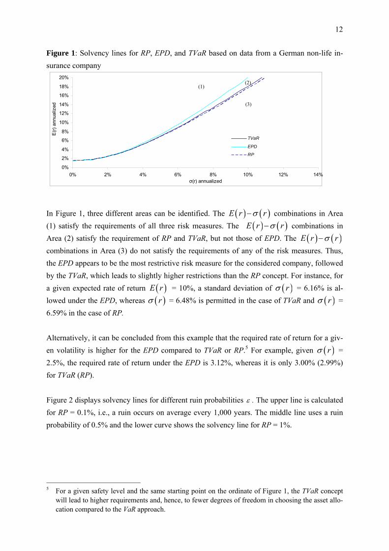
Figure 1: Solvency lines for RP, EPD, and TVaR based on data from a German non-life in-

surance company

0%

2%

4%

6%

8%

10%

12%

14%

16%

18%

20%

0% 2% 4% 6% 8% 10% 12% 14%σ(r) annualized

E(r

) an

nual

ized

TVaR

EPD

RP

In Figure 1, three different areas can be identified. The E r r combinations in Area

(1) satisfy the requirements of all three risk measures. The E r r combinations in

Area (2) satisfy the requirement of RP and TVaR, but not those of EPD. The E r r

combinations in Area (3) do not satisfy the requirements of any of the risk measures. Thus,

the EPD appears to be the most restrictive risk measure for the considered company, followed

by the TVaR, which leads to slightly higher restrictions than the RP concept. For instance, for

a given expected rate of return E r = 10%, a standard deviation of r = 6.16% is al-

lowed under the EPD, whereas r = 6.48% is permitted in the case of TVaR and r =

6.59% in the case of RP.

Alternatively, it can be concluded from this example that the required rate of return for a giv-

en volatility is higher for the EPD compared to TVaR or RP.5 For example, given r =

2.5%, the required rate of return under the EPD is 3.12%, whereas it is only 3.00% (2.99%)

for TVaR (RP).

Figure 2 displays solvency lines for different ruin probabilities . The upper line is calculated

for RP = 0.1%, i.e., a ruin occurs on average every 1,000 years. The middle line uses a ruin

probability of 0.5% and the lower curve shows the solvency line for RP = 1%.

5 For a given safety level and the same starting point on the ordinate of Figure 1, the TVaR concept

will lead to higher requirements and, hence, to fewer degrees of freedom in choosing the asset allo-cation compared to the VaR approach.

(1) (2)

(3)

13

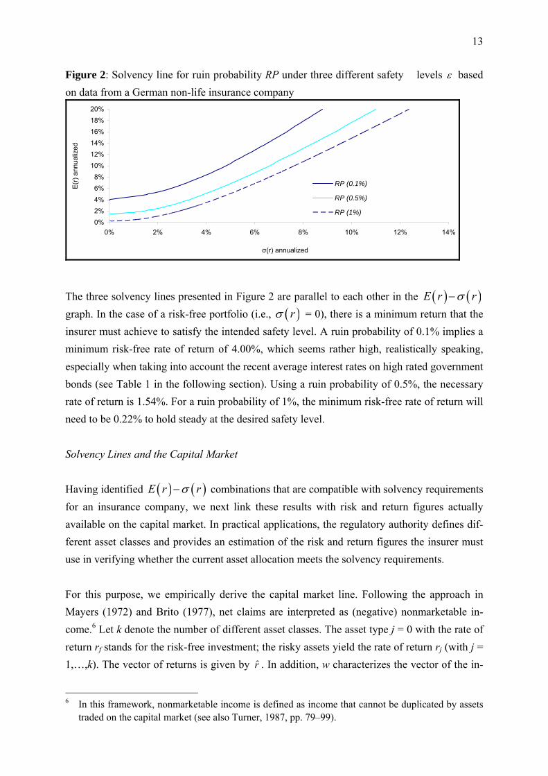
Figure 2: Solvency line for ruin probability RP under three different safety levels based

on data from a German non-life insurance company

0%

2%

4%

6%

8%

10%

12%

14%

16%

18%

20%

0% 2% 4% 6% 8% 10% 12% 14%

σ(r) annualized

E(r

) an

nual

ized

RP (0.1%)

RP (0.5%)

RP (1%)

The three solvency lines presented in Figure 2 are parallel to each other in the E r r

graph. In the case of a risk-free portfolio (i.e., r = 0), there is a minimum return that the

insurer must achieve to satisfy the intended safety level. A ruin probability of 0.1% implies a

minimum risk-free rate of return of 4.00%, which seems rather high, realistically speaking,

especially when taking into account the recent average interest rates on high rated government

bonds (see Table 1 in the following section). Using a ruin probability of 0.5%, the necessary

rate of return is 1.54%. For a ruin probability of 1%, the minimum risk-free rate of return will

need to be 0.22% to hold steady at the desired safety level.

Solvency Lines and the Capital Market

Having identified E r r combinations that are compatible with solvency requirements

for an insurance company, we next link these results with risk and return figures actually

available on the capital market. In practical applications, the regulatory authority defines dif-

ferent asset classes and provides an estimation of the risk and return figures the insurer must

use in verifying whether the current asset allocation meets the solvency requirements.

For this purpose, we empirically derive the capital market line. Following the approach in

Mayers (1972) and Brito (1977), net claims are interpreted as (negative) nonmarketable in-

come.6 Let k denote the number of different asset classes. The asset type j = 0 with the rate of

return rf stands for the risk-free investment; the risky assets yield the rate of return rj (with j =

1,…,k). The vector of returns is given by r . In addition, w characterizes the vector of the in-

6 In this framework, nonmarketable income is defined as income that cannot be duplicated by assets

traded on the capital market (see also Turner, 1987, pp. 79–99).

14

vestment proportions in the different asset classes, the superscript T denotes the transposition

of a vector, and C stands for the covariance matrix of the returns of the different asset classes.

The optimization problem is then described by:

2 221 0 1 0 1ˆ2 cov , minT T

wU A w C w S A w r S

such that

1 0 1ˆ1 .TE U A w E r E S B const

1 1T w .

For the optimal vector w derived by the optimization, one obtains efficient risk–return combi-

nations for ˆTE r w E r and 2 Tr w C w .7

The estimated capital market line is based on benchmark indices that represent investment

opportunities available. German insurers typically hold a globally diversified portfolio of

stocks, bonds, real estate, and money market instruments (these four asset classes cover ap-

proximately 99.50% of all investments made by insurance companies; see El-

ing/Schuhmacher, 2007). Within these four asset classes, we consider 11 indices, each having

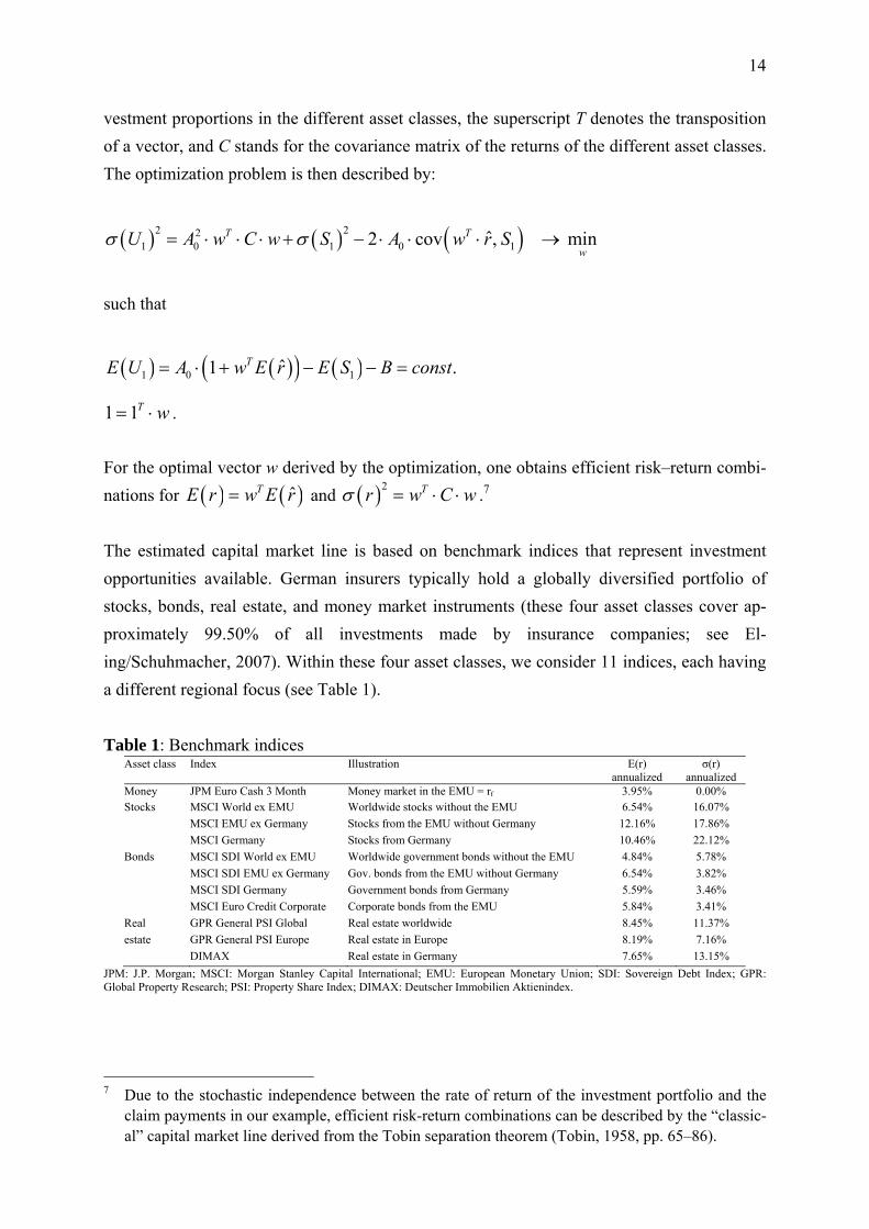
a different regional focus (see Table 1).

Table 1: Benchmark indices Asset class Index Illustration E(r)

annualized σ(r)

annualizedMoney JPM Euro Cash 3 Month Money market in the EMU = rf 3.95% 0.00% Stocks MSCI World ex EMU Worldwide stocks without the EMU 6.54% 16.07%

MSCI EMU ex Germany Stocks from the EMU without Germany 12.16% 17.86%

MSCI Germany Stocks from Germany 10.46% 22.12%

Bonds MSCI SDI World ex EMU Worldwide government bonds without the EMU 4.84% 5.78%

MSCI SDI EMU ex Germany Gov. bonds from the EMU without Germany 6.54% 3.82%

MSCI SDI Germany Government bonds from Germany 5.59% 3.46%

MSCI Euro Credit Corporate Corporate bonds from the EMU 5.84% 3.41%

Real GPR General PSI Global Real estate worldwide 8.45% 11.37%

estate GPR General PSI Europe Real estate in Europe 8.19% 7.16%

DIMAX Real estate in Germany 7.65% 13.15%

JPM: J.P. Morgan; MSCI: Morgan Stanley Capital International; EMU: European Monetary Union; SDI: Sovereign Debt Index; GPR: Global Property Research; PSI: Property Share Index; DIMAX: Deutscher Immobilien Aktienindex.

7 Due to the stochastic independence between the rate of return of the investment portfolio and the

claim payments in our example, efficient risk-return combinations can be described by the “classic-al” capital market line derived from the Tobin separation theorem (Tobin, 1958, pp. 65–86).

15

The selected market indices are well known and can usually be acquired over index funds

with small transaction costs. Furthermore, they are broadly diversified so that they are gener-

ally well suited for performance measurement (for criteria appropriate for selecting represent-

ative benchmark indices, see, e.g., Sharpe, 1992). For each of these indices, we extract

monthly returns between January 1994 and December 2006 from the Datastream database and

calculate mean and standard deviation of the annualized returns. To consider returns from

changes in prices and dividend payments, we look at performance indices only. All indices

are calculated on a Euro basis. Based on the returns and their correlation (see Appendix), we

calculate the efficient frontier and the capital market line using the return of the JPM Euro

Cash 3 Month as the risk-free rate (rf = 3.95%). The capital market line resulting from the

optimization problem above is in this case given by

( ) 3.9492 1.0637 ( )E r r .

Figure 3 displays the capital market line along with the solvency lines previously illustrated in

Figure 1.

Figure 3: Capital market line and solvency lines for RP, EPD, and TVaR based on data from

a German non-life insurance company

0%

2%

4%

6%

8%

10%

12%

14%

16%

18%

20%

0% 2% 4% 6% 8% 10% 12% 14%σ(r) annualized

E(r

) an

nual

ized

TVaREPDRPEfficient Frotier

In contrast to Figure 1, which revealed three areas of relevance, Figure 3 shows four different

areas. Looking at Figure 3, we see that risk–return combinations in Areas (1) and (4) comply

with the requirements of the EPD. However, in contrast to the E r r combinations in

Area (4), Area (1) is not attainable on the capital market. Areas (2) and (3) include risk-return

combinations that are only acceptable under RP and TVaR; again, combinations in Area (2)

are not in line with capital market opportunities. Overall, including the capital market line in

Figure 3 reveals the stronger regulatory restriction imposed by the EPD concept, as the al-

(1)

(4)

(2)

(3)

16

lowed standard deviation of the insurer’s investment return is more limited compared to the

other risk measures. In addition, the TVaR concept is more restrictive than the RP for the firm

under consideration.

The different asset classes used in calculating the capital market line shown in Figure 3 may

not necessarily correspond to the actual investment of the insurance company under consider-

ation. Furthermore, in regard to asset allocation, other tools and decision criteria might be

implemented.8 Hence, the capital market line derived in this section should be understood as

an interpretation aid for insurance regulators and as an illustration of market restrictions in

respect to the asset allocation. From the viewpoint of insurance management, the asset alloca-

tion chosen must lead to realizations above the solvency line (i.e., particularly after any real-

location of the investment portfolio between t = 0 and t = 1). In the objective function of the

insurer, the solvency line serves as an (additional) constraint. However, the proposed solven-

cy model should not influence the insurer's objective function itself and, therefore, the prob-

lem of regulatory actions having too great an influence on a company's policy should be

avoided.

In the following, we support our line of reasoning with an example. Given the risk–return

figures of the 11 different asset classes set out in Table 1 (derived by the regulator), we con-

sider four different types of asset allocation in Table 2.

Table 2: Examples of asset allocation Asset class

Index Asset allocation Example 1

Asset allocation Example 2

Asset allocation Example 3

Asset allocation Example 4

Money JPM Euro Cash 3 Month 100% 0% 0% 0%

Stocks MSCI World ex EMU 0% 5% 10% 20%

MSCI EMU ex Germany 0% 5% 10% 20%

MSCI Germany 0% 5% 10% 20%

Bonds MSCI SDI World ex EMU 0% 15% 10% 0%

MSCI SDI EMU ex Germany 0% 15% 10% 0%

MSCI SDI Germany 0% 15% 10% 0%

MSCI Euro Credit Corporate 0% 10% 10% 0%

Real GPR General PSI Global 0% 10% 10% 0%

estate GPR General PSI Europe 0% 10% 10% 20%

DIMAX 0% 10% 10% 20%

E(r) annualized 3.95% 7.02% 7.63% 9.00%

σ(r) annualized 0% 4.64% 6.85% 12.53%

Corresponding RP of the insurer 0.12% 0.32% 1.30% 7.05%

JPM: J.P. Morgan; MSCI: Morgan Stanley Capital International; EMU: European Monetary Union; SDI: Sovereign Debt Index; GPR: Global Property Research; PSI: Property Share Index; DIMAX: Deutscher Immobilien Aktienindex

8 A variety of different risk and return measures might be used in this context. See, e.g., Ra-

chev/Menn/Fabozzi, 2005, for an overview. It might also be that the asset allocation is optimized having as a criterium the risk measure itself; see Consiglio et al., 2001, 2003, 2008 for related ana-lyses. In such a situation the optimal weights are determined that minimize the risk measure for a given level for a given E(U1).

17

If the regulatory authority requires a ruin probability of (at most) 0.5%, the insurance compa-

ny can meet this requirement by, e.g., investing in the money market only (Example 1 in Ta-

ble 2). In this case, the insurer’s ruin probability will be approximately 0.12 %. Thus in order

to obtain a ruin probability of exactly 0.5%, the equity capital 0U could, ceteris paribus, be

reduced by around € 36.86 million in order to realize a ruin probability of 0.5%. Given the

asset allocation of Example 2, the corresponding expected return and standard deviation of the

return are 7.02%E r and 4.64%r . This asset allocation leads to RP = 0.32%; in

addition, it can be seen from Figure 3 that this combination lies above the solvency line.

In case of Example 3 ( 7.63%E r , 6.85%r ) and Example 4 ( 9.00%E r ,

12.53%r ), the ruin probabilities are 1.30% and 7.05%, respectively. Instead of sub-

stantially increasing equity capital to achieve the required target level of RP = 0.5 %, the in-

surer could shift the asset allocation to satisfy solvency requirements set by regulatory author-

ities (as in case of asset allocation examples 1 and 2), which in an operative business would

appear to be more reasonable and easier to obtain than raising additional capital. However, if

raising additional capital is feasible and is also management’s preferred course of action,

doing so would be considered an admissible form of risk management under the proposed

framework. Hence, one main advantage of the model is that when an insurer is experiencing

financial distress (i.e., the current asset allocation and the actual underwriting risk situation do

not meet safety requirements), there is a wide variety of asset allocations to choose from to

remedy the situation.

4. POLICY IMPLICATIONS

The proposed solvency model merges two regulatory frameworks concerning the asset and

liability side into a single framework. Compared to having to separate capital regulation and

solvency regulation, using different scopes and model implications, as is done in many insur-

ance markets, our single framework model reduces complexity and costs for insurance com-

panies and regulatory authorities. From this point of view, we propose the concept to be used

as a standard model for Solvency II. The low cost argument may be especially relevant for

smaller firms.

Minimum standards with respect to the investment performance require regulators to estimate

parameters of different asset classes. In this respect, robust estimation is vital to avoid max-

imization of estimation errors, as may occur in a Markowitz setting (see Broadie, 1993). In

addition, insurers need to be aware that the asset parameters are estimated based on historical

data and expected returns. Hence, unexpected changes in parameters will not be reflected in

18

the solvency line, and yet such could have a considerable impact on the insurer’s financial

situation.

Regulators could use our proposed solvency model as an assessment tool, keeping in mind

that it is not intended as a guideline regarding the insurer’s objective function. However, for a

profit maximizing firm, our approach may act as a constraint to its objective function.9 Bind-

ing constraints may affect the insurer’s capital structure and can imply higher premiums for

policyholders, which the policyholders may find to be an acceptable tradeoff if it means an

increased safety level.

Another implication of our solvency model has to do with the possibility of incentives for

insurers to invest in low-risk asset portfolios in order to achieve the regulator’s requirements.

However, this will reduce certain positive opportunities associated with risky asset alloca-

tions, which may be considered a disadvantage from the viewpoint of shareholders and poli-

cyholders. In addition, market prices for assets with low systematic risk may rise given a

higher demand by the insurance industry. Only empirical analyses will generate credible in-

formation on the extent to which a specific solvency model––including ours––is appropriate

with respect to reducing external (and internal) costs (see Rees/Gravelle/Wambach, 1999;

Posner, 1974; Meier, 1991).

Solvency II focuses on the amount of capital necessary to ensure insurer solvency, while our

model takes a different viewpoint by focusing on insurers’ asset allocation opportunities. This

is a useful perspective because it reveals that numerous investment strategies––all in com-

pliance with the regulator’s requirements––can be devised, leaving the insurer with more de-

grees of freedom and lessening the chance of systemic risk in the capital market.10 Further-

more, modifying an insurer’s investment portfolio, as opposed to its underwriting, operating

expenses, or capital position, is appealing since changes to the investment portfolio can be

accomplished both more easily and more quickly (compared to the insurer’s liabilities). In

9 In the context of capital regulation, this is done in, e.g., Munch/Smallwood (1980) and Freix-

as/Loranth/Morrison (2007). 10 A standard model designed by the regulator and used uniformly across insurers might increase

systemic risk. An unusual event in the capital or insurance market may force insurers to respond identically, causing a market run. An example is the 2001 capital market plunge, where many in-surers shifted their asset allocation from stocks to bonds, which led to a further expansion of the stock supply and thus to a further plunge (see Cummins and Doherty, 2002, pp. 6–8). In this con-text, using an individualized solvency line for each insurer might reduce the danger of similar be-havior and, in turn, systemic risk.

19

addition, the costs of modifying the investment portfolio may be less than the cost of raising

additional capital.11

5. CONCLUSION

In this paper, we propose a new model for solvency assessment. The key element of the mod-

el is the solvency line, which provides risk and return combinations for the insurer’s capital

investment that will ensure the maintenance of a maximum permitted risk of insolvency. As

risk measures, we compare the ruin probability, the expected policyholder deficit, and the tail

value at risk. The model framework of the insurance company takes into account individual

factors such as equity capital and the probability distribution of claims.

A numerical example using empirical data from a German non-life insurer allows deeper in-

sights into how the proposed model performs. Implementation is achieved using the normal

power approximation to obtain explicit expressions for the considered risk measures. Permiss-

ible risk-return combinations are then related to allocation opportunities actually offered on

the capital market. The risk-return figures are provided by the regulatory authority to check

whether the current asset allocation meets the imposed capital requirements. In this setting,

asset investment regulation and solvency rules are unified in one model framework.

There are two promising fields of application for our model framework. The first is its use for

solvency assessment, especially as a standard model within the new Solvency II framework.

Regulators in the European Union are still searching for a feasible, flexible, and low-cost

standard model to be used in determining the target capital, especially for small insurers. The

proposed solvency model meets the practical demands of a standard model and, in addition, is

based upon a sound theoretical foundation. In this context, the results show that for the Ger-

man insurance company examined here, the expected policyholder deficit is more restrictive

compared to the tail value at risk, which in turn is more restrictive than the ruin probability

approach. Taking into account the available investment opportunities shows that the regulato-

ry restriction is even more severe than appeared to be the case at first glance, as it further lim-

its the maximum volatility of the rate of return.

11 Empirical evidence for the United States suggests that raising capital via a security offering has a

significant negative impact on the firm’s market value in terms of adverse stock price reactions (for an overview, see Masulis and Korwar, 1986; Eckbo, Masulis, and Norli, 2007). Our line of reason-ing is also supported by modern capital structure theory. According to the pecking order theory, raising additional equity is seen as a financing means of last resort (see Myers and Majluf, 1994). However, firm conclusions on the costs of different risk management measures would require addi-tional analyses.

20

The second important application for our model is risk control in an operative business. Typi-

cally, claims costs and operating expenses cannot be as easily adjusted as can the amount of

investment in capital markets. Especially in case of financial distress, it is more reasonable

(and easier) to change asset allocation than liabilities or equity capital. Therefore, our model

focuses primarily on asset allocation opportunities instead of liabilities or minimum equity

capital, resulting in an integrated solvency tool for insurance companies.

21

APPENDIX

Table A1: Correlation between returns of the benchmark indices

M

SC

I W

orld

ex

EM

U

MS

CI

EM

U e

x G

erm

any

MS

CI

Ger

man

y

MS

CI

SD

I W

orld

ex

EM

U

MS

CI

SD

I E

MU

ex

Ger

man

y

MS

CI

SD

I G

erm

any

MS

CI

Eur

o C

redi

t Cor

pora

te

GP

R G

ener

al P

SI

Glo

bal

GP

R G

ener

al P

SI

Eur

ope

DIM

AX

MSCI World ex EMU 1.00 0.83 0.75 -0.16 -0.03 -0.21 -0.04 0.51 0.53 0.32

MSCI EMU ex Germany 0.83 1.00 0.89 -0.19 -0.01 -0.20 -0.02 0.43 0.45 0.33

MSCI Germany 0.75 0.89 1.00 -0.25 -0.12 -0.26 -0.11 0.37 0.37 0.38

MSCI SDI World ex EMU -0.16 -0.19 -0.25 1.00 0.32 0.48 0.41 0.10 0.05 -0.02

MSCI SDI EMU ex Germany -0.03 -0.01 -0.12 0.32 1.00 0.74 0.83 0.13 0.09 -0.14

MSCI SDI Germany -0.21 -0.20 -0.26 0.48 0.74 1.00 0.89 -0.01 0.01 -0.18

MSCI Euro Credit Corporate -0.04 -0.02 -0.11 0.41 0.83 0.89 1.00 0.13 0.16 -0.11

GPR General PSI Global 0.51 0.43 0.37 0.10 0.13 -0.01 0.13 1.00 0.59 0.26

GPR General PSI Europe 0.53 0.45 0.37 0.05 0.09 0.01 0.16 0.59 1.00 0.33

DIMAX 0.32 0.33 0.38 -0.02 -0.14 -0.18 -0.11 0.26 0.33 1.00

MSCI: Morgan Stanley Capital International; EMU: European Monetary Union; SDI: Sovereign Debt Index; GPR: Global Property Re-search; PSI: Property Share Index; DIMAX: Deutscher Immobilien Aktienindex

22

REFERENCES

Artzner, P., F. Delbaen, J. M. Eber, and D. Heath, 1999, Coherent Measures of Risk, Mathe-

matical Finance, 9(3): 203–228.

Baranoff, E. G., T. W. Sager, and R. C. Witt, 1999, Industry Segmentation and Predictor Mo-

tifs for Solvency Analysis of the Life/Health Insurance Industry, Journal of Risk and In-

surance, 66(1): 99–123.

Barros, P. P., 1995, Conduct Effects of Gradual Entry Liberalization in Insurance, Journal of

Regulatory Economics, 8(1): 45–60.

Barth, M. M., 2000, A Comparison of Risk-Based Capital Standards Under the Expected Po-

licyholder Deficit and the Probability of Ruin Approaches, Journal of Risk and Insurance,

67(3): 397–414.

Bijapur, M., M. Croci, E. Michelin, and R. Zaidi, 2007, An Empirical Analysis of European

Life Insurance Portfolio Regulations, Financial Services Authority, Occasional Paper Se-

ries No. 24, London.

Björk, T., 2004, Arbitrage Theory in Continuous Time, Oxford University Press, New York.

Brito, O. N., 1977, Marketability Restrictions and the Valuation of Capital Assets Under Un-

certainty, Journal of Finance, 32(4): 1109–1123.

Broadie, M., 1993, Computing Efficient Frontiers Using Estimated Parameters, Annals of

Operations Research, 45(1): 21–58.

Brockett, P. L., W. W. Cooper, L. L. Golden, and U. Pitaktong, 1994, A Neural Network Me-

thod for Obtaining an Early Warning of Insurer Insolvency, Journal of Risk and Insurance,

61(3): 402–424.

Butsic, R. P., 1994, Solvency Measurement for Property-Liability Risk-Based Capital Appli-

cations, Journal of Risk and Insurance, 61(4): 656–690.

Carson, J. M., and R. E. Hoyt, 1995, Life Insurer Financial Distress: Classification Models

and Empirical Evidence, Journal of Risk and Insurance, 62(4): 764–775.

Carson, J., and R. Hoyt, 2000, Evaluating the Risk of Life Insurer Insolvency: Implications

from the U.S. for the European Union, Journal of Multinational Financial Management,

10(3): 297–314.

Chen, R., and K. A. Wong, 2004, The Determinants of Financial Health of Asian Insurance

Companies, Journal of Risk and Insurance, 71(3): 469–499.

Consiglio, A., D. Saunders, and S. A. Zenios, 2003, Insurance league: Italy vs. UK. Journal of

Risk Finance, 4(4): 47–54.

23

Consiglio, A., F. Cocco, and S. A. Zenios, 2001, The value of integrative risk management for

insurance products with minimum guarantees. Journal of Risk Finance, 2(3): 1–11.

Consiglio, A., F. Cocco, and S. A. Zenios, 2008, Asset and liability modelling for participat-

ing policies with guarantees. European Journal of Operational Research, 186(1): 380–404.

Cummins, J. D., and N. A. Doherty, 2002, Capitalization of the Property-Liability Insurance

Industry: Overview, Journal of Financial Services Research, 21(1): 5–14.

Cummins, J. D., M. Grace, and R. D. Phillips, 1999, Regulatory Solvency Prediction in Prop-

erty-Liability Insurance: Risk-Based Capital, Audit Ratios, and Cash Flow Simulation,

Journal of Risk and Insurance, 66(3): 417–458.

Cummins, J. D., S. Harrington, and R. W. Klein, 1995, Insolvency Experience, Risk-Based

Capital, and Prompt Corrective Action in Property-Liability Insurance, Journal of Banking

and Finance, 19(3): 511–527.

Cuoco, D., and L. Hong, 2006, An analysis of VaR-based capital requirements, Journal of

Financial Intermediation, 15(3): 362–394.

Daykin, C. D., T. Pentikäinen, and M. Pesonen, 1994, Practical Risk Theory for Actuaries,

London.

Dickson, D., L. Tedesco, and B. Zehnwirth, 1998, Predictive Aggregate Claims Distributions,

Journal of Risk and Insurance, 65(4): 689–709.

Doff, R., 2008, A Critical Analysis of the Solvency II Proposals, Geneva Papers on Risk and

Insurance—Issues and Practice, 33(1): 193–206.

Eckbo, B. E., R. W. Masulis, and O. Norli, 2007, Security Offerings, in: Eckbo, B.E.: Hand-

book of Corporate Finance, North Holland: 233–373.

Eling, M., and F. Schuhmacher, 2007, Does the Choice of Performance Measure Influence the

Evaluation of Hedge Funds? Journal of Banking and Finance, 31(9): 2632–2647.

Eling, M., H. Schmeiser, and J. T. Schmit, 2007, The Solvency II Process: Overview and Crit-

ical Analysis, Risk Management and Insurance Review, 10(1): 69–85.

Esson, R., and P. Cooke, 2007, Accounting and Solvency Convergence—Dream or Reality?

Geneva Papers on Risk and Insurance—Issues and Practice, 32(3): 332–344.

European Commission, 2008, Amended Proposal for a Directive of the European Parliament

and the Council on the Taking-Up and Pursuit of the Business of Insurance and Reinsur-

ance—Solvency II, COM(2008) 119 final, Brussels.

Freixas, X., G. Loranth, and A. D. Morrison, 2007, Regulating Financial Conglomerates,

Journal of Financial Intermediation, 16(4): 479–514.

Grabowski, H., W. Kip Viscusi, and W. N. Evans, 1989, Price and Availability Tradeoffs of

Automobile Insurance Regulation, Journal of Risk and Insurance, 56(2): 275–299.

24

Grace, M., S. Harrington, and R. W. Klein, 1998, Risk-Based Capital and Solvency Screening

in Property-Liability Insurance, Journal of Risk and Insurance, 65(2): 213–243.

Karp, T., 2007, International Solvency Requirements—Towards More Risk-Based Regimes,

Geneva Papers on Risk and Insurance—Issues and Practice, 32(3): 364–381.

Lamm-Tennant, J., L. Starks, and L. Stokes, 1996, Considerations of Cost Trade-offs in In-

surance Solvency Surveillance Policy, Journal of Banking and Finance, 20(5): 835–852.

Liebwein, P., 2006, Risk Models for Capital Adequacy: Applications in the Context of Sol-

vency II and Beyond, Geneva Papers on Risk and Insurance—Issues and Practice, 31(3):

528–550.

Luder, T. (2005): Swiss Solvency Test in Non-Life Insurance, paper presented at the 36th

ASTIN Colloquium 2005, Zurich.

Masulis, R. W., and A. N. Korwar, 1986, Seasoned Equity Offerings: An Empirical Investiga-

tion, Journal of Financial Economics, 15(1-2): 91–118.

Mayers, D., 1972: Nonmarketable Assets and Capital Market Equilibrium Under Uncertainty,

in: Jensen, M. C. (ed.): Studies in the Theory of Capital Market, New York: 223–248.

Meier, K. J., 1991, The Politics of Insurance Regulation, Journal of Risk and Insurance,

58(4): 700–713.

Monkiewicz, J., 2007, The Future of Insurance Supervision in the EU: National Authorities,

Lead Supervisors or EU Supranational Institution? Geneva Papers on Risk and Insur-

ance—Issues and Practice, 32(3): 393–400.

Munch, P., and D. E. Smallwood, 1980, Solvency Regulation in the Property-Liability Insur-

ance Industry: Empirical Evidence, The Bell Journal of Economics, 11(1): 261–279.

Myers, S. C., and N. S. Majluf, 1994, Corporate Financing and Investment Decisions when

Firms Have Information that Investors Do Not Have, Journal of Financial Economics,

13(2): 187–221.

OECD, 2002, Insurance Solvency Supervision, OECD Country Profiles, Paris.

Posner, R. A., 1974, Theories of Economic Regulation, Bell Journal of Economics and Man-

agement Science, 5(2): 335–358.

Pottier, S., and D. Sommer, 2002, The Effectiveness of Public and Private Sector Summary

Risk Measures in Predicting Insurer Insolvencies, Journal of Financial Services Research,

21(1): 101–116.

Powers, M. R., 1995, A Theory of Risk, Return and Solvency, Insurance: Mathematics and

Economics, 17(2): 101–118.

25

Rachev, S. T., C. Menn, C., and F. J. Fabozzi, 2005, Fat-Tailed and Skewed Asset Return Dis-

tributions: Implications for Risk Management, Portfolio Selection, and Option Pricing,

John Wiley & Sons, Hoboken, NJ.

Rees, R., H. Gravelle, and A. Wambach, 1999, Regulation of Insurance Markets, Geneva Pa-

pers on Risk and Insurance—Theory, 24(1): 55–68.

Sandström, A., 2006, Solvency: Models, Assessment and Regulation, Chapman & Hall/CRC,

Boca Raton.

Schmeiser, H., 2004, New Risk-Based Capital Standards in the European Union: A Proposal

Based on Empirical Data, Risk Management & Insurance Review, 7(1): 41–51.

Schubert, T., and G. Grießmann, 2007, German Proposal for a Standard Approach for Sol-

vency II, Geneva Papers on Risk and Insurance—Issues and Practice, 32(1): 133–150.

Sharpe, W. F., 1992, Asset Allocation: Management Style and Performance Measurement,

Journal of Portfolio Management, 18(2): 7–19.

Steffen, T., 2008, Solvency II and the Work of CEIOPS, Geneva Papers on Risk and Insur-

ance—Issues and Practice, 33(1): 60–65.

Tasche, D., 2002, Expected shortfall and beyond, Journal of Banking and Finance, 26(7):

1519–1533.

Tobin, J., 1958, Liquidity Preference as Behaviour Toward Risk, Review of Economic Studies,

25(2): 65–86.

Turner, A. L., 1987, Insurance in an Equilibrium Asset-Pricing Model, in: Cummins, J. D.,

and S. A. Harrington (eds.): Fair Rate of Return in Property Liability Insurance, Boston:

79–99

Van Rossum, A., 2005, Regulation and Insurance Economics, Geneva Papers on Risk and

Insurance: Issues and Practice, 30(1): 156–177.

Winkler, R. L., G. M. Roodman, and R. R. Britney, 1972, The Determination of Partial Mo-

ments, Management Science, 19(3): 290–296.

Wirch, J. L., and M. R. Hardy, 1999, A Synthesis of Risk Measures for Capital Adequacy,

Insurance: Mathematics and Economics, 25(3): 337–347.

Zweifel, P., H. Telser, and S. Vaterlaus, 2006, Consumer Resistance Against Regulation: The

Case of Health Care, Journal of Regulatory Economics, 29(3): 319–332.