Minimum VaR and minimum CVaR optimal portfolios: Estimators, confidence regions, and tests

Statistics & Risk Modeling 29, 281–313 (2012) / DOI 10.1524/strm.2012.1118c� Oldenbourg Wissenschaftsverlag, Munchen 2012

Minimum VaR and minimum CVaR optimalportfolios: Estimators, confidence regions,and tests

Taras Bodnar, Wolfgang Schmid, Taras Zabolotskyy

Received: August 15, 2011; Accepted: August 4, 2012

Summary: In this paper, we consider the sample estimators for the expected return, the variance,the value-at-risk (VaR), and the conditional VaR (CVaR) of the minimum VaR and the minimumCVaR portfolio. Their exact distributions are derived. These expressions are used for studying thedistributional properties of the estimated characteristics. We prove that the expectation does notexist for the estimated variance, while the second moment does not exist for the estimated expectedreturn. Moreover, expressions for the joint densities and the corresponding dependence measuresbetween the estimators for the expected return and the variance as well as between the estimatedexpected return and the estimated VaR (CVaR) are derived. Finally, we present a confidence regionfor the minimum VaR portfolio and the minimum CVaR portfolio in the mean-variance space aswell as in the mean-VaR (mean-CVaR) space. The obtained results are illustrated in an empiricalstudy throughout the paper.

1 IntroductionIn 1952 Markowitz invented the mean-variance analysis which provides an easy andintelligent solution of the optimal portfolio selection problem. Following this approachthe weights of the optimal portfolio, i.e. the parts of the investor’s wealth invested into theselected assets, are obtained by minimizing the variance of the portfolio for a given levelof the expected return. Depending on the chosen level of the expected return, differentoptimal portfolios are obtained. All these portfolios lie in a set in the mean-variancespace, the so-called efficient frontier, and they possess the property that a larger value ofthe expected return corresponds to a larger value of the risk. Hence, it is impossible toincrease the profit of the portfolio without increasing its risk. Merton (1972) studied thispoint in detail. He showed that the dependence between the expected return and the riskis non-linear and derived the equation of the efficient frontier which is a parabola in themean-variance space.

AMS 2010 subject classification: Primary: 62H10, 91G10, 91G70; Secondary: 62E15Key words and phrases: Asset allocation, efficient frontier, minimum VaR portfolio, minimum CVaR portfolio,parameter uncertainty, statistical inference

282 Bodnar – Schmid – Zabolotskyy

Usually, the variance of the portfolio is chosen as a measure of the portfolio risk. Thismethod of constructing portfolio weights has one serious drawback, namely, the varianceis not always an appropriate measure of the risk since it takes into account a two-sidedrisk. This means that high profits might increase the risk calculation if the variance isused as a measure of risk. Better risk measures are based on the probability or the valueof losses. In other words, it is desirable to have measures which depend only on thepositive values of the loss function or negative values of the asset return and are knownas downside risk measures (cf. Krokhmal et al. (2011)).

Recent developments in risk theory suggest that quantile-based measures are well-suited functions to compute the risk. The simplest and most popular measure is thevalue-at-risk (VaR), which is recommended as a standard tool for banking supervisionby the Basel Committee and it is equal to the upper percentile of the loss distribution.The concept of the VaR was first introduced by Baumol in 1963. The popularity of thisrisk measure is mostly related to its simple and easy understandable representation ofhigh losses. The VaR is nowadays widely used by fund managers. Moreover, the recentregulations of the Basel Committee may lead to an increase of the application of theVaR as the relevant measure of risk. Alexander and Baptista (2002) proposed to use theVaR as a risk proxy instead of the variance in the Markowitz’s theory for constructing anoptimal portfolio. They presented an explicit solution of the minimum VaR problem forportfolio selection under the assumption that the asset returns have a multivariate normaldistribution and showed that the minimum VaR portfolio lies above the global minimumvariance (GMV) portfolio on the mean-variance efficient frontier.

Unfortunately the VaR has turned out to be a good risk measure only in the case ofnormally distributed returns. In the last years researchers postulated assumptions whicha suitable risk measure should have. Artzner et al. (1999) introduced the concept ofso-called coherent risk measures which is based on four axioms. A risk measure hasto be translation invariant, sub-additive, positive homogeneous, and monotone. Theseaxioms do not uniquely determine one risk measure. Several examples of coherent riskmeasures have been discussed in literature recently. The most popular one seems to bethe expected shortfall which is also called the conditional VaR (CVaR) (Benati (2003),Krokhmal (2007), Lim at al. (2010)) and is a generalization of the VaR. Pflug (2000)showed that CVaR is a coherent measure of risk. Although up to now CVaR has notbecome a standard in finance industry, it is getting more and more important in insuranceindustry (Embrechts et al. (1997)). Moreover, it can be easily shown that the CVaR isgreater than or equal to the VaR at the same confidence level. This property of the CVaRis very actual nowadays because of financial crises and the fact that investors tend tooverestimate the risk. Alexander and Baptista (2004) considered the problem of portfolioselection using the CVaR. They derived the portfolio weights by minimizing the CVaRunder the assumption that the asset returns follow a multivariate normal distribution andshowed that the minimum CVaR portfolio lies closer to the GMV portfolio than theminimum VaR portfolio on the efficient frontier.

It has also to be noted that the application of the variance, the VaR, and the CVaR asa risk measure, leads to the same portfolio allocation strategy in the case of multivariatenormally distributed asset returns if the average portfolio returns are the same (see, e.g.,Embrechts et al. (2002)). On the other hand, the GMV portfolio does not coincide with

Minimum VaR and minimum CVaR optimal portfolios 283

the minimum VaR (CVaR) portfolios since they are calculated for different values of theaverage portfolio return. Moreover, both the minimum VaR portfolio and the minimumCVaR portfolio lie above the GMV portfolio on the efficient frontier.

All of the above mentioned approaches of portfolio construction use the knowledge ofthe parameters of the asset return distribution. Consequently, the derived optimal weightsand portfolio characteristics like, e.g., the expected portfolio return and the portfoliovariance, depend on these parameters. In practice the unknown parameters are estimatedby suitable estimators. In most cases the estimated optimal portfolio weights and theestimated characteristics of the optimal portfolios are obtained by plugging the sampleestimators of the mean vector and the covariance matrix into the corresponding formulasinstead of the unknown parameters. This means that we are always working with estima-tors of the optimal portfolio weights and estimators of the portfolio characteristics. Thisfact was nearly completely ignored in literature over a long time and got a considerableattention at the end of the last century.

Assuming the asset returns to be independently and multivariate normally distributedJobson and Korkie (1980) studied the distributional properties of the estimated weightsresulting from the Sharpe ratio, while Jobson and Korkie (1981) showed that the esti-mated Sharpe ratio is asymptotically normally distributed. A more detailed analysis ofthe estimated portfolio weights started with Okhrin and Schmid (2006). They derivedthe first two moments of the estimated weights of the mean-variance portfolio and themaximum expected quadratic utility portfolio assuming independent and multivariatenormally distributed returns. Moreover, they proved that the first moment does not existfor the estimated weights of the maximum Sharpe ratio portfolio. Schmid and Zabolot-skyy (2008) extended this result. They showed that there is no unbiased estimator for theweights of the Sharpe optimal portfolio. These results are unexpected since the estimatedweights of the maximum Sharpe ratio portfolio are asymptotically normally distributed. Itrises a question about the applicability of the asymptotic techniques in portfolio analysis.Furthermore, if the investor is interesting in investing in a large-dimensional portfolio,the asymptotic techniques might not be acceptable as well (see, e.g. Knight and Satchell(2010)).

Another important point is to characterize the performance of the underlying portfolio.The problem of testing the efficiency of a portfolio has been discussed in a large numberof studies. Jobson and Korkie (1989) and Gibbons et al. (1989) derived exact F -tests fortesting the efficiency of a given portfolio. Britten-Jones (1999) presented an F -test for theefficiency of a portfolio with respect to the portfolio weights which is based on a singlelinear regression. The distributional properties of the sample efficient frontier were studiedamong others by Jobson and Korkie (1980), Jobson (1991), Kan and Smith (2008), andBodnar and Schmid (2008, 2009). While Jobson and Korkie (1980) considered theasymptotic behavior of the estimated parameters of the efficient frontier, recent results ofKan and Smith (2008), and Bodnar and Schmid (2008) dealt with the behavior for a finitesample size. Jobson (1991) constructed an asymptotic confidence region and Bodnar andSchmid (2009) provided a confidence set for finite samples.

Up to now the problem of estimating and testing the characteristics of the minimumVaR and the minimum CVaR portfolios has not been treated in literature. This is thetopic of the present paper. The results are obtained assuming that the asset returns are


independent an normally distributed. Although the assumptions of independency andnormality are heavily disputed in financial literature, Tu and Zhou (2004) summarizedthat the normal approach works well in many situations by showing that the impact offat tails of the asset returns is not large for a mean-variance investor. The assumptionof normality is also appropriate for describing the distribution of monthly returns (see,e.g. Fama (1976)). Moreover, in an empirical study Hull and White (1998) showedthat the computed daily VaR values of the S&P 500 assuming normality provide a goodapproximation to the true values. Finally, Duffie and Pan (1997) pointed out that fat tailsare less important if the portfolio is well-diversified.

The rest of the paper is organized as follows. In the next section, we discuss theportfolio selection problems of Alexander and Baptista (2002, 2004) and present theexpressions for the expected return, the variance, and the VaR (CVaR) of the minimumVaR and the minimum CVaR optimal portfolios. The estimators of these characteristicsare introduced in Section 3. Here, we give a lower and an upper bound for the probabilitythat the estimators exist at all. It appears that the estimators for the characteristics of bothoptimal portfolios exist with a high probability for larger values of the significance level.On the other hand the upper bound is getting small if the significance level is small. InSection 3.1, we derive the exact densities of the estimators for the characteristics of theminimum VaR and the minimum CVaR portfolios. Very useful stochastic representationsfor these estimators are presented in Theorem 3.1. These results are used for the derivationof the exact density functions (Theorems 3.2 to 3.3) and the first two moments of theestimators (Theorem 3.4). We show that the variances of the estimated expected returnsare infinite. Much stronger results hold for the estimated variance. The first momentof these quantities does not exist. Contrary, the estimator for the VaR in the case ofthe minimum VaR portfolio and the estimator for the CVaR in the case of the minimumCVaR portfolio possess the first two moments. This point provides a further motivationabout the application of the VaR (CVaR) for portfolio optimization. The bias in theestimated expected returns and the estimators for the VaR as well for the CVaR areanalyzed in detail. In Section 3.2.1, we study the joint distributional properties ofthe estimators for the expected return and the variance. The joint density is derived inTheorem 3.5. Furthermore, we introduce the average correlation coefficient for measuringthe dependence between these estimated characteristics and study its properties. At theend of this section, a confidence region for the expected return and the variance of theminimum VaR (CVaR) portfolio is derived which presents us a set in the mean-variancespace where the minimum VaR (CVaR) portfolio lies with a given probability. As a resultsmall sample tests for these portfolios are obtained. In Section 3.2.2, we provide theexact analysis of the joint distribution properties for the estimated expected return andthe estimated VaR (CVaR). In this case, we also obtain the joint densities, calculate theaverage correlation coefficient, and construct exact small sample confidence region for theminimum VAR and the minimum CVaR portfolios in the mean-VaR (mean-CVaR) spacescorrespondingly. Final remarks are given in Section 4. The proofs of the theorems andlemmas are presented in the Appendix. Throughout the paper, we discuss the obtainedresults by implementing monthly data from Morgan Stanley Capital International for theequity markets returns of Canada, Germany, Switzerland, UK, and the USA (cf. Bodnarand Schmid (2009)).


2 Minimum VaR and CVaR optimal portfolios

We denote the k-dimensional vector of the asset returns at time point t by Xt and assumethat Xt D .Xt1; : : : ;Xtk/0 follows a k-dimensional normal distribution with mean vector� and covariance matrix †. Let w D .w1; : : : ;wk/0 be the vector of portfolio weightsand 10w D 1, where 1 stands for the k-dimensional vector of ones. The weight of thei -th asset in the portfolio is denoted by wi . Then the return of the portfolio with weightvector w is given by XwIt DPk

iD1 Xt iwi D X0t w with mean Rw D E.XwIt/ D �0w and

variance Vw D Var.XwIt/ D w0†w.Alexander and Baptista (2002, 2004) suggested the application of the value-at-risk

(VaR) and the conditional VaR (CVaR) as measures of the risk in Markowitz’s optimizationproblem instead of the variance. Formally, the VaR at the confidence level ˛ 2 .0:5;1/

(VaR˛) is defined as the rate of return such that

P ¹Xw < �VaR˛º D 1 � ˛ :

The optimization problem of Alexander and Baptista (2002, 2004) is given by

VaR˛ ! min; subject to 10w D 1: (2.1)

Alexander and Baptista (2002) showed that the suggested optimization problem is equiv-alent to Markowitz’s optimization problem if the asset returns are multivariate normallydistributed. As a result, all optimal portfolios obtained by solving (2.1) are lying onthe efficient frontier, the set of optimal portfolios resulting from Markowitz’s approach.The efficient frontier is a parabola in the mean-variance space (Merton (1972)). Itis defined by three parameters, namely the expected return (RGMV) and the variance(VGMV) of the global minimum variance (GMV) portfolio, and the slope parameter (s).These quantities are functions of � and † given by (see, e.g., Bodnar and Schmid(2008, 2009))

RGMV D �0†�11

10†�11; VGMV D 1

10†�11; (2.2)

s D �0R� with R D †�1 � †�1110†�1

10†�11: (2.3)

Although the set of optimal portfolios obtained from (2.1) coincides with the efficientfrontier if ˛ is varying the minimum value-at-risk portfolio (VaR portfolio) differs fromthe global minimum variance portfolio. Alexander and Baptista (2002, 2004) derived theexact expressions of its weights as well as of its characteristics. Moreover, they show(see Proposition 1 of Alexander and Baptista (2002)) that the necessary and sufficientcondition for constructing the minimum VaR portfolio, i.e. for the existence of a solutionin (2.1), is s < z2

˛ where the quantity z˛ D �ˆ�1.1 � ˛/ denotes the ˛-quantile of thestandard normal distribution. This condition should be taken into account when theminimum VaR portfolio is constructed.


Later on, we use alternative expressions of the weights and of the characteristics ofthe minimum VaR portfolio in terms of (2.2) and (2.3) given by

wVaR D wGMV Cp

VGMVpz2

˛ � sR�; (2.4)

RVaR D w0VaR� D RGMV C sp

z2˛ � s

pVGMV; (2.5)

VVaR D w0VaR†wVaR D z2

˛

z2˛ � s

VGMV; (2.6)

MVaR Dq

z2˛ � s

pVGMV � RGMV: (2.7)

The weights of the portfolio obtained in (2.1) are given by wVaR. The mean of thisportfolio is RVaR, its variance is equal to VVaR, and its value-at-risk is MVaR. The symbolwGMV D †�11=10†�11 stands for the weight vector of the global minimum varianceportfolio. A detailed derivation of (2.4)–(2.7) is given in the Appendix.

Alexander and Baptista (2004) considered a further measure of risk, namely theconditional VaR (CVaR). For continuous distributions the CVaR at the confidence level˛ 2 .0:5;1/ (CVaR˛) is defined as the conditional expectation of the loss given that theloss is greater than VaR˛, i.e. CVaR˛ D E.�Xwj � Xw > VaR˛/. However, it is notedthat this definition cannot be applied for an arbitrary distribution (cf. Rockafellar andUryasev (2002)).

Using the CVaR as a measure of risk, Alexander and Baptista (2002, 2004) suggestedthe following optimization problem for constructing an optimal portfolio

CVaR˛ ! min; subject to 10w D 1: (2.8)

It is shown that the set of optimal portfolios that minimize the CVaR coincides withMarkowitz’s efficient frontier. Moreover, Alexander and Baptista (2004) derived theexact formulas for the characteristics of the minimum CVaR portfolio and showed thatthe solution of (2.8) exists if and only if s < k2

˛ (see Alexander and Baptista (2004, p.1263)) with

k˛ D �R �z˛

�1 x�.x/dx

1 � ˛D exp.�z2

˛=2/p2�.1 � ˛/

; (2.9)

where �.x/ denotes the density function of the standard normal distribution.In terms of (2.2) and (2.3) they are expressed as (see the Appendix, Section A.1)

wCVaR D wGMV Cp

VGMVpk2

˛ � sR�; (2.10)

RCVaR D w0CVaR� D RGMV C sp

k2˛ � s

pVGMV; (2.11)

VCVaR D w0CVaR†wCVaR D k2

˛

k2˛ � s

VGMV; (2.12)

MCVaR Dq

k2˛ � s

pVGMV � RGMV: (2.13)


The symbol wCVaR denotes the weight vector obtained in (2.8), the mean and the varianceof the corresponding portfolio are denoted by RCVaR and VCVaR. Moreover, MCVaR isequal to its conditional value-at-risk.

3 Estimators, confidence regions, and testingBecause the parameters of the asset return distribution are usually unknown in practicethe investor cannot construct both the minimum VaR portfolio and the minimum CVaRportfolio. First, the quantities � and † should be estimated by using historical data.Assuming that an independent random sample X1; : : : ;Xn of the asset returns is availablethe sample estimators of the mean vector and the covariance matrix are used for estimatingof � and † expressed as

O� D 1

n

nXiD1

Xi and O† D 1

n� 1

nXiD1

.Xi � O�/.Xi � O�/0:

Then the quantities RVaR, VVaR, and MVaR are estimated by replacing the unknownparameters � and † in (2.5)–(2.7) by O� and O†. This leads to

ORVaR D ORGMV C Ospz2

˛ � Osq

OVGMV; (3.1)

OVVaR D z2˛

z2˛ � Os

OVGMV; (3.2)

OMVaR Dq

z2˛ � Os

qOVGMV � ORGMV; (3.3)

where

ORGMV D O�0 O†�11

10 O†�11

; OVGMV D 1

10 O†�11

; (3.4)

Os D O�0 OR O� with OR D O†�1 �O†�1

110 O†�1

10 O†�11

: (3.5)

In a similar way, the estimators of the characteristics of the minimum CVaR portfolioare obtained. We only have to replace z˛ by k˛. In the following, however, we onlyfocus on the minimum VaR portfolio. All results obtain in Section 3 are also validfor the minimum CVaR portfolio and they are obtained by replacing z˛ by k˛ in thecorresponding quantities.

Because the parameters of the asset return distribution are estimated, we obtain theestimators of the optimal portfolio weights and its characteristics. The formulas (2.4) and(2.10) show that the optimal VaR (CVaR) portfolio only exists if s < z2

˛ (s < k2˛).

Next, we discuss the influence of the estimation procedure on these two conditions. Inthat case they are given by Os < z2

˛ and Os < k2˛ . We analyze the probabilities of P

®Os < z2˛

¯and P

®Os < k2˛

¯and use the fact that n.n�kC1/

.n�1/.k�1/Os � Fk�1;n�kC1Ins (see, e.g., Bodnar


and Schmid (2008, Theorem 3.3)). The symbol Fd1;d2I� stands for the non-central F -distribution with d1 and d2 degrees of freedom and non-centrality parameter �. Sincethe distribution of Os depends on the unknown quantity s, the probabilities P

®Os < z2˛

¯and

P®Os < k2

˛

¯cannot be calculated in practice. Here, we present lower and upper bounds for

these probabilities, which are independent of s. The results are obtained by using the factthat the distribution function of the non-central F -distribution is a decreasing function inthe non-centrality parameter � (c.f. Johnson et al. (1995, p. 487)). Then upper boundsare obtained from the fact that s � 0. They are given by Fk�1;n�kC1. n.n�kC1/

.n�1/.k�1/z2

˛/ and

Fk�1;n�kC1. n.n�kC1/.n�1/.k�1/

k2˛/ correspondingly, where Fd1;d2

is the central F -distribution

with d1 and d2 degrees of freedom. For calculating lower bounds, the inequalities s < z2˛

and s < k2˛ are applied. Moreover, for larger values of ˛ which are close to 1 a better

approximation is suggested. It is based on the upper bound of the one-sided confidenceinterval calculated for the non-centrality parameter of the non-central F -distribution atthe given significance level of 1 � ˇ. A recursive procedure for calculating this upperbound was suggested by Lam (1987) and adopted for the present case by Bodnar andSchmid (2009). Let su;1�ˇ .k �1;n�k C1/ denote the upper bound of the one-sided 1�ˇ

confidence interval for the non-centrality parameter � of the non-central F -distributionwith d1 D k � 1, d2 D n� k C1, and � D ns. Then, it holds that

Fk�1;n�kC1IQs�

n.n� k C1/

.n� 1/.k � 1/z2

˛

�� P

®Os < z2˛

¯

� Fk�1;n�kC1

�n.n� k C1/

.n� 1/.k � 1/z2

˛

�(3.6)

Fk�1;n�kC1IQs�

n.n� k C1/

.n� 1/.k � 1/k2

˛

�� P

®Os < k2˛

¯

� Fk�1;n�kC1

�n.n� k C1/

.n� 1/.k � 1/k2

˛

�; (3.7)

where Qs D min¹nz2˛ ; su;1�ˇ .k � 1;n� k C1/º.

In Figures 3.1 and 3.2 we plot these bounds as a function of ˛ for k D 5, n D 60,and 1�ˇ 2 ¹0:9;0:95;0:99º. In the figures we use data of the empirical study consideredby Bodnar and Schmid (2009) which consist of monthly data from Morgan StanleyCapital International for the equity markets returns of five developed countries (UK,Germany, USA, Canada, and Switzerland) for the period from July 1994 to June 1999.The parameters RGMV, VGMV, and s are estimated by

ORGMV D 0:0145664; OVGMV D 0:0010337; and Os D 0:221457: (3.8)

Using these data we obtain that su;0:90.4;56/ D 0:348626, su;0:95.4;56/ D 0:412638,and su;0:99.4;56/ D 0:546368. The results for the minimum VaR portfolio are given inFigure 3.1. We observe that the minimum VaR portfolio exists with a high probability if˛ � 0:9 which is a common value in practice. From the other side for values of ˛ � 0:6

the probability P®Os < z2

˛

¯is always less than 0:5. This shows that the minimum VaR

portfolio is difficult to estimate for smaller values of ˛. Much stronger results are obtainedfor the CVaR portfolio in Figure 3.2. It holds that the CVaR portfolio can be estimated


a) Qs D min¹nz2˛ ; su;0:90.k � 1;n� k � 1/º

0.6 0.7 0.8 0.9 1.0Α

0.2

0.4

0.6

0.8

1.0

P�s��zΑ

2�

Fk�1,n�k�1� n �n� k�1�

�n�1� �k�1�zΑ

2�

Fk�1,n�k�1;s�� n �n� k�1�

�n�1� �k�1�zΑ

2�

0.92 0.94 0.96 0.98 1.00Α

0.995

0.996

0.997

0.998

0.999

1.000

P�s��zΑ

2�

Fk�1,n�k�1� n �n� k�1�

�n�1� �k�1�zΑ

2�

Fk�1,n�k�1;s�� n �n� k�1�

�n�1� �k�1�zΑ

2�

b) Qs D min¹nz2˛ ; su;0:95.k � 1;n� k � 1/º

0.6 0.7 0.8 0.9 1.0Α

0.2

0.4

0.6

0.8

1.0

P�s��zΑ

2�

Fk�1,n�k�1� n �n� k�1�

�n�1� �k�1�zΑ

2�

Fk�1,n�k�1;s�� n �n� k�1�

�n�1� �k�1�zΑ

2�

0.92 0.94 0.96 0.98 1.00Α

0.995

0.996

0.997

0.998

0.999

1.000

P�s��zΑ

2�

Fk�1,n�k�1� n �n� k�1�

�n�1� �k�1�zΑ

2�

Fk�1,n�k�1;s�� n �n� k�1�

�n�1� �k�1�zΑ

2�

c) Qs D min¹nz2˛ ; su;0:99.k � 1;n� k � 1/º

0.6 0.7 0.8 0.9 1.0Α

0.2

0.4

0.6

0.8

1.0

P�s��zΑ

2�

Fk�1,n�k�1� n �n� k�1�

�n�1� �k�1�zΑ

2�

Fk�1,n�k�1;s�� n �n� k�1�

�n�1� �k�1�zΑ

2�

0.92 0.94 0.96 0.98 1.00Α

0.995

0.996

0.997

0.998

0.999

1.000

P�s��zΑ

2�

Fk�1,n�k�1� n �n� k�1�

�n�1� �k�1�zΑ

2�

Fk�1,n�k�1;s�� n �n� k�1�

�n�1� �k�1�zΑ

2�

Figure 3.1 Upper and lower bounds of P ¹Os < z2˛º (k D 5 and n D 60).


a) Qs D min¹nk2˛ ; su;0:90.k � 1;n� k � 1/º

0.6 0.7 0.8 0.9 1.0Α

0.2

0.4

0.6

0.8

1.0

P�s��kΑ

2�

Fk�1,n�k�1� n �n� k�1�

�n�1� �k�1�kΑ

2�

Fk�1,n�k�1;s�� n �n� k�1�

�n�1� �k�1�kΑ

2�

0.92 0.94 0.96 0.98 1.00Α

0.999997

0.999998

0.999998

0.999999

0.999999

1.000000

P�s��kΑ

2�

Fk�1,n�k�1� n �n� k�1�

�n�1� �k�1�kΑ

2�

Fk�1,n�k�1;s�� n �n� k�1�

�n�1� �k�1�kΑ

2�

b) Qs D min¹nz2˛ ; su;0:95.k � 1;n� k � 1/º

0.6 0.7 0.8 0.9 1.0Α

0.2

0.4

0.6

0.8

1.0

P�s��kΑ

2�

Fk�1,n�k�1� n �n� k�1�

�n�1� �k�1�kΑ

2�

Fk�1,n�k�1;s�� n �n� k�1�

�n�1� �k�1�kΑ

2�

0.92 0.94 0.96 0.98 1.00Α

0.999997

0.999998

0.999998

0.999999

0.999999

1.000000

P�s��kΑ

2�

Fk�1,n�k�1� n �n� k�1�

�n�1� �k�1�kΑ

2�

Fk�1,n�k�1;s�� n �n� k�1�

�n�1� �k�1�kΑ

2�

c) Qs D min¹nz2˛ ; su;0:99.k � 1;n� k � 1/º

0.6 0.7 0.8 0.9 1.0Α

0.2

0.4

0.6

0.8

1.0

P�s��kΑ

2�

Fk�1,n�k�1� n �n� k�1�

�n�1� �k�1�kΑ

2�

Fk�1,n�k�1;s�� n �n� k�1�

�n�1� �k�1�kΑ

2�

0.92 0.94 0.96 0.98 1.00Α

0.999997

0.999998

0.999998

0.999999

0.999999

1.000000

P�s��kΑ

2�

Fk�1,n�k�1� n �n� k�1�

�n�1� �k�1�kΑ

2�

Fk�1,n�k�1;s�� n �n� k�1�

�n�1� �k�1�kΑ

2�

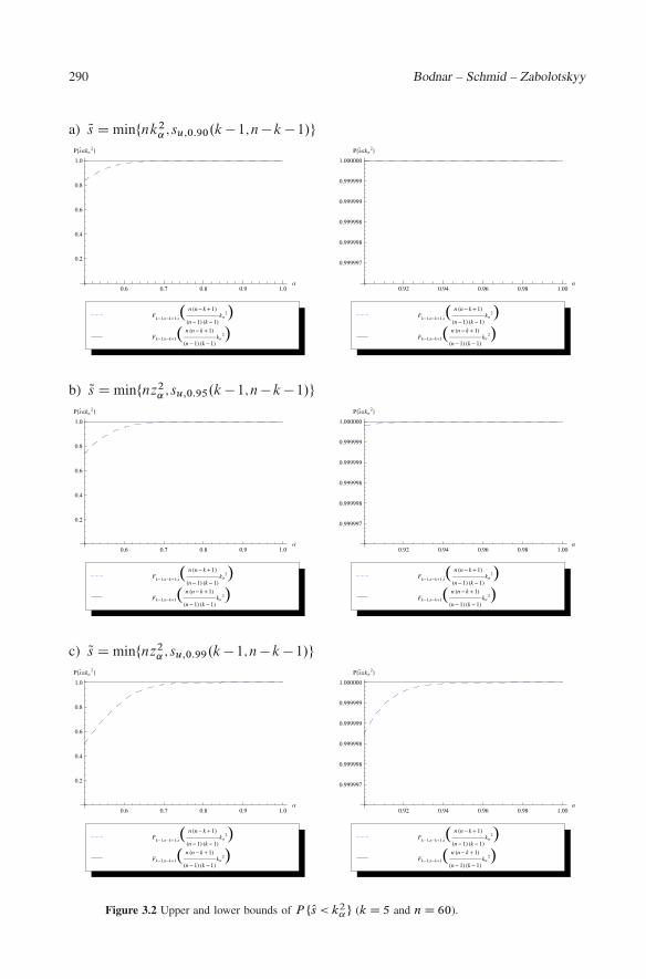
Figure 3.2 Upper and lower bounds of P ¹Os < k2˛º (k D 5 and n D 60).


for ˛ � 0:7 with a high probability. The obtained results are in line with the findings ofAlexander and Baptista (2004) who showed that the existence of the VaR portfolio at theconfidence level ˛ implies the existence of the CVaR portfolio at the same confidencelevel. The extremal behaviour of P.Os < k2

˛/ follows from the fact that k2˛ is always larger

than z2˛ and it tends to infinity much faster than z2

˛.

3.1 1-Parameter case

It is obvious that the minimum value-at-risk optimal portfolio exists only if the inequalitys < z2

˛ holds. From the other side, the estimator of the minimum VaR portfolio istractable iff Os < z2

˛ . Because of these two facts, we study the distributional propertiesof the estimated characteristics of the minimum VaR portfolio under the condition thatOs < z2

˛ . Hence, the distributions of ORVaRjOs < z2˛ , OVVaRjOs < z2

˛ , and OMVaRjOs < z2˛ are derived

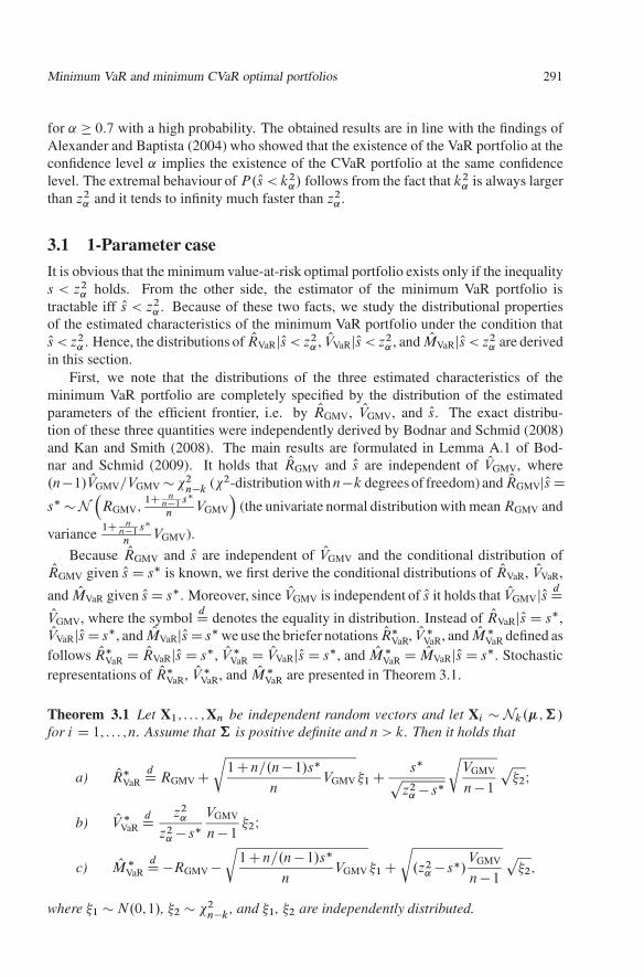
in this section.First, we note that the distributions of the three estimated characteristics of the

minimum VaR portfolio are completely specified by the distribution of the estimatedparameters of the efficient frontier, i.e. by ORGMV, OVGMV, and Os. The exact distribu-tion of these three quantities were independently derived by Bodnar and Schmid (2008)and Kan and Smith (2008). The main results are formulated in Lemma A.1 of Bod-nar and Schmid (2009). It holds that ORGMV and Os are independent of OVGMV, where.n�1/ OVGMV=VGMV � �2

n�k(�2-distribution with n�k degrees of freedom) and ORGMVjOs D

s� � N�RGMV;

1C nn�1

s�

nVGMV

�(the univariate normal distribution with mean RGMV and

variance1C n

n�1s�

nVGMV).

Because ORGMV and Os are independent of OVGMV and the conditional distribution ofORGMV given Os D s� is known, we first derive the conditional distributions of ORVaR, OVVaR,

and OMVaR given Os D s�. Moreover, since OVGMV is independent of Os it holds that OVGMVjOs dDOVGMV, where the symbol

dD denotes the equality in distribution. Instead of ORVaRjOs D s�,OVVaRjOs D s�, and OMVaRjOs D s� we use the briefer notations OR�

VaR, OV �VaR, and OM �

VaR defined asfollows OR�

VaR D ORVaRjOs D s�, OV �VaR D OVVaRjOs D s�, and OM �

VaR D OMVaRjOs D s�. Stochasticrepresentations of OR�


VaR are presented in Theorem 3.1.

Theorem 3.1 Let X1; : : : ;Xn be independent random vectors and let Xi � Nk.�;†/

for i D 1; : : : ;n. Assume that † is positive definite and n > k. Then it holds that

a) OR�VaR

dD RGMV Cr

1 Cn=.n� 1/s�n

VGMV �1 C s�pz2

˛ � s�

rVGMV

n� 1

p�2I

b) OV �VaR

dD z2˛

z2˛ � s�

VGMV

n� 1�2I

c) OM �VaR

dD �RGMV �r

1 Cn=.n� 1/s�n

VGMV �1 Cr

.z2˛ � s�/

VGMV

n� 1

p�2;

where �1 � N.0;1/, �2 � �2n�k

, and �1, �2 are independently distributed.


Proof: The results of Theorem 3.1 follow from (3.1)–(3.3) and the fact that ORGMVjOs Ds� dD RGMV Cp

.1 Cn=.n� 1/s�/=np

VGMV �1 and OVGMVdD .VGMV=.n� 1// �2 (see

Lemma A.1 of Bodnar and Schmid (2009)). �

The results of Theorem 3.1 possess several interesting applications. First, for sim-ulating OR�


VaR it is not necessary to generate n independent k-variatenormally distributed random vectors. It is enough to simulate two random variables �1

and �2 that are independently distributed and have well-known univariate distributionsand then to apply the expressions of Theorem 3.1. Second, Theorem 3.1 is very usefulfor the derivation of the conditional densities of ORVaR, OVVaR, and OMVaR given Os D s�. Let

az.s�/ D s�pz2

˛ � s�

rVGMV

n� 1; bz.s�/ D z2

˛

z2˛ � s�

VGMV

n� 1;

cz.s�/ Dr

.z2˛ � s�/

VGMV

n� 1; Qs� D 1 Cn=.n� 1/s�

nVGMV; (3.9)

It holds that



a) f OR�

VaR.xjs�/ D 1

2.n�k/=2�1az.s�/n�k�..n� k/=2/

exp°

� .x � RGMV/2

2.az.s�/2 C Qs�/

±M.xIn� k;RGMV;

pQs�;az.s�//;

b) f OV �

VaR.xjs�/ D 1

.2bz.s�//.n�k/=2�..n� k/=2/x.n�k/=2�1 exp

°� x

2bz.s�/

±;

c) f OM �

VaR.xjs�/ D 1

2.n�k/=2�1cz.s�/n�k�..n� k/=2/

exp°

� .x CRGMV/2

2.cz.s�/2 C Qs�/

±M.xIn� k;�RGMV;�pQs�;cz.s�//;

where

M.xIm;a;b1;b2/

D 1p2�jb1j

1Z0

tm�1 exp°

� 1

2

�1

b21

C 1

b22

��t � .x � a/

b22

b22 Cb2

1

�2±dt:

The proof of Theorem 3.2 is given in the Appendix.Next, we derive the densities of the estimated characteristics of the minimum VaR

portfolio given that Os < z2˛ . Let

K.v/ D n.n� k C1/

.n� 1/.k � 1/

1

Fk�1;n�kC1Ins. n.n�kC1/.n�1/.k�1/

v/: (3.10)


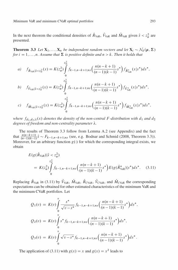
In the next theorem the conditional densities of ORVaR, OVVaR and OMVaR given Os < z2˛ are

presented.



a) f ORVaRjOs<z2˛.x/ D K.z2

˛/

z2Z0

fk�1;n�kC1Ins

� n.n� k C1/

.n� 1/.k � 1/s��f OR�

VaR.xjs�/ds�;

b) f OVVaRjOs<z2˛.x/ D K.z2

˛/

z2Z0

fk�1;n�kC1Ins

� n.n� k C1/

.n� 1/.k � 1/s��f OV �

VaR.xjs�/ds�;

c) f OMVaRjOs<z2˛.x/ D K.z2

˛/

z2Z0

fk�1;n�kC1Ins

� n.n� k C1/

.n� 1/.k � 1/s��f OM �

VaR.xjs�/ds�;

where fd1;d2I�.x/ denotes the density of the non-central F -distribution with d1 and d2

degrees of freedom and non-centrality parameter �.

The results of Theorem 3.3 follow from Lemma A.2 (see Appendix) and the factthat n.n�kC1/

.n�1/.k�1/Os � Fk�1;n�kC1Ins (see, e.g. Bodnar and Schmid (2008, Theorem 3.3)).

Moreover, for an arbitrary function g.�/ for which the corresponding integral exists, weobtain

E.g. ORVaR/jOs < z2˛/

D K.z2˛/

z2Z0

fk�1;n�kC1Ins

� n.n� k C1/

.n� 1/.k � 1/s��E.g. OR�

VaR/js�/ds�: (3.11)

Replacing ORVaR in (3.11) by OVVaR, OMVaR, ORCVaR, OVCVaR, and OMCVaR the correspondingexpectations can be obtained for other estimated characteristics of the minimum VaR andthe minimum CVaR portfolios. Let

Q1.v/ D K.v/

vZ0

s�p

v � s� fk�1;n�kC1Ins

� n.n� k C1/

.n� 1/.k � 1/s��ds�;

Q2.v/ D K.v/

vZ0

s�fk�1;n�kC1Ins

� n.n� k C1/

.n� 1/.k � 1/s��ds�;

Q3.v/ D K.v/

vZ0

pv � s�fk�1;n�kC1Ins

� n.n� k C1/

.n� 1/.k � 1/s��ds� :

The application of (3.11) with g.x/ D x and g.x/ D x2 leads to




a) E. ORVaRjOs < z2˛/ D RGMV C

r2VGMV

n� 1

�. n�kC12

/

�. n�k2

/Q1.z2

˛/;

b) Var. ORVaRjOs < z2˛/ D 1;

c) E. OVVaRjOs < z2˛/ D 1;

d) E. OMVaRjOs < z2˛/ D �RGMV C

r2VGMV

n� 1

�. n�kC12

/

�. n�k2

/Q3.z2

˛/;

e) Var. OMVaRjOs < z2˛/ D

�1

nC 1

n� 1Q2.z2

˛/

�VGMV

C .n� k/

.n� 1/VGMV.z2

˛ � Q2.z2˛// � 2VGMV

n� 1

�. n�kC12

/2

�. n�k2

/2.Q3.z2

˛//2:

The proof of Theorem 3.4 follows from (3.11), Theorem 3.1, and the facts thatE.�1/ D 0, E.�2

1 / D Var.�1/ D 1, E.p

�2/ D p2�. n�kC1

2/=�. n�k

2/, and E.�2/ D n�k.

It is remarkable that Var. ORVaRjOs < z2˛/ D 1 and Var. ORCVaRjOs < z2

˛/ D 1. Thisshows that the corresponding estimators are heavy tailed distributed. Note that it can beproved that E. ORu

VaRjOs < k2˛/ < 1 and E. ORu

CVaRjOs < k2˛/ < 1 for u 2 Œ0;2/. A similar

result does not hold in the case of OVVaR and OVCVaR for which E. OV uVaRjOs < k2

˛/ < 1 andE. OV u

CVaRjOs < k2˛/ < 1 only for u 2 Œ0;1/. Hence, both the estimators OVVaR and OVCVaR

have extremely large tails. From the other side we observe that the expectation and thevariance of OMVaR and OMCVaR do exist. It constitutes a further advantage of the VaR (CVaR)measures and make these measures more attractive than the variance. The estimators ofthe VaR and the CVaR are statistically tractable for the minimum VaR and the minimumCVaR portfolios, while the expectations of the corresponding estimated variances do notexist at all.

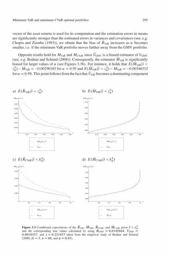
Theorem 3.4 possesses another interesting application. The results can be applied forstudying the conditional bias of the estimators. In Figure 3.3 we present the true valuesof RVaR, MVaR, RCVaR, MCVaR and the corresponding conditional expectations derived inTheorem 3.4. For the calculation we use RGMV D 0:0145664, VGMV D 0:0010337, ands D 0:221457. In the figures, we observe larger deviations in the case of small values of˛ for RVaR and RCVaR. For larger values of ˛, the conditional expectation of the expectedreturn of the minimum VaR portfolio tends to its true value which is almost equal tothe expected return of the global minimum variance portfolio. Such a result is expectedsince the weights of the population minimum VaR portfolio tends to the weights of theglobal minimum variance portfolio and ORGMV is an unbiased estimator of RGMV (cf.,Bodnar and Schmid (2009, Lemma A.1)). On the other hand, for smaller values of ˛

the minimum VaR portfolio deviates from the GMV portfolio although it still lies on theefficient frontier and, hence, it is mean-variance efficient. Because the estimated mean


vector of the asset returns is used for its computation and the estimation errors in meansare significantly stronger than the estimated errors in variances and covariances (see, e.g.Chopra and Ziemba (1993)), we obtain that the bias of ORVaR increases as ˛ becomessmaller, i.e. if the minimum VaR portfolio moves further away from the GMV portfolio.

Opposite results hold for MVaR and MCVaR since OVGMV is a biased estimator of VGMV

(see, e.g. Bodnar and Schmid (2008)). Consequently, the estimator OMVaR is significantlybiased for larger values of ˛ (see Figures 3.3b). For instance, it holds that E. OMVaRjOs <

z2˛/ � MVaR D �0:00290185 for ˛ D 0:95 and E. OMVaRjOs < z2

˛/ � MVaR D �0:00346552

for ˛ D 0:99. This point follows from the fact that OVVaR becomes a dominating component

a) E. ORVaRjOs < z2˛/

0.75 0.80 0.85 0.90 0.95 1.00Α

0.020

0.025

0.030

0.035

0.040

0.045

E�R�

VaR �s��zΑ

2�

RVaR

E�R�

VaR �s��zΑ

2�

b) E. OMVaRjOs < z2˛/

0.75 0.80 0.85 0.90 0.95 1.00Α

0.00

0.02

0.04

0.06

0.08

0.10

E�M�

VaR �s��zΑ

2�

MVaR

E�M�

VaR �s��zΑ

2�

c) E. ORCVaRjOs < k2˛/

0.6 0.7 0.8 0.9 1.0Α

0.020

0.025

0.030

0.035

E�R�

CVaR �s��kΑ

2�

RCVaR

E�R�

CVaR �s��kΑ

2�

d) E. OMCVaRjOs < k2˛/

0.6 0.7 0.8 0.9 1.0Α

0.00

0.02

0.04

0.06

0.08

0.10

E�M�

CVaR �s��kΑ

2�

MCVaR

E�M�

CVaR �s��kΑ

2�

Figure 3.3 Conditional expectations of the ORVaR, OMVaR, ORCVaR, and OMCVaR given Os < z2˛

and the corresponding true values calculated by using RGMV D 0:0145664, VGMV D0:0010337, and s D 0:221457 taken from the empirical study of Bodnar and Schmid(2009) (k D 5, n D 60, and ˛ D 0:95).


in (3.3) for larger values of ˛. Similar results are obtained for the estimated characteristicsof the minimum CVaR portfolio (cf. Figures 3.3c–d). Note that ORCVaR tends much fasterto RCVaR as the estimator ORVaR to RVaR which follows from the fact that k˛ > z˛ .

3.2 2-Parameter caseIn this section we present the conditional distributions of . ORVaR; OVVaR/0 and. ORVaR; OMVaR/0 as well as of . ORCVaR; OVCVaR/0 and . ORCVaR; OMCVaR/0 provided that Os < z2

˛

(Os < k2˛). The results are used to derive the confidence region for the minimum VaR and

the minimum CVaR portfolio as well as the corresponding inference procedures.

3.2.1 Expected return and variance

First, we derive the conditional distribution of . ORVaR; OVVaR/0 given Os D s�, i.e. thedistribution of . OR�

VaR; OV �VaR/0. The results are presented in Theorem 3.5.



f OR�

VaR; OV �

VaR.x1;x2/ D .n� 1/.z2

˛ � s�/

VGMVz2˛

q1Cn=.n�1/s�

nVGMV

fn�k

�.n� 1/x2.z2

˛ � s�/

VGMVz2˛

�

��

0B@ 1q

1Cn=.n�1/s�

nVGMV

�x1 � RGMV � s�p

x2

z˛

�1CA ;

where �.x/ is the density function of the standard normal distribution and fn�k.x/

denotes the density function of the �2-distribution with n� k degrees of freedom.

The proof of Theorem 3.5 is given in the Appendix.The distribution of . ORVaR; OVVaR/0jOs < z2

˛ and of . ORCVaR; OVCVaR/0jOs < k2˛ is obtained by

applying an extension of Lemma A.2. It holds that

f ORVaR; OVVaRjOs<z2˛.x1;x2/

D K.z2˛/

z2Z0

fk�1;n�kC1Ins

�n.n� k C1/

.n� 1/.k � 1/s��

f OR�

VaR; OV �

VaR.x1;x2js�/ds� :

For the GMV portfolio it holds that ORGMV and OVGMV are independently distributed.However, this nice property does not hold in the case of the minimum VaR portfolio orin the case of the minimum CVaR portfolio.

From Theorem 3.1 and the extension of (3.11) we obtain

Cov. ORVaR; OVVaRjOs < z2˛/ D 1 and Cov. ORCVaR; OVCVaRjOs < z2

˛/ D 1: (3.12)


Since both the covariances and the variances are infinite, we are not able to calculatethe Pearson correlation coefficient between ORVaR and OVVaR. Instead of this quantity wecompute the average correlation coefficient defined by

Corr. ORVaR; OVVaRjOs < z2˛/

D K.z2˛/

z2Z0

fk�1;n�kC1Ins

�n.n� k C1/

.n� 1/.k � 1/s��

Corr. ORVaR; OVVaRjOs D s�/ds�

D K.z2˛/p

n� k

�. n�kC12

/

�. n�k2

/(3.13)

�z2Z0

s�fk�1;n�kC1Ins. n.n�kC1/.n�1/.k�1/

s�/vuut.z2˛ � s�/. n�1

nC s�/ C

.n� k/ � 2

��. n�kC1

2/

�. n�k2

/

�2!

.s�/2

ds� :

In the same way Corr. ORCVaR; OVCVaRjOs < k2˛/ is defined. We note that the average cor-

relation coefficient is non-negative because all the quantities in (3.13) are non-negative.Moreover, the definition of Corr.�; �/ ensures that it lies in the interval Œ�1;1� and, conse-quently, it can be used for describing the dependence between two estimators. Further-more, we note that both expressions of the average correlation coefficient between ORVaR

and OVVaR as well as between ORCVaR and OVCVaR show that they depend on � and † onlyover the quantity s. Using s D 0:221457 we plot the quantities Corr. ORVaR; OVVaRjOs < z2

˛/

and Corr. ORCVaR; OVCVaRjOs < k2˛/ as a function of ˛ for several values of the slope parameter

in Figures 3.4a and 3.4b as well as a function of s for ˛ 2 ¹0:9;0:95;0:99º in Figures3.4c and 3.4d. We observe that a moderate amount of linear dependence is present inthe estimators ORVaR and OVVaR, while a small amount of linear dependence is observedbetween ORCVaR and OVCVaR. For the minimum CVaR portfolio the average correlationcoefficient is smaller than in the case of the minimum VaR portfolio. From the otherside, both average correlation coefficients are positive for all values of ˛. The point isin line with the financial literature. It is impossible to get a higher expected return ofthe portfolio without increasing the portfolio risk. The highest dependence is present forsmaller values of ˛ in the case of the minimum VaR portfolio. Finally, for the values of˛, that are close to 1, the average correlation coefficient tends to zero since the minimumVaR portfolio tends to the GMV portfolio as ˛ ! 1 and the estimated expected returnand the estimated variance of the GMV portfolio are independent (see, e.g., Bodnar andSchmid (2009, Lemma A.1)). In Figures 3.4c and 3.4d we observe that the consideredaverage correlation coefficients are increasing functions of s. Moreover, for s D 0 a verysmall amount of linear dependence is present in both the expressions which follows fromthe fact that in the limit case of s D 0 both the minimum VaR and the minimum CVaRportfolios coincide with the GMV portfolio and its estimated characteristics are indepen-dently distributed. From the other side, in the case of common values of the parameters, which, usually, are observed for real data, the average correlation is above 20% for theminimum VaR portfolio and above 10% for the minimum CVaR portfolio.


a) Corr. ORVaR; OVVaRjOs < z2˛/

0.75 0.80 0.85 0.90 0.95 1.00Α

0.1

0.2

0.3

0.4

0.5

0.6

0.7

Corr�R�

VaR,V�

VaR �s��zΑ

2�

2s

s�2

s0.221457

b) Corr. ORCVaR; OVCVaRjOs < k2˛/

0.75 0.80 0.85 0.90 0.95 1.00Α

0.05

0.10

0.15

0.20

0.25

0.30

Corr�R�

CVaR,V�

CVaR �s��kΑ

2�

2s

s�2

s0.221457

c) Corr. ORVaR; OVVaRjOs < z2˛/

0.2 0.4 0.6 0.8 1.0 1.2s

0.1

0.2

0.3

0.4

0.5

0.6

Corr�R�

VaR,V�

VaR �s��zΑ

2�

Α0.99

Α0.95

Α0.9

d) Corr. ORCVaR; OVCVaRjOs < k2˛/

0.2 0.4 0.6 0.8 1.0 1.2s

0.05

0.10

0.15

0.20

0.25

0.30

0.35

Corr�R�

CVaR,V�

CVaR �s��kΑ

2�

Α0.99

Α0.95

Α0.9

Figure 3.4 The average correlation coefficients Corr. ORVaR; OVVaRjOs < z2˛/ and

Corr. ORCVaR; OVCVaRjOs < z2˛/ as a function of s and ˛ (k D 5 and n D 60).

Next, we present a joint confidence region for .RVaR;VVaR/0. Let 1 � ˇ D .1 � Q/3,that is, Q D 1 � 3

p1 � ˇ. By sl and su we denote the lower and the upper borders of the

confidence interval for the slope parameter s which are calculated recursively (see, e.g.Bodnar and Schmid (2009, Section 7.2)). Let

g1.s;v/ D ORGMV C

s � pv � sz

1� Q=2

r1

nC Os

n� 1

!rV

v; (3.14)

g2.s;v/ D ORGMV C

s Cpv � sz

1� Q=2

r1

nC Os

n� 1

!rV

v; (3.15)

rl.v/ D v

0@1 � 1

V

.n� 1/ OVGMV

�2

n�kI Q=2

1A ; (3.16)


ru.v/ D v

0@1 � 1

V

.n� 1/ OVGMV

�2

n�kI1� Q=2

1A ; (3.17)

s�u.v/ D v �

z2

1� Q=2

4

�1

nC Os

n� 1

�: (3.18)

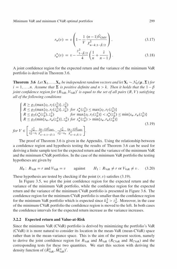
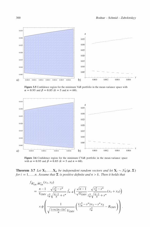
A joint confidence region for the expected return and the variance of the minimum VaRportfolio is derived in Theorem 3.6.

Theorem 3.6 Let X1; : : : ;Xn be independent random vectors and let Xi � Nk.�;†/ fori D 1; : : : ;n. Assume that † is positive definite and n > k. Then it holds that the 1 � ˇ

joint confidence region for .RVaR;VVaR/0 is equal to the set of all pairs .R;V / satisfyingall of the following conditions8

<ˆ:

R � g1.max¹sl ; rl.z2˛/º;z2

˛/


˛/ for s�u.z2

˛/ � max¹sl ; rl .z2˛/º

R � g2.s�u.z2

˛/;z2˛/ for max¹sl ; rl.z

2˛/º < s�

u.z2˛/ � min¹su; ru.z2

˛/ºR � g2.min¹su; ru.z2

˛/º;z2˛/ for s�

u.z2˛/ > min¹su; ru.z2

˛/º(3.19)

for V 2�

z2˛

z2˛�sl

.n�1/ OVGMV

�2

n�kI1� Q=2

;z2

˛

z2˛�su

.n�1/ OVGMV

�2

n�kI Q=2

�.

The proof of Theorem 3.6 is given in the Appendix. Using the relationship betweena confidence region and hypothesis testing the results of Theorem 3.6 can be used forderiving a finite sample test for the expected return and the variance of the minimum VaRand the minimum CVaR portfolios. In the case of the minimum VaR portfolio the testinghypotheses are given by

H0 W RVaR D r and VVaR D v against H1 W RVaR ¤ r or VVaR ¤ v : (3.20)

These hypothesis are tested by checking if the point .r;v/ satisfies (3.19).In Figure 3.5, we plot the joint confidence region for the expected return and the

variance of the minimum VaR portfolio, while the confidence region for the expectedreturn and the variance of the minimum CVaR portfolio is presented in Figure 3.6. Theconfidence region for the minimum CVaR portfolio is smaller than the confidence regionfor the minimum VaR portfolio which is expected since k2

˛ > z2˛ . Moreover, in the case

of the minimum CVaR portfolio the confidence region is moved to the left. In both casesthe confidence intervals for the expected return increase as the variance increases.

3.2.2 Expected return and Value-at-Risk

Since the minimum VaR (CVaR) portfolio is derived by minimizing the portfolio’s VaR(CVaR) it is more natural to consider its location in the mean-VaR (mean-CVaR) spacerather than in the mean-variance space. This is the aim of the present section, namelyto derive the joint confidence region for RVaR and MVaR (RCVaR and MCVaR) and thecorresponding tests for these two quantities. We start this section with deriving thedensity function of . OR�

VaR; OM �VaR/0.


a) 0.0010 0.0011 0.0012 0.0013 0.0014 0.0015 0.0016

0.005

0.010

0.015

0.020

0.025

0.030

0.035

b) 0.0010 0.0012 0.0014 0.0016V

0.005

0.010

0.015

0.020

0.025

0.030

0.035

R

Figure 3.5 Confidence region for the minimum VaR portfolio in the mean-variance space with˛ D 0:95 and ˇ D 0:85 (k D 5 and n D 60).

a) 0.0010 0.0012 0.0014 0.0016

0.005

0.010

0.015

0.020

0.025

0.030

0.035

b) 0.0010 0.0012 0.0014 0.0016V

0.005

0.010

0.015

0.020

0.025

0.030

0.035R

Figure 3.6 Confidence region for the minimum CVaR portfolio in the mean-variance spacewith ˛ D 0:95 and ˇ D 0:85 (k D 5 and n D 60).



f OR�

VaR; OM �

VaR.x1;x2/

D n� 1

VGMV

pz2

˛ � s�

z2˛

qn�1

nC s�

Qfn�k

�pn� 1pVGMV

pz2

˛ � s�

z2˛

qn�1

nC s�

.x1 Cx2/�

� �

0B@ 1q

1Cn=.n�1/s�

nVGMV

�.z2

˛ � s�/x1 � s�x2

z2˛

� RGMV

�1CA :


where �.x/ is the density function of the standard normal distribution, and Qfn�k.x/

denotes the density function of the �-distribution with n� k degrees of freedom.

The proof of Theorem 3.7 is given in the Appendix.The application of the extension of Lemma A.2 leads to the following density of

. ORVaR; OMVaR/0 given Os < z2˛

f ORVaR; OMVaRjOs<z2˛.x1;x2/

D K.z2˛/

z2Z0

fk�1;n�kC1Ins

�n.n� k C1/

.n� 1/.k � 1/s��

f OR�

VaR; OM �

VaR.x1;x2js�/ds� :

Next, we study the dependence properties of the estimators. The application ofTheorem 3.1 and the extension of (3.11) leads to the expressions of the covariances. Forthe minimum VaR portfolio it is given by

Cov. ORVaR; OMVaRjOs < z2˛/ D �VGMV

�1

nC 1

n� 1Q2.z2

˛/

�C n� k

n� 1VGMVQ2.z2

˛/

� 2VGMV

n� 1

�. n�kC1

2/

�. n�k2

/

!2

Q1.z2˛/Q3.z2

˛/: (3.21)

Opposite to the case of the expected return and the variance, the covariance betweenthe expected return and the value-at-risk is finite. However, because the covariance isnot normalized it cannot be used to investigate how large is the dependence between tworandom variables. Its standardized quantity, namely the correlation, should be appliedfor such purposes. Unfortunately, the variances of ORVaR is infinite (see Theorem 3.4) andconsequently, the Pearson correlation coefficients between ORVaR and OMVaR could not becalculated. From the other side the average correlation coefficient defined in Section 3.2.1is finite and it is given by

Corr. ORVaR; OMVaRjOs < z2˛/ (3.22)

D K.z2˛/

z2Z0

fk�1;n�kC1Ins

�n.n�k C1/

.n�1/.k �1/s��

Corr. ORVaR; OMVaRjs�/ds�;

Corr. ORVaR; OMVaRjOs D s�/ (3.23)

D

�. n�1

n C s�/C s�

n�k �2

��. n�kC1

2 /

�. n�k2 /

�2!!

vuut.z2˛ � s�/. n�1

n C s�/C

n�k �2

��. n�kC1

2 /

�. n�k2 /

�2!

.s�/2

�p

z2˛ � s�vuutn�1

n C s� C

n�k �2

��. n�kC1

2/

�. n�k2

/

�2!

.z2˛ � s�/

:


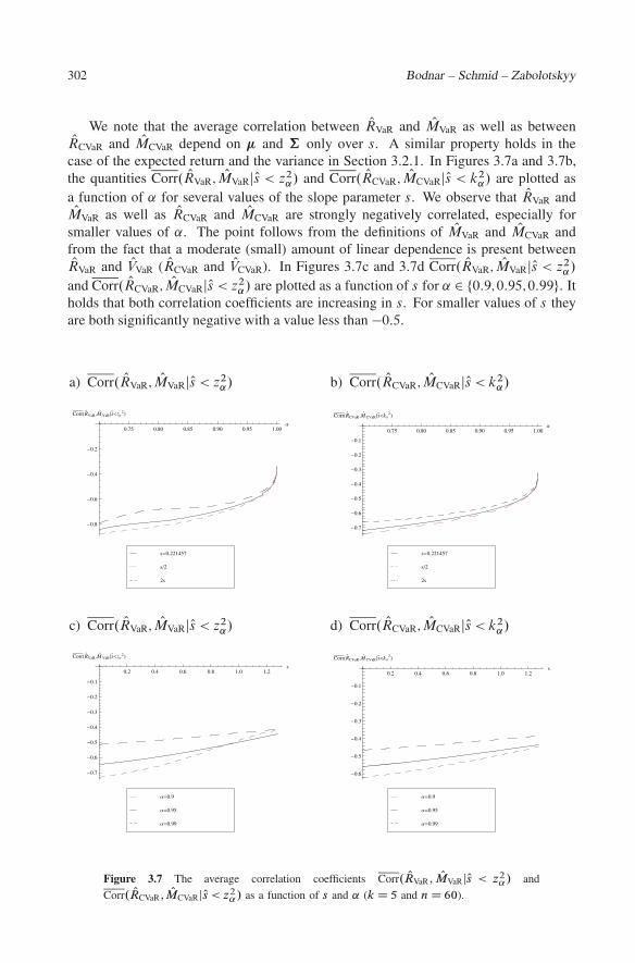
We note that the average correlation between ORVaR and OMVaR as well as betweenORCVaR and OMCVaR depend on � and † only over s. A similar property holds in the

case of the expected return and the variance in Section 3.2.1. In Figures 3.7a and 3.7b,the quantities Corr. ORVaR; OMVaRjOs < z2

˛/ and Corr. ORCVaR; OMCVaRjOs < k2˛/ are plotted as

a function of ˛ for several values of the slope parameter s. We observe that ORVaR andOMVaR as well as ORCVaR and OMCVaR are strongly negatively correlated, especially for

smaller values of ˛. The point follows from the definitions of OMVaR and OMCVaR andfrom the fact that a moderate (small) amount of linear dependence is present betweenORVaR and OVVaR ( ORCVaR and OVCVaR). In Figures 3.7c and 3.7d Corr. ORVaR; OMVaRjOs < z2

˛/

and Corr. ORCVaR; OMCVaRjOs < z2˛/ are plotted as a function of s for ˛ 2 ¹0:9;0:95;0:99º. It

holds that both correlation coefficients are increasing in s. For smaller values of s theyare both significantly negative with a value less than �0:5.

a) Corr. ORVaR; OMVaRjOs < z2˛/

0.75 0.80 0.85 0.90 0.95 1.00Α

�0.8

�0.6

�0.4

�0.2

Corr�R�

VaR,M�

VaR �s��zΑ

2�

2s

s�2

s0.221457

b) Corr. ORCVaR; OMCVaRjOs < k2˛/

0.75 0.80 0.85 0.90 0.95 1.00Α

�0.7

�0.6

�0.5

�0.4

�0.3

�0.2

�0.1

Corr�R�

CVaR,M�

CVaR �s��kΑ

2�

2s

s�2

s0.221457

c) Corr. ORVaR; OMVaRjOs < z2˛/

0.2 0.4 0.6 0.8 1.0 1.2s

�0.7

�0.6

�0.5

�0.4

�0.3

�0.2

�0.1

Corr�R�

VaR,M�

VaR �s��zΑ

2�

Α0.99

Α0.95

Α0.9

d) Corr. ORCVaR; OMCVaRjOs < k2˛/

0.2 0.4 0.6 0.8 1.0 1.2s

�0.6

�0.5

�0.4

�0.3

�0.2

�0.1

Corr�R�

CVaR,M�

CVaR �s��kΑ

2�

Α0.99

Α0.95

Α0.9

Figure 3.7 The average correlation coefficients Corr. ORVaR; OMVaRjOs < z2˛/ and

Corr. ORCVaR; OMCVaRjOs < z2˛/ as a function of s and ˛ (k D 5 and n D 60).


Next, we present a joint confidence region for .RVaR;MVaR/0. Let

Qg1.s;v/ D ORGMV C

s � pv � sz

1� Q=2

r1

nC Os

n� 1

!R CM

v; (3.24)

Qg2.s;v/ D ORGMV C

s Cpv � sz

1� Q=2

r1

nC Os

n� 1

!R CM

v; (3.25)

Qrl.v/ D v

0@1 � v

.R CM /2

.n� 1/ OVGMV

�2

n�kI Q=2

1A ; (3.26)

Qru.v/ D v

0@1 � v

.R CM /2

.n� 1/ OVGMV

�2

n�kI1� Q=2

1A : (3.27)

Theorem 3.8 Let X1; : : : ;Xn be independent random vectors and let Xi � Nk.�;†/ fori D 1; : : : ;n. Assume that † is positive definite and n > k. Then it holds that the 1 � ˇ

joint confidence region for .RVaR;MVaR/0 is equal to the set of all pairs .R;M / satisfyingall of the following conditions

8<ˆ:

R � Qg1.max¹sl ; Qrl.z2˛/º;z2

˛/

R � Qg2.max¹sl ; Qrl.z2˛/º;z2

˛/ for s�u.z2

˛/ � max¹sl ; Qrl .z2˛/º

R � Qg2.s�u.z2

˛/;z2˛/ for max¹sl ; Qrl.z

2˛/º < s�

u.z2˛/ � min¹su; Qru.z2

˛/ºR � Qg2.min¹su; Qru.z2


u.z2˛/ > min¹su; Qru.z2

˛/º(3.28)

forr

.n�1/ OVGMV

�2n�kI1�ˇ=2

z2˛p

z2˛�max¹sl ;Qrl .z2

˛/º � R CM �r

.n�1/ OVGMV

�2n�kIˇ=2

z2˛p

z2˛�min¹su;Qru.z2

˛/º .

The proof of Theorem 3.8 is given in the Appendix.Following the discussion at the end of Section 3.2.1 we suggest a finite sample test

for the expected return and the VaR (CVaR) of the minimum VaR (CVaR) portfolio. Inthe case of the minimum VaR portfolio the testing hypotheses are given by

H0 W RVaR D r and MVaR D m against H1 W RVaR ¤ r or MVaR ¤ m: (3.29)

These hypothesis are tested by checking if the point .r;m/ satisfies (3.28). A similartesting procedure is obtained in the case of the minimum CVaR portfolio.

4 SummaryIn the pioneering work of Markowitz (1952) an optimal portfolio is obtained by mini-mizing the portfolio variance for a given value of the portfolio return. Although in themeantime many other approaches for constructing an optimal portfolio have been intro-duced, the mean-variance analysis of Markowitz (1952) is still the most popular methodin practice. For a long time one of the crucial assumptions for the derivation of the optimalportfolio weights was that the parameters of the underlying return process are known.


Another crucial assumption of the Markowitz theory for optimal portfolio selection is theapplication of the variance as a risk proxy.

In the present paper, we consider the estimators for the characteristics of the minimumVaR and the CVaR portfolios and present their small sample densities. These expressionsare used for studying the distributional properties of the estimated characteristics. Weprove that the expectation does not exist for the estimated variance, while the secondmoment does not exist for the estimated expected return. We also give the expressionsfor the joint densities and derive the corresponding dependence measures between theestimators for the expected return and the variance as well as between the estimated ex-pected return and the estimated VaR (CVaR). Moreover, we present an exact finite sampleconfidence region for the minimum VaR portfolio and the minimum CVaR portfolio inthe mean-variance space as well as in the mean-VaR (mean-CVaR) space. The obtainedresults are illustrated in an empirical study throughout the paper by using the estimatorsfor the parameters of the efficient frontier given in Bodnar and Schmid (2009).

A AppendixA.1 Derivation of wVaR and wCVaR

First, we derive the expression of the minimum VaR portfolio weights in terms of wGMV,RGMV, VGMV, and s. Let A D 10†�1�, B D �0†�1�, C D 10†�11, and D D BC �A2 DsC with s D B � A2=C . Let g D 1=D.B†�11 � A†�1�/ and h D 1=D.C †�1� �A†�11/. The weights of the minimum VaR portfolio are given by (see Alexander andBaptista (2004, Proposition 1))

wVaR D g C hV˛ D 1

D.B � AV˛/†�11 C 1

D.C V˛ � A/†�1� (A.1)

with

V˛ D A

CCs

s2

z2˛ � s

1

CD RGMV C s

pVGMVp

z2˛ � s

:

With some mathematics from (A.1) we get

wVaR D wGMV C�

B

D� A

DV˛ � 1

C

�†�11 C

�C

DV˛ � A

D

�†�1�

D wGMV C

s CA2=C

D� A2

CD� 1

C� A

D

spCp

z2˛ � s

!†�11

C

CA=C

D� A

DC C

D

spCp

z2˛ � s

!†�1�

D wGMV � RGMV

pVGMVpz2

˛ � s†�11 C

pVGMVpz2

˛ � s†�1�

D wGMV Cp

VGMVpz2

˛ � sR� :


Similarly, the weights of the minimum CVaR portfolio are expressed as (cf.,Alexanderand Baptista (2004, p. 1263))

wCVaR D g C hL˛ D 1

D.B � AL˛/†�11 C 1

D.CL˛ � A/†�1�

D wGMV Cp

VGMVpk2

˛ � sR�

with

L˛ D A

CCs

s2

k2˛ � s

1

CD RGMV C s

pVGMVp

k2˛ � s

;

where k˛ is defined in (2.9). The formulas for the expected return, the variance, and the(conditional) value-at-risk of both the optimal portfolios are obtained by straightforwardcalculations from the expressions of the weights.

A.2 Proofs of Lemmas and TheoremsLemma A.1 Let 1 and 2 be independently distributed with 1 � N .a;b1/ and 2 � �2

m.Then for a;b1 2 R, b1 > 0 and b2 2 RC the density of D aCb11 Cb2

p2 is given by

f� .x/ D 1

2m=2�1bm2 �.m=2/

exp°

� .x � a/2

2.b22 Cb2

1/

±M.xIm;a;b1;b2/;

where

M.xIm;a;b1;b2/

D 1p2�jb1j

1Z0

tm�1 exp°

� 1

2

�1

b21

C 1

b22

��t � .x � a/

b22

b22 Cb2

1

�2±dt:

Proof: Let Q1 D a C b11 � N .a;b21/. The density of Q1 we denote by fQ�1

.x/. Let

fb2

p�2

.x/ be the density of b2

p2. From the fact that 2 � �2-distributed with m

degrees of freedom we get

fb2

p�2

.x/ D f�2.x2=b2

2/2x

b22

D 1

2m=2�1bm2 �.m=2/

xm�1 exp°

� x2

2b22

±:

Because Q1 and 2 are independently distributed the density of is obtained by usingthe convolution product of two densities fQ�1

.�/ and fb2

p�2

.�/. It is given by

f� .x/ D1Z0

fQ�1.x � t/fb2

p�2

.t/dt D1Z0

1p2�jb1j exp

°� 1

2b21

.x � t � a/2±

� 1

2m=2�1bm2 �.m=2/

tm�1 exp°

� t2

2b22

±dt

D1Z0

1p2�jb1j2m=2�1bm

2 �.m=2/tm�1 exp

°� 1

2b21

.x � t � a/2 � t2

2b22

±dt:


The power of the exponent in the previous integral can be rewritten in the following form

� 1

2b21

.x � t � a/2 � t2

2b22

D � 1

2b21

�t2 C .x � a/2 � 2t.x � a/

� t2

2b22

D � 1

2b21

�t2 C .x � a/2 � 2t.x � a/ C t2b2

1

b22

�

D �1

2

�1

b21

C 1

b22

��t � .x � a/

b22

b22 Cb2

1

�2 � .x � a/2

2.b21 Cb2

2/:

Substituting the last identity in the expression of f� .x/ we obtain the statement of thelemma. �

Proof of Theorem 3.2:

a) The results of Theorem 3.1a follow from Lemma A.1 with a D RGMV, b1 Dq1Cn=.n�1/s�

nVGMV, b2 D s�p

z2˛�s�

VGMVn�1

, and m D n� k.

b) The result follows from Theorem 3.1b and the identity �2 � �2n�k

. It holds that

f OV �

VaR.x/ D 1

bz.Qs�/f�2

.x=bz.Qs�//

D 1

.2bz.Qs�//.n�k/=2�..n� k/=2/x.n�k/=2�1 exp

°� x

2bz.Qs�/

±:

c) The results of Theorem 3.1c follow from Lemma A.1 with a D �RGMV, b1 D�q

1Cn=.n�1/s�

nVGMV, b2 D

q.z2

˛ � s�/ VGMVn�1

, and m D n� k. �

In order to proof the Theorem 3.3 we need the following lemma.

Lemma A.2 Assume that the 2-dimensional random vector .X;Y /0 is absolutely con-tinuous. Let fY .�/ denote the density of Y and FY .�/ the distribution function. LetfX jY Dy.�jt/ be the density of X given Y D y. Then

fX jY �y.xjy/ D 1

FY .y/

yZ�1

fX jY Dt .xjt/fY .t/dt

is a density of X given Y � y.

Proof: Let FX jY �y.xjy/ be the distribution function of X given Y � y. Then it holdsthat

FX jY �y.xjy/ D P.¹X � xº \ ¹Y � yº/P ¹Y � yº D 1

FY .y/

xZ�1

yZ�1

f .; t/ddt;

where f .; t/ is the joint density of X and Y .


Using the fact that f .; t/ D fX jY Dt. jt/fY .t/ we obtain

FX jY �y.xjy/ D 1

FY .y/

xZ�1

� yZ�1

fX jY Dt. jt/fY .t/dt�d

and, thus,

fX jY �y.xjy/ D @FX jY �y.xjy/

@xD 1

FY .y/

yZ�1

fX jY Dt.xjt/fY .t/dt:

is a density of X given Y � y. �

Proof of Theorem 3.5: From Theorem 3.1 it follows that² OR�

VaR D RGMV CpQs� �1 Caz.s�/p

�2

OV �VaR D bz.s�/�2

;

where az.s�/, bz.s�/, and Qs� are defined in (3.9); �1 � N.0;1/, �2 � �2n�k

, and �1, �2

are independently distributed.Solving this system of equations with respect to OR�

VaR and OV �VaR, we obtain

8<:

�2 D 1bz.s�/

OV �VaR

�1 D 1pQs�. OR�

VaR � RGMV � az.s�/

rOV �

VaRbz.s�/

:

Then the Jacobian of the transformation from . OR�VaR; OV �

VaR/ to .�1;�2/ is equal to

ˇˇJ

.�1;�2/

. OR�VaR; OM �

VaR/

!ˇˇ Dˇˇˇ0@

@�1

@ OR�

VaR

@�1

@ OV �

VaR@�2

@ OR�

VaR

@�2

@ OV �

VaR

1Aˇˇˇ

Dˇˇˇ0@ 1pQs�

� az.s�/

2

qOV �

VaRbz.s�/Qs�

0 1bz.s�/

1AˇˇˇD 1

bz.s�/pQs� :

Hence, the joint density of OR�VaR and OV �

VaR is given by

f OR�

VaR; OV �

VaR.x1;x2/ D 1

bz.s�/pQs� fn�k

�x2

bz.s�/

�

� �

�1pQs�

�x1 � RGMV � az.s�/

rx2

bz.s�/

��:

The result of Theorem 3.5 follows. �


Proof of Theorem 3.6: From the definition of RVaR and VVaR we get

VVaR D z2˛

z2˛ � s

VGMV ;

RVaR D RGMV C spz2

˛ � s

pVGMV D RGMV C s

z˛

pVVaR :

Following Bodnar and Schmid (2009) the joint confidence region for the three pa-rameters of the efficient frontier, i.e. for .RGMV;VGMV; s/0, is expressed as

ORGMV � z1� Q=2

r1

nC Os

n� 1

pVGMV � RGMV

� ORGMV C z1� Q=2

r1

nC Os

n� 1

pVGMV

.n� 1/ OVGMV

�2

n�kI1� Q=2

� VGMV � .n� 1/ OVGMV

�2

n�kI Q=2

sl � s � su ;

where sl and su are calculated recursively (see, e.g. Bodnar and Schmid (2009, Sec-tion 7.2)). Rewriting the first two equations with respect to RVaR and VVaR we obtain

ORGMV C

s �q

z2˛ � sz

1� Q=2

r1

nC Os

n� 1

!pVVaR

z˛

� RVaR

� ORGMV C

s Cq

z2˛ � sz

1� Q=2

r1

nC Os

n� 1

!pVVaR

z˛

; (A.2)

z2˛

z2˛ � s

.n� 1/ OVGMV

�2

n�kI1� Q=2

� VVaR � z2˛

z2˛ � s

.n� 1/ OVGMV

�2

n�kI Q=2

; (A.3)

sl � s � su : (A.4)

The expressions (A.2) and (A.3) define a joint confidence region for RVaR and VVaR

for a given s taken from (A.4). In order to eliminate the dependence on s we calculatethe union of the regions (A.2)–(A.3) over s 2 Œsl ; su�. First, for a given value of VVaR, thepossible values of s are determined from (A.3), i.e.,

z2˛

VVaR

.n� 1/ OVGMV

�2

n�kI1� Q=2

� z2˛ � s � z2

˛

VVaR

.n� 1/ OVGMV

�2

n�kI Q=2

Ý

z2˛

0@1 � 1

VVaR

.n� 1/ OVGMV

�2

n�kI Q=2

1A� s � z2

˛

0@1 � 1

VVaR

.n� 1/ OVGMV

�2

n�kI1� Q=2

1A: (A.5)

Taking into account the equations (A.4) and (A.5) as well as the definitions of rl.v/

and ru.v/ (see (3.16) and (3.17)), we define for a fixed value of VVaR the set of possiblevalues of s expressed as

�VaR D ¹s 2 Rjmax¹sl ; rl .z2˛/º � s � min¹su; ru.z2

˛/ºº :


Recalling the definition of the functions g1.s;v/ and g2.s;v/ given in (3.14) and (3.15)correspondingly, we derive the lower border of the confidence region by minimizingg1.s;z2

˛/ over s 2 �VaR, i.e. g1.s;z2˛/ �!

s2�VaR

min. The first derivative is equal to

g01.s;z2

˛/ Dp

VVaR

z˛

0B@1 C

z1� Q=2

q1n

C Osn�1

2p

z2˛ � s

1CA> 0:

Since the first derivative of g1.s;z2˛/ is always positive, the minimum is reached at the

lower border of �VaR. Then the lower border of the confidence region is given by

R � g1.max¹sl ; rl .z2˛/º;z2

˛/ (A.6)

for VVaR 2h

z2˛

z2˛�sl

.n�1/ OVGMV

�2

n�kI1� Q=2

;z2

˛

z2˛�su

.n�1/ OVGMV

�2

n�kI Q=2

i.

Next, we calculate the upper border which is obtained by maximizing g2.s;z2˛/ over

s 2 �VaR, i.e. by solving g2.s;z2˛/ �!

s2�VaR

max. Setting the first derivative of g2.s;z2˛/

equal to zero, we get

g02.s;z2

˛/ Dp

VVaR

z˛

0B@1 �

z1� Q=2

q1n

C Osn�1

2p

z2˛ � s

1CAD 0

Solving the last equality with respect to s yields

s�u.z2

˛/ D z2˛ �

z2

1� Q=2

4

�1

nC Os

n� 1

�(A.7)

Since the second derivative is always negative, i.e.

g002.s;z2

˛/ D � z1� Q=2

q1n

C Osn�1

4.z2˛�s/3=2

pVVaRz˛

< 0;

it holds that that g2.s;z2˛/ reaches its maximum at the point s�

u.z2˛/. Taking into account

that s 2 �VaR, we obtained the following upper border for the confidence region

8<:


˛/ for s�u.z2

˛/ � max¹sl ; rl .z2˛/º

R � g2.s�u.z2

˛/;z2˛/ for max¹sl ; rl.z

2˛/º < s�

u.z2˛/ � min¹su; ru.z2

˛/ºR � g2.min¹su; ru.z2


u.z2˛/ > min¹su; ru.z2

˛/º(A.8)

for VVaR 2h

z2˛

z2˛�sl

.n�1/ OVGMV

�2

n�kI1� Q=2

;z2

˛

z2˛�su

.n�1/ OVGMV

�2

n�kI Q=2

i. Putting (A.3), (A.6), and (A.8), we proof

the result of the theorem. �


Proof of Theorem 3.7: The application of Theorem 3.1 leads to

. OR�VaR; OM �

VaR/0 dD a C A.�1;p

�2/0

where a D .RGMV;�RGMV/0,

A D� p

s� az.s�/

�ps� cz.s�/

�;

where az.s�/, cz.s�/, and Qs� are defined in (3.9); �1 � N.0;1/, �2 � �2n�k

, and �1, �2 areindependently distributed.

Let

Qfn�k.x/ D 1

2.n�k/=2�1�. n�k2

/xn�k�1 exp

°� x2

2

±

denote the density function ofp

�2. Then we obtain

f OR�

VaR; OM �

VaR.x1;x2/ D 1

detA�.¹A�1..x1;x2/0 � a/º1/ Qfn�k.¹A�1..x1;x2/0 � a/º2/;

where ¹A�1..x1;x2/0 � a/ºi is the i -th element of the vector A�1..x1;x2/0 � a/. Thestatement of Theorem 3.7 is proved. �

Proof of Theorem 3.8: From (2.5) and (2.7) we obtain

´VGMV D z2

˛�s

z4˛

.RVaR CMVaR/2

RGMV D RVaR � s

z2˛

.RVaR CMVaR/

The substitution of this quantities in the joint confidence interval for the three param-eters of the efficient frontier (A.2) leads to

ORGMV � z1�ˇ=2

r1

nC Os

n� 1

pz2

˛ � s

z2˛

.RVaR CMVaR/

� RVaR � s

z2˛

.RVaR CMVaR/

� ORGMV C z1�ˇ=2

r1

nC Os

n� 1

pz2

˛ � s

z2˛

.RVaR CMVaR/

.n� 1/ OVGMV

�2n�kI1�ˇ=2

� z2˛ � s

z4˛

.RVaR CMVaR/2 � .n� 1/ OVGMV

�2n�kIˇ=2

sl � s � su :


Rewriting the first two inequalities yields

ORGMV C

s �q

z2˛ � sz1�ˇ=2

r1

nC Os

n� 1

!RVaR CMVaR

z2˛

� RVaR

� ORGMV C

s �q

z2˛ � sz1�ˇ=2

r1

nC Os

n� 1

!RVaR CMVaR

z2˛

(A.9)

vuut .n� 1/ OVGMV

�2n�kI1�ˇ=2

z2˛p

z2˛ � s

� RVaR CMVaR �vuut .n� 1/ OVGMV

�2n�kIˇ=2

z2˛p

z2˛ � s

(A.10)

sl � s � su : (A.11)

The inequalities (A.9)–(A.10) have the same structure as the inequalities (A.2)–(A.3)with RVaR CMVaR to be replaced instead of VVaR. The rest of the proof follows from theproof of Theorem 3.6 by replacing the quantities �VaR, g1.s;z2

˛/ and g2.s;z2˛/ by

Q�VaR D ¹s 2 Rjmax¹sl I Qrl.z2˛/º � s � min¹suI Qru.z2

˛/ºº ;

Qg1.s;z2˛/ D ORGMV C

s �

qz2

˛ � sz1� Q=2

r1

nC Os

n� 1

!RVaR CMVaR

z2˛

;

Qg2.s;z2˛/ D ORGMV C

s C

qz2

˛ � sz1� Q=2

r1

nC Os

n� 1

!RVaR CMVaR

z2˛

: �

Acknowledgements. The authors are thankful to the referees and the editor for theirsuggestions which have improved the presentation in the paper.

References[1] Alexander, G. J. and M. A. Baptista. (2002). Economic implication of using a mean-

VaR model for portfolio selection: A comparison with mean-variance analysis.Journal of Economic Dynamics & Control 26, 1159–1193.

[2] Alexander, G. J. and M. A. Baptista. (2004). A comparison of VaR and CVaR con-straints on portfolio selection with the mean-variance model. Management Science50, 1261–1273.

[3] Artzner, P., F. Delbaen, J. M. Eber, and D. Heath. (1999). Coherent measures ofrisk. Mathematical Finance 9, 203–228.

[4] Baumol, W. J. (1963). An expected gain-confidence limit criterion for portfolioselection. Management Science 10, 174–182.

[5] Benati, S. (2003). The optimal portfolio problem with coherent risk measure con-straints. European Journal of Operational Research 150, 572–584.


[6] Bodnar, T. and W. Schmid. (2008). Estimation of optimal portfolio compositionsfor gaussian returns, Statistics & Decisions 26, 179–201.

[7] Bodnar, T. and W. Schmid (2009). Econometrical analysis of the sample efficientfrontier. The European Journal of Finance 15, 317–335.

[8] Britten-Jones, M. (1999). The sampling error in estimates of mean-variance efficientportfolio weights. Journal of Finance 54, 655–671.

[9] Chopra, V. and W. Ziemba. (1993). The effect of errors in means, variances, andcovariances on optimal portfolio choice. Journal of Portfolio Management 19, 6–12.

[10] Duffie, D. and J. Pan. (1997). An overview of value at risk. Journal of Derivatives4, 7–49.

[11] Embrechts, P., S. Kluppelberg, and T. Mikosch. (1997). Extremal Events in Financeand Insurance, Springer.

[12] Embrechts, P., A. McNeil, and D. Strauman. (2002). Correlation and dependence inrisk management: Properties and pitfalls. In: Risk Management: Value-at-Risk andBeyond (M. Dempster, ed.), Cambridge University Press, Cambridge, 176–223.

[13] Fama, E. F. (1976). Foundations of Finance, Basic Books, New York.

[14] Gibbons, M. R., S. A. Ross, and J. Shanken. (1989). A test of the efficiency ofa given portfolio. Econometrica 57, 1121–1152.

[15] Hull, J. C. and A. White. (1998). Value-at-risk when daily changes in market vari-ables are not normally distributed. Journal of Derivatives 5, 9–19.

[16] Jobson, J. D. (1991). Confidence regions for the mean-variance efficient set: an alter-native approach to estimation risk. Review of Quantitative Finance and Accounting1, 235–257.

[17] Jobson, J. D. and B. Korkie. (1980). Estimation of Markowitz efficient portfolios.Journal of the American Statistical Association 75, 544–554.

[18] Jobson, J. D. and B. Korkie. (1981). Performance hypothesis testing with the Sharpeand Treynor measures. The Journal of Finance 36, 889–908.

[19] Jobson, J. D. and B. Korkie. (1989). A performance interpretation of multivariatetests of asset set intersection, spanning, and mean-variance efficiency. Journal ofFinancial and Quantitative Analysis 24, 185–204.

[20] Johnson, N. L., S. Kotz, and N. Balakrishnan. (1995). Continuous Univariate Dis-tributions, Vol. 2. New York: Wiley.

[21] Kan, R. and D. R. Smith. (2008). The distribution of the sample minimum-variancefrontier. Management Science 54, 1364–1380.

[22] Knight, J. and S. E. Satchell. (2010). Exact properties of measures of optimalinvestment for benchmarked portfolio, Quantitative Finance 10, 495–502.

[23] Krokhmal, P. (2007). Higher moment risk measures, Quantitative Finance 7, 373–387.


[24] Krokhmal, P., Zabarankin, M., and S. Uryasev. (2011). Modeling and optimizationof risk, Surveys in Operations Research and Management Science 16, 49–66.

[25] Lam, Y.-M. (1987). Confidence limits for non-centrality parameters of noncentralchi-squared and F distributions, ASA Proceedings of the Statistical ComputingSection, 441–443.

[26] Lim, C., H. Sherali, and S. Uryasev. (2010). Portfolio optimization by minimiz-ing conditional Value-at-Risk via nondifferentiable optimization. ComputationalOptimization and Applications 46, 391–415.

[27] Markowitz, H. (1952). Portfolio selection. Journal of Finance 7, 77–91.

[28] Merton, R. C. (1972). An analytical derivation of the efficient frontier. Journal ofFinancial and Quantitative Analysis 7, 1851–1872.

[29] Okhrin, Y. and W. Schmid. (2006). Distributional properties of optimal portfolioweights. Journal of Econometrics 134, 235–256.

[30] Pflug, G. Ch. (2000). Some remarks on the value-at-risk and conditional value-at-risk. In: Probabilistic Constrained Optimization: Methodology and Applications(ed. S. Uryasev). Kluwer.

[31] Rockafellar, R. T. and S. Uryasev. (2002). Conditional value-at-risk for general lossdistribution. Journal of Banking and Finance 26, 1443–1471.

[32] Schmid, W. and T. Zabolotskyy. (2008). On the existence of unbiased estimators forthe portfolio weights. AStA – Advances in Statistical Analysis 92, 29–34.

[33] Tu, J. and G. Zhou. (2004). Data-generating process uncertainty: What differencedoes it make in portfolio decisions?, Journal of Financial Economics 72, 385–421.

Taras BodnarDepartment of MathematicsHumbodlt-University of BerlinUnter den Linden 610099 [email protected]

Wolfgang SchmidDepartment of StatisticsEuropean University ViadrinaPO Box 178615207 Frankfurt (Oder)Germany

Taras ZabolotskyyLviv Institute of BankingUniversity of Bankingof the National Bank of UkraineShevchenka Ave. 979005 LvivUkraine

mailto:[email protected]

Date post:	03-Dec-2016
Category:	Documents
Upload:	tara
View:	213 times
Download:	0 times

Minimum VaR and minimum CVaR optimal portfolios: Estimators, confidence regions, and tests

Documents