Mining and Visualizing Recommendation Spaces …people.cs.vt.edu/naren/papers/mine-viz.pdfMining and...

Mining and Visualizing RecommendationSpaces for Elliptic PDEs with ContinuousAttributes

NAREN RAMAKRISHNAN and CALVIN J. RIBBENSVirginia Polytechnic Institute and State University

In this paper we extend previous work in mining recommendation spaces based on symbolicproblem features to PDE problems with continuous-valued attributes. We identify the re-search issues in mining such spaces, present a dynamic programming algorithm from thedata-mining literature, and describe how a priori domain metaknowledge can be used tocontrol the complexity of induction. A visualization aid for continuous-valued recommendationspaces is also outlined. Two case studies are presented to illustrate our approach and tools: (i)a comparison of an iterative and a direct linear system solver on nearly singular problems,and (ii) a comparison of two iterative solvers on problems posed on nonrectangular domains.Both case studies involve continuously varying problem and method parameters whichstrongly influence the choice of best algorithm in particular cases. By mining the results fromthousands of PDE solves, we can gain valuable insight into the relative performance of thesemethods on similar problems.

Categories and Subject Descriptors: G.1.8 [Numerical Analysis]: Partial Differential Equa-tions; H.4.2 [Information Systems]: Types of Systems; I.2.1 [Artificial Intelligence]:Applications and Expert Systems

General Terms: Theory, Performance

Additional Key Words and Phrases: Performance evaluation, data mining, associations,recommender systems

1. INTRODUCTION

The algorithm selection problem was first seriously formulated and ana-lyzed by John R. Rice nearly 25 years ago [Rice 1976]. Having posed theproblem of selecting a good method for a particular problem instance as ascientific problem itself, Rice and coworkers, along with many others, have

The work of the second author was performed in part under the auspices of the U.S.Department of Energy by University of California Lawrence Livermore National Laboratoryunder contract no. W-7405-Eng-48.Authors’ address: Department of Computer Science, Virginia Polytechnic Institute and StateUniversity, VA 24061; email: [email protected] to make digital / hard copy of part or all of this work for personal or classroom useis granted without fee provided that the copies are not made or distributed for profit orcommercial advantage, the copyright notice, the title of the publication, and its date appear,and notice is given that copying is by permission of the ACM, Inc. To copy otherwise, torepublish, to post on servers, or to redistribute to lists, requires prior specific permissionand / or a fee.© 2000 ACM 0098-3500/00/0600–0254 $05.00

ACM Transactions on Mathematical Software, Vol. 26, No. 2, June 2000, Pages 254–273.

long worked to address this problem using the tools of the scientificmethod. Hence, they have used traditional theoretical and mathematicaltools (e.g., theorems, convergence rates) as well as empirical and experi-mental approaches. Rice has been a leader in building frameworks in whichlarge performance-evaluation studies could be conducted and from whichnew insights into the algorithm selection problem could be gained, e.g., anearly PDE solving performance evaluation system [Boisvert et al. 1979],the ELLPACK system [Rice and Boisvert 1985], a population of parameter-ized test problems [Rice et al. 1981], and a population of parameterizedPDE domains and solutions [Rice 1984; Ribbens and Rice 1986]. Morerecently, approaches to solving the algorithm selection problem whose rootsare in the artificial intelligence community have been developed [Addisonet al. 1991; Lucks and Gladwell 1992; Kamel et al. 1993; Weerawarana etal. 1996; Houstis et al. 2000]. A particular recent emphasis has been on theimplementation of algorithm recommender systems in specialized domains.

One of the main results of this work is PYTHIA [Houstis et al. 2000]—adesign framework that supports the rapid prototyping of algorithm recom-mender systems [Ramakrishnan 1999]. PYTHIA works in conjunction withproblem-solving environments (PSEs) such as ELLPACK [Rice and Bois-vert 1985] and PELLPACK [Houstis et al. 1998], and provides layeredsubsystems for problem definition, method definition, experiment manage-ment, performance data collection, statistical analysis, knowledge discov-ery (for recommendation rules), and an inference engine. PYTHIA alsosupports the incorporation of new learning algorithms that facilitate alter-native methods of data analysis and mining.

1.1 Contributions of this Paper

We show how the basic PYTHIA framework presented in Houstis et al.[2000] can be extended to mining recommendation spaces for PDE problemswith continuous-valued attributes. Traditionally, continuous-valued at-tributes have been handled by one of two approaches: (i) using functionapproximations to model mappings (e.g., neural networks, regression,polynomial networks), or (ii) using techniques such as decision trees thatperform sampling or discretization (of the feature space) to design new(symbolic) features that can be subsequently utilized in the induced gener-alizations. In Ramakrishnan and Valdes-Perez [2000] we showed why boththese approaches are inadequate for profiling mathematical algorithms andmining recommendation spaces. In this paper, we identify the researchissues in mining such spaces, present a dynamic programming algorithmfrom the data-mining literature, and demonstrate how a priori domainmetaknowledge is factored to control the complexity of induction. A visual-ization aid for recommendation spaces is also outlined.

Two case studies are presented to illustrate the use of our approach andtools:

(1) a comparison of the performance of an iterative and a direct linearsystem solver on nearly singular problems and

Mining and Visualizing Recommendation Spaces • 255

ACM Transactions on Mathematical Software, Vol. 26, No. 2, June 2000.

(2) a comparison of two iterative solvers on problems posed on nonrectan-gular domains.

Both case studies focus on algorithm selection for the problem of solvinglinear systems, the dominant step in a typical numerical PDE computation.The problem of choosing good algorithms and software for linear systemsolving can be approached from a variety of directions. Proposers of newmethods typically demonstrate their advantages by using mathematicalanalysis and illustrative examples on model problems. For example, Green-baum [1997] and Saad [1996] survey the state of the art in iterative solversand preconditioners primarily from this perspective. Others have executedperformance evaluation studies or modeling of solvers on problems arisingfrom particular application domains [Schmid et al. 1995; Zhang 1996], or inthe presence of certain architectural features [Pommerell and Fichtner1994; de Sturler 1996]. Here, we propose and illustrate another, comple-mentary approach, which applies data-mining techniques to the problem.Both our case studies involve continuously varying problem and methodparameters which strongly influence the choice of best algorithm in partic-ular cases. By mining data sets containing the results from thousands ofPDE solves, we gain valuable insight into the likely relative performance ofthese methods on similar problems.

1.2 Organization of the Paper

Section 2 presents a quick overview of a class of techniques appropriate formining recommendation spaces with continuous attributes. Section 3 iden-tifies various practical considerations and implementation details for theeffective application of these techniques. It also emphasizes the role of domainmetaknowledge in data mining. The case studies are presented in Section 4.Population definition, experiment processing, and postprocessing are coveredin detail here. Section 5 identifies various directions for future research.

2. MINING AS SEARCH

The use of data mining to induce generalizations is an active area of currentresearch. In this section, we present the basics of an important class ofsingle-table data-mining algorithms called association rule mining. The asso-ciations mined by such algorithms refer to connections between (sets of)entities that occur together (frequently) in a given database. For example,associations in a business context refer to items frequently purchased togetherin a supermarket, while associations in an algorithm recommender systemrefer to connections between features of PDE problem instances and thealgorithm(s) that performed best (or well) on such instances. Barring anyspecific constraints on the nature of such associations, one way to generatethem is to systematically explore and analyze the space of possible patterns.This idea of “generalization as search” was first proposed in Mitchell [1982],and the specific emphasis on mining database tuples is due to Agrawal et al.[1993]. We present here the salient features of the technique. For more details,we refer the interested reader to Agrawal et al. [1993].

256 • N. Ramakrishnan and C. J. Ribbens


Definition 2.1. An instance of an association rule problem is

—a finite set of features, F 5 { f1, f2, . . . , fm},—a finite set of algorithms, A 5 {a1, a2, . . . , an},—a finite set of experiments, E 5 {e1, e2, . . . , et} where @i [ [1 . . . t],

?j [ [1 . . . n] such that ei 5 (Si, aj), Si , F. In the above formulation,a feature corresponds to a property such as “Operator is Laplace,”“Boundary Condition is Dirichlet,” etc.; an experiment corresponds to thesolution of a PDE problem and the algorithm that was declared the“winner” in the experiment with respect to some performance measure(s)(details of performance evaluation are provided in future sections). Tiesbetween, say two, algorithms are processed either (i) by declaring nowinners, or (ii) indicating that both algorithms are winners. The lattercase is typically encoded as two different experiments.

For example, Figure 1 describes an RDBMS (relational database manage-ment system) table where each experiment is assigned a tuple, and theindividual aj entries denote the choice of an algorithm that best satisfies aperformance constraint. We assume, for the moment, that F contains onlydiscrete features, and that algorithms do not have features. The goal of themining algorithm is two-fold:

—Find all sets I , F such that I occurs in at least h% of the tuples, whereh is a user-defined support level. These are referred to as frequentitemsets in Agrawal et al. [1993], a name derived from the originalapplication of data mining to commercial market basket data, since eachcustomer’s transaction is modeled as a set of items. Notice that frequentitemsets only contain problem features, not algorithms.1

—For all such frequent itemsets I, output a rule I 3 J; J [ A, if thenumber of tuples that contain I ø J (as a fraction of the number of tuplesthat contain I) is at least u% where u is a user-defined confidence level.

1The reader will note that our definition of support is more restrictive than the definition usedin the data mining community. As mentioned before, we have adapted it to mining recommen-dation spaces for algorithms.

Fig. 1. An RDBMS table that describes an instance of an association rule-mining problem.Each tuple in the table records an experiment and identifies a problem instance, its features,and the algorithm that performed best on that instance.



Notice that support and confidence denote different measures on the natureof the induced patterns. Support determines how representative the fre-quent itemset is in the experiment database whereas confidence reflectsthe strength of the implication induced in the second step. A rule can haveextremely high confidence but might have been derived from an itemset oflow support. For example, algorithm Z might perform well wheneverfeature X is present, but X might be a very infrequent entry in thedatabase, leading to low support. Conversely, a rule can have low confi-dence with high/moderate support. For example, features X and Y mightoccur together in 90% of the tuples, but it might not be possible to obtain arule with more than 10% confidence that has X ø Y in its antecedent.Thus, data-mining applications typically exhibit a support-confidencetrade-off. For example, one study [Steinacher 1998] cites that miningtransactional data on the Internet never results in itemsets with more than5% support. There are applications where support is more important(business data, since it is required to justify actionability), and there areothers where confidence is more important (as in building recommendersystems for scientific software). As a result, researchers have exploredvarious linear combinations of these two measures as evaluation criteriafor data-mining systems [Fukuda et al. 1996].

To illustrate how an association rule algorithm functions, consider thelattice induced by the subset relation on F. The lattice diagram for the datain Figure 1 is shown in Figure 2 and can be used as the basis to find the

Fig. 2. Lattice induced by the subset relation on the set {f,g,h,i,j,k,m}. The darkened linesindicate the sublattice for the subset {f,g,h} (and, by definition, for {f}, {g}, {h}, {f,g}, {f,h}, and{g,h}).



frequent itemsets. One could systematically try either a top-down or abottom-up approach and explore this space to find the frequent itemsets.However, as identified in Agrawal et al. [1993], the definition of thesupport function above provides a useful pruning criterion that can beeffectively utilized in a bottom-up process. For example, if a given subset ofsize s does not have support, then no superset of this subset can havesupport in future generations. Conversely, for a set of size s to havesupport, all subsets of size (s 2 1) must also be frequent itemsets. This isalso referred to as antimonotonicity in the database literature [Han et al.1999]. Thus, the lattice framework provides both (i) a means to systemati-cally generate candidate itemsets, and (ii) a pruning criterion for theexploration of this space. The worst-case complexity of this approach isO(X z uE u) where X denotes the sum of the sizes of all itemsets consideredby the technique (which is exponential in uF u). (Many database algorithmssuch as closure checking and dependency verification require time propor-tional to the sum of the sizes of sets considered.) In experimental studies,this is not a bottleneck due to (i) the number of frequent itemsets in highergenerations decreases substantially, even for moderate values of support;(ii) database systems provide various primitives for the efficient implemen-tation of this technique: sampling [Agrawal et al. 1996], “pushing algo-rithms into the database address space” [Sarawagi et al. 1998], constraint-based checking [Han et al. 1999], efficient hash-based indexing datastructures for implementing the subset function [Park et al. 1995], andspecialized query languages that can selectively reorder operations forhigher efficiency [Imielinski and Mannila 1996]; and (iii) efficient onlinereformulations of the basic technique also exist [Hidber 1999] that canterminate early, once results of the desired quality are achieved, and can beviewed as anytime algorithms [Ramakrishnan and Grama 1999] due totheir interruptibility and the monotonic improvement of the quality of theanswer with time.

Example 1. We now illustrate the operation of the mining technique byapplication to the data in Figure 1. The first stage involves the computationof the frequent itemsets, and the second stage augments these itemsets toobtain rules that achieve a desired level of confidence. At the end of thefirst iteration of the first stage, the individual itemsets and their supportare given in Figure 3. Assume that we prune subsets at the 50% supportlevel. Thus, only the sets { f}, { j}, and {k} are considered for computing theitemsets in the next generation. Continuing in this manner, the finalfrequent itemsets are

$ f%, $ j%, $k%, $ j, k%

The next stage augments these itemsets (with algorithms) to form rulesthat can be used in deductive inference. We thus mine the rules shown inFigure 4. The confidence measure is provided alongside the rules.



2.1 Numeric Attributes

The above example utilized only symbolic attributes defined on problemproperties. However, many real-world applications involve continuous-valued problem and algorithm parameters which have significant implica-tions for performance. For example, geometric features such as holes,interfaces, and corners can have a significant influence on the performanceof discretization methods. Similarly, difficult PDE operator or solutionfeatures such as point singularities, boundary layers, and shocks are oftenpresent in real-world problems. The relative importance of these features isbetter represented by continuous parameters than by symbolic or discreteones. The performance of algorithms is also heavily dependent on continu-ous-valued method parameters, e.g., acceleration parameters, Krylov sub-space dimension, convergence criteria, fill-in levels for incomplete factor-ization-based preconditioners, etc. (Note: We use the term “continuous-valued” to encompass numeric attributes that can be grouped into ranges.)

The analysis presented above fails when we allow database tuples andattributes to take numeric values in a continuous range. This is due to thelack of an effective pruning criterion for continuous valued attributes.Assume that we preprocess numeric-valued attributes by (i) first sortingand bucketing the measured values of the feature, and (ii) subsequentlydesigning tests (with a boolean/symbolic value) based on the class distribu-tion and the subsets induced by the test. For example, we could design newfeatures such as “in the range [a, b],” for varying values of a and b. Whenoperating with such ranges, however, constructing a lattice according to thepartial order is-contained-in does not allow us to use the same partial orderas a pruning criterion. As an example, consider the case when one of thefeatures can take values in the range [1 . . . 10]. If a given part of this range[3 . . . 5] does not have support, we will still need to consider rangescontaining this range, such as [2 . . . 6], [1 . . . 5], [1 . . . 9], and so on. In the

Fig. 3. First generation of frequent itemsets determined by the first step of the association-mining technique.

Fig. 4. Rules induced by the association rule-mining algorithm for the sample database inFigure 1.



absence of an effective greedy strategy, Fukuda et al. [1996] showed thatthe only efficient technique for mining association rules with numericfeature ranges is via dynamic programming by exhaustively checking thespace of possible ranges.

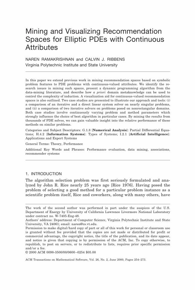
Example 2. We now present an example where the database involves asingle continuous-valued problem feature f and multiple algorithms. Tosimplify the analysis, we assume a discretization of the original data intoequidepth buckets such that each bucket satisfies the support constraint(which implies that all sequences of buckets will also satisfy the con-straint). We then proceed to find the range that maximizes the confidencemeasure. For example, Figure 5 indicates a continuous attribute dis-cretized into eight buckets of size 20 with each entry denoting the numberof times a certain algorithm was best (the support fraction is thus 20/160,or 12.5%). As discussed in Fukuda et al. [1996], Bentley’s linear-timealgorithm [Bentley 1986] can be used to find a contiguous range thatmaximizes the confidence. It scans the data from left to right, maintainsboth the range ending at the scan point as well as the best range seen sofar, and uses these ranges to incrementally compute the ranges for the nextscan point; see Manber [1992] for a description of this algorithm.

2.2 Two-Dimensional Mining

Extending this scheme to two dimensions (with more than one continuous-valued feature) is simple if the goal is to find a contiguous rectangularregion. The straightforward extension of the 1D case results in a O(N3)time algorithm (since there are N2 ways to choose the limits of therectangle and within each rectangle, the columns/rows can be collapsed toyield a 1D problem (which requires O(N) time)). A variation of thisapproach, popular in image processing and data mining [Fukuda et al.1996], is to allow nonrectangular regions whose intersection with a familyof isothetic axes (vertical or horizontal) is continuous. Such regions can befound in O(N2) time—an improvement over the regular rectangular algo-rithm. The technique makes use of a monotonicity property of connectedregions2 and is particularly appropriate for mining two-dimensional recom-mendation spaces, where confidence-optimizing regions are frequently non-rectangular.

Example 3. Consider a case with two continuous-valued attributes, f1and f2, where f1 varies in the range [0 . . . 25] and f2 varies in the range

2This is different from the antimonotonicity nature of the constraints used for data mining.

Fig. 5. A uniform bucketing of a continuous attribute. Each entry denotes the number oftimes a certain algorithm was best (out of a maximum of 20). The emphasized bucket range[4, 5] indicates the solution obtained by Bentley’s algorithm with a confidence of 0.6.



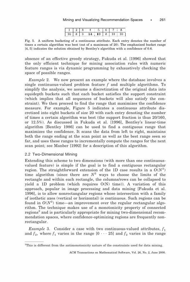
[0 . . . 1000]. The first step is to discretize these ranges into buckets (thiscan either be obtained from the process that generated the data or beachieved by equidepth sampling techniques). The goal of this step is toensure that all buckets satisfy a minimum support constraint. Let usassume that equidepth buckets are obtained for

f1 [ $@0, 5!, @5, 10!, @10, 15!, @15, 20!, @20, 25#%

f2 [ $@0, 1!, @1, 10!, @10, 100!, @100, 1000#%

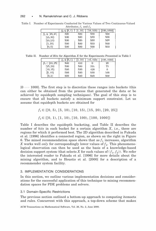
Table I describes the equidepth bucketing, and Table II describes thenumber of hits in each bucket for a certain algorithm X, i.e., these areregions for which it performed best. The 2D algorithm described in Fukudaet al. [1996] identifies a connected region, as shown on the right in Figure6. The mined recommendation space shows that as f1 increases, algorithmX works well only for correspondingly lower values of f2. This phenomeno-logical observation can then be used as the basis of a knowledge-baseddecision support system (that selects X for such values of ( f1, f2)). We referthe interested reader to Fukuda et al. [1996] for more details about themining algorithm, and to Houstis et al. [2000] for a description of arecommender system facility.

3. IMPLEMENTATION CONSIDERATIONS

In this section, we outline various implementation decisions and consider-ations for the successful application of this technique to mining recommen-dation spaces for PDE problems and solvers.

3.1 Domain-Specific Restrictions

The previous section outlined a bottom-up approach to computing itemsetsand rules. Concurrent with this approach, a top-down scheme that makes

Table I. Number of Experiments Conducted for Various Values of Two Continuous-ValuedAttributes, f1 and f2

Table II. Number of Hits for Algorithm X for the Experiments Presented in Table I



use of a priori domain metaknowledge can suggest directions to explore andcollect further data. This is the experiment generation problem studied inSubramanian and Feigenbaum [1986]. Examples of metaknowledge for thisdomain include the following:

—Factorization: If the recommendation space can be factored into multi-ple, independent recommendation subspaces. For example, if we knewthat the effects of feature f1 on algorithm applicability are completelyindependent of the effects of feature f2, we can attempt to learn twodifferent patterns (and combine them later) by a divide-and-conquerapproach. Subramanian et al. refer to such patterns as factorizableconcepts [Subramanian and Feigenbaum 1986]. Factorization can also beused to a limited extent if the features impose a hierarchical structure. Itcan also be applied to the case when both symbolic and numeric featureattributes are present.

—Subspace Elimination: If the recommendation space contains impossi-ble subspaces, due to semantic considerations arising from problemdefinition. For example, consider domain #20 from the population ofnonrectangular PDE domains defined by Rice [1984]. This domain in-volves two intersecting circles controlled by two continuous-valued pa-rameters. The radius of one of the circles is fixed at 1, while the otherradius is allowed to vary (which is the second parameter f2). In addition,the first parameter ( f1) controls the degree of overlap between the twocircles. This domain poses the constraint that the condition

f2 . Î1 2 f12

be satisfied for every valid PDE problem. Thus, data points belonging tosubspaces that do not satisfy this constraint need not even be evaluated.

Fig. 6. (left) The data in Table II modeled by a colormap that associates the confidencemeasure in each bucket with the intensity of pixels. Thus, the darker regions reflect a greaternumber of hits. (right) The confidence-optimizing region mined by the algorithm of Fukuda etal. [1996].



—Constraints: If the application domain poses constraints on the natureof the induced spaces. Consider again the recommendation space minedin Figure 6 where f2 has been shown to have a “staircase” effect on theapplicability of algorithm X with respect to feature f1. Modeling thisconstraint beforehand can assist in exploring the recommendation space.There are two main approaches to encoding such knowledge: (i) in thecontrol flow of the mining algorithm, or (ii) as declarative constraints inthe database environment. We prefer the latter which allows for the useof active and rule-based elements to aid in interactive exploration. Forinstance, the staircase constraint can be modeled via the rule base inFigure 7. The first line in Figure 7 indicates that if the bucket corre-sponding to ( f1, f2) is part of the recommendation space but not the oneto its right (( f1 1 1, f2)), then no bucket to the top of ( f1 1 1, f2) can bepart of the recommendation space, and so on.

—Selective Focusing: This facility is most useful when coupled withincremental computation of recommendation spaces by techniques suchas those described in Hidber [1999]. Assume that we obtain a “coarse”image of the recommendation space by specifying a moderate level ofsupport. One could then zoom in to regions that look promising withoutevaluating other portions of the space. Selective focusing is also facili-tated by database-sampling techniques that can dynamically prefetchdata based on user preferences [Hellerstein et al. 1999].

—Bootstrapping: If a recommendation space between features f1 and f2

has been computed for a coarse level of discretization (of the featurespace), the patterns mined from this space can be used to bootstrap thestudy for a finer level of discretization. We have actively utilized thisbootstrapping technique for many of the datasets presented in this paper.For example, if a 5 3 5 bucketing of the feature space reveals a spikealong the y-axis, bootstrapping the mining algorithm with this informa-tion can narrow down the search space for a higher level of discretization.Bootstrapping can also be employed when we move from a lower-dimen-sional feature space to higher dimensions.

3.2 Visualizing Recommendation Spaces

Since the mined recommendation spaces could be of arbitrary shape,visualization of the induced regions constitutes an important stage in this

Fig. 7. Declarative modeling of a staircase constraint for recommendation spaces, where thecomputations are performed w.r.t. bucket numbers. hit(f1, f2) is true if the bucketcorresponding to ( f 1, f 2) is a “hit,” false otherwise.



experimental mode of investigation (in contrast, purely symbolic attributesrestrict the mined regions to the corners of an m-dimensional featurehypercube). We have implemented a visualization facility using the Densi-tyGraphics and RGBColor primitives provided in Mathematica. Thesefunctions enable the creation of colormaps that map regions of the recom-mendation space to proportions of color components for pixels displayed ineach box. One such design is presented in Fukuda et al. [1996] and uses themapping f( x) 5 { x, 1 2 x, 0}, where each component of f( x) reflects thecomponents according to the RGB model ( x denotes the “hit ratio” for acertain algorithm). The advantages of this mapping are threefold: (i) it usesintensity to provide visual clues that aid in human perception of recommen-dation spaces; (ii) by setting the blue component to zero, it minimizes thenumber of colors required to provide acceptable discrimination; and (iii) thecolors are not too saturated that perception of detail is impossible. Apotential disadvantage of this approach is that it limits the number ofdifferent algorithms (choices) that can be represented in a single image.However, from our experiments, the efficiency of the visual search processis significantly enhanced by restricting this number to 2. This factorappears to be heavily application-dependent, and our observation mirrorsmany psychophysical studies of the use of color in identification tasks[Nowell 1997; Smallman and Boynton 1990]. An example of the f( x)mapping is depicted in the left part of Figure 6. The right part of Figure 6depicts the region automatically mined by the algorithm of Fukuda et al.[1996]. We use the mapping g( x) 5 {0, 0, 1} (“blue”) for the subregionsthat optimize confidence and g( x) 5 {1, 1, 1} (“white”) otherwise.

4. CASE STUDIES

In this section, we present two case studies which illustrate our approachto mining and visualizing recommendation spaces for PDEs with continu-ously varying parameters. The simple examples here do not necessarilyyield significant new insight into the behavior of particular numericalmethods, but rather suggest how this approach can be used in the PDEproblem-solving context. In both examples, we explore data sets involvinglinear, second-order, two-dimensional elliptic PDEs, discretized using stan-dard O(h2) accurate finite differences, with linear systems solved usingKrylov subspace solvers preconditioned with incomplete factorizations. Weconsider nonsymmetric problems with features that can often cause diffi-culties for iterative solvers. The first example explores the influence of oneproblem parameter and one method parameter on whether to use aniterative or a direct method. In the second example, we look for patterns inthe relative performance of two widely used iterative methods on problemsposed on a nonrectangular domain, with one problem parameter controllingthe shape of the domain and one influencing the PDE coefficients.

The framework used to carry out these case studies includes the ELL-PACK system [Rice and Boisvert 1985], SPARSKIT [Saad 1990], andseveral scripts which generate and process the data. A script generates an



ELLPACK program which defines a particular PDE problem and solutionmethod. The ELLPACK discretization module “5 point star ” is usedthroughout. SPARSKIT solvers gmres and bcgstab , and preconditionersilut and ilutp , were incorporated into ELLPACK and used as solvers andpreconditioners, respectively. All experiments were carried out on a500MHz Digital Alpha workstation.

4.1 Iterative or Direct Linear Solver?

One of the attractions of direct solution methods (e.g., Gaussian elimina-tion or one of its variants) for solving linear systems of equations is thatthey are essentially guaranteed to work. This “guarantee” ignores thepossibility of various numerical disasters, of course, as well as significantperformance problems that may stem from the nonzero structure of thematrix, the data structures used, memory hierarchy, etc. But nonetheless,it is true, especially for nonsymmetric problems, that iterative methodsintroduce a question direct methods do not, namely, “Will it converge?”, andif so, “In how much time?” Much is known theoretically about the conver-gence behavior of iterative methods on model problems. But for moregeneral problems, the choice of a good Krylov solver and preconditioner isoften made in an ad hoc manner. In this case study, we illustrate howmining a large database of already solved problems can yield helpfulinsight into the choice between iterative and direct methods.

Consider the scalar linear elliptic equation

2¹2u 1a

~b 1 x 1 y!2ux 1

a

~b 1 x 1 y!2uy 5 f~ x, y!,

with Dirichlet boundary conditions on the unit square, where b . 0 andf( x, y) is chosen so that the true solution is the smooth function

u~ x, y! 5 ~cos~ y! 1 sin~ x 2 y!! p ~1 1 sin~ x/ 2!!.

Discretized with centered (“five-point”) finite differences, this problemresults in a linear system that is increasingly ill-conditioned for large a andsmall b, respectively. The singularity in the operator is just outside thedomain, along the line b 1 x 1 y 5 0. We observed in preliminaryexperiments that the Krylov solvers have difficulty as this problem ap-proaches the singular case, i.e., as a /b2 grows. What is not so clear is howquickly the performance will degrade, and how much preconditioning canhelp.

We solved this problem using a uniform grid with spacing h 5 1/100,resulting in 9801 discrete equations and unknowns. We compared the timetaken by the ELLPACK band Gaussian elimination direct solver to thetime taken by a typical Krylov solver with fixed memory requirements,namely gmres(10) with ilutp preconditioning and a relative residualreduction of 1026. (The notation gmres(10) indicates gmres with a restartparameter of 10.) The ilutp preconditioner is a variant of ilut which uses



partial pivoting [Saad 1996, Chap. 10]. Both ilut and ilutp rely on a dualthresholding strategy controlled by two parameters, lfill and droptol .When constructing the preconditioner, these methods drop any elementwhose absolute value is less than droptol relative to the size of thediagonal element. At the same time, only the lfill largest off-diagonalelements in each row of the factors L and U are kept. In this way, lfill isused to limit the storage requirements of the preconditioner, while drop-tol is used to select only the largest elements for inclusion in thepreconditioner. Half of the data in this case study was generated withdroptol 5 0.0 and the other half with droptol 5 0.001. When droptol 50, the thresholding procedure essentially disappears, with no matrix ele-ments being thrown away because they are too small. The method thenreduces to the simple strategy of keeping the largest lfill elements oneach row of the factors L and U. For each of the two choices for droptol weset

b 5 0.01, 0.02, . . . , 0.05

lfill 5 2, 4, 6, . . . , 30

and let log10(a) vary randomly in [0, 3]. Each combination of the problemand solution parameters corresponds to a separate PDE solve—45,000 (5values of b 3 15 values of lfill 3 2 values of droptol 3 300 values of a)in all for this study. In this and the next study, we set the minimumsupport fraction such that every bucket satisfies the requirement.

In Figures 8 and 9 we show the results for a [ [1, 200], for droptol 5 0and droptol 5 0.001, respectively. The top row in Figure 8 shows the“hits” for gmres and a direct solve (left and right, respectively), where adarker shading means a higher percentage of wins for that method. In thebottom row of Figure 8, we show the results of the confidence-optimizingregion-mining algorithm for each method for a confidence level u 5 0.9. Theimportance of the parameter droptol is clearly seen. When droptol 5 0,lfill must fall within a relatively narrow interval in order for theiterative method to be preferred, and this is increasingly true as a in-creases. Eventually, for large enough a, the direct solve is always the bestmethod. In contrast, we see in Figure 9 that setting droptol 5 0.001makes ilutp much more robust with respect to changes in both a andlfill . In this case, as long as lfill is sufficiently large the iterativemethod is preferred. There is no penalty for choosing lfill too largebecause the droptol parameter ensures that less-important elements arenot kept, no matter how large lfill is. Furthermore, the results give someguidance regarding what a “sufficiently large” value for lfill might be, fora given a.



4.2 Which Iterative Method?

A second case study considers the relative performance of two well-knownKrylov solvers on problems posed on a nonrectangular region with a stepfunction in the PDE coefficients. The differential equation solved here is

2~w~ x, y!ux!x 2 ~w~ x, y!uy!y 5 2.0,

with homogeneous Dirichlet boundary conditions on the boundary of theregion V shown in Figure 10. This is Domain 20 from the populationdefined in Rice [1984]. Note that V is parameterized by p. The domainconsists of two overlapping circles of radius 1.0 which intersect at x 5 p.The coefficient w( x, y) is defined as a step function, taking on the value aif ( x, y) is in the region where the two circles overlap, and returning thevalue 1.0 otherwise.

Again we discretize using second-order accurate finite differences, thistime using a 151 3 151 uniform grid. The resulting systems of linear

Fig. 8. Case Study 1 results: relative frequency of hits for gmres (top left) and direct solve(top right); u 5 0.9 confidence regions for gmres (bottom left) and direct solve (bottom right),for droptol 5 0. Notice that the intersection of the region on the right with a horizontal orvertical segment can lead to a discontinuity; it was obtained by two consecutive runs of themining algorithm, i.e., once a region is obtained by the algorithm, the data corresponding tothis region is removed and the algorithm run again. The end result is a superposition of thetwo regions.



equations are of dimension approximately 18,500, the size varying slightlywith p. We compare the time taken by SPARSKIT’s gmres(10) and bcgstab ,both preconditioned with ilut . (We select restart parameter 10 for gmres sothat the storage requirements of the two iterative methods are approximatelythe same.) For this case study, droptol is fixed at 0.001 while lfill isallowed to vary. The results shown in Figures 11 and 12 are from a data setgenerated by letting p vary randomly in the interval [0.75, 0.95].

Fig. 9. Case Study 1 results: relative frequency of hits for gmres (top left) and direct solve(top right); u 5 0.9 confidence regions for gmres (bottom left) and direct solve (bottom right),for droptol 5 0.001.

Fig. 10. Domain for Case Study 2: p 5 0.5 (left) and p 5 0.9 (right).



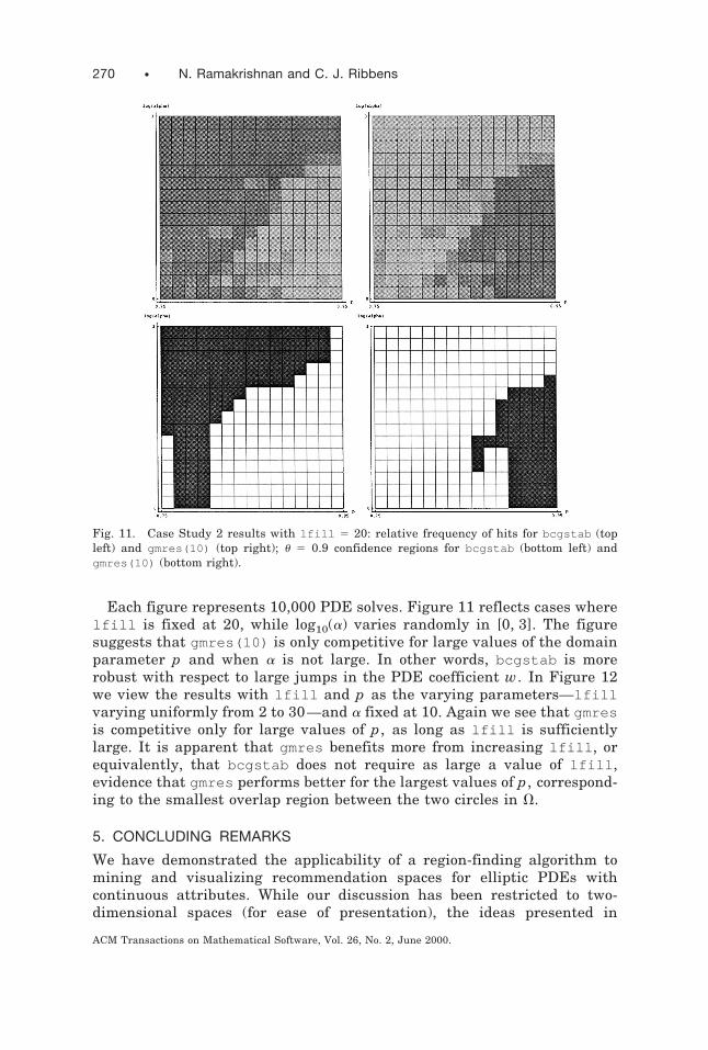
Each figure represents 10,000 PDE solves. Figure 11 reflects cases wherelfill is fixed at 20, while log10(a) varies randomly in [0, 3]. The figuresuggests that gmres(10) is only competitive for large values of the domainparameter p and when a is not large. In other words, bcgstab is morerobust with respect to large jumps in the PDE coefficient w. In Figure 12we view the results with lfill and p as the varying parameters—lfillvarying uniformly from 2 to 30—and a fixed at 10. Again we see that gmresis competitive only for large values of p, as long as lfill is sufficientlylarge. It is apparent that gmres benefits more from increasing lfill , orequivalently, that bcgstab does not require as large a value of lfill ,evidence that gmres performs better for the largest values of p, correspond-ing to the smallest overlap region between the two circles in V.

5. CONCLUDING REMARKS

We have demonstrated the applicability of a region-finding algorithm tomining and visualizing recommendation spaces for elliptic PDEs withcontinuous attributes. While our discussion has been restricted to two-dimensional spaces (for ease of presentation), the ideas presented in

Fig. 11. Case Study 2 results with lfill 5 20: relative frequency of hits for bcgstab (topleft) and gmres(10) (top right); u 5 0.9 confidence regions for bcgstab (bottom left) andgmres(10) (bottom right).



Section 3.1 can be used to scale up to higher dimensions. In addition, mostevaluation criteria for data-mining systems involve limitations that boundthe recommendation space from both above and below. Bayardo andAgrawal [1999] showed that the computation of the 2D range describedhere contains both a positive and a negative border. Thus, one couldmaintain two sets of patterns (at the expense of optimality), and updateeach set dynamically in opposite directions till the borders are reached.While we have not utilized this technique in this paper, we believe that thiswill be necessary in scaling up to more than two dimensions.

Our future work focuses on automating many aspects of the toolspresented here—dynamic selection of sampling criteria, using augmenteddata structures for in-core computations of large datasets, and moredetailed characterization of the scientific datasets that are particularlyamenable to such techniques. The encouraging results presented in thispaper arise from limiting the nature of the induced recommendationspaces. Various studies are planned to address the important issue ofknowledge compilation—“how to tractably represent/encode application-specific knowledge without compromising efficiency?”—within this frame-

Fig. 12. Case Study 2 results with a 5 10: relative frequency of hits for bcgstab (top left)and gmres(10) (top right); u 5 0.9 confidence regions for bcgstab (bottom left) andgmres(10) (bottom right). Notice again that the region on the right is obtained by twoconsecutive runs of the mining algorithm, as described earlier.



work. Finally, the results of the second case study give a hint that gmreshas an advantage over bcgstab as the outer iteration in an overlappingdomain decomposition (Schwarz) method, for example. Although the studywas designed to study the relationship between nonrectangular geometriesand iterative solvers in a rather general way, it is interesting that we areled to this possibility for future investigations into the relationship be-tween subdomain overlap and iterative methods.

REFERENCES

ADDISON, C., ENRIGHT, W., GAFFNEY, P., GLADWELL, I., AND HANSON, P. 1991. Algorithm 687:A Decision Tree for the Numerical Solution of Initial Value Ordinary Differential Equations.ACM Transactions on Mathematical Software Vol. 17, 1, pp. 1–10.

AGRAWAL, R., IMIELINSKI, T., AND SWAMI, A. 1993. Mining Association Rules Between Sets ofItems in Large Databases. Proceedings of the ACM SIGMOD Conference on Management ofData, pp. 207–216. Washington, D.C.

AGRAWAL, R., MANNILA, H., SRIKANT, R., TOIVONEN, H., AND VERKAMO, A. I. 1996. Fast Discoveryof Association Rules. In U. M. Fayyad, G. Piatetsky-Shapiro, P. Smyth, and R. UthurusamyEds., Advances in Knowledge Discovery and Data Mining. AAAI/MIT Press, Cambridge, MA.

BAYARDO, R. J., JR. AND AGRAWAL, R. 1999. Mining the Most Interesting Rules. Proceedingsof the ACM SIGKDD International Conference on Knowledge Discovery and Data Mining.

BENTLEY, J. L. 1986. Programming Pearls. Addison-Wesley.BOISVERT, R., RICE, J., AND HOUSTIS, E. 1979. A System for Performance Evaluation of

Partial Differential Equations Software. IEEE Transactions on Software Engineering Vol.SE-5, 4 (July), pp. 418–425.

DE STURLER, E. 1996. A Performance Model for Krylov Subspace Methods on Mesh-BasedParallel Computers. Parallel Computing 22, pp. 57–74.

FUKUDA, T., MORIMOTO, Y., MORISHITA, S., AND TOKUYAMA, T. 1996. Data Mining UsingTwo-Dimensional Optimized Association Rules: Schema, Algorithms and Visualization.Proceedings of the ACM SIGMOD Conference on Management of Data, pp. 13–23.

GREENBAUM, A. 1997. Iterative Methods for Solving Linear Systems. SIAM, Philadelphia.HAN, J., LAKSHMANAN, L. V. S., AND NG, R. T. 1999. Constraint-Based, Multidimensional

Data Mining. IEEE Computer 32, 8, pp. 46–50.HELLERSTEIN, J. M., AVNUR, R., CHOU, A., HIDBER, C., OLSTON, C., RAMAN, V., ROTH, T., AND HAAS,

P. J. 1999. Interactive Data Analysis: The Control Project. IEEE Computer 32, 8, pp. 51–59.HIDBER, C. 1999. Online Association Rule Mining. Proceedings of the ACM SIGMOD Con-

ference on Management of Data, pp. 145–156.HOUSTIS, E., RICE, J., WEERAWARANA, S., CATLIN, A., PAPCHIOU, P., WANG, K., AND GAITATZES, M.

1998. Parallel ELLPACK: A Problem Solving Environment for PDE Based Applications onMulticomputer Platforms. ACM Transactions on Mathematical Software 24, 1, pp. 30–73.

HOUSTIS, E. N., CATLIN, A. C., RICE, J. R., VERYKIOS, V. S., RAMAKRISHNAN, N., AND HOUSTIS,C. E. 2000. PYTHIA II: A Knowledge/Database System for Managing Performance Dataand Recommending Scientific Software. ACM Transactions on Mathematical Software.appears in this issue.

IMIELINSKI, T. AND MANNILA, H. 1996. A Database Perspective on Knowledge Discovery.Communications of the ACM, pp. 58–64.

KAMEL, M., MA, K., AND ENRIGHT, W. 1993. ODEXPERT: An Expert System to SelectNumerical Solvers for Initial Value ODE Systems. ACM Transactions on MathematicalSoftware 19, pp. 44–62.

LUCKS, M. AND GLADWELL, I. 1992. Automated Selection of Mathematical Software. ACMTransactions on Mathematical Software Vol. 18, 1, pp. 11–34.

MANBER, U. 1992. Introduction to Algorithms: A Creative Approach. Addison-Wesley.MITCHELL, T. M. 1982. Generalization as Search. Artificial Intelligence 18, 2, pp. 203–226.



NOWELL, L. T. 1997. Graphical Encoding for Information Visualization: Using Icon Color,Shape, and Size to Convey Nominal and Quantitative Data. Ph.D. thesis, Virginia Polytech-nic Institute and State University.

PARK, J. S., CHEN, M.-S., AND PHILIP, S. Y. 1995. An Effective Hash Based Algorithm forMining Association Rules. Proceedings of the ACM SIGMOD Conference on Management ofData, pp. 175–186.

POMMERELL, C. AND FICHTNER, W. 1994. Memory Aspects and Performance of IterativeSolvers. SIAM J. Sci. Comput. 15, pp. 460–473.

RAMAKRISHNAN, N. 1999. Experiences with an Algorithm Recommender System. In P. BaudischEd., Proceedings of the CHI’99 Workshop on Recommender Systems. ACM SIGCHI Press.

RAMAKRISHNAN, N. AND GRAMA, A. 1999. Data Mining: From Serendipity to Science. IEEEComputer 32, 8, pp. 34–37. Guest Editors’ Introduction to the Special Issue on Data Mining.

RAMAKRISHNAN, N. AND VALDES-PEREZ, R. E. 2000. Note on Generalization in ExperimentalAlgorithmics. ACM Transactions on Mathematical Software. to appear.

RIBBENS, C. J. AND RICE, J. R. 1986. Realistic PDE Solutions for Non-Rectangular Domains.Technical Report CSD-TR-639, Department of Computer Sciences, Purdue University, WestLafayette, IN.

RICE, J. 1976. The Algorithm Selection Problem. Advances in Computers 15, pp. 65–118.Academic Press, New York.

RICE, J. 1984. Algorithm 625: A Two-Dimensional Domain Processor. ACM Transactions onMathematical Software 10, pp. 453–462.

RICE, J., HOUSTIS, E., AND DYKSEN, W. 1981. A Population of Linear, Second Order, EllipticPartial Differential Equations on Rectangular Domains, Part I. Mathematics of Computa-tion 36, pp. 475–484.

RICE, J. R. AND BOISVERT, R. F. 1985. Solving Elliptic Problems Using ELLPACK. Springer-Verlag, New York.

SAAD, Y. 1990. SPARSKIT: A Basic Tool Kit for Sparse Matrix Computations. TechnicalReport 90-20, Research Institute for Advanced Computer Science, NASA Ames ResearchCenter, Moffet Field, CA.

SAAD, Y. 1996. Iterative Methods for Sparse Linear Systems. PWS Publishing, Boston.SARAWAGI, S., THOMAS, S., AND AGRAWAL, R. 1998. Integrating Association Rule Mining with

Relational Database Systems: Alternatives and Implications. Proceedings of the ACMSIGMOD Conference on Management of Data, pp. 343–354.

SCHMID, W., PAFFRATH, M., AND HOPPE, R. H. W. 1995. Application of Iterative Methods forSolving Nonsymmetric Linear Systems in the Simulation of Semiconductor Processing.Surv. Math. Indust. 5, pp. 1–26.

SMALLMAN, H. S. AND BOYNTON, R. M. 1990. Segregation of Basic Colors in an InformationDisplay. Journal of the Optical Society of America 7, 102, pp. 1985–1994.

STEINACHER, S. 1998. Data Mining: What Your Data Would Tell You if It Could Talk.http://news400.com.

SUBRAMANIAN, D. AND FEIGENBAUM, J. 1986. Factorization in Experiment Generation. Pro-ceedings of the National Conference on Artificial Intelligence (AAAI’86), pp. 518–522.

WEERAWARANA, S., HOUSTIS, E., RICE, J., JOSHI, A., AND HOUSTIS, C. 1996. PYTHIA: AKnowledge Based System to Select Scientific Algorithms. ACM Transactions on Mathemat-ical Software 22, pp. 447–468.

ZHANG, J. 1996. Preconditioned Krylov Subspace Methods for Solving Nonsymmetric Matri-ces from CFD Applications. Technical Report 280-98, Department of Computer Science,University of Kentucky, Lexington, KY. To appear in Computer Methods in AppliedMechanics and Engineering.

Received October 1999; revised March 2000 and May 2000; accepted May 2000



Date post:	01-Apr-2018
Category:	Documents
Upload:	leanh
View:	216 times
Download:	1 times

Mining and Visualizing Recommendation Spaces …people.cs.vt.edu/naren/papers/mine-viz.pdfMining and...

Documents