Mining Bad Credit Card Accounts from OLAP and OLTP Sheikh Rabiul Islam

Tennessee Technological University 1 William L Jones Dr Cookeville, TN 38505 +1 (931) 372-3101

sislam42@students.tntech.edu

William Eberle Tennessee Technological University

1 William L Jones Dr Cookeville, TN 38505 +1 (931) 372-3101

weberle@tntech.edu

Sheikh Khaled Ghafoor Tennessee Technological University

1 William L Jones Dr Cookeville, TN 38505 +1 (931) 372-3101

sghafoor@tntech.edu

ABSTRACT

Credit card companies classify accounts as a good or bad based on

historical data where a bad account may default on payments in the

near future. If an account is classified as a bad account, then further

action can be taken to investigate the actual nature of the account

and take preventive actions. In addition, marking an account as

“good” when it is actually bad, could lead to loss of revenue – and

marking an account as “bad” when it is actually good, could lead to

loss of business. However, detecting bad credit card accounts in

real time from Online Transaction Processing (OLTP) data is

challenging due to the volume of data needed to be processed to

compute the risk factor. We propose an approach which

precomputes and maintains the risk probability of an account based

on historical transactions data from offline data or data from a data

warehouse. Furthermore, using the most recent OLTP transactional

data, risk probability is calculated for the latest transaction and

combined with the previously computed risk probability from the

data warehouse. If accumulated risk probability crosses a

predefined threshold, then the account is treated as a bad account

and is flagged for manual verification.

CCS Concepts

• Information systems➝ Information systems

applications • Data mining➝ Collaborative filtering

Keywords

OLTP, Data warehouse, Risk Probability, Classifier, WEKA.

1. INTRODUCTION Credit cards are usually issued by a bank, business or other

financial institution that allows the holder to purchase goods and

services on credit. A person can have multiple credit cards from

different companies. Companies who provide credit scores suggest

card holders use multiple credit cards in order to increase their

credit score. A credit score is a three-digit number between 300 and

850 that indicate the creditworthiness of a person. The credit score

is used by lenders to determine someone’s credit worthiness for

various lending purposes.

A credit score can affect whether or not someone is approved for

credit as well as what interest rate they will be charged [6].

Recklessly using multiple credits card is one of the reasons that

someone is unable to pay their credit card bill on time, which can

eventually turn into long-term debt for the card holder. Other

reasons for being unable to pay their bill include job loss, health

issues, or an inability to work, which can eventually result in

“bankruptcy “. In any case, this becomes an issue for both the credit

card companies and the customer.

To address this problem, besides carefully evaluating the

creditworthiness of credit card applicants at the very beginning, the

credit card issuer needs to identify potential bad accounts that are

at the risk of going to bankruptcy over the life of their credit. From

the creditor’s side, the earlier the bad accounts are identified, the

lower the losses [7]. A system that can identify these risky accounts

in advance would help credit card companies to take preventive

actions. They could also potentially communicate information to

the account holder and provide suggestions for avoiding

bankruptcy.

Online Analytical Processing (OLAP) systems typically use

archived historical data from a data warehouse to gather business

intelligence for decision-making. On the other hand, Online

Transaction Processing (OLTP) systems, only analyze records

within a short window of recent activities - enough to successfully

meet the requirement of current transactions [8]. Older

transactional data are usually excluded from OLTP due to

performance requirements and usually archived in the data

warehouse. To compute the risk factor associated with an account

both historical transactional data and recent transactions should be

used to get a more accurate picture. In this paper, we propose a

framework that computes the risk factor of a credit card account

using both archived data from the data warehouse as well as recent

transactions from OLTP. In our framework, the risk probability

from the recent transactions is calculated using two methods:

Standard Transaction Testing along with Adaptive Testing. We

have validated our framework using a dataset from a German credit

company found publicly on the internet [5]. Our approach can be

used to predict whether an account is bad or good in real time as a

transaction occurs. Our approach can then be used by a credit card

company to take a more proactive action when it comes to verifying

transactions and a customer’s ability to pay.

The following section contains some of the related work. The

framework for our approach is described in section 3. Section 4

describes the data sources with data preparation and feature

extraction. Experiments, Standard Transaction Testing, and

Adaptive Testing are described in Section 5. Section 6 contains

results, and section 7 presents our conclusions and future work

2. RELATED WORK A significant amount of research has been done in the area of

financial fraud analysis and detection, especially in credit card

fraud detection. However, not much work has been done in the area

of working with transactional data from an OLTP system to predict

bad credit card accounts. The research work of [1] is a dynamic

model and mechanism to discover fraud detection system

limitations while existing fraud detections systems use some

predefined rules and scenarios or static models. In this instance,

their dynamic model updates rules periodically [1]. They use a

KDA clustering model which is a combination of three clustering

algorithms, k-means, DBSCAN and the Agglomerative clustering

algorithm, that are then represented together as a dynamic solution

[1]. However, with this approach, the accuracy obtained by KDA

modeling for online data is much less than that of the offline data.

In the work of [3], the authors discuss different methods on fraud

detection based on decision trees using gini impurity, information

gain and a binary decision diagram. In the work presented in [4], a

data mining approach is presented using transaction patterns for

credit card fraud detection where the spending pattern may change

anytime due to changes in income and preferences.

Figure 1. High Level Diagram of the Proposed Framework.

In the work of [7], the authors present a system to predict personal

bankruptcy by mining credit card data. In their application, each

original attribute is transformed either to a binary [good behavior

and bad behavior] categorical attribute or multivalued ordinal

[good behavior and graded bad behavior] attribute. Consequently,

they obtain two types of sequences, i.e., binary sequences and

ordinal sequences. Later they resort to a clustering technique for

discovering useful patterns that can help them to identify bad

accounts from good accounts. Their system performs well,

however, they only use single data sources, whereas the bankruptcy

prediction systems of credit bureaus use multiple data sources

related to creditworthiness.

In summary, most work targets credit card fraud detection and is

performed on offline data from a data warehouse. Our proposed

approach is novel in that it works on data from both OLTP and

OLAP systems.

3. PROPOSED FRAMEWORK Our proposed framework computes the risk factor of an account by

combining the risk probability from archived data in a data

warehouse with the risk probability of a current transaction from

OLTP. The risk probability from the archived data or data

warehouse is precomputed and is stored as summarized data. The

risk probability from OLTP is computed in real time as transactions

occur and combined with the precomputed risk to determine the

overall risk factor. Figure 1 shows the high-level diagram of our

proposed framework. Figure 2 shows the flowchart of our proposed

framework. Whenever a new transaction occurs in the OLTP

system, it is passed through a Standard Transaction Testing process

that checks whether the transaction deviates from any of standard

rules.

Figure 2. Proposed Framework Flowchart.

If the transaction passes the Standard Transaction Testing, then no

further testing is done and the system continues with the next

transaction. However, if the transaction fails the Standard

Transaction Testing, then the transaction is passed to the Adaptive

Testing process where customer specific measures are taken into

OLTP

Database Data

Warehouse

Offline Risk

Probability

R Offline

Online Risk

Probability

R Online

Total Risk Probability

R Total = R Online + R Offline

Offline

data

source

Online

data

source

Manual Verification

Data

Warehouse

Offline Risk

Probability

( R Offline )

A new transaction from

OLTP system

Online Risk

Probability( R Online )

Total Risk Probability

R Total = R Online + R Offline

Raised for

manual

verification

End. Restart for next OLTP transaction

Pass/Fail

Fail Pass

>Threshold Yes No

OLTP

Database

Standard Transaction

Testing

Adaptive Testing

account to measure the deviation and the risk probability from

online data. Calculating risk probability from offline data is

asynchronous to calculating risk probability from online data. It is

a one-time job and is done at the beginning while configuring the

system for our framework. When a transaction occurs in the OLTP

system, the combined risk probability is calculated for that

transaction which is stored and contributes to the risk probability

from offline data for the next transaction from the same account.

When we created the initial framework, we experimented with

various popular classifiers (e.g., Naïve Bayes, J48, Rotation Forest,

etc.) on the offline data. From our initial experiments, we

discovered that Random Forest returns the highest number of

correctly classified instances, as well as having the fastest

execution times. The result is a risk probability for the offline data.

Detail comparison of the result from the classifiers is discussed in

the result section.

We express risk probability from offline data as R Offline and the risk

probability form online data as R Online. . Risk probability from

online data and risk probability from offline data are combined to

get the combined risk probability (online + offline). We then

express our overall or total risk probability as RTotal, which is

equivalent to R Online + R Offline . After subsequent transactions for

the same account, the combined risk probability R Total of the current

transaction is combined with the offline risk probability for the

same account. If the combined risk probability is greater than the

threshold then the account is flagged for manual verification,

otherwise the process ends here and starts from the beginning for

the next transaction. We use a combined risk probability

interchangeably with an overall or total risk probability in rest of

this paper.

4. DATA

4.1 Data Sources Finding large and interesting sources of financial data is

challenging as these data are not made available to the research

community because of obvious privacy issues. In this work, we use

a dataset of a German credit company found publicly on the internet

for research purposes [5]. That data contains both a credit summary,

as well some anonymized detail information. There is summarized

account information of 1000 accounts with 24 features or attributes.

This is a labeled dataset where each account is labeled as good or

bad (1 or 0). Table 1 shows what were determined to be the

important features – a process that will be defined in the next

section.

OLTP data consists of actual, real-time, transaction data.

Unfortunately, a real transaction dataset that directly corresponds

to this offline (summary or profile) dataset is not currently available

to the research community. Therefore, in order to present a proof-

of-concept, we will list some of the real OLTP transactions taken

from the credit cards online portal [12], shown in Table 3, along

with example use cases, shown in Section 5, that demonstrate how

they might contribute to the risk possibility calculation.

4.2 Offline Data Preparation In order to process the data and apply our models, we will use the

publicly available machine learning tool WEKA [11]. WEKA

requires the input dataset in a format called ARFF. An ARFF file

is an ASCII text file that describes a list of instances sharing a set

of attributes. ARFF files have two distinct sections. The first

section is the header information that contains the relation names,

a list of attributes (the columns in the data), and their types. The

second section contains the data information [10]. We will use an

online conversion tool [9] to convert the offline data (account

summary and profile) into the ARFF format. We will then use the

ARFF file as input to WEKA for our experiments.

Table 1. Attributes from German credit dataset

Attribute Type Example value

Status of existing checking account

Qualitative No checking accounts, salary assignment for at least 1 year,

>=1000

Duration in month Numerical 12 months

Credit history Qualitative No credit taken, all credit paid duly,

Present

employment since

Qualitative <1 year, < 4 years

Personal status Qualitative Male: divorced/separated, Female: single/married

Present residence

since

Numerical 24 months

Age in years Numerical 28 years

Housing Qualitative Rent, own

Job Qualitative Skilled employee, self-

employed

Foreign Worker Qualitative Yes, no

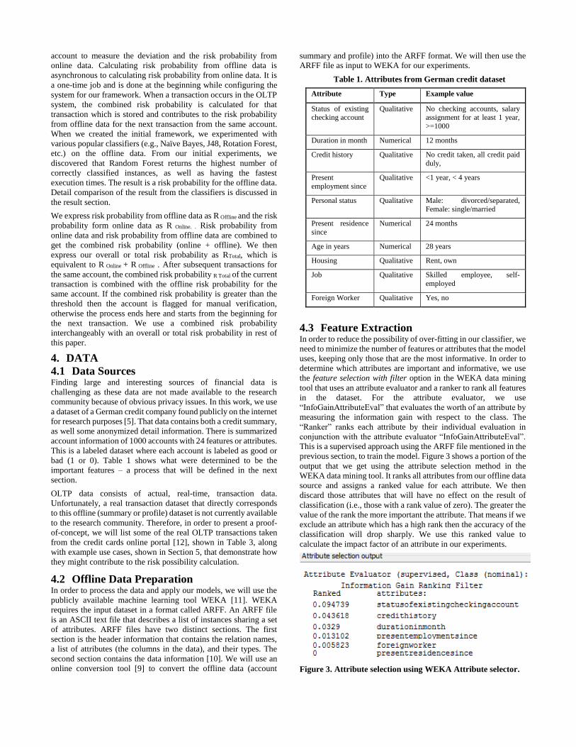
4.3 Feature Extraction In order to reduce the possibility of over-fitting in our classifier, we

need to minimize the number of features or attributes that the model

uses, keeping only those that are the most informative. In order to

determine which attributes are important and informative, we use

the feature selection with filter option in the WEKA data mining

tool that uses an attribute evaluator and a ranker to rank all features

in the dataset. For the attribute evaluator, we use

“InfoGainAttributeEval” that evaluates the worth of an attribute by

measuring the information gain with respect to the class. The

“Ranker” ranks each attribute by their individual evaluation in

conjunction with the attribute evaluator “InfoGainAttributeEval”.

This is a supervised approach using the ARFF file mentioned in the

previous section, to train the model. Figure 3 shows a portion of the

output that we get using the attribute selection method in the

WEKA data mining tool. It ranks all attributes from our offline data

source and assigns a ranked value for each attribute. We then

discard those attributes that will have no effect on the result of

classification (i.e., those with a rank value of zero). The greater the

value of the rank the more important the attribute. That means if we

exclude an attribute which has a high rank then the accuracy of the

classification will drop sharply. We use this ranked value to

calculate the impact factor of an attribute in our experiments.

Figure 3. Attribute selection using WEKA Attribute selector.

5. EXPERIMENTS For the purpose of calculating the risk probability from offline data,

we set up a classification experiment that gives the risk probability

for each account based on offline summary data. As mentioned

previously, we already have summarized information for 1000

accounts with their credit history. Among those, we use 50% of

these accounts to train the classifier and the remaining 50% to test

the classifier. We are interested in the probability value of being a

bad account or a good account for each of the accounts from the

classifiers results. This is the risk probability from the offline data

generated from the WEKA data mining tool. As mentioned

previous, we selected the Random Forest classifier as it provides

the best accuracy and execution time. So, using WEKA’s Random

Forest classifier, we calculate the risk probability of the offline

data. The classification gives us the binary result of each account

for being bad or good based on offline data. Random Forest

classifier gives us best results with a highest rate of correctly

classified instance of 74.6%. But we are not using that binary result

from classification. Instead, we are interested in the probability

value for each account being bad or good based on the offline data.

Random Forest also takes the lowest execution time .01 second to

classify provided 500 instances of test data.

We run all classifiers in WEKA 3.8.1 mostly using the default

parameters for all of the attributes unless otherwise specified. The

machine that we have used to do this experiment is a commodity

machine with 6GB RAM, Intel Core i5 CPU with a speed of 1.8

GHz. For Naïve Bayes, we choose the base version where all

default parameters were used. We used J48 classifier with pruning.

In the case of Random Forest, we set “breakTiesRandomly” to true

to break ties randomly when several attributes look equally good.

And for Rotation Forest, all default parameters were used. We then

take the probability value from the Random Forest as the value of

the risk probability from the offline data for each account. In

Section 6, we show the procedure of retrieving the offline risk

probability from the offline data. Figure 4 shows the probability

distribution of being a bad or good account based on offline data

for each of 500 accounts.

Figure 4. Probability distribution of offline data classification.

Figure 5 shows the density of probability instances. Here one

interesting thing is evident and that is for most of the instances, the

probability value tends to be in the upper or lower extremes rather

than in middle, leading to a more accurate overall risk probability

as values in the middle areas tend to show higher false positive

rates. For the purpose of getting the risk probability from online

data, we present our two methods: Standard Transaction Testing

and Adaptive Testing (as shown in Figure 2 and discussed in

Section 5). Remember, in order to be a real-time system, each new

transaction from the OLTP system is passed through this

framework as soon as the transaction occurs.

Figure 5. Instance Density.

5.1 Standard Transaction Testing The purpose of this test is to identify transactions that deviate from

the normal behavior and pass them to the next test named Adaptive

Testing. For the Standard Transaction Testing, we have made a

Standard Rule listing in Table 2. This is a partial collection of rules

that every normal or good transaction require to follow according

to our proposed framework. While this is just an initial set of rules

based on the perception, it is possible to add as many as rules

needed in this table based on future requirement. This Standard

Rules table contains all the rules that reflect standard and normal

behavior.

Table 2. Standard Rules

Rule ID Rule

1 Transaction amount < = Σ ( μ transaction amount + σ transaction

amount)

2 Number of transaction per day < = Σ ( μ number of transaction + σ number of transaction )

3 Payment within due date

4 Minimum amount due paid

5 Paid amount greater than or equal to due amount

6 Transaction location is near user’s physical location

The first rule we have in our table is, whether the transaction

amount is less than or equal to the summation of the average

transaction amount (μ transaction amount) and the standard

deviation of the transaction amount (σ transaction amount). The next

standard rule regards whether the number of transaction per day for

an account is less than or equal to the summation of the average

number of transactions per day per account (μ number of transaction)

and the standard deviation of the number of transactions per day

per account ( σ number of transaction). This can help in identifying

risky transactions. Other standard rules are included to indicate a

common set of rules, and are self-explanatory. Each new

transaction from the OLTP system is validated according to the

standard rules defined in Table 2. The flexibility of our proposed

approach allows for users to add as many standard rules as needed.

In summary, the Standard Rules perform the primary screening of

transactions.

We have collected some real OLTP credit card transactions to

explain the OLTP risk probability calculation. We have

anonymized the account number and transaction number for those

transactions. Though accounts for these OLTP transactions have no

direct mapping with the accounts of the offline data that we have.

As we couldn’t find a dataset comprises of both online and offline

data for the same set of accounts. Still, we have selected these

OLTP transactions very carefully to show a realistic relation among

both online and offline data.

Table 3. OLTP Transaction

TID AC Tran. Date

Description Amount ($)

Category

1 1 2017-01-20

SOUTHWES5268506576536 800-435-9792 TX

237.90 Airlines

2 2 2017-01-20

INTERNET PAYMENT - THANK YOU

25.00 Payments and Credits

3 3 2017-01-20

DNH*GODADDY.COM 480-505-8855 AZDNH*GODADDY.COM

155.88 Merchandise

4 4 2017-01-20

WM SUPERCENTER #657 COOKEVILLE TN

102.88 Supermarkets

5 5 2017-01-20

BESTBUYCOM775203010161 888-BESTBUY MN

131.69 Merchandise

Here, TID = Transaction Id, AC = Account Number and Tran.

Date= Transaction Date. From Table 3, we can see that, there is a

transaction for account number (AC) 1 with transaction id (TID) 1.

And it is a transaction of $237.90 for an air ticket purchase from

Southwest airlines. As soon as the transaction occurrs, it is passed

to the Standard Transaction Testing. All rules of Standard

Transaction Testing are not applicable to all transactions. There is

a relevance mapping table that contains which standard transaction

is relevant to which type of transaction. Here the type of the

transaction is determined by the category of the transaction. For the

first OLTP transaction, the “Air ticket purchase of $237.90”

relevancy mapping and satisfactory result is listed in the table

(Table 4).

If any rows of the relevancy table (Table 4) have the value “Yes”

in the “Relevancy” field for a transaction, it means that the

transaction is relevant to the rule. In a similar fashion, if the value

of the “Satisfy” field is “Yes”, the transaction satisfies the rule.

Now we check to see if rules for which the transaction under test is

relevant (Relevancy=Yes) but doesn’t satisfy (Satisfy=No) the rule.

That means to search for rows in Table 4 those have the value “Yes”

in “Relevancy” column but “No” in the satisfy column. If we can

find any such row, then the transaction has failed to pass the

Standard Transaction Testing. As we can see from the table (Table

4), row 1 and row 4 has the value “Yes” in the “Relevancy” field

but “No” in the “Satisfy” field. Thus, in this example, the

transaction has failed to pass the Standard Transaction Testing and

will need to be forwarded to the next test, Adaptive Testing, with a

reference that the transaction has failed to satisfy Rule ID 1 and 4

of the Standard Rules table (Table 2).

Table 4. Relevancy Mapping

Rule ID Rule Relevancy Satisfy

1 Transaction amount < = Σ ( μ

transaction amount + σ transaction amount) Yes No

2 Number of transaction per day < = Σ ( μ number of transaction + σ

number of transaction )

Yes Yes

3 Payment within due date No NA

4 Minimum amount due paid Yes No

5 Paid amount greater than or equal to due amount

No NA

6 Transaction location is near user’s physical location

Yes Yes

5.2 Adaptive Testing The Adaptive Testing process is a test that is more customer centric

rather than the standard rules that are applicable for every account

in the same way. It takes customer specific measures like foreign

national, job change, address change, promotion, salary increase,

etc. into consideration. This is a kind of test that recognizes possible

causes for which a transaction is unable to satisfy a rule in the

Standard Rules. Table 5 represents a listing of some of the possible

causes for which a transaction may fail to follow the relevant

standard rules in Table 2.

There are two new columns in Table 5: “Impact” and “Impact

coefficient”. Attributes found by the WEKA Attribute Selector tool

from the offline data described in the feature extraction section

gives us a ranked value (Fig. 3) for each attribute. Based on this

ranked value, and based on the relationship between an attribute

and related rules, we compute the impact associated with each

rule/cause, as specified in the “Impact” column of the table (Table

5). For example, a foreign worker is an attribute in our offline data,

and the causes “Out of the country” and “Air ticket purchase” of

Adaptive Testing are related to this attribute. This impact

assignment is completely company specific and customizable

based on different analysis. And impact coefficient is the

coefficient of the impact. Attributes those have more information

gain, we are assigning more impact to the causes related to those

attributes. Still a company may want to give more importance on

some adaptive causes than others based on the business

requirement. By default, this impact assignment is based on the

rank of the attribute and the relation of adaptive cause with the

attributes. Though companies have the provision to overwrite the

default impacts.

Returning to our previous example of a transaction of $237.90 for

the air ticket purchase by Account “1”, the transaction fails to pass

the Standard Transaction Testing due to two reasons 1) transaction

amount was above the summation of average transaction amount

and the standard deviation of the transaction amount, and 2)

minimum due of last month was unpaid. The transaction is then

passed to the Adaptive Testing component, along with the offending

rules from Table 2 (i.e., Rule ID 1, 4). The Adaptive Testing

component then checks its rules table for all rules that contain the

value 1 and/or 4 in its “Related Standard Rule” column (as shown

in Table 5).

Table 5. Adaptive Rules

Rule/ Cause ID

Rule/Cause Related Standard Rule

Impact Impact coefficient

1 Address change

6 1x 1

2 Air ticket purchase

1,2 1x 1

3 Job switch 3 2x 2

4 Out of the country

3,4,1,6 2x 2

5 Foreign Worker

3 2x 2

From Table 5, we can see that Rule/Cause ID 2 and 4 have the value

1 and/or 4 in their “Related Standard Rule” column, meaning that

the rules in row 2 and 4 are possible causes of breaking rules 1 and

4 of the Standard Rules (Table 2). So, we have got two possible

causes: 1) air ticket purchase, and 2) out of the country for breaking

the rule. In this case, the customer bought the air ticket but was not

out of the country. Now we will explain the risk probability

associated with this example (and others).

6. RESULTS To get the offline risk probability, we run the Random Forest

classifier on the offline data and take the risk probability value

associated with each of each account. To recall, Random Forest

gave us the highest correctly classified instances of 74.6% with the

lowest execution time of .01 seconds. Table 6 shows the result from

the top 4 classifiers for our experiment in terms of CCI and

execution time.

Table 6. Classifier Results on Offline Data

Cls CCI

%

ICI

%

Avg.

TP

Rate

Avg.

FP

Rate

Pr Re Time

Naïve

Bayes

73.8 26.2 .738 .43 .723 .762 .02

Rando

m

Forest

74.6 25.4 .75 .48 .733 .75 .01

Rotati

on

Forest

73.8 26.2 .738 .466 .721 .738 .02

J48 69.4 30.6 .694 .476 .676 .694 .01

Here,

CCI = Correctly Classified Instances

ICI = Incorrectly Classified Instances

Avg. TP Rate = TP/P

Avg. FP Rate = FP/N

Cls = Classifier

Pr = Precision

Re = Recall

Recall tells us how good a test is at detecting the positives, and

Precision tells us how many positively classified instances were

relevant. The “probability distribution” column in Figure 6 shows

the probability values of an account to be bad or good, which is the

offline risk probability for a particular account at the beginning.

This is a snapshot from WEKA’s Random Forest classifier on our

offline data. For instance, in row 4 of Figure 6, there is 87.9%

probability that the account is good and there is 12.1% probability

that the account is bad. Here, “instance #” is the account number

and “probability distribution” is the more granular result for that

account rather than just the binary result good or bad.

Figure 6. Probability distribution (from classification result)

on offline data.

As we said before that our online data and offline data are not

actually correlated. For the purpose of calculating overall risk

probability, we need to establish a correlation among them. For that

purpose, we are picking 5 random accounts and their offline risk

probability from offline data (Table 7) and then assigning account

number 1 to 5 to make a correlation with our online data.

Table 7. Offline (preprocessed) risk probability

Account Number Risk Probability from classification (%)

1 70

2 23

3 82

4 79

5 43

Total risk probability for a transaction comes from both online and

offline data. So, the equation of total risk probability is as below:

R Total = R Online + R Offline (1)

Here,

R Total = Overall risk probability from both online and offline data.

R Online = Risk probability from online data

R Offline = Risk probability from offline data

Furthermore, risk probability from online data and offline data may

carry different weights. For example, giving 60% weight to offline

data and 40% weight to online data might provide better mining

results for a particular company. On the other hand, for another

company, a different combination of offline vs online risk

probability weight might be better. So, the modified version of (1)

for a total risk probability calculation is:

R Total = λ R Online + (1- λ) R Offline (2)

Where λ is the risk factor.

For our experiments, we are assuming that a 70% weight from

online data and 30% weight from offline data which is an

established ratio by the long-term tuning of our system for better

mining results. So, for our case λ =.7 and 1- λ =.3. Data from both

sources are more or less important for the total risk analysis. And

this ratio can be adjusted based on trend analysis.

We can get the risk probability from offline data (R Offline) for

corresponding accounts from Table 7, which is related to the

instance risk probability distribution value of classification results.

To calculate the risk probability from online data (R Online), we have

derived the following equation:

R Online = [ 1 – Σ Impact Coefficient ( 𝑋)

Σ Impact Coefficient ( 𝑌) ] × 100 (3)

Where X = Relevant valid rules from the Adaptive Rules table

(Table 5) and Y = Relevant valid or invalid rules from the Adaptive

Rules table (Table 5)

In other words, X is the collection of rules from Adaptive Rules

table (Table 5) where the “Related Standard Rule” column has the

value of any of the rule ids that are passed from Standard

Transaction Testing and are valid causes for breaking a standard

rule; and Y is the collection of rules from the Adaptive Rules table

(Table 5) where the “Related Standard Rule” column has the value

of any of the rule ids that are passed from Standard Transaction

Testing irrespective of whether it is valid cause or not a valid cause.

If no rule/cause is found in Adaptive Rules table (Table 5) for a

transaction that is passed to Adaptive Testing, then the values of X

and Y become zero. Thus, the value of R Online from (3) becomes

100%, which means the customer has no customer specific reason

in the Adaptive Rule table resulting from assigning the highest

online risk probability possible for that transaction. If there were

some customer specific reasons, R Online would reduce by some ratio

based upon the number of customer specific causes/rules available

and the number of causes/rules among them that are valid for that

transaction.

Using the example presented earlier, customer with id 1 has bought

an air ticket but the customer is not out of the country or state yet.

Rule id 1 and rule id 4 from standard rule table (Table 2) were

relevant to the transaction but not satisfied. That’s why the

transaction was passed to “Adaptive Testing” with a reference to

rule id 1 and 4. In the Adaptive Test, from Table 5 it is found that

the row with “Rule/ Cause ID” 2 and 4 have the value 1 and or 4

in the “Related Standard Rule” column. So, either of rules out of

the country or Air ticket purchase from the adaptive rules table

(Table 5) is the cause of breaking the standard rules 1 and 4 for the

transaction we are explaining. That gives us:

Y ={ Out of the country, Air ticket purchase}

But the customer’s most recent location, which is usually appended

with the OLTP transaction description, says that the customer is not

out of the country (yet). So actually, out of the country is not a

valid reason for breaking the standard rules, though it is relevant.

Thus, with X ={ Air ticket purchase }, using the equation (3):

R Online =[ 1 - Σ Impact Coefficient ( 𝑋)

Σ Impact Coefficient ( 𝑌) ] × 100

=[1- Σ Impact Coefficient (Air ticket purchase)

Σ Impact Coefficient ( Air ticket purchase)+Impact Coefficient ( Out of the country) ]×100

= [ 1 - 1

1+2 ] ×100

= .67 × 100

= 67

From Table 7, we can see that offline risk probability for account 1

is 70%

So, R Offline = 70.

Putting these values in equation (2) and applying risk factors(λ) we

get the overall risk probability for account 1 after the transaction 1

is recorded in the OLTP system. Thus, the risk factors(λ) is .7 for

our case.

R Total = λ R Online + (1- λ) R Offline

= .7 × 67 + .3 × 70

= 67.9

So, for the transaction that we are explaining, there is a chance of

67.9% that this account is going to be a bad account.

For the proof-of-concept, we are assuming a Minimum Total Risk

Probability Threshold of 60% is established beforehand (by the

user) based on the analysis of historical data. This means that if the

total or overall risk probability is above 60%, then that transaction

will be treated as a risky transaction (along with the associated

account). In this example, the Overall Risk Probability (R Total) is

67.9% and that is above the threshold 60%, so the account for that

air ticket purchase transaction (Transaction 1) is suspended and

raised for manual verification to justify the actual nature of the

account.

When the overall risk probability for a transaction is completed, the

offline risk probability is adjusted based on the value of R Total,

which affects the offline risk probability value of the next

transaction for the same account. By this way, offline risk

probability for an account gradually increases if the customer

repeats similar transactions that are passed to the adaptive test from

the standard testing. The risk probability threshold of 60% is not

the only thing to consider. Besides the above tests, we are also

interested to know how much the transaction being analyzed

deviates from the median value. This will give us an idea of the

deviation intensity of the transaction in terms of its risk probability.

There is a precomputed median risk probability for each type of

transaction over some period of time from both sources of data that

is calculated separately from both Online and Offline data. The

overall median risk probability is calculated simply by adding the

online and offline median risk probability. Table 8 below lists the

process of calculating the deviation from the median. We compare

calculated risk probability for the transaction under experiment

with the median risk probability value of that type of transaction in

the case of online, offline and overall. The difference between them

is called the gap, as shown in Table 8.

Table 8. Calculating Gap

Online Offline Overall

Median risk

probability

of similar

transaction

M1 M2 M3

Risk

probability

of

Transaction

under

experiment

L1 L2 L3

Gap X=L1-M1 Y=L2-M2 Z=L3-M3

If any of either X, Y, Z from Table 8 is greater than zero, we signal

the transaction for manual verification and postpone activity of that

account.

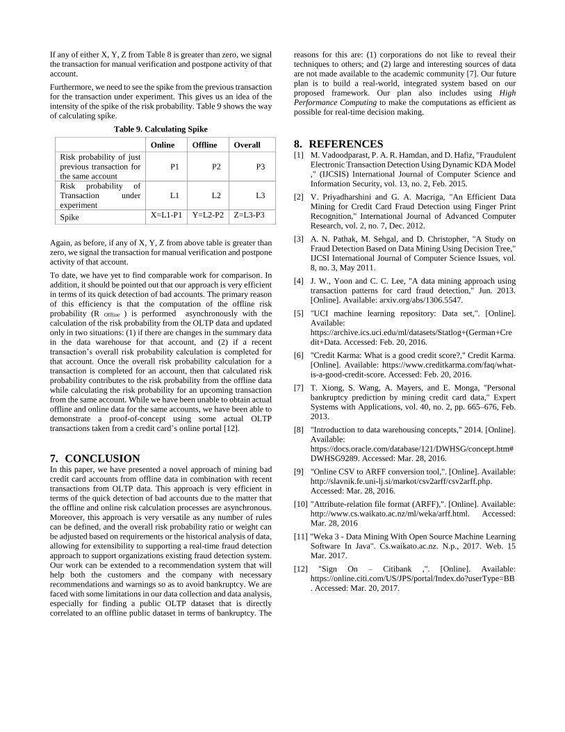
Furthermore, we need to see the spike from the previous transaction

for the transaction under experiment. This gives us an idea of the

intensity of the spike of the risk probability. Table 9 shows the way

of calculating spike.

Table 9. Calculating Spike

Online Offline Overall

Risk probability of just

previous transaction for

the same account

P1 P2 P3

Risk probability of

Transaction under

experiment

L1 L2 L3

Spike X=L1-P1 Y=L2-P2 Z=L3-P3

Again, as before, if any of X, Y, Z from above table is greater than

zero, we signal the transaction for manual verification and postpone

activity of that account.

To date, we have yet to find comparable work for comparison. In

addition, it should be pointed out that our approach is very efficient

in terms of its quick detection of bad accounts. The primary reason

of this efficiency is that the computation of the offline risk

probability (R Offline ) is performed asynchronously with the

calculation of the risk probability from the OLTP data and updated

only in two situations: (1) if there are changes in the summary data

in the data warehouse for that account, and (2) if a recent

transaction’s overall risk probability calculation is completed for

that account. Once the overall risk probability calculation for a

transaction is completed for an account, then that calculated risk

probability contributes to the risk probability from the offline data

while calculating the risk probability for an upcoming transaction

from the same account. While we have been unable to obtain actual

offline and online data for the same accounts, we have been able to

demonstrate a proof-of-concept using some actual OLTP

transactions taken from a credit card’s online portal [12].

7. CONCLUSION In this paper, we have presented a novel approach of mining bad

credit card accounts from offline data in combination with recent

transactions from OLTP data. This approach is very efficient in

terms of the quick detection of bad accounts due to the matter that

the offline and online risk calculation processes are asynchronous.

Moreover, this approach is very versatile as any number of rules

can be defined, and the overall risk probability ratio or weight can

be adjusted based on requirements or the historical analysis of data,

allowing for extensibility to supporting a real-time fraud detection

approach to support organizations existing fraud detection system.

Our work can be extended to a recommendation system that will

help both the customers and the company with necessary

recommendations and warnings so as to avoid bankruptcy. We are

faced with some limitations in our data collection and data analysis,

especially for finding a public OLTP dataset that is directly

correlated to an offline public dataset in terms of bankruptcy. The

reasons for this are: (1) corporations do not like to reveal their

techniques to others; and (2) large and interesting sources of data

are not made available to the academic community [7]. Our future

plan is to build a real-world, integrated system based on our

proposed framework. Our plan also includes using High

Performance Computing to make the computations as efficient as

possible for real-time decision making.

8. REFERENCES [1] M. Vadoodparast, P. A. R. Hamdan, and D. Hafiz, "Fraudulent

Electronic Transaction Detection Using Dynamic KDA Model

," (IJCSIS) International Journal of Computer Science and

Information Security, vol. 13, no. 2, Feb. 2015.

[2] V. Priyadharshini and G. A. Macriga, "An Efficient Data

Mining for Credit Card Fraud Detection using Finger Print

Recognition," International Journal of Advanced Computer

Research, vol. 2, no. 7, Dec. 2012.

[3] A. N. Pathak, M. Sehgal, and D. Christopher, "A Study on

Fraud Detection Based on Data Mining Using Decision Tree,"

IJCSI International Journal of Computer Science Issues, vol.

8, no. 3, May 2011.

[4] J. W., Yoon and C. C. Lee, "A data mining approach using

transaction patterns for card fraud detection," Jun. 2013.

[Online]. Available: arxiv.org/abs/1306.5547.

[5] "UCI machine learning repository: Data set,". [Online].

Available:

https://archive.ics.uci.edu/ml/datasets/Statlog+(German+Cre

dit+Data. Accessed: Feb. 20, 2016.

[6] "Credit Karma: What is a good credit score?," Credit Karma.

[Online]. Available: https://www.creditkarma.com/faq/what-

is-a-good-credit-score. Accessed: Feb. 20, 2016.

[7] T. Xiong, S. Wang, A. Mayers, and E. Monga, "Personal

bankruptcy prediction by mining credit card data," Expert

Systems with Applications, vol. 40, no. 2, pp. 665–676, Feb.

2013.

[8] "Introduction to data warehousing concepts," 2014. [Online].

Available:

https://docs.oracle.com/database/121/DWHSG/concept.htm#

DWHSG9289. Accessed: Mar. 28, 2016.

[9] "Online CSV to ARFF conversion tool,". [Online]. Available:

http://slavnik.fe.uni-lj.si/markot/csv2arff/csv2arff.php.

Accessed: Mar. 28, 2016.

[10] "Attribute-relation file format (ARFF),". [Online]. Available:

http://www.cs.waikato.ac.nz/ml/weka/arff.html. Accessed:

Mar. 28, 2016

[11] "Weka 3 - Data Mining With Open Source Machine Learning

Software In Java". Cs.waikato.ac.nz. N.p., 2017. Web. 15

Mar. 2017.

[12] "Sign On – Citibank ,". [Online]. Available:

https://online.citi.com/US/JPS/portal/Index.do?userType=BB

. Accessed: Mar. 20, 2017.