Mining Market Basket Data Using Share Measures and Characterized Itemsets Robert J. Hilderman, Colin L. Carter, Howard J. Hamilton, and Nick Cercone Department of Computer Science University of Regina Regina, Saskatchewan, Canada, $4S 0A2 {hilder,carter,hamilton,nick}@cs.uregina.ca Abstract. We propose the share-confidence framework for knowledge discovery from databases which addresses the problem of mining item- sets from market basket data. Our goal is two-fold: (1) to present new itemset measures which are practical and useful alternatives to the com- monly used support measure; (2) to not only discover the buying patterns of customers, but also to discover customer profiles by partitioning cus- tomers into distinct classes. We present a new algorithm for classifying itemsets based upon characteristic attributes extracted from census or lifestyle data. Our algorithm combines the Apriori algorithm for discov- ering association rules between items in large databases, and the AOG algorithm for attribute-oriented generalization in large databases. We suggest how characterized itemsets can be generalized according to con- cept hierarchies associated with the characteristic attributes. Finally, we present experimental results that demonstrate the utility of the share- confidence framework. 1 Introduction Consider a retail sales operation with a large inventory consisting of many dis- tinct products. The operation is situated in a location where the customer base is socio-economically diverse, with annual household incomes ranging from very low to very high, and demographically ranging from young families to the el- derly. The sales manager has used data mining to determine those products that are typically purchased together and those that are most likely to be pur- chased given that particular products have already been selected (called item- sets [2, 14]). Analysis of the itemsets has enabled him to strategically arrange store displays and plan advertising campaigns to increase sales. He now wonders whether there are any more subtle socio-economic buying patterns that could be helpful in guiding the distribution of flyers during the next advertising cam- paign. For example, he would like to know which itemsets are more likely to be purchased by those with specific incomes or by those with children. He would also like to know which itemsets are more likely to be purchased by those liv- ing in particular neighborhoods. He believes that characterizing itemsets with classificatory information available from credit card or cheque transactions will allow him to answer queries of this kind.
Transcript
Mining Market Basket Data Using Share Measures and Characterized I temsets
Robert J. Hilderman, Colin L. Carter, Howard J. Hamil ton, and Nick Cercone Department of Computer Science
University of Regina Regina, Saskatchewan, Canada, $4S 0A2
{hilder,carter,hamilton,nick}@cs.uregina.ca
Abs t r ac t . We propose the share-confidence framework for knowledge discovery from databases which addresses the problem of mining item- sets from market basket data. Our goal is two-fold: (1) to present new itemset measures which are practical and useful alternatives to the com- monly used support measure; (2) to not only discover the buying patterns of customers, but also to discover customer profiles by partitioning cus- tomers into distinct classes. We present a new algorithm for classifying itemsets based upon characteristic attributes extracted from census or lifestyle data. Our algorithm combines the Apriori algorithm for discov- ering association rules between items in large databases, and the AOG algorithm for attribute-oriented generalization in large databases. We suggest how characterized itemsets can be generalized according to con- cept hierarchies associated with the characteristic attributes. Finally, we present experimental results that demonstrate the utility of the share- confidence framework.
1 I n t r o d u c t i o n
Consider a retail sales operation with a large inventory consisting of many dis- tinct products. The operation is si tuated in a location where the customer base is socio-economically diverse, with annual household incomes ranging from very low to very high, and demographically ranging from young families to the el- derly. The sales manager has used da ta mining to determine those products that are typically purchased together and those that are most likely to be pur- chased given that particular products have already been selected (called item- sets [2, 14]). Analysis of the itemsets has enabled him to strategically arrange store displays and plan advertising campaigns to increase sales. He now wonders whether there are any more subtle socio-economic buying pat terns that could be helpful in guiding the distribution of flyers during the next advertising cam- paign. For example, he would like to know which itemsets are more likely to be purchased by those with specific incomes or by those with children. He would also like to know which itemsets are more likely to be purchased by those liv- ing in particular neighborhoods. He believes that characterizing itemsets with classificatory information available from credit card or cheque transactions will allow him to answer queries of this kind.
160
In this paper, we propose the share-confidence framework that looks beyond the simple frequency with which two or more items are bought together. We introduce a new algorithm, called CI, which integrates the Apriori algorithm for discovering association rules between items in large databases [2, 1], and the AOG algorithm for attribute-oriented generalization in large databases [9, 11]. We also show how market basket data can be mined using share measures and characterized itemsets which have been generalized according to concept hierarchies associated with characteristic attributes. However, it should be noted that our methods are not limited to the discovery of customer profiles based upon market basket data, the method is more widely applicable to any problem where taxonomic hierarchies can be associated with characterized data.
The remainder of this paper is organized as follows. In Section 2, we present a formal description of the market basket analysis problem and introduce the share-confidence framework. In Section 3, we describe characterized itemsets and an algorithm for generating characterized itemsets from market basket data. In Section 4, we present experimental results obtained using the share-confidence framework on a database supplied by a commercial partner. We conclude in Section 5 with a summary of our work.
2 T h e S h a r e - C o n f i d e n c e F r a m e w o r k
The problem of discovering association rules form market basket data has been formally defined as follows [2]. Let I = {il, i2 , . . . , ira} be a set of literals, called items. Let D be a set of transactions, where each transaction T is an itemset such that T C_ I. Transaction T contains X, a set of some items in I, if X C_ T. An association rule is an implication of the form X =~ Y, where X C I, Y C I, and X Cl Y = 0. The association rule X =~ Y holds in transaction set D with confidence c, if c% of transactions in D that contain X, also contain Y. The association rule X =~ Y has support s in transaction set D, if s% of transactions in D contain X U Y. This formalism is the support-confidence framework [4].
The most studied and analyzed algorithm for generating itemsets in the support-confidence framework is Apriori, described in detail in [1, 2, 3]. This algorithm extracts the set of frequent itemsets from the set of candidate item- sets generated. A frequent itemset is an itemset whose support is greater than some user-specified minimum and a candidate itemset is an itemset whose sup- port has yet to be determined. Apriori combines the frequent itemsets from pass k - 1 to create the candidate itemsets in pass k. It has the important property that if any subset of a candidate itemset is not a frequent itemset, then the candidate itemset is also not a frequent itemset.
In the support-confidence framework, the purchase of an item is indicated by a binary flag (i.e., the item is either purchased or not purchased). From this binary flag, we can determine the number of transactions containing an itemset, but not the number of items in the itemset. If we know the number of items, we may find that an itemset is actually more frequent than support indicates, allowing for more accurate financial analysis, comparisons, and projections. Since
161
support does not consider quantity and value, its use is limited as a practical indicator for determining the financial implications of an itemset.
We will now extend the formalization of the market basket problem. The problem definition is identical to that for the support-confidence framework, except that we introduce the notion of share for itemsets, and redefine the notions of frequent i temsets and confidence. We refer to this extended formalism as the share-confidence framework, introduced in [8] as share measures.
In the sections that follow, we define the functions upon which the share- confidence framework is based. For the examples, refer to the transaction database shown in Table 1 and the i tem database shown in Table 2. In Table 1, the TID column describes the transaction identifier and columns A to F describe the items (products) being sold. Note that binary values are not used to indicate the purchase of an item, instead the actual number of items purchased in the corresponding transaction (i.e., the counts) is used. In Table 2, the Item column describes the valid items and the Retail Price column describes the retailer 's selling price to the customer.
T a b l e 1. An example transaction database with counts ITID[A I NI CIDIE I FI
The definitions in this section were implemented in a da ta mining sys tem for analyzing market basket data. This system is an extension of DB-Discover, a software tool for knowledge discovery from databases [7, 6]. Definitions 1 to 6 are used to query summary views containing discovered frequent itemsets.
D e f i n i t i o n 1. The local itemset count is the sum of the local i tem counts (i.e., the quanti ty of a particular i tem purchased in a particular transaction) tor all
162
transactions which contain a particular item in a particular itemset, denoted as lisc(i, x), where lisc(i, z) = ~ lic(i, tk), lie(i, t) is the value at the intersection of row t and column i, i E I, x C I, x E tk, and tk E D. Que ry . "Give the quantity of item C in itemset {B, C}." R e s u l t . The local itemset count for item C in itemset {B, C} is lise(C, {B, C}) = tic(C, Ta) + lic(C, T6) + lie(C, Tlo) = 5.
D e f i n i t i o n 2. The local itemset amount is the sum of the local item amounts (i.e., the product of the local i tem count for a particular item purchased in a particular transaction and the i tem retail price) for all transactions which contain a particular item in a particular itemset, denoted as lisa1 (i, x), where lisal(i, x) = ~ lia(i,tk), lie(i,t) is the value at the intersection of row t and column i multiplied by the item retail price of item i, i E I, x C I, x E tk, and th E D. Alternatively, the local itemset amount is the product of the local itemset count for a particular item in a particular itemset and the item retail price, denoted as lisa2(i, x), where lisa2(i, x) = tisc(i, x) * irp(i), irp(i) is the item retail price, i E I, and z C I. Que ry . "Give the value of item C in itemset {B, C}." R e s u l t . The local itemset amount for item C in itemset {B, C} is lisa1 (C, {B, C}) = lie(C, Ta) + lie(C, T~) + lie(C, T10) = 25.00.
D e f i n i t i o n 3. The global itemset count is the sum of the local itemset counts for all items in a particular itemset, denoted as gisc(x), where gisc(x) = ~ lisc(ik, x), z C_ I, and ik E x, for all k. Que ry . "Give the quantity of all items in itemset {B, C}." R e s u l t . The global itemset count for itemset {B, C} is gisc({B, C}) = tisc(B, {B, C}) + lisc(C, {B, C}) = 13.
D e f i n i t i o n 4. The global itemset amount is the sum of the local itemset amounts for all items in a particular itemset, denoted as gisa(a), where gisa(x) = ~ lisa1 (ik,x), x C_ I, and ik E z, for all k, or alternatively, gisa(x) = ~lisa2(ik,x) , x C I, and ik E z, for all k. Q u e r y . "Give the value of all items in itemset {B, C}." R e s u l t . The global itemset amount for itemset {B, C} is gisa({B, C}) = lisa2 (B, {B, C}) + lisa2(B, iS , C}) = 43.00.
D e f i n i t i o n 5. The total itemset count is the sum of the global item counts (i.e., the sum of the local i tem counts for a particular item purchased in all transactions) for all items in a particular itemset, denoted as tisc(z), where tisc(x) = ~gic(ik) , gic(i) is the sum of all values in column i, x C I, and ik Ex. Query . "Give the quantity of all items in the transaction database that are in itemset {B, C}." R e s u l t . The total itemset count for itemset {B, C} is tisc({B, C}) = gic(B) + gic(C) = 25.
D e f i n i t i o n 6. The total itemset amount is the sum of the global item amounts
163
(i.e., the sum of the local i tem amounts for a particular i tem purchased in all transactions) for all items in a particular itemset, denoted as tisa(x), where tisa(x) = ~gia( ik) , gia(i) is the value of i tem i in all transactions, x C I , and ik CX. Q u e r y . "Give the value of all items in the transaction database that are in itemset { B , C}." R e s u l t . The total itemset amount for i temset {B, C} is tisa({B, C} = gia(B) + gia(C) : 92.00.
2.2 S h a r e
We now introduce and define the notion of share in terms of the definitions from the previous section.
D e f i n i t i o n 7. The total item count local share for a particular i tem in a par- ticular i temset is the ratio of the local i temset count to the total i tem count (i.e., the sum of the global i tem counts for all i tems purchased in all trans- actions), expressed as a percentage, denoted as tiels(i, x), where ticls(i, x) = (lise(i, z ) / t i e ) , 100, tic is the quantity of all items in the transaction database, i E l , and z C _ I . Q u e r y . "Give the share of the quantity of item F in itemset {D, F} in relation to the quantity of all items in the transaction database." R e s u l t . The total i tem count local share for i tem F in i temset { D , F } is ticls(F, {D, F}) = (lisc(F, {D, F})/tic) , 100 = 10.6%.
D e f i n i t i o n 8. The total item amount local share for a particular i tem in a par- ticular itemset is the ratio of the local itemset amount to the total i tem amount (i.e., tile sum of the global i tem amounts for all items purchased in all trans- actions), expressed as a percentage, denoted as tials(i, x), where tials(i, x) = (lisav (i, x)/tia)*lO0, tia is the total value of all i tems in the transaction database, i E I , z C I , and v E {1, 2}. Q u e r y . "Give the share of the value of item F in itemset {D, F} in relation to the value of all items in the transaction database." R e s u l t . The total i tem amount local share for i tem F in itemset {D, F} is rials(F, {D, F}) = (lisal(F, {D, F})/tia) * 100 = 15.9%
D e f i n i t i o n 9. The total item count global share for a particular i temset is the ra- tio of the global i temset count to the total i tem count, expressed as a percentage, denoted as ticgs(x), where ticgs(x) = (gisc(x)/tic) * 100, x C_ I. Q u e r y . "Give the share of the quantity of all items in itemset {D, F} in relation to the quantity of all items in the transaction database." R e s u l t . The total i tem count global share for i temset {D, F} is tiges({D, F}) = (gisc({D, F} ) / t i c ) , 100 = 24.2%.
D e f i n i t i o n 10. The total item amount global share for a particular i temset is the ratio of the global i temset amount to the total i tem amount, expressed as a percentage, denoted as tiags(x), where tiags(x) = (gisa(x)/tia) * 100, x C I.
164
Q u e r y . "Give the share of the value of all items in itemset {D, F} in relation to the value of all items in the transaction transaction database." R e s u l t . The total i tem amount global share for itemset {D,F} is ~iags({D, F ) ) = (gisa({D, F})/t ia) * 100 = 28.9%.
D e f i n i t i o n 11. The global itemset count local share for a particular item in a particular itemset is the ratio of the local itemset count to the global itemset count, expressed as a percentage, denoted as giscls(i, x), where giscls(i, x) = (lisc(i , x ) / g i s c ( x ) ) • 100, i I, and = c I. Query . "Give the share of the quantity of item A in itemset {A, D} in relation to the quantity of all items in the itemset." R e s u l t . The global itemset count local share for item A in itemset {A, D} is giscls(m, CA, D}) = (list(A, CA, D})/gisc(Cd , D } ) ) , 100 = 46.2%.
D e f i n i t i o n 12. The global itemset amount local share for a particular item in a particular itemset is the ratio of the local itemset amount to the global itemset amount, expressed as a percentage, denoted as gisals(i, x), where gisals(i, x) = (lisa~(i,x)/gisa(z)) * 100, i E I, x C I, and v E C1,2}. Que ry . "Give the share of the value of item A in itemset { A, D) in relation to the value of all items in the itemset." R e s u l t . The global itemset amount local share for item A in itemset CA, D} is gisals(A, {A, D}) = (lisal(A, {A, D})/gisa({A, D})) * 100 = 21.3%.
2.3 F r e q u e n t I t e m s e t s
A frequent itemset was previously defined as an itemset whose support is greater than some user-specified minimum [2]. We now define frequent itemsets as used in the share-confidence framework.
D e f i n i t i o n 13. An itemset is locally frequent if there is an i tem in the itemset such that at least one of the following conditions holds:
1. The total item count local share is greater than some user-specified mini- mum. Tha t is, ticls(ik, x) >_ minsharel, where x C I, ik E x, for some k, and minsharel is the user-specified minimum share.
2. The total i tem amount local share is greater than some user-specified min- imum. Tha t is, tials(ik, x) > minshare2, where x C I, ik E x, for some k, and minshare2 is the user-specified minimum share.
Q u e r y . "Give the frequent 2-itemsets whose local share for at least one item is at least 8~." R e s u l t . The locally frequent 2-itemsets are shown in Table 3. In Table 3, the Itemset column describes the items in the itemset, the TIDs column describes the transaction identifiers that contain the corresponding itemset, the ticls(il, x) and ticls(i~, x) columns describe the total i tem count local share for items one and two, respectively, and the tials(il, x) and tials(i2, x) columns describe the total item amount local share for items one and two, respectively.
165
T a b l e 3. Locally frequent 2-itemsets
TIDs (%) (%) (%) (%) 9.09 10.6 2.73 10.1
{B, t?,} IT2,Ts,Tg,Tlo ] 16.67 1 758 I 7.52 I 15.19 {B, C} [T3,T6,Tto [ 1 2 . 1 2 ] 7.58 [ 5.47 [ 7.59 {C, E} [T4,T6,Tlo [ 9 - 0 9 1 4 . 5 5 [ 9 .11 I 9 .11 {C,F}IT4'T'I I 9 .09 [ 6"06 I 9 .11 ] 9 .11 {E'F}IT4'TT'T9 I 7,58 ] 10.6 I 1 5 " 1 9 1 15.95 {D'F}ITs'TT'Ta I 13 '64 I 10.6 I 12 .98 I 15.95 {A, F} ITT,Ts I 7.58 1 9 . 0 9 [ 2 27 ~ 13.67 { D , E } T7 1.52 6.06 1.44 12.15
D e f i n i t i o n 14. An itemset is globally frequent if every item in the itemset is locally frequent. Q u e r y . "Give the frequent 2-itemsets whose local share for all items is at least 8tg." R e s u l t . The globally frequent 2-itemsets are shown in Table 4. The columns in Table 4 have the same meaning as in Table 3.
T a b l e 4. Globally frequent 2-itemsets t I Iticls(il'X)lticts(i2'x)ltial~(il'x)l tiaI~(imx)] Itemset TIDs (%) "%) (%) (%)
2.4 C o n f i d e n c e
Confidence in an association rule X ~ Y was previously defined as the ra- tio of the number of transactions containing itemset X U Y to the number of transactions containing itemset X [2]. We now define confidence as used in the share-confidence framework.
D e f i n i t i o n 15. The count confidence in an association rule X ~ Y is the ratio of the sum of the local itemset counts for all i tems in itemset X contained in X O Y to the global itemset count for i temset X, expressed as a percentage, denoted as cc(x, x U y), where cc(x, x U y) = (}-~ lisc(ik,x O y)/gisc(x)) * 100, x C_ I, x U y C I, and ik E x , f o r a l l k . Q u e r y . "Give the count confidence for the association rule {B, C} ~ {E} ." R e s u l t . The count confidence for the association rule {B, C} => {E} is cc({B, C}, {B, C, E}) = ((lisc(B, {B, C, E})+tisc(C, {B, C, E}))/gisc({B, C})) .100 = 76.9%.
D e f i n i t i o n 16. The amount confidence in an association rule X :=> Y is the ratio of the sum of the local itemset amounts for all i tems in itemset X contained in
166
x tAY to the global itemset amount for itemset X, expressed as a percentage, denoted as ae(x, x tAy), where ac(x, x U y) = ( ~ lisa~(ik, x tA y)/gisa(x) ) * 100, x C I , x U y C I , ik Ex, foral lk , and v E {1, 2}. Query. "Give the amount confidence ]br the association rule {B, C} ~ {E}." Resul t . The amount confidence for the association rule {B,C} =:> {E} is ae({B, C}, {B, C, E}) = ((lisa2(B, {B, C, E}) + lisa2(C, {B, C, E}))/gisa({B, C})) * 100 = 59.9%.
3 C h a r a c t e r i z e d I t e m s e t s
3.1 Example
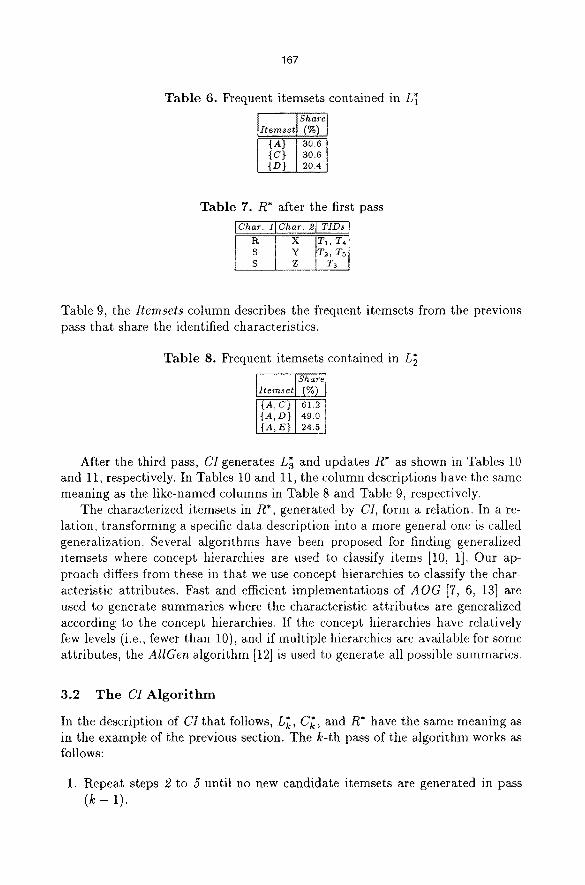
We now present an example to demonstrate the CI algorithm and describe the primary data structures. In this example, let L~ and C~ denote the set of frequent itemsets from pass k and the set of candidate itemsets from pass k, respectively, and let R* denote the relation containing the characterized itemsets. Each ele- ment of L~ and C~ contains three attributes: the itemset, the total item count local share, and the total item amount local share. Each element of R* contains one attribute for each characteristic of interest and an attribute containing a list of all frequent itemsets sharing the corresponding characteristic attributes. Assume we are given the transaction database shown in Table 5. Also assume the user-specified minimum share is 15%. In Table 5, the column descriptions have the same meaning as the like-named columns in Table 1. Our task is to trace through the first three passes of CI to generate and store the characterized itemsets in R*. For this example, we consider only the total item count local share to determine whether an itemset is frequent.
Table 5. A smaller example transaction database with counts ITIDIA ]BI CIDIE]
After the first pass, CI generates L~ and R* as shown in Tables 6 and 7, respectively. In Table 6, the Itemset column describes the items in each itemset and the Share column describes the total item count local share. In Table 7, the Char. 1 and Char. 2 columns describe the characteristics retrieved from the external database(s), and the TIDs column describes the transactions that share the corresponding characteristics (the TIDs are not actually stored in R* and are merely shown here for reader convenience). The domain of the first and second characteristic is {R, S} and {X, Y, Z}, respectively.
After the second pass, CI generates L~ and updates R* as shown in Tables 8 and 9, respectively. In Tables 8 and 9, the column descriptions have the same meaning as the like-named columns in Table 6 and Table 7, respectively. Also in
167
Table 6. Frequent itemsets contained in L~ Share
Itemset (%)
{c } 30.6 {D] 20.4
Table 7. R* after the first pass IChar. llChar. 21 TIDs I
S Y T~, T5 S Z '/'3
Table 9, the Itemsets column describes the frequent itemsets from the previous pass that share the identified characteristics.
Table 8. Frequent itemsets contained in L~ Share
Itemset (%) {A'C}t 61~2 [ {A, D} 49.0 {A, E} 24.5
After the third pass, CI generates L~ and updates R* as shown in Tables 10 and 11, respectively. In Tables 10 and 11, the column descriptions have the same meaning as the like-named columns in Table 8 and Table 9, respectively.
The characterized itemsets in R*, generated by CI, form a relation. In a re- lation, transforming a specific data description into a more general one is called generalization. Several algorithms have been proposed for finding generalized itemsets where concept hierarchies are used to classify items [10, 1]. Our ap- proach differs from these in that we use concept hierarchies to classify the char- acteristic attributes. Fast and efficient implementations of AOG [7, 6, 13] are used to generate summaries where the characteristic attributes are generalized according to the concept hierarchies. If the concept hierarchies have relatively few levels (i.e., fewer than 10), and if multiple hierarchies are available for some attributes, the AllGen algorithm [12] is used to generate all possible summaries.
3.2 T h e CI A l g o r i t h m
In the description of CI that follows, L~, C~, and R* have the same meaning as in the example of the previous section. The k-th pass of the Mgorithm works as follows:
1. Repeat steps 2 to 5 until no new candidate itemsets are generated in pass ( k - 1).
168
Table 9. R* after the second pass [Char. ifChar. 2[ TIDs [Itemsets t R I X T1, T" ({A},6),({C},9),({D}, 2') S Y Tu, T~ ({A}, 6), ({C},4), ({D}, 7)
S Z T3 ({A],3), ({C],2), ({D], 1)
Table 10. Frequent itemsets contained in L~ Share
Iternset (%) {A,C,D} 69.4 ] {A,C ,E} 34.7
2. Generate the candidate k-itemsets in C~ from the frequent (k - 1)-itemsets in L~_ 1 using the Aprwri method described in [2, 5].
3. Partition the frequent (k - 1)-itemsets in L~_ 1 and update the candidate itemsets in C;,. a. Repeat steps 3-b to 3-funtil there are no more transactions to be retrieved
from the database. b. Retrieve the next transaction from the database. c. Retrieve the corresponding characteristic tuple from R*. d. For each (k - 1)-itemset in the transaction, if it is contained in L~_I,
update the characteristic tuple. (i) If itemset summary attributes already exist for this (k - 1)-itemset
in the characteristic tuple, go to step 3-d-ii. step. Otherwise, create new itemset summary attributes in the characteristic tuple.
(ii) Increment the total quantity and total value attributes for this ( k - 1)-itemset in the characteristic tuple.
e. If the characteristic tuple has been updated, save it in R*. f. For each k-itemset in the transaction, if it is contained in C~, increment
the associated total quantity and total value attributes. 4. Save the frequent k-itemsets in L~,.
a. Repeat steps ~-b and 4-c until there are no more itemset tuples in C~. b. Retrieve the next itemset tuple from C~. c. If the share of this itemset tuple is greater than the minimum specified,
copy the itemset tuple to L~. 5. Delete C~. 6. Save R*.
The first pass of the algorithm is a special pass which generates the frequent 1-itemsets and the characteristic relation, as follows:
1. Generate the candidate 1-itemsets in C~ and the characteristic relation R*. a. Repeat steps 1-b to l - f until there are no more transactions to be retrieved
from the database. b. Retrieve the next transaction from the database.
169
T a b l e 11. R* after the third pass IChar. lIChar. 21TIDs IItemsets } [ R 1 X T'l,'T.({A},6),({C},9),({D},2),({A,C},I5),({A,D),r),({A,E},6) [
S Y T2, Tsl({A},6), ({C},4), ({D}, 7), ({A,C}, 10), {{A,D),t3), ({A,E),6)[ S z ,1 Ta, ,l({a},3), ({c},2), ({D}, 1), {,IA, C},5), ({A,D},4) [
c. For each 1-itemset in the transaction, if an itemset tuple already exists in C[, go step 1-d. Otherwise, create a new itemset tuple in C~.
d. For each 1-itemset in the transaction, increment the total quantity and total value attributes of the associated itemset tuple in C~'.
e. Using the appropriate key(s), retrieve the characterizing attributes for this transaction from the external database(s).
f. If a characteristic tuple containing these characteristics already exists in R*, go step 1-b. Otherwise, create a new characteristic tuple in R*.
2. Save the frequent 1-itemsets in L~. a. Repeat steps 2-b and 2-c until there are no more itemset tuples in C~'. b. Retrieve the next itemset tuple from Ci*. e. If the share of this itemset tuple is greater than the minimum specified,
copy the itemset tuple to L~. 3. Delete C['. 4. Save R*.
The running time and space requirements of CI are O(H , It]) and O(Is[), respectively, where ]c I is the number of candidate itemsets in all iterations of the algorithm, Iq is the number of transactions, and Isl is the size of the largest candidate itemset in any pass.
4 E x p e r i m e n t a l R e s u l t s
We ran all of our experiments on an IBM AT-compatible personal computer, consisting of a Pentium P166 processor with 64 MB of memory running Win- dows NT Workstation version 4.0. Input data was from a large database supplied by a commercial partner in the telecommunications industry. The database con- tained approximately 3.3 million tuples representing account activity for over 500 thousand customer accounts and 2200 unique items (identified by integers in the range [1. . .2200]). Each tuple is either an equipment rental or service transaction containing the number of items and the cost of each item. An item- set was considered to be frequent if at least one of the following three conditions held: the minimum support was greater then 0.25%, the total item count global share was greater than 0.25%, or the total item amount global share was greater than 0.25%.
The 20 most frequent 1-itemsets ranked by support, total item count global share, and total i tem amount global share are shown in Figures 1, 2, and 3, respectively. In Figures 1 to 3, the first row of bars (i.e., those at the front of
170
the graph) corresponds to the total item amount global share (i.e., value), the second row corresponds to the total item count global share (i.e., quantity), and the third row corresponds to the support. The height of each bar corresponds to the percentage of share or support for the associated 1-itemset. There were 109 frequent l-itemsets discovered.
Figure 1 shows that support over-represents the actual frequency with which a 1-itemset is purchased, in terms of both the quantity and value of the pur- chases. The support for the most frequent 1-itemset is approximately 25%, yet this itemset represents only approximately 5% of the total quantity of items purchased and only approximately 2% of the total value of items purchased. The ranking of these same l-itemsets by total item count global share is similar to that of support, but the ranking by total item amount global share shows significant variation from both support and total item count global share.
Fig. 1 .20 most frequent 1-itemsets ranked by support
Figure 2 shows that 14 of the frequent 1-itemsets that were ranked highest by support (i.e., those identified by integers less than or equal to 20), also appear in the 20 most frequent 1-itemsets ranked by total item count global share. The remaining six 1-itemsets (i.e., 101, 81, 25, 107, 100, 34) are shown to have a higher ranking when ranked by total item count global share. The 1-itemsets that include items 100, 101, and 107 are especially noteworthy since there were only 109 frequent 1-itemsets ranked. The support measure considers these items to be among the least important, yet when ranked by total item count global share, they are ranked eleventh, first, and eighth, respectively.
Figure 3 shows that nine of the frequent 1-itemsets that were ranked highest by support, also appear in the 20 most frequent 1-itemsets ranked by total item amount global share. It also shows that nine of the most frequent 1-itemsets which were ranked in the bottom 50% by support, are shown to be among the 20 most frequent when ranked by total item amount global share.
Similar results to those shown in Figures 1 to 3 were obtained when rank- ing k-itemsets. We present the results for 2-itemsets, shown in Table 12. Ta- ble 12 shows three sets of rankings for 2-itemsets, where each set contains three columns. In Table 12, the Support, Share (Quantity), and Share (Value) columns
171
...... ........................ I i l
. . . . . l i lO.QO%
S,00%
• l$1~ne~ I t o m l o l I~1 " o ~
Fig. 2. 20 most frequent 1-itemsets ranked by total item count global share
Fig. 3. 20 most frequent 1-itemsets ranked by total item amount global share
describe 10 itemsets ranked by support, total item count global share, and total item amount global share, respectively. In the first set, the first column shows the 10 most frequent 2-itemsets ranked by support. The second and third columns show the corresponding rank for these itemsets ranked by total item count and total item amount global share, respectively. In the second set, the second col- umn shows the 10 most frequent 2-itemsets ranked by total item count global share. The first and third columns show the corresponding rank for these item- sets ranked by support and total item amount global share, respectively. In the third set, the third column shows the 10 most frequent 2-itemsets ranked by total item amount global share. The first and second columns show the corre- sponding rank for these itemsets ranked by support and total item count global share. There were 351 frequent 2-itemsets.
The 2-itemset ranked as most frequent by support (refer to the first set) and total item amount global share was ranked fourth by total item count global share. While this itemset does not represent the most frequent itemset sold in terms of the quantity of items, it was purchased in the greatest number of transactions and had the highest gross income of all 2-itemsets. In contrast, the
172
Table 12.2-itemsets ranked by support and share Set i Rankings Set .~ Rank~ngs II "' Set 3 Rankings t
I I Shore I Share II I Share I Sharell ................ I Share t Sharel Support (Quantity Value) Support (Quantity) (Value) Support (Quantity) (Value)
13 2 17 3 19 4 20 5 22 6 27 7 35 8 47 190 41
2-itemset ranked tenth by support, for instance, was ranked 41-st by total item count global share and 109-th by total item amount global share. This itemset is ranked highly by support, yet its contribution to gross income is comparatively l o w .
The 2-itemset ranked as most frequent by total item count global share (refer to the second set) was ranked 306-th by support. This is an itemset where the items are typically purchased in multiples. Consequently, it is purchased more frequently than support seems to indicate. Similarly, 13 of the 15 most frequent 2-itemsets ranked highly by total item count global share are ranked below 291 by support.
The 2-itemset ranked tenth by total item amount global share (refer to the third set) was ranked 336-th by support and 350-th by total item count global share. The items in this itemset are relatively expensive items. Consequently, although not purchased as frequently as many other items, its contribution to gross income is comparatively high.
5 C o n c l u s i o n
We have introduced the share-confidence framework for knowledge discovery from databases which classifies itemsets based upon characteristic attributes ex- tracted from external databases. We suggested how characterized itemsets can be generalized according to concept hierarchies associated with the characteristic attributes. Experimental results demonstrated that the share-confidence frame- work can give more informative feedback than the support-confidence framework.
R e f e r e n c e s
1. R. Agrawal, K. Lin, H.S. Sawhney, and K. Shim. Fast similarity search in the presence of noise, scaling, and translation in time-series databases. In Proceedings of the 21th International Conference on Very Large Databases (VLDB'95), Zurich, Switzerland, September 1995.
173
2. R. Agrawal, H. Marmila, R.Srikant, H.Toivonen, a~d A.I. Verkamo. Fast discov- ery of association rules. In U.M. Fayyad, G. Piatetsky-Shapiro, P. Smyth, and R. Uthurusamy, editors, Advances in Knowledge Discovery and Data Mining, pages 307-328, Menlo Park, CA, 1996. AAAI Press/MIT Press.
3. R. Agrawal and J.C. Schafer. Parallel mining of association rules. IEEE Transac- tions on Knowledge and Data Engineering, 8(6):962-969, December 1996.
4. S. Brin, R. Motwani, and C. Silverstein. Beyond market baskets: Generalizing as- sociation rules to correlations. In Proceedings of the A CM SIGMOD International Conference on Management of Data (SIGMOD'97), pages 265-276, May 1997.
5. S. Brin, R. Motwani, J.D. Unman, and S. Tsur. Dynamic itemset counting and implication rules for market basket data. In Proceedings of the ACM SIGMOD International Conference on Management of Data (SIGMOD'97), pages 255-264, May 1997.
6. C.L. Carter and H.J. Hamilton. Efficient attribute-oriented algorithms for knowl- edge discovery from large databases. IEEE Transactions on Knowledge and Data Engineering. To appear.
7. C.L. Carter and H.J. Hamilton. Performance evaluation of attribute-oriented al- gorithms for knowledge discovery from databases. In Proceedings of the Seventh IEEE International Conference on Tools with Artificial Intelligence (ICTAI'95), pages 486-489, Washington, D.C., November 1995.
8. C.L. Carter, H.J. Hamilton, and N. Cercone. Share-based measures for itemsets. In J. Komorowski and J. Zytkow, editors, Proceedings of the First European Con- ference on the Principles of Data Mining and Knowledge Discovery (PKDD'97), pages 14-24, Trondheim, Norway, June 1997.
9. D.W. Cheung, A.W. Fu, and J. Han. Knowledge discovery in databases: a rule- based attribute-oriented approach. In Lecture Notes in Artificial Intelligence, The 8th International Symposium on Methodologies for Intelligent Systems (ISMIS'94), pages 164-173, Charlotte, North Carolina, 1994.
10. J. Han and Y. Fu. Discovery of multiple-level association rules from large databases. In Proceedings of the 1995 International Conference on Very Large Data Bases (VLDB'95), pages 420-431, September 1995.
11. J. Han and Y. Fu. Exploration of the power of attribute-oriented induction in data mining. In U.M. Fayyad, G. Piatetsky-Shapiro, P. Smyth, and R. Uthurusamy, editors, Adavances in Knowledge Discovery and Data Mining, pages 399-421. AAAI/MIT Press, 1996.
12. R.J. Hilderman, H.J. Hamilton, R.J. Kowatchuk, and N. Cercone. Parallel knowledge discovery using domain generalization graphs. In J. Komorowski and J. Zytkow, editors, Proceedings of the ~r s t European Conference on the Principles of Data Mining and Knowledge Discovery (PKDD'97), pages 25-35, Trondheim, Norway, June 1997.
13. H.-Y. Hwang and W.-C. Fu. Efficient algorithms for attribute-oriented induction. In Proceedings of the First International Conference on Knowledge Discovery and Data Mining (KDD'95), pages 168-173, Montreal, August 1995.
14. J.S. Park, M.-S. Chen, and P.S. Yu. An effective hash-based algorithm for mining association rules. Proceedings of the ACM SIGMOD International Conference on Management of Data (SIGMOD'95), pages 175-186, May 1995.