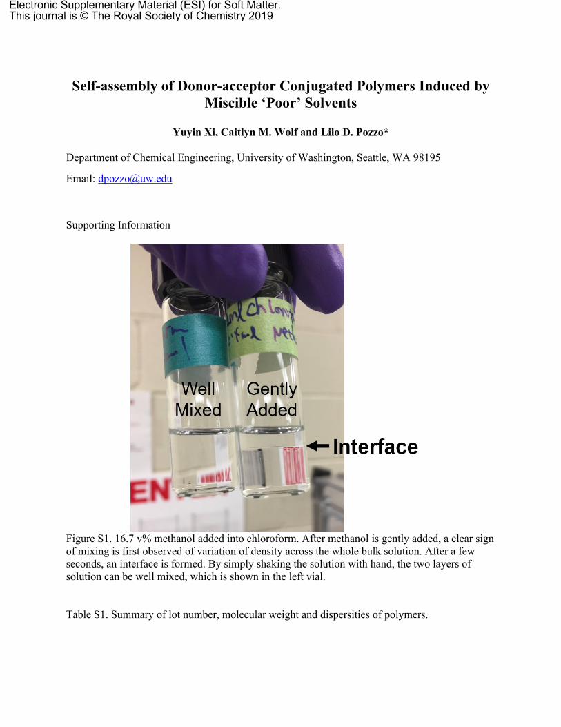
Figure S1. 16.7 v% methanol added into chloroform. After methanol is gently added, a clear sign of mixing is first observed of variation of density across the whole bulk solution. After a few seconds, an interface is formed. By simply shaking the solution with hand, the two layers of solution can be well mixed, which is shown in the left vial.
Table S1. Summary of lot number, molecular weight and dispersities of polymers.
Figure S2. AFM images of 1.6 mg/ml DPPDTT in chloroform mixed with (a) (b) (c) (d) 10 v% methanol and (e) (f) (g) (h) 20 v% methanol after aging for (a) (e) 2 hrs, (b) (f) 3 days, (c) (g) 6 days, (d) (h) 12 days.
Figure S3. The corresponding 2-D GIWAXS pattern of the samples in Figure S1 of 1.6 mg/ml DPPDTT in chloroform mixed with (a) (b) (c) (d) (e) 10 v% methanol and (f) (g) (h) (i) (j) 20 v% methanol after aging for (a) (f) 2 hrs, (b) (g) 3 days, (c) (h) 6 days, (d) (i) 12 days, (e) (j) 24 days. (k) Reduced 1-D profiles in the out-of-plane direction (φ=105˚ with 5˚ integration angle).
Figure S4 shows sTEM image and electron diffraction pattern on the nanoparticles and nanoribbons.
The formation of the nanoparticles is attributed to the Pd catalyst contaminates from the polymer
samples. The generation of Pd nanoparticles are visible under sTEM for some of our samples.
Electron diffraction on the nanoparticles spot show that the nanoparticles are very crystalline in
comparison to the nanoribbons. It is possible that the addition of methanol caused the reduction of
residual catalyst leading to the formation of Pd nanoparticles. The (110) face of Pd crystal matches
with the peak at q=2.2 Å-1 and (200) face corresponds to the peak at q=3.2 Å-1.
Although Pd nanoparticles exhibit well-defined peaks at high q-range, no evidence that palladium
particles affect or interference with the low-q scattering data (SANS and low-q GIWAXS) from
polymers was noticed. In GIWAXS data, only the high-q peaks at q=2.2 Å-1 and 3.2 Å-1 grow
with aging when methanol is added (Figure S3) and nanoparticles are formed. All the other
polymer peaks and features stay the same as a function of aging. This indicates that the
generation of Pd particles does not alter the polymer peaks. With respect to SANS experiments,
the neutron scattering contrast between the hydrogenated polymer molecules and the deuterated
chloroform is about one order of magnitude larger than that between palladium particles and the
solvent. Moreover, the much larger size of the polymer structures that are formed (i.e.
micrometers long), as compared to the Pd nanoparticles (~10 nm), leads to total dominance of
the scattering at very low angles (SANS region) by the conjugated polymer.
Figure S4 (a) sTEM image of 1.6 mg/ml DPPDTT with 20 vol% methanol. Electron diffraction patterns on (a) nanoparticles and (b) nanoribbons.
The dielectric constant measurement was achieved by using an Anton Paar MCR 301 stress
controlled rheometer. The detailed experimental set up is described in our previous publication. 1
Basically, a 25 mm parallel plate geometry was used to define a gap of 250 μm. A solvent trap
was used to prevent the solvent from evaporating. A gold wire was used to connect the upper
plate shaft and the bottom plate to a Agilent e4980 LCR meter. A frequency sweep between 20
Hz and 1 MHz with a 20 mV perturbation voltage was used to obtain the dielectric constant of
different mixtures.
20
15
10
5
'
0.80.60.40.20.0
Poor Solvent Ratio
DMSO ACN Methanol Acetone IPA Hexanes Chloroform
Figure S5. Measured dielectric constant of chloroform mixture with various poor solvents of different ratios.
Figure S6. AFM images of 1.6 mg/ml DPPDTT in chloroform mixed with 20 v% (a) DMSO (b)
Acetonitrile (ACN) (c) IPA (d) Acetone. The samples were cast after preparation without aging.
Figure S7. AFM images of films spin coated from1.6 mg/ml DPPDTT mixed with (a) 30 v% IPA, (b) 30 v% acetone and (c) 40 v% acetone. The samples are cast within a day after preparation.
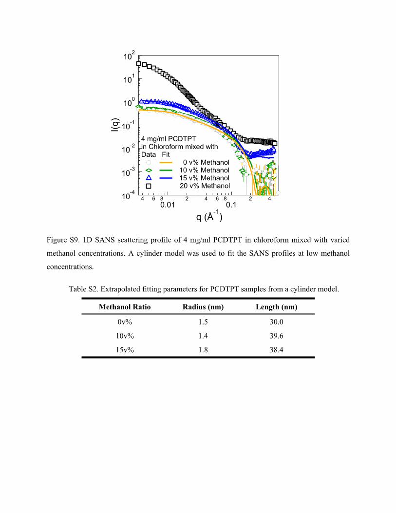
In this manuscript, two models were used to quantify polymer nano-structures and conformations.
The semi-flexible cylinder model is used to model all polymers in dissolved states. The combined
model of parallelepiped and dissolved polymers is used for systems that have also clearly started
to self-assemble into nanoribbons but still contain ‘free’ dissolved polymer in equilibrium. At low
methanol concentrations (below 15 v%), no clear sign of self-assembly into nanoribbons is
observed, so these samples are modeled with a flexible cylinder model to probe the polymer
conformation. For high methanol concentration (20 vol%) and those with DMSO and acetonitrile
that clearly form nanoribbons, a combined model (i.e. ribbons plus dissolved polymer) is used to
quantify the cross-sectional size of the ribbons and the relative amount of polymer that is found in
nanoribbons. More detailed description of each model is presented below.
Description of combined model of parallelepiped and dissolved polymers with excluded
volume effect.
Polymer nanoribbons were modeled with parallelepiped model 2,3 combined with dissolved
polymer model considering excluded volume effect 4,5. The fraction of parallelepiped model ( ) 𝜑𝑓
indicates the amount of polymers that form nanoribbons. The form factor of the combined model
Figure S8. (a) SANS profiles of DPPDTT with 20 v% and 40 v% n-Hexane. The profiles are fit with flexible cylinder model. (b) The extrapolated contour length, Kuhn Length, and radius from the model.