Missing Women and the Price of Tea in China:The Effect of Relative Female Income on Sex

Imbalance(Incomplete)

Nancy Qian∗

Department of Economics, MITCambridge, Massachusetts

October 26, 2004

Abstract

Severe sex imbalance exists in many developing countries. However,the observed association between sex ratios and economic conditions re-flects omitted variables such as sex preference. This paper uses exogenousincreases in agricultural income and relative female income caused bypost-Mao reforms to estimate the effect of total household income andrelative female income on sex ratios of surviving children. To correct formeasurement error, I instrument for tea planting with geographical data.The results show that increasing income alone has no effect whereas in-creasing relative adult female income has an immediate and positive effecton survival rates for girls and education attainment for boys and girls.Conversely, increasing relative adult male income has an immediate andnegative effect on the survival rate and education attainment for girls.(JEL I12, J13, J16, J24, O13, O15)

∗I am extremely grateful to my advisors Abhijit Banerjee, Esther Duflo and Josh Angristfor their guidance and support; Ivan Fernandez and Ashley Lester for in-depth discussions anduseful suggestions; Fred Gale at the USDA, Zhang Yaer at the China Institute for PopulationStudies, the Michigan Data Center, Huang Guofang and Terry Sicular for data assistance; andthe participants of the MIT Development Lunch, Social Science Research Council Conferencefor Development and Risk Fellowship Recipients, the Harvard East Asian Conference, andthe International Conference on Poverty, Inequality, Labour Market and Welfare Reform inChina at ANU RSSS RSPAS for their comments. I would like to acknowledge financial sup-port from the National Science Foundation Graduate Research Fellowship, the Social ScienceResearch Council Fellowship for Development and Risk, and the MIT George C. Schultz Fund.All mistakes are my own. Please send comments or suggestions to nqian@mit.edu.

1

1 Introduction

Many Asian populations are characterized by highly imbalanced sex ratios. For

example, only 48.4% of the populations of India and China are female in com-

parison with 50.1% in western Europe. Amartya Sen (1990, 1992) termed this

phenomenon "missing women". The existence of "missing women" has been

discussed in studies of India and China by Burgess and Zhuang (2001), Clark

(2000), Coale and Banister (1994), Gu and Roy (1995), Rosenzweig and Foster

(2001), Das Gupta (1987) and Jensen (mimeo). The phenomenon of "missing

women" is almost certainly due to behavioral factors that reflect a preference for

male children.1 These include selective abortion, infanticide and neglect (Foster

and Rosenzweig, 2001). The result is that an estimated 30-70 million women

are "missing" from India and China alone.

In the long run, skewed sex ratios can affect the marriage and labor markets

(Angrist, 2002). A more immediate concern is that to select the sex of the child,

parents without access to pre-natal gender revealing technologies must resort to

infanticide or other forms of neglect which ultimately lead to the death of a

child.

The purpose of this paper is to estimate the effect of economic conditions on

sex ratios. Cross-country comparison shows that income and sex imbalance are

negatively correlated. However, interpretation of this relationship is complicated

by two facts: 1) sex imbalance also exists in rich countries (South Korea and

Taiwan have the same sex ratios as China and India), and 2) sex imbalance

in China is increasing, not decreasing, with economic growth. (Chart 1 shows

that the fraction of males increased from approximately 50% for cohorts born

before 1970 to almost 54% for cohorts born in the late 1980s). An alternative

explanation posited by economists beginning with Becker argued that sex ratios

respond to sex-specific economic conditions. For example, parents may wish to

1 In a recent study of the impact of hepatitis B on sex ratios, Oster (2004) uses a back-of-the-envelope calculation to argue that 90% of the observed sex imbalance in China is explained bythe effect of hepatitis infection of pregnant mothers on miscarriage of female fetuses. However,she ignores the fact that sex imbalance in China exists only for cohorts born after 1969 and theincrease in sex imbalance was discrete (Chart 1). Since there is no evidence that hepatitis Binfection rates increased discretely during this period, it is likely that her results overestimatesthe true effect of hepatitis.

2

avoid female children when marriage requires a large dowry. The main empirical

challenge in establishing the link between sex ratios and economic conditions is

that both sex ratios and economic variables may reflect omitted variables such

as sex preferences.

The principle contribution of this paper is to develop and implement a strat-

egy that captures the causal effect of economic conditions on sex ratios in China

using exogenous variation in regional incomes over time. In particular, I exploit

the variation in intensity of adult female and male labor input across crops and

the exogenous variation in agricultural income caused by two post-Mao reforms

(1978-1980). First, I use the increase in value of tea relative to grains and the

fact that women pick tea to estimate the effect of an increase in relative fe-

male income on sex ratios. In other words, I compare the sex ratio for cohorts

born before and after the reform, between counties which plant tea and counties

which do not. Second, I use the increase in value of orchard fruits relative to

grains and the fact that in the time and regions relevant to this study, men

are the main producers of orchard fruits to repeat the experiment to estimate

the effect of an increase in relative adult male income. Third, I use cash crops

which experienced a similar value increase to tea but for which neither sex had

a comparative advantage to estimate the effect of an increase in total household

income without changing relative male and female incomes. I address the prob-

lem of measurement error in the data and the possibility that families which

cared more about girls chose to plant tea after the increase in relative prof-

itability of tea by instrumenting for tea planting with geographic data. Finally,

I repeat the experiments to estimate the effects of relative adult female income,

relative adult male income and total household income on education attainment.

Setting the study in China during the period of 1962-1990 has the advantages

that migration was strictly controlled, almost no technological change occurred

in tea production and sex-revealing technologies were unavailable to China’s

rural population for most cohorts in the study (Diao et. al., 2000; Zeng, 1993).

In addition, the One Child Policy controlled the number of children each family

was allowed to have.

The results show that economic conditions do affect the desirability of girls

3

relative to boys. An increase in relative adult female income has an immediate

and positive effect on the survival rate of girls. In the early 1980s, in rural China,

increasing female adult income by US$7.7 (10% of average rural household in-

come) increased the number of surviving girls by 1 percentage-point on average.

Increasing relative female income also increased education attainment for girls.

Conversely, increasing relative adult male income decreased both survival rate

and education attainment for girls. Increasing total household income without

changing the relative incomes of men and women had no effect on survival rates

and education attainment of girls. These results are consistent with the obser-

vation that sex-imbalance exists in rich counties as well as poor countries and

does not always decrease as countries become richer.

In addition to being of general scientific interest, the results of my study point

to the possibility of non-coercive policies that can affect sex ratios. In particular,

the results presented here suggest that factors that increase the economic value

of women will also increase the probability that female infants are carried to

term and female children live to adulthood.

Section 2 describes the background. Section 3 presents a simple model of the

effect of adult income on sex imbalance. Section 4 describes the data. Section

5 discusses the empirical strategy and results. Section 6 offers conclusions.

2 Background

2.1 Previous Works

Becker (1981) argued that sex preference is not only affected by slow-moving

endemic "cultural" features of society. Many studies since then have shown

that it is often correlated with household income. However, the nature of this

relationship is anything but settled. Edlund (1999) suggests that poorer states

in India have more girls and rich states have more boys. For China, Gu and

Roy (1995) show that the poorest regions, along with the richest regions have

the least sex imbalance. Burgess and Zhuang (2001) use micro-level data from

two provinces to show that boy-preference in allocation of health goods and

tertiary education investment occur more in poor households. And surprisingly,

4

Li (2002) found no correlation between sex ratios and factors such as household

income, parents’ education and the amount of monetary fine associated with

the One Child Policy in a study using household level data from 8 provinces for

children born during 1982-1987.

A second branch of the household literature, beginning with Ben Porath’s

study of Israeli female labor supply (1978, 1979), has also argued that relative fe-

male income and/or education also affect sex preference. For India, Rosenzweig

and Shultz (1982) showed that female children receive a larger share of house-

hold resources relative to male children in communities where women’s expected

labor market employment is relatively high. In order to establish a causal rela-

tionship between parental outcome and child outcome, Foster and Rosenzweig

(2001) uses the practice of patrilocal exogamy and productivity changes caused

by technology adoption during the Green revolution to exploit the variation in

returns to male and female children to identify how survival rates respond to

economic incentives. Increased wages and/or education for adult women have

also been shown to have a positive correlation with health and education out-

comes for girls by Duflo (2002) in South Africa; Clark (2000), and Das Gupta

(1987) in India; and Thomas et. al. (1991) in Brazil. For China, Burgess and

Zhuang (2001) show that boy-preference is stronger in areas which have fewer

non-farm employment opportunities. If men are more valuable for farm labor,

the results suggest that increasing employment opportunities for women would

decrease boy-preference. However, they do not establish this link directly.

2.2 Agricultural Reforms

Pre-1978 Chinese agriculture was mainly characterized by intense focus on grain

production, allocative inefficiency, lack of incentives for farmers and low rural

incomes (Sicular, 1988; Lin, 1988). Agricultural policies aimed at subsidiz-

ing urban industrial populations with cheap food mainly centered around pro-

duction planning. After 1953 (tong gou tong xiao), planning was done at the

central level, adjusted through discussion with the other levels of government,

re-approved by the central government, and finally sent to production brigades

and teams (Sicular, 1988a). Planning included mandatory targets for crop culti-

5

vation, areas sown, levels of input applications and planting techniques by crop.

Amongst these targets, sown area was the most important, in part because these

were easier to enforce. Mandatory targets required for grain cultivation often

resulted in lower production of other crops that could have been more profitable

in forest, grassland, or hilly areas.

Crops were divided into three categories. Category 1 included crops neces-

sary for national welfare: grains, all oil crops and cotton. Procurement prices

for grain during this period were generally 20%-30% lower than market prices

(Perkins, 1966). Market trade of these products was strictly prohibited (Sicluar,

1988a). Category 2 included up to 39 products, including: livestock, eggs, fish,

hemp, silkworm cocoons, sugar crops, medicinal herbs and tea (Sicular, 1988b).2

Category 3 included all other agricultural items, mostly minor local items. These

were not under quota or procurement price regulation.

Under the unified system, the central government set procurement quotas

for crops of the categories 1 and 2 which filtered down to the farm or collective

level. Quota production was purchased by the state at very low prices. These

quotas were set so that farmers retained enough food to meet their own needs

but in reality, farmers were left with little remaining surplus (Perkins, 1966).

Non-grain producers produced grain and staples for their own consumption and

sold all the cash crop output to the state at suppressed prices. Under this

system, farmers had very little incentive to produce more than their quota.

After the Great Famine (1959-1961), the government re-emphasized grain

production by increasing procurement prices for grain relative to other crops.

Charts 2A and 2B show that procurement prices froze during the Cultural Rev-

olution. The state resorted to commercial and production planning to carry out

the objectives of grain production (yi liang wei gang) and self-sufficiency (zi li

geng sheng). Increased production was promoted by enforcing mandatory sown

area targets for crops and self-sufficiency by purchasing but not selling grain

and oils in rural areas. Mandatory sown area targets often required cultivation

on land unsuitable for grain. Grain production grew at substantial cost of other

production. Production of crops which competed with grain for land suffered.

2The number of crops in each category changed over time. And the number of cropsreported in for each category for a given year may vary across sources.

6

Living standards declined significantly in areas suitable for commercial crops

(Lardy, 1983).

Post-Mao era reforms focused on increasing rural income, increasing deliv-

eries of farm products to the state, and diversifying the composition of agricul-

tural production by adjusting relative prices and profitability. This was mainly

carried out by two sets of policies. The first set of policies gradually reduced

planning targets and reverted to earlier policies of using procurement price as an

instrument for controlling production (Sicular, 1988a). In 1978 and 1979, quota

and above quota prices were increased by approximate 20%-30% for grain and

certain cash crops. By 1980, prices had increased across all crops. Although

category 1 crops benefited from the price increases, emphasis was placed on

cash crops from category 2. The second set of policies, called the Household

Production Responsibility System (HPRS) devolved responsibility from the col-

lective, work brigade, or work team to households (Johnson, 1996; Lin, 1988).

The HPRS was first enacted in 1980 and spread through rural China through

the early 1980s. This devolved all production decisions and quota responsi-

bilities from the work unit to individual households. Effectively, the HPRS

allowed households to take full advantage of the increase in procurement prices

by partially shifting production away from grain to cash crops when profitable.

The two reforms combined contributed to diversification of agricultural pro-

duction, greater regional specialization, and less intensive grain cultivation (Sicluar,

1988a). There was an immediate and significant increase in the output of eco-

nomic crops (Johnson, 1996; Sicular 1988a). However, although the value of all

crops increased, continued emphasis on rural-urban subsidization of grain and

other category 1 products caused the relative value of category 1 products to

decrease.3 I will compute the income from each crop directly in the next section.

But the relatively larger increase in value of category 2 crops is also reflected in

the disproportionate growth in output of category 2 crops in comparison with

category 1 crops. Charts 2A and 2B show that although output for category 1

crops increased, there is little change in the rate of increase. Chart 2C shows

the increase in the rate of increase for category 2 crops after the reform.

3The central government complained that the targets were under-fulfilled while productionof economic crops greatly exceed plans (Sicular, 1988a).

7

In a second round of reforms, in order to reduce the fiscal burden of grain

subsidies and because of excess supplies from previous years, the state increased

urban grain retail prices and stopped guarantees of unlimited procurement of

category one products at favorable prices. On average, contract procurement

prices for grain were 35% lower than market prices (Sicular, 1988a). This

combined with the de-regulation of other crops further decreased the relative-

profitability of category 1 products. This reduction in relative returns for farm-

ers was exacerbated by the uncertainty they faced from the newly opened and

yet underdeveloped market channels.

Complete substitution away from producing grains was prevented by the

state’s continued enforcement of grain production quotas and suppression of

intra-rural grain trade. As late as 1997, virtually every agricultural household

planted staple crops (Eckaus, 1999). Using the 1997 Agricultural Census, Diao

et. al. (2000) show that on average, 80% of sown area is devoted to grain and

that self-sufficiency in grain was still an important part of Chinese agriculture.

One possible cause of the magnitude and speed of the response of the Chinese

agricultural sector is the low labor productivity in the agricultural sector result-

ing from migration and other labor controls. Diao et. al. (2000) calculated that

for a household with 0.7 hectares of land, only 29% of the household’s laborers

need to work full time on agriculture to produce the same output with the same

technology. The remaining members could easily respond to take advantage of

new economic opportunities. The existence of surplus labor is consistent with

the fact that agricultural households very rarely hired labor from outside the

family. In the 1997, household on average hired 0.013 permanent and 0.004

temporary workers (Diao et. al., 2000). Plentiful cheap adult labor would also

reduce demand for child labor.

2.3 Tea and Orchard Production

This section discusses the male and female labor intensity in tea and orchard

production and how the production of each reacted to post-Mao reforms. I will

also directly estimate the income from each crop and show that: 1) income from

category 2 cash crops (including tea and orchards) was larger than income from

8

category 1 staple crops; and 2) income from tea did not exceed income from

other category 2 cash crops. The latter fact is important in interpreting the

effect of tea as a relative female income effect and not a total household income

effect in the case where the income effect on sex ratio is non-linear. An increase

in income from tea translates into an increase in income in total household

income as well as an increase in relative female income. If the income effect on

sex ratio is linear, I can show that there is no total household income effect by

showing that cash crops in general do not have an effect on sex ratios. However,

if income effects on sex ratio is non-linear, that is, if there exists some threshold

income which must be met before income will affect sex ratio, then the logic

above is only true if income from tea does not exceed income from other cash

crops.

According to agriculture specialists and anecdotal evidence, tea is mainly

picked by women and orchard fruits, in southern China, are mainly produced

by men. Labor input data by sex by crop is not available to help determine the

cause of such sex specialization across crops. One possible explanation comes

from the combination of physical comparative advantage in the production of

each crop and the continued government restrictions which meant that every

household had to plant grain (Diao et. al., 2000; Eckaus, 1996). In other words,

women are better at picking tea than planting grain.4 In households that wished

to produce tea after the reform, men continued to produce grain while women

switched to tea production. Consequently, an increase in the value of tea picking

translates into an increase in the value of adult female labor. Conversely, men

are better at producing orchard fruits than in producing grain.5 In households

that wished to produce orchard fruits after the reform, men switched to orchard

4Adult women have a comparative advantage to picking tea over adult men and childrenbecause tea picking favors small and agile fingers. Green tea leaves cannot be broken andsmall tender leaves are more valuable. In addition, tea bushes are on average 2.5 feet (0.76meters) tall, which disadvantages adult males who are on average taller than adult women.

5Adult men have a comparative advantage in orchard production during both sowing andpicking periods. Sowing orchard trees is strength intensive as it requires digging holes ap-proximately 3 feet (0.91 meters) deep. The strength requirement is re-enforced by the factthat Chinese soil is composed of 85% rock. The height of orchard trees means that adultmales also have an advantage in picking over adult females and children. For example, theheight of apple trees and orange trees range between 16-40 feet (4.9- 12.2meters) and 20-30feet (6.1-9.1 meters), respectively. Thus, an increase in the value of orchard fruits translatesinto an increase in the value of adult male labor.

9

production while women continued planting grains. Thus, an increase in the

value of orchard fruits translates into an increase in the value of adult male

labor.

Child labor cannot be ruled out in any agricultural production. However,

adult labor surplus resulting from land shortage, labor market and product

market controls leaves little demand for child labor. Later in this paper, I will

establish that the identification strategy does not depend on the assumptions

that only women pick tea or only men produce orchard fruits.

The main effect of post-Mao reforms for tea production was to increase pick-

ing, which translates to an increase in relative adult female income as well as an

increase in total household income and potential earning for girls. Considered

a priority crop, tea production was collectivized into 500 state tea farms in the

1950s. Procurement and retail were completely nationalized by 1958 (Ether-

ington and Forster, 1992). During the Cultural Revolution, the government

pursued an aggressive expansion of tea fields. However, since farmers had little

incentive to produce and tea picking is more difficult to enforce than sowing,

most of the sown fields were left wild and untended until the post-Mao era,

when the HPRS disaggregated the 500 state tea farms into over 90,000 house-

hold level tea production units. Tea bushes were restored by extensive tending

and pruning (Forster and Etherington, 1992). Procurement price for tea, which

was largely unchanged between 1958-1978, doubled between 1979 and 1984.

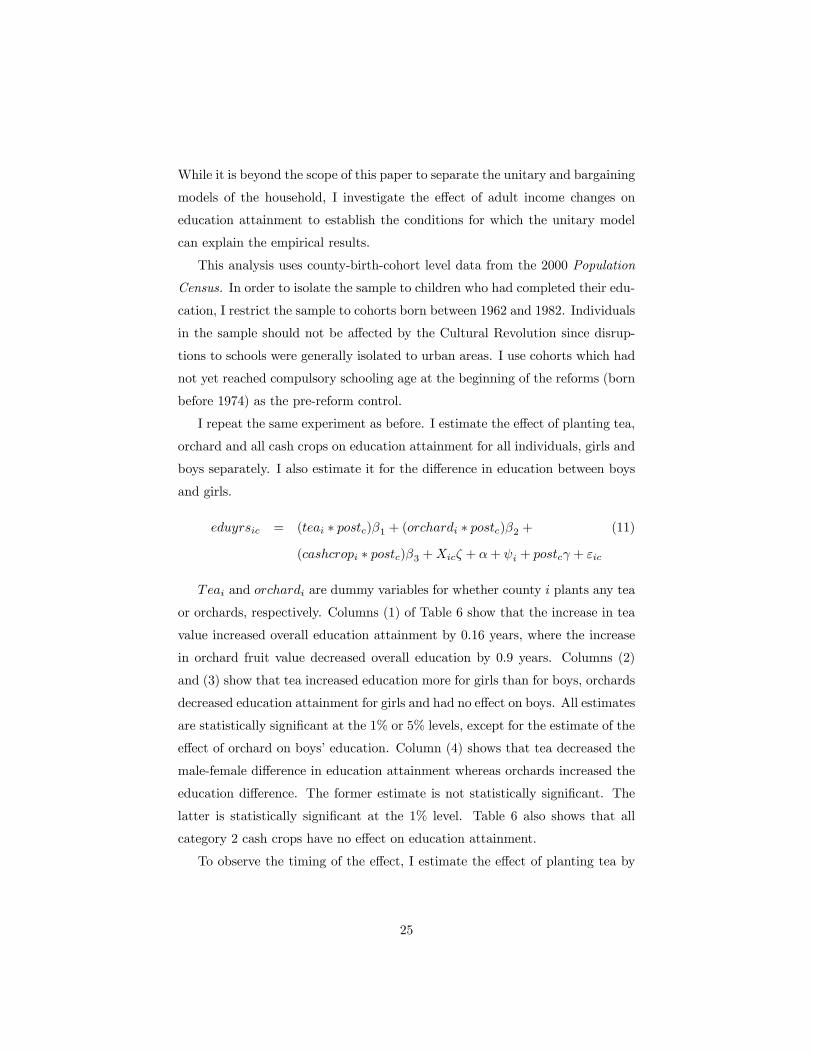
Chart 3A shows the increase in procurement price and yield for tea. Since there

was no change in sown area during this period, the yield increase reflects an

increase in picking, which, in turn, reflects an increase in the value of female

labor.

Chart 3B shows the income from grain and income from tea calculated using

procurement price data and data on the output per standard day of labor by

year and by crop. After 1979, income from tea increased at a faster rate than

income from grains. I will exploit this increase to estimate the effect of an

increase in relative adult female income on sex ratios.

Chart 4A shows the increase in orchard fruit production and procurement

price after the reform. Chart 4B shows that the calculated income from orchard

10

production increased at a faster rate than income from grains. I will exploit

this increase to estimate the effect of an increase in relative male income on sex

ratios.

Amongst category 2 crops, the government maintained more control on tea

than other crops. Unlike other category 2 crops, tea was viewed as a politi-

cal symbol by the central government from the early 1950s. In 1984, tea was

one of the 9 crops to remain under designated procurement price. The central

government continued to maintain a retail monopoly on tea up to the early

1990s. Until the late 1980s, China exported tea at subsidized prices. Part of

the subsidy was achieved by suppressing procurement prices of tea (Etherington

and Forster, 1992). Consequently, although price for tea grew significantly after

1979, tea was not as profitable as other cash crops. Chart 5 shows that the

income from tea experienced similar increases to other category 2 cash crops

immediately after the reform. But by 1983, although the income from tea con-

tinued to increase, the rate of increase was less than income from other category

2 crops. I will exploit the income increase from all category 2 crops (including

tea and orchards) to estimate the effect of an increase in total household income

on sex ratios.

3 Model of Sex Imbalance

In this section, I present a simple model of the household to illustrate the dif-

ferent mechanisms by which changes in adult income can affect sex ratios in the

observed population. The model shows that adult income affects the desirabil-

ity of daughters relative to sons through two mechanisms: 1) by changing the

consumption value of having a girl relative to having a boy; and 2) by chang-

ing the investment value of having a girl relative to having a boy. Moreover,

it shows that if households are not unitary (e.g. parents do not have identical

preferences), a change in adult income will also affect the relative desirability

of girls by changing the bargaining power of each parent within the household.

It is beyond the scope of this paper to discern whether households in rural

China are unitary. However, the model generates empirically testable predic-

tions for the case where households are unitary and parents view children only

11

as consumption goods.

3.1 Decision Rule

For most cohorts in this study, family size was constrained by China’s family

planning policies. Thus, I make the simplifying assumption that all households

have exactly one child. The only decision which faces parents is the sex of their

child. Because parents do not have access to prenatal sex revealing technology,

parents select the sex of their child by deciding to keep or kill a child once

she/he is born. Parents for each household i compare the maximum utility that

they can derive from a girl and the maximum utility they can derive from a

boy, and will choose to have a girl if V Hg − V H

b > εi, where V Hs is the indirect

utility of household H if it has a child of sex s, s ∈ {g, b}. εi is an independentand identically distributed preference shock that is normally distributed in the

population, εi v N(0, 1).

The probability of having a girl can be written as:

Pr(S = g) = Pr¡εi < V H

g − V Hb

¢= Φ(V H

g − V Hb ) (1)

An increase in the probability of having a girl will be reflected in the popu-

lation as an increase in the fraction of girls.

Let yρ, ρ ∈ {m, f} denote parents’ (mother’s and father’s) incomes. Theeffect of an increase in a parent’s income on the probability of having a girl

relative to having a boy is represented by the partial derivative of the decision

rule with respect to the parent’s income.

∂Φ

∂yρ≡ Φyρ

Note that the sign of Φyρ is determined by the sign of the derivative of the

difference between the household’s indirect utility if it has a girl and if it has a

boy with that parent’s income.

Φyρ > 0 if∂(V H

g − V Hb )

∂yρ> 0

Henceforth, denote Γyp =∂(V H

g −V Hb )

∂yρ.

12

3.2 Household Utility

uHs = uH(c), where c is the parents’ consumption bundle, is the utility function

of household H when it has a child of sex s, s ∈ {g, b}. Parents maximizeutility subject to the household budget constraint. Credit markets are assumed

to be perfect such that parents may save or borrow against the child’s adult

income. Thus, I can model parents’ consumption and investment decisions in a

one period model.

Normalize the price of consumption to equal 1. Households maximize the

weighted sum of the mother’s and father’s utilities, ums , ufs . Let y be the total

household income. The indirect utility function Vs(y) is the maximand of the

optimization above.

V Hs = max

cµums (c) + (1− µ)ufs (c), s.t. c = y

The weight, µ, which characterizes bargaining power, is a function of the

mother’s and father’s income ratio. Hence, the mother’s bargaining power is

increasing in her income and decreasing in the father’s income. Note that the

unitary model is simply the special case of the bargaining model where µ is 0

or 1.

The household budget constraint is composed of the incomes of the father,

yf , mother, ym, and a child of sex s, ys. Assume that the productivity of a child

is positively correlated with the productivity of parents such that income of a

child is a function of his/her parents’ incomes, ys = ys(yf , ym). Furthermore,

assume that the correlation is stronger between a child and a parent of the same

sex.∂yg∂ym

>∂yg∂yf

,∂yb∂yf

>∂yb∂ym

The investment value of a child is characterized by the inclusion of his/her

income in the budget constraint. Thus, the Lagrangian for the household utility

maximization is

Ls = maxc

µums (c) + (1− µ)uf (c)− λs [c− (yf + ym + ys)] ,

The effect of a parent’s income on the probability of having a girl is

Γyρ =∂µ

∂yρ

h¡umg − umb

¢−³ufg − ufb

´i+

∙λg

µ1 +

∂yg∂yρ

¶− λb

µ1 +

∂yb∂yρ

¶¸(2)

13

It follows from the first order conditions that λg and λb are the marginal

utilities of income in the two states of the world (e.g. when a household has a girl

or when a household has a boy), ∂ug∂y ,

∂ub∂y . The latter bracketed terms imply

that holding other variables constant, the effect of a parent’s income on the

probability of having a girl is increasing in the difference between the marginal

utilities of income when a household has a girl and when a household has a

boy, λg > λb. This means that if a daughter compliments income more than

a son, an increase in income will increase the desirability of daughters relative

to the desirability of sons. In other words, an increase in parents’ income will

increase the probability of having a girl if girls are luxury goods relative to boys.

Henceforth, I call this the relative "consumption value" from having girls.

Parental income also affects the probability of having a girl by changing the

relative "investment value" from having a daughter. Equation (2) shows that

holding other variables constant, the relative desirability of a girl will increase

if the parent’s income is more correlated with a girl’s income than with a boy’s

income, ∂yg∂yρ> ∂yb

∂yρ.

The terms umg − umb and ufg − ufb are the mother’s and father’s utilities from

having a girl relative to having a boy. Equation (2) shows that as long as parents

do not have the same relative utilities from having a daughter, umg − umb 6=ufg −u

fb , an increase in parental income will also affect the probability of having

a girl by affecting each parent’s bargaining power, ∂µ∂yρ.

In short, equation (2) shows that an increase in a parent’s income will affect

the relative desirability of girls by affecting: 1) parents’ bargaining power, ∂µ∂yρ;

2) the relative consumption values of girls, λg−λb; and 3) the relative investmentvalue of girls, ∂yg∂yρ

− ∂yb∂yρ

.

It is easy to see that for the special unitary case, where µ is or 1, equation

(2) reduces to

Γyρ = λg

µ1 +

∂yg∂yρ

¶− λb

µ1 +

∂yb∂yρ

¶Where the interpretation of each term is the same as before. The only

difference here is that bargaining does not play a role.

The difference between the effects of the mother’s income and the father’s

14

income for the general case can be written as

Γym − Γyf =

µ∂µ

∂ym− ∂µ

∂yf

¶h³ufg − ufb

´−¡umg − umb

¢i(3)

+λg

µ∂yg∂ym

− ∂yg∂yf

¶− λb

µ∂yb∂ym

− ∂yb∂yf

¶> 0, since

∂µ

∂ym>

∂µ

∂yf,∂yg∂ym

>∂yg∂yf

,∂yb∂ym

<∂yb∂yf

Equation (3) shows that changes in the mother’s income and the father’s

income will have different effects on the probability of having a girl because they

affect each parent’s bargaining power differently and because the correlation

between each parent’s income and a child’s income is different for boys and

girls.

So far, I have assumed that parents view children as a form of investment

as well as a form of consumption. However, it is possible that parents view

having children only as a form of consumption. In this case, the household

budget constraint does not include the income of the child and the household

maximization problem is

Ls = maxc

µums (c) + (1− µ)uf (c)− λs [c− (yf + ym)]

The effect of parental income on the probability of a girl is then

Γyρ =∂µ

∂yρ

h¡umg − umb

¢−³ufg − ufb

´i+ λg − λb (4)

The interpretation of the individual terms is the same as for equation (2).

The difference is that the effect of the change in parental income on the child’s

income, ∂ys∂yρ, no longer plays a part in the relative desirability of the child.

In the special unitary case, where µ is 0 or 1, equation (4) reduces to

Γyρ = λg − λb

Note that the equation above implies Γym = Γyf , which means that when

households are unitary and parents view children only as form consumption,

the effect of mother’s income on the probability of having a girl should be

equivalent to the effect of father’s income. The intuition is that when households

are maximizing their utility, the marginal effect of income on consumption is

15

the same across all sources of income. Consequently, if the empirical results

show that mother’s and father’s incomes have different effects on population

sex ratios, the hypothesis that parents in unitary households view children only

as a form of consumption can be rejected.

4 The Data

This paper matches the 1% Sample of the 1997 Chinese Agricultural Census,

0.1% samples the 1990 and 2000 Chinese Population Censuses, and GIS geogra-

phy data from the Michigan China Data Center at the county level. The sample

includes 1,621 counties in China’s 15 southern provinces, south of the Yellow

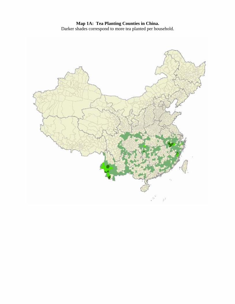
River (Huang He) where any tea is planted.6 Map 1A show that these counties

are dispersed throughout southern China. The 1990 census data contain 52

variables, amongst which are data on sex, year of birth, education attainment,

sector and type of occupation, and relationship to the head of household. Be-

cause of the different family planning policies and market reforms experienced

by urban areas and rural areas, I limit the analysis to rural households. The

individual and household level data are aggregated to the county level to match

the agricultural census data. The number of individuals in each county-birth

year cell is retained so that the later analysis are all population weighted.

Reliable data for procurement prices and output are not available for this

period at the county level. For the sake of scope, accuracy and consistency

between areas, this study uses county level agricultural data on the sown area

from the 1% sample of the 1997 China Agricultural Census. Agricultural land is

allocated by the village to farmers based on the number of members per house-

hold and quality of land. Land is usually allocated for 15 year terms (Burgess,

2004). There is no market for buying or selling land. The measurement error

bias that results from using 1997 agricultural data to predict for agricultural

conditions in the early 1980s is resolved by the instrumental variables strategy

discussed later in the paper.

To assess whether counties that do not plant tea are good control groups for

6Jiangsu, Zhejiang, Anhui, Fujian, Jiangxi, Shandong, Henan, Hunan, Hubei, Guandong,Guangxi, Sichuan, Guizhou, and Shanxi.

16

counties that plant tea, I look for systematic differences between the treatment

and control groups. The ideal control group would be identical to the treat-

ment group in every characteristic other than tea planting and the outcomes of

interest. Panel A in Table 1 show that demographic composition and educa-

tion attainment in tea counties are very similar to counties with no tea. The

difference in ethnic composition will be controlled for in the regression analysis.

Panel B shows that tea and non-tea counties are almost identical in sector of

employment. 94% of the population is involved in agriculture. Panel C shows

that households in tea counties farm less total land on average, devote more

land to rice, garden production, and less land to orchards and grass for grazing.

Tea counties also produce slightly more fish.

It is important to note the scarcity of land in the Chinese country side. On

average, agricultural households only have 4.06-4.85 mu (0.20-0.32 hectares) of

land per household. On average, households in counties that plant tea have

only 0.15 mu (0.02 hectares) of land for tea. For a visual representation of the

similarity in agricultural production between tea producing counties and non-tea

producing counties, refer the Map 1B-1E, which map agricultural production

of different types of cash crops and agricultural density. The black colored

counties are counties which produce some tea. The gray shaded counties are

counties which produce some garden vegetables (Map1B), orchard fruits (Map

1C) and fish (Map 1D). Map 1E shows counties which produce some tea and

counties where the average farmable land per household exceeds the median

of 4 mu (0.27 hectares). The maps show that tea producing counties are not

geographically distant from counties which produce other cash crops. In fact,

most tea producing counties also engage in other cash crop production.

5 Empirical Strategy

5.1 Identification

The main problem in identifying the effect of increased relative female-to-male

earnings on child outcomes is that sex selection or investment in children’s edu-

cation and relative earnings are likely to be jointly driven by omitted household

17

and community characteristics such as sex-preferences. For example, in com-

munities with no boy bias, adult women will earn more and parents will view

female children as less undesirable. When compared with communities with

strong boy-bias, where adult women earn less and parents have very strong

boy-preferences, we will find a positive correlation between adult female income

and girl survival rates. However since female earnings and girl survival rates are

jointly determined by sex preference, the correlation cannot reveal whether the

increase in girl survival rate is caused by higher female earnings or by under-

lying sex preference which drives both adult female earnings and girls’ survival

rates. This problem is addressed by exploiting the increase in relative value of

tea caused by two post-Mao policies during 1978-1980. The exogenous variation

in relative adult female earnings allows me to estimate the causal effect of an

increase in relative adult female earnings on relative survival rates of girls.

First, I estimate the effect of the agricultural reforms on girl survival rates

in tea planting regions. The identification strategy uses the fact that the rise in

adult female income varied across region and time of birth. Substantial variation

in amount of tea sown existed across regions. Therefore, the number of surviving

female children should have increased in tea planting regions for cohorts born

close to and/or after the reform, and the increase should have been larger for

regions which planted more tea. I use a differences-in-differences estimator

to control for systematic differences both across regions and across cohorts.

Only the combination of these two variations is treated as exogenous. In other

words, I compare relative survival rates between counties which plant tea and

counties which do not plant tea, for cohorts born before and after the reform.

Comparing sex ratios within counties for cohorts born before and after the

reform differences out time-invariant community characteristics. Comparing tea

planting communities to non-tea planting communities differences out changes

that are not due to planting tea. Thus, the causal effect of planting tea can be

identified as long as tea planting areas did not experience changes which were

systematically different from non-tea planting areas.

The date of birth and whether an individual is born in a tea planting region

jointly determine whether he/she was exposed to the relative adult female in-

18

come shock. In other words, tea is a proxy for female earnings. The validity

of the identification strategy does not rely on the assumption that only women

pick tea. If men or children picked tea, the proxy for relative female income will

exceed actual relative female income. Hence, the strategy will underestimate

the true effect of relative female income on sex ratio. If there are any unob-

served time-invariant cultural reasons that affect both women to pick tea and

desirability of female children, the effect will be differenced out by comparing

cohorts born before and after the reform. The identification strategy is only

in question if there is some time varying difference which coincides with the

reform. For example, if the attitudes which drive sex preference changes in tea

planting counties at the time of the reform, the estimate of the effect of plant-

ing tea will capture both the relative female income effect and the effect of the

attitude change. Or, if the reason for women to pick tea was changed by the

HPRS, the pre-reform cohort will be an inadequate control group. While I can

not resolve the former problem, I address the latter concern by instrumenting

for tea planting with time invariant geographic data.

Second, I investigate whether the increase in tea value affects relative survival

rates because of the increase in relative female income rather than an increase

in total household income. I estimate the effect of the reform on girls’ survival

in regions which plant cash crops that experienced equal or more value increase

but for which adult female labor have no comparative advantage. Third, I use

the increase in value of orchard fruits relative to other crops to investigate the

effect of an increase in relative male income on sex ratios. The identification

strategy of using exogenous price changes in sex-specific agricultural products

to identify effects of changes in female-to-male wage ratio is similar to Shultz’s

(1985) study on Swedish fertility rates in the late 19th century, where he used

changing world grain prices to instrument for changes in the female-to-male

wage ratio.

I can check the identification strategy by estimating the effect of category 1

and category 3 crops on sex ratios. Category 1 crops continued to be strictly

regulated after 1979. Category 3 crops were never regulated. Hence, the reforms

of 1978-1980 did not increase the rate of increase in the value of either group of

19

crops. If the identification strategy is valid, and the changes of sex ratios is due

to the increases in relative value of category 2 crops, then the effect of category

1 crops and category 3 crops on sex ratios should not change after the reform.

Chart 6A shows that indeed the effect of category 1 and 3 crops were identical

before and after the reform.

5.2 Timing

To see that the effect of tea and orchards on sex ratios is due to the post-Mao

agricultural reforms and not due to other changes in these regions, I check that

the effect of tea and orchard on sex ratios increased in magnitude at the time

of the reform. First, I estimate the effect of tea planted for each birth cohort.

sexic = α+1990Pl=1963

(teai × dl)βl + haniφ+ γi + ψc + εic (5)

The fraction of males in county i, cohort c is a function of: the interaction

term between teai, the amount of tea planted for each county i and dl, a variable

which indicates if a cohort is born in year l; hani, control for the fraction of Han

in each county i; γi,county fixed effects; and ψc, cohort fixed effects. Including

the fraction of Han controls for differences in family planning policies which

Hans and ethnic minorities faced. The dummy variable for 1962 and all of its

interactions are dropped. βl is the effect of planting tea on the fraction of males

for cohort l. If the effect of tea on sex ratios was due to the reform, βl should be

similar between cohorts until approximately the time of the reform, after which,

it should decrease. The coefficients in the vector βl are plotted in Chart 6B.

The effect of tea on fraction of males is more negative for cohorts born after

1979. Table 2 column (1) shows that they are statistically significant after 1979.

In a similar regression, I estimate the effect of orchard planted in each county

i on the fraction of males in county i, cohort c.

sexic = α+1990Pl=1963

(orchardi × dl)γl + haniφ+ γi + ψc + εic (6)

The coefficients in vector γl are plotted in Chart 6C. The effect of planting

orchards on the fraction of males become more positive after 1979. Table 2

column (2) show that the results are statistically insignificant. Chart 6D plots

20

the coefficients from a similar regression estimating the effect of all category 2

cash crops on fraction of males. The plot shows clearly that the effect of cash

crops on sex ratio experienced no change after the reform. Table 2 column (3)

presents the estimates.

5.3 Difference-in-Differences

To compare sex ratios in counties that plant tea to counties that do not, I

estimate the following equation where the fraction of males in county i birth

cohort c is a function of the interaction term of a dummy variable for whether

a county plants tea and a dummy variable for whether a cohort is born after

the reform, controlling for the amount of orchards and all cash crops planted,

fraction of Han, county fixed effects, and a dummy variable for being born after

the reform.

sexic = α+ (teai ∗ postc)β1 + (orchardi ∗ postc)β2 (7)

+(cashcropi ∗ postc)β3 +Xicζ + ψi + postcγ + εic

All standard errors are clustered at the county level. Table 3 columns (3) and

(4) show that for cohorts born after the reform, the fraction of males decreased

by 0.7 percentage point more in tea planting counties, where as it increased by

0.9 percentage points more in orchard planting counties. Both estimates are

statistically significant at the 5% level.

5.4 OLS by Birth Cohort

To see that the timing of the effect is unchanged by including controls for or-

chards and cash crops, I estimate the following equation.

sexic =1990Pl=1963

(teai × dl)βl +1990Pl=1963

(orchardi × dl)γl + (8)

1990Pl=1963

(cashcropi × dl)ρc + ζHanic + α+ ψi + γc + εic

Table 4 shows the coefficients in the vectors βl, γl and ρl for each birth cohort

c from 1963 to 1990. 1962 is the reference year. The timing of the change in

the effects of tea and orchard is similar to the the less restricted estimates of

21

equation (5) and (6). The coefficients are plotted in Chart 7. The plotted

coefficients show clearly that after the reform, planting orchards increased the

fraction of males in surviving population, planting tea decreased the fraction of

males and all category 2 cash crops had no effect.

5.5 OLS Issues

5.5.1 Differing Trends Across Counties

The long time horizon of the study suggests that a simple fixed effects estimate

may not adequately control for different trends across counties. I address this

issue by including linear trends at the county level. Column (1) of Table 5 shows

the differences-in-differences estimate from equation (7). Column (2) shows the

estimate with the inclusion of a county-level linear trend. The point estimate is

almost identical to the less restrictive estimate of column (1) and statistically

significant at the 5% level. Thus, the OLS estimate is robust to changes across

counties over time.

5.5.2 Migration

Strict migration controls suppressed long termmigration from rural areas through-

out the period of the study. However, if migration patterns differed significantly

between tea and non-tea areas, and between orchard and non-orchard areas, the

OLS estimate could be capturing the effects of migration rather than of income

changes. Cohorts born after the reform are 11 years of age or younger in the

1990 Census. Hence, migration would bias the estimates if households with

boys are more likely to migrate out of tea areas and households with girls are

more likely to migrate out of orchard areas. Migration controls, however, made

migration of entire households impossible. Another possible cause for bias is

if amongst pre-reform cohorts, females were more likely to migrate out of tea

areas and males were more likely to migrate out of orchard areas.

To address this problem, I use equation (7) and inferred populations to

estimate the upper and lower bounds of the effect of planting tea and orchards

on sex ratios. To calculate the inferred populations, I use the fraction of urban

residents in each province that report they are not born in that city and the

22

population of the province to calculate the maximum possible number of rural-

urban migrants per province. I use population of each county to calculate the

fraction of provincial population in each county. I then add the multiple of

this fraction and the maximum number of migrants for that province back into

each county. I assume that the new additions are all born prior to the reform.

To estimate the lower bound of the effect of tea, I assume that all the new

additions to the pre-reform cohorts in tea counties are female. To estimate

the upper bound of the effect of tea, I assume that all the new additions are

male. Similarly, for the lower bound of the effect of orchard, I assume that all the

added inferred migrants in orchard counties are male. And to estimate the upper

bound, I assume that all the inferred migrants are female. The estimated bounds

are very similar to the OLS estimates on the reported population, consequently

ruling out the possibility that the results are driven by migration.

5.6 Instrumental Variables

Two problems motivate the use of instrumental variables. First, using 1997 agri-

cultural data to proxy for agricultural conditions in previous years will cause

measurement error. Second, the OLS estimate will be biased upwards if families

which innately preferred girls relative to boys switched to planting tea after the

reform. In this case, the OLS estimate will capture the innate girl-preference

of families that chose to plant tea as well as a change in the desirability of girls

caused by an increase in female earnings. I address both problems by instru-

menting for the tea planting decisions with the average slope of each county.

Tea grows only in very particular conditions: hilltops, shielded from wind

and heavy rain, warm semi-humid places. The exclusion restriction requires

that the average slope of a county does not have any direct effect on differential

investment decisions and is also not correlated with any other covariates in

equation (7). Map 2 shows the slope variation in China, where darker areas

are steeper. Map 3 overlays the map of counties which plant tea onto the slope

map. The predictive power of slope for tea planting can be seen by comparing

the tea planting counties with the steep regions in Map 2. I use the GIS data

from Map 2 to calculate the average slope for each county and estimate the

23

following first stage equation, where both the amount of tea planted and slope

is time-invariant.

teai ∗ postc = (slopei ∗ postc)λ+ (orchard ∗ postc)δ1 + (9)

(cashcrop ∗ postc)δ2 +Xicζ + α+ ψi + postcγ + εic

I use the predicted residuals to estimate the following second stage regression.

sexic = (teai ∗ postc)β + (orchard ∗ postc)δ1 (10)

+(cashcrop ∗ postc)δ2 +Xicζ + α+ ψi + postcγ + εic

Columns (3) of Table 5 shows the first stage estimate from equation (9). The

estimate is statistically significant at the 5% level. Column (4) shows the two

stage least square estimate from equation (10). The estimate is larger than the

OLS estimate and statistically significant. Column (5) shows the two stage least

squares estimate including county-level linear trends. The estimate is similar in

magnitude to the OLS estimate but no longer statistically significant.

The two stage least square point estimate is greatly reduced by including

county-level linear trends. This suggests that there are trends in hilly areas

which are not adequately controlled for by the less restrictive 2SLS estimate.

Consequently, the exclusion restriction of the instrumental variables can only be

satisfied conditional on the trends. In other words, conditional on the county-

level linear trends, the OLS estimates are not driven by the endogenous decision

to plant tea or measurement error. The similarity in magnitude between the

2SLS and OLS estimates conditional on linear trends and between the OLS

estimate conditional on the linear trends and the OLS estimate not controlling

for the trend reinforces the robustness of the OLS estimate.

5.7 Education Attainment

The main results of the effect of relative adult earnings on sex ratios rejected the

hypothesis that parents view children only as a form consumption. However,

since increasing adult agricultural earnings also increase the earnings potential

of children, the main results cannot distinguish between the unitary model where

children are a form of investment and the bargaining model of the household.

24

While it is beyond the scope of this paper to separate the unitary and bargaining

models of the household, I investigate the effect of adult income changes on

education attainment to establish the conditions for which the unitary model

can explain the empirical results.

This analysis uses county-birth-cohort level data from the 2000 Population

Census. In order to isolate the sample to children who had completed their edu-

cation, I restrict the sample to cohorts born between 1962 and 1982. Individuals

in the sample should not be affected by the Cultural Revolution since disrup-

tions to schools were generally isolated to urban areas. I use cohorts which had

not yet reached compulsory schooling age at the beginning of the reforms (born

before 1974) as the pre-reform control.

I repeat the same experiment as before. I estimate the effect of planting tea,

orchard and all cash crops on education attainment for all individuals, girls and

boys separately. I also estimate it for the difference in education between boys

and girls.

eduyrsic = (teai ∗ postc)β1 + (orchardi ∗ postc)β2 + (11)

(cashcropi ∗ postc)β3 +Xicζ + α+ ψi + postcγ + εic

Teai and orchardi are dummy variables for whether county i plants any tea

or orchards, respectively. Columns (1) of Table 6 show that the increase in tea

value increased overall education attainment by 0.16 years, where the increase

in orchard fruit value decreased overall education by 0.9 years. Columns (2)

and (3) show that tea increased education more for girls than for boys, orchards

decreased education attainment for girls and had no effect on boys. All estimates

are statistically significant at the 1% or 5% levels, except for the estimate of the

effect of orchard on boys’ education. Column (4) shows that tea decreased the

male-female difference in education attainment whereas orchards increased the

education difference. The former estimate is not statistically significant. The

latter is statistically significant at the 1% level. Table 6 also shows that all

category 2 cash crops have no effect on education attainment.

To observe the timing of the effect, I estimate the effect of planting tea by

25

birth year.

eduyrsic =1982Pl=1962

(teai × dl)βl +1982Pl=1962

(orchardi × dl)γl + (12)

1982Pl=1962

(cashcropi × dl)ρc + ζHanic + α+ ψi + γc + εic

The coefficients for each cohort l in vectors βl, δl and ρl are shown in Ap-

pendix Table A2. They are not statistically significant. I plot the 3 year moving

averages of the estimates of tea and orchards in Charts 8A-8C. Chart 8A shows

that female education attainment was similar between tea and orchard areas

until 1976, when it increased in the former and decreased in the latter. Chart

8B shows that education attainment for boys increased in both tea and orchard

areas. Chart 8C shows that the male-female gap in education attainment began

decreasing in tea areas for cohorts born 1976 and after. In orchard areas, the

male-female gap increased for those same cohorts.

The results that increasing adult female income caused girls to be relatively

more educated and that increasing adult male income caused boys to be rela-

tively more educated can be explained by the unitary model if parents interpret

the increase in adult female (male) income as an increase in girls’ (boys’) returns

to education. The finding that an increase in adult female income increased

overall education attainment while an increase in adult male income decreased

overall education attainment is more puzzling. This can only be explained by

the unitary model if an increase in female agricultural income has a different

effect on returns to education from an increase in male agricultural income. The

lack of income data prevents a direct investigation of this hypothesis.

6 Conclusion

This paper resolves the problem of joint determination in estimating the effect

of changes in adult income on survival rate of girls. I find that increasing total

household income without changing the relative incomes of men and women had

no effect on survival rates of girls or education attainment. Increasing the share

of female income had a large and immediate positive effect on the survival rates

of girls and increased education for all children. Conversely, increasing the share

26

of male income immediately decreased survival rates and education attainment

of girls. The results suggest that parents do not have identical preferences.

The empirical findings give a clear and affirmative answer to the question

of whether sex preference responds to economic incentives in the short run. In

addition, the results say that increasing total household income without chang-

ing the relative shares of female and male income will have no effect on survival

rates. Policy makers who aim to decrease sex imbalance should create policies

that increase proportional adult earnings of the deficit sex. In other words, an

effective method of immediately decreasing excess female mortality is to increase

the relative income of adult women.

27

References

[1] Angrist, Joshua and Krueger, Alan "Empirical strategies." The Handbook

of Labor Economics, Vol. III, Chapter 23, North Holland, 1999.

[2] Banister, J. China’s Changing Population, Stanford, California: Stanford

University Press, 1987.

[3] Becker, Gary A Treatise on the Family, Cambridge, Massachusetts: Har-

vard University Press, 1981.

[4] Bourguignon, Francois, Martin Browning, Pierre-Andre Chiappori and

Valerie Lechene "Incomes and Outcomes: A Structural Model of Intra-

household Allocation." Journal of Political Economy,1993.

[5] Browning, M. and Chiappori, P. A. "Efficient intra-household allocations:

A general characterization and empirical tests." Econometrica, 66(6), 1998,

pp. 1231-1278.

[6] Burgess, Robin "Mao’s legacy: Access to land and hunger in modern

China." London School of Economics Working Paper, 2004.

[7] Burgess, Robin "Modernisation and son preference." London School of Eco-

nomics Working Paper, 2001.

[8] Clark, S. "Son preference and sex composition of children: Evidence from

India," Demography, 31(1), 2000, pp. 21-32.

[9] Coale, A. J. and Banister, J. "Five decades of missing females in China."

Demography, 31(3), 1994, pp. 459-79.

[10] Croll E., D. Davin, et. al. China’s One Child Family Policy, London:

Macmillan, 1985.

[11] Das Gupta, Monica "Selective discrimination against female children in

rural Punjab, India." Population and Development Review, 13(1), 1987,

pp. 77-100.

28

[12] Duflo, Esther (2003) "Grandmothers and granddaughters: Old age pension

and intra-household allocation in South Africa." World Bank Economic

Review, 17 (1), pp. 1-25.

[13] Eckaus, Richard "Report #50: A study of the effects of natural fertility,

weather and productive inputs in Chinese agriculture." MIT Joint Program

on the Science and Policy of Global Change, 1999.

[14] Edlund, L. "Son preference, sex ratios and marriage patters." Journal of

Political Economy, 107(6), 1999, pp. 1275-1304.

[15] Foster, Andrew D. and Rosenzweig, Mark R. "Missing women, the marriage

market, and economic growth." Brown University Working Paper, 2001.

[16] Foster, Andrew D. and Rosenzweig, Mark R. "Technical change and hu-

man capital returns and investment: Evidence from the Green Revolution."

American Economic Review, 86(4), 1996, pp. 931-953.

[17] Garg, Ashish and Morduch, J. "Sibling rivalry and the gender gap: Evi-

dence from child health outcomes in Ghana." Journal of Population Eco-

nomics, 11(4), 1998, pp. 471-493.

[18] Gu, B. and Roy, K. "Sex ratios at birth in China with reference to other

areas in East Asia: What we know." Asia-pacific Population Journal, 10(3),

pp. 17-42.

[19] Jensen, Robert "Fertility preferences and female disadvantage in the de-

veloping world: Equal treatment, unequal outcomes?" Harvard Kennedy

School Working Paper, mimeo.

[20] Johnson, Gale "China’s rural and agricultural reforms: successes and fail-

ures." Chinese Economics Research Centre at the University of Adelaide,

96(12), 1996.

[21] Lardy, Nicholas R. Agriculture in China’s Modern Economic Development.

New York, New York: Cambridge University Press, 1983.

29

[22] Lin, Justin (1988) "The household responsibility system in China’s agricul-

tural reform: A theoretical and empirical study." Economic Development

and Cultural Change, Vol. 36, pp. s199-s224.

[23] Oster, Emily "Hepatitis B and the case of the Missing Women." Harvard

Working Paper, 2004.

[24] Perkins, Dwight H. Market Control and Planning in Communist China.

Cambridge, Massachusetts: Harvard University Press, 1966.

[25] Rosenzweig, Mark R. and Schultz, T. P. "Child mortality and fertility in

Colombia: Individual and community effects." Health Policy and Educa-

tion, Vol. 2, pp. 305-348.

[26] Rosenzweig, Mark. R. and Schultz, T. P. "market opportunities, genetic

endowments, and intrafamily resource distribution: Child survival in rural

India." The American Economic Review, 72(4), 1982, pp. 803-815.

[27] Schultz, T. P. "Demand for children in low income countries" Handbook of

Population and Family Economics, New York: Elsevier Science, 1997, pp.

349-430.

[28] Schultz, T. P. "An economic model of family planning and fertility." The

Journal of Political Economy, 77(2), 1969, pp. 163-180.

[29] Schultz, T. P. and Zeng, Yi "Fertility of rural China: Effects of local family

planning and health programs: Journal of Population Economics, 8(4),

1995, pp. 329-350.

[30] Sen, Amartya "More than 100 million women are missing." New York Re-

view of Books, 1990.

[31] Sen, Amartya "Missing women." British Medical Journal, 304, 1992, pp,

587-588.

[32] Sicular, Terry "Plan and market in China’s agricultural commerce." The

Journal of Political Economy, 96(2), 1988a, pp. 283-307.

30

[33] Sicular, Terry "Agricultural planning and pricing in the post-Mao period."

The China Quarterly, No. 116, 1988b, pp. 671-705.

[34] Strauss, John and Thomas, Duncan "Health, nutrition and economic de-

velopment." Journal of Economic Literature, 36(2), 1998, pp. 766-817.

[35] Thomas, Duncan "Like father, like son; like mother, like daughter: Parental

resources and child height." Journal of Human Resources, 29(4), pp. 950-

988.

[36] Thomas, D., Strauss, T. and M. Henriques "How does mother’s education

affect child height?" The Journal of Human Resources, 26(2), pp. 183-211.

[37] White, T. "Birth planning between plan and market: The impact of reform

on China’s One-Child Policy." China’s Economic Dilemmas in the 1990’s:

... Studies in Contemporary China, London: Sharpe, 1992, pp. 252-269.

[38] Zeng, Y., Tu, P. et. al. "Causes and implications of the recent increase

in the reported sex ratio at birth in China." Population and Development

Review, 19(2), 1993, pp. 283-302.

31

Chart 1

Sex Ratio in China by Birth Year

0.47

0.48

0.49

0.50

0.51

0.52

0.53

0.54

1962 1966 1970 1974 1978 1982 1986 1990

Birth Year

Frac

tion

of M

ales

Chart 2A: Category 1 Crops

Grains Production

100

50,000,100

100,000,100

150,000,100

200,000,100

250,000,100

1961 1965 1969 1973 1977 1981 1985 1989

Year

Mix

ed A

vg. P

rice

for R

ice

(RM

B/T

on)

0

5,000

10,000

15,000

20,000

25,000

30,000

35,000

Mix

ed A

vg. P

rice

for

Whe

at (

RM

B/T

on)

Rice Production Wheat Production

Chart 2B: Category 1 Crops

Soybeans and Oil Crops

020,000,00040,000,00060,000,00080,000,000

100,000,000120,000,000140,000,000160,000,000180,000,000

1961 1965 1969 1973 1977 1981 1985 1989

Year

Roo

ts a

nd T

uber

s O

utpu

t (M

T)

0

2,000,000

4,000,000

6,000,000

8,000,000

10,000,000

12,000,000

14,000,000

Soy

and

Oil

Out

put

(MT)

Roots & Tubers Soy Prod Oil Prod

Soy

Oil

Roots & Tubers

Chart 2C: Category 2 Cash Crops

Suburban Vegetable Production

40,000,000

60,000,000

80,000,000

100,000,000

120,000,000

140,000,000

1961 1965 1969 1973 1977 1981 1985 1989

Year

Met

ric T

ons

Chart 3A

Tea Yield and Procurement Price

0

1,000

2,000

3,0004,000

5,000

6,000

7,000

8,000

1961 1965 1969 1973 1977 1981 1985 1989

Year

Yiel

d (H

g/H

a)

0.0100.0200.0300.0400.0500.0600.0700.0800.0900.0

Proc

urem

ent P

rice

(RM

B/1

00K

G)

Yield Price

Chart 3B

Agricultural Income: Tea v. Category 1 Crops

0

5

10

15

20

25

1967 1971 1975 1979 1983 1987 1991

Year

RM

B p

er S

tand

ard

Day

of L

abor

Tea Grain Oil Cotton

Chart 4A

Orchard Fruit Procurement Prices

010000002000000300000040000005000000600000070000008000000

1961 1965 1969 1973 1977 1981 1985 1989

Birth Year

Out

put (

MT)

0

500

1000

1500

2000

2500

Proc

Pric

e (R

MB

/Ton

)

Citrus Prod Apple Prod CitrusPrice Apple Price

Chart 4B

Agricultural Income: Orchards v. Category 1 Crops

0

5

10

15

20

25

30

35

40

45

1967 1971 1975 1979 1983 1987 1991

Birth Year

RMB

per

Stan

dard

Day

of L

abor

Orchard Grain Oil Cotton

Chart 5

Agricultural Income: Tea v. Other Category 2 Crops

0

5

10

15

20

25

30

35

40

45

1967 1971 1975 1979 1983 1987 1991

Birth Year

RMB

per S

tand

ard

Day

of L

abor

Tea Orchard Sugar

Chart 6A: The Effect of Category 1 and 3 Crops on Fraction of Males (Unrestricted)

The Effect of Crops on Fraction of Malesby Crop Category

-0.03

-0.02

-0.01

0

0.01

0.02

0.03

1964 1968 1972 1976 1980 1984 1988

Year

Cat *

Bir

th Y

ear

Cat 1 Cat 3

Chart 6B: The Effect of Tea on Fraction of Males (Unrestricted)

The Effect of Tea on Fraction of Males by Birth Cohort

-0.05

-0.04

-0.03

-0.02

-0.01

0

0.01

1963 1967 1971 1975 1979 1983 1987

Birth Year

teas

own

* birt

h ye

ar

Chart 6C: The Effect of Orchards on Fraction of Males (Unrestricted)

The Effect of Orchards on Fraction of Males by Birth Cohort

-0.01

-0.005

0

0.005

0.01

0.015

1963 1967 1971 1975 1979 1983 1987

Birth Year

orch

ard

sow

n * b

irth

year

Chart 6D: The Effect of Cash Crops on Fraction of Males (Unrestricted)

The Effect of Cash Crops on Fraction of Males by Birth Cohort

-0.02-0.015-0.01

-0.0050

0.0050.01

0.0150.02

1963 1967 1971 1975 1979 1983 1987

Birth Year

Cas

h C

rops

* bi

rth

year

Chart 7

Effect of Tea and Orchards on Fraction of Males

-0.03

-0.02

-0.01

0

0.01

0.02

0.03

0.04

1963 1967 1971 1975 1979 1983 1987

Birth Year

Coe

ff. C

rop

* Birt

h Ye

ar

Orchard Tea

Orchard

Tea

Chart 8A

Education Attainment -Girls (Smoothed 3 Year Moving Average)

-0.35

-0.3

-0.25

-0.2

-0.15

-0.1

-0.05

0

0.05

0.1

0.15

1964 1968 1972 1976 1980Birth Year

Coe

ff. O

rch*

Bir

th Y

ear,

-1.5

-1.3

-1.1

-0.9

-0.7

-0.5

-0.3

-0.1

Coe

ff. T

ea *

Bir

th Y

ear

Orchards Tea

Chart 8B

Education Attainment -Boys (Smoothed 3 Year Mov. Average)

0

0.1

0.2

0.3

0.4

0.5

0.6

0.7

0.8

0.9

1

1964 1968 1972 1976 1980

Birth Year

Coef

f. C

rop

* Bi

rth

Year

Tea Orchards

Chart 8C

Education Attainment - Boy-Girl Difference(Smoothed 3 Year Mov. Average)

0

0.1

0.2

0.3

0.4

0.5

0.6

0.7

1964 1968 1972 1976 1980

Birth Year

Coe

ff. O

rch*

Birt

h Ye

ar

0

0.2

0.4

0.6

0.8

1

1.2

1.4

Coe

ff. T

ea *

Birt

h Ye

ar

Orchards Tea

Table 1: Descriptive Statistics – 1990 Population Census, 1997 Agricultural Census Counties that plant no tea Counties that plant some tea Obs Mean Std. Err. Obs Mean Std. Err. A. Demographic Variables Fraction male 41665 0.51 (0.0003) 10101 0.52 (0.0007) Age 41665 14.00 (0.0410) 10101 14.00 (0.0833) Han 41665 0.95 (0.0009) 10101 0.88 (0.0027) De-collectivized 41665 0.99 (0.0002) 10101 0.99 (0.0004) Household size 41665 5.22 (0.0132) 10101 5.16 (0.0261) Married 23641 0.62 (0.0002) 7164 0.62 (0.0004) Years of Education 32785 6.63 (0.0095) 7996 6.38 (0.0205) (Female) 37653 4.70 (0.0082) 9465 4.39 (0.0148) (Male) 37618 6.01 (0.0072) 9465 5.69 (0.0130) Father's Education 40647 6.17 (0.0067) 10043 5.82 (0.0127) Mother's Education 40655 4.53 (0.0082) 10054 4.33 (0.0146) School Enrollment (Female) 40781 0.24 (0.0018) 10009 0.22 (0.0036) School Enrollment (Male) 40636 0.27 (0.0019) 9977 0.25 (0.0038) B. Industry of Occupation of Household Head Agricultural 41665 0.94 (0.0006) 10101 0.94 (0.0013) Industrial 41665 0.04 (0.0005) 10101 0.04 (0.0009) Construction 41665 0.01 (0.0001) 10101 0.00 (0.0002) Commerce, etc. 41665 0.01 (0.0001) 10101 0.01 (0.0002) C. Agricultural production and Land Use (Mu) Farmable land per household 23018 4.87 (0.0150) 10101 4.06 (0.0211) Rice Sown Area 23018 1.66 (0.0106) 10101 2.55 (0.0106) Garden Sown Area 23018 0.23 (0.0029) 10101 0.34 (0.0047) Tea Sown Area 41665 0.00 0.0000 10101 0.15 (0.0034) Orchard Sown Area 23018 0.20 (0.0029) 10101 0.16 (0.0034) Sample of those born in during 1962-1990 Observations are birth year x county cells

Table 2: The Effects of Tea, Orchards and Cash Crops on Fraction of Males (Unrestricted)

Dependent Variable: Fraction of Males

Tea (1)

Orchards (2)

All Cat. 2 Cash Crops (3)

Coeff. Std. Err Coeff. Std. Err Coeff. Std. Err Crop*1963 -0.005 (0.013) 0.001 (0.005) 0.000 (0.002) Crop*1964 0.005 (0.023) 0.003 (0.006) -0.001 (0.002) Crop*1965 -0.026 (0.013) 0.000 (0.005) -0.003 (0.002) Crop*1966 -0.009 (0.014) 0.003 (0.005) -0.001 (0.002) Crop*1967 -0.014 (0.015) 0.003 (0.005) 0.000 (0.002) Crop*1968 -0.021 (0.014) -0.003 (0.005) -0.003 (0.002) Crop*1969 0.001 (0.015) 0.000 (0.005) -0.001 (0.002) Crop*1970 -0.022 (0.016) -0.007 (0.007) -0.004 (0.002) Crop*1971 -0.008 (0.011) 0.002 (0.006) -0.002 (0.002) Crop*1972 -0.012 (0.010) -0.006 (0.005) -0.003 (0.002) Crop*1973 -0.022 (0.011) -0.007 (0.006) -0.004 (0.002) Crop*1974 -0.019 (0.014) 0.000 (0.005) -0.003 (0.002) Crop*1975 -0.014 (0.012) -0.008 (0.007) -0.002 (0.002) Crop*1976 -0.002 (0.019) -0.005 (0.006) -0.002 (0.002) Crop*1977 -0.010 (0.018) -0.003 (0.005) -0.002 (0.002) Crop*1978 -0.023 (0.014) -0.005 (0.006) -0.004 (0.002) Crop*1979 -0.006 (0.011) 0.003 (0.006) -0.002 (0.002) Crop*1980 -0.031 (0.015) 0.000 (0.005) -0.004 (0.002) Crop*1981 -0.021 (0.015) 0.001 (0.006) -0.004 (0.002) Crop*1982 -0.024 (0.011) 0.010 (0.005) 0.000 (0.002) Crop*1983 -0.029 (0.015) 0.003 (0.005) -0.002 (0.002) Crop*1984 -0.035 (0.018) -0.003 (0.005) -0.005 (0.002) Crop*1985 -0.026 (0.016) 0.002 (0.005) -0.003 (0.002) Crop*1986 -0.028 (0.014) -0.003 (0.005) -0.004 (0.002) Crop*1987 -0.016 (0.016) 0.003 (0.005) -0.001 (0.002) Crop*1988 -0.042 (0.012) -0.006 (0.006) -0.006 (0.002) Crop*1989 -0.037 (0.019) 0.000 (0.005) -0.005 (0.002) Crop*1990 -0.037 (0.018) 0.010 (0.006) -0.003 (0.002) All regressions include controls for Han, county fixed effects and birth year fixed effects. Standard errors clustered at county level.

Table 3: Difference-in-Difference Estimates

Dependent Variable : Fraction of Male (1) (2) (3) (4) Tea * Post -0.008 -0.007 -0.007 (0.002) (0.002) (0.002) Orchard * Post 0.011 0.009 0.009 (0.003) (0.003) (0.003) Han 0.059 (0.013) Observations 49082 49082 49082 49082 R-squared 0.12 0.12 0.12 0.12 All regressions include county fixed effect and controls for post and cash crops. Post = 1 for cohorts born 1979-1990. Standard Errors clustered at county level.

Table 4: The Effect of Tea, Orchards and Cash Crops by Birth Year

Dependent Variable: Fraction of Males Tea Orchards Cat 2 Cash Crops (1) (2) (3) Coeff. Std. Error Coeff. Std. Error Coeff. Std. Error Crop * 1963 -0.005 (0.016) 0.001 (0.009) 0.000 (0.002) Crop * 1964 0.019 (0.026) 0.015 (0.010) -0.001 (0.002) Crop * 1965 -0.013 (0.016) 0.012 (0.009) -0.003 (0.002) Crop * 1966 0.000 (0.016) 0.011 (0.009) -0.001 (0.002) Crop * 1967 -0.015 (0.018) 0.002 (0.009) 0.000 (0.002) Crop * 1968 -0.014 (0.017) 0.003 (0.009) -0.003 (0.002) Crop * 1969 0.013 (0.018) 0.011 (0.009) -0.001 (0.002) Crop * 1970 -0.013 (0.019) 0.001 (0.010) -0.004 (0.002) Crop * 1971 0.008 (0.014) 0.016 (0.011) -0.002 (0.002) Crop * 1972 -0.003 (0.014) 0.002 (0.010) -0.003 (0.002) Crop * 1973 -0.001 (0.013) 0.003 (0.010) -0.004 (0.002) Crop * 1974 -0.003 (0.017) 0.014 (0.010) -0.003 (0.002) Crop * 1975 -0.021 (0.016) -0.012 (0.011) -0.002 (0.002) Crop * 1976 0.003 (0.023) -0.002 (0.012) -0.002 (0.002) Crop * 1977 0.001 (0.021) 0.006 (0.009) -0.002 (0.002) Crop * 1978 -0.008 (0.016) 0.008 (0.009) -0.004 (0.002) Crop * 1979 0.009 (0.014) 0.015 (0.010) -0.001 (0.002) Crop * 1980 -0.014 (0.017) 0.014 (0.009) -0.004 (0.002) Crop * 1981 0.003 (0.018) 0.022 (0.010) -0.004 (0.002) Crop * 1982 -0.014 (0.014) 0.017 (0.010) 0.000 (0.002) Crop * 1983 -0.021 (0.018) 0.009 (0.008) -0.002 (0.002) Crop * 1984 -0.016 (0.021) 0.012 (0.009) -0.005 (0.002) Crop * 1985 -0.006 (0.019) 0.017 (0.009) -0.003 (0.002) Crop * 1986 -0.016 (0.017) 0.006 (0.009) -0.004 (0.002) Crop * 1987 -0.005 (0.018) 0.014 (0.009) -0.001 (0.002) Crop * 1988 -0.025 (0.015) 0.008 (0.009) -0.005 (0.002) Crop * 1989 -0.015 (0.022) 0.019 (0.009) -0.005 (0.002) Crop * 1990 -0.013 (0.023) 0.029 (0.011) -0.002 (0.002) Regression controls for Han, county fixed effects and birth year fixed effects.

Table 5: Linear Trend and 2SLS Estimates

Dependent Variables Fraction of Males Tea Fraction of Males (1) (2) (3) (4) (5) OLS OLS 1st IV IV Tea * Born 1979-1990 -0.013 -0.012 -0.072 -0.011 (0.006) (0.005) (0.031) (0.007) Slope * Born 1979-1990 0.26 (0.057) Linear Trend No Yes Yes No Yes Observations 45613 45613 37756 37756 37756 R-squared 0.13 0.2 0.82 0.05 0.16 All regression include county fixed effects and controls for Han, orchards, cash crop, and birth cohort.

Table 6: The Effect of Tea, Orchard and Cash Crops on Education Attainment

Dependent Variable: Years of Education (1) (2) (3) (4) All Female Male Diff Tea * Post 0.155 0.200 0.115 -0.082 (0.042) (0.055) (0.048) (0.06) Orchard * Post -0.092 -0.182 -0.006 0.140 (0.036) (0.048) (0.04) (0.055) Cat2 * Post -0.025 -0.027 -0.021 0.005 (0.03) (0.03) (0.03) (0.04) Fraction Han 0.655 0.656 0.566 -0.205 (0.079) (0.111) (0.088) (0.091) Observations 68522 33538 34984 58314 R-squared 0.37 0.48 0.34 0.14 All regressions include controls for Han, county fixed effects and birth year fixed effects. All standard errors clustered at the county level. Post = 1 if Born after 1973

Map 1A: Tea Planting Counties in China. Darker shades correspond to more tea planted per household.

Map 1B: Garden and Tea Production

Map 1C: Orchard and Tea Production

Map 1D: Fish Production and Tea Production

Map 1E: Agricultural Density and Tea Production Counties where the average land per household exceeds 4 mu.

Map 2: Slope

Map 3: Correlation between Tea and Slope

Appendix

Table A1: Descriptive Statistics of 2000 Population Census (Birth Year x County Cells)

Tea==0 Tea>0 Obs Mean Std. Err. Obs Mean Std. Err. Fraction of Male 81774 53.31% 0.0017 25290 53.56% 0.0031 Fraction of Han 81774 93.47% 0.0008 25290 86.05% 0.0019 Years of Education 81774 7.14 0.0110 25290 6.89 0.0198 Male-Female Edu 58590 0.55 0.0071 18034 0.55 0.0141 Fraction with Tap Water 81441 31.39% 0.0012 25182 37.60% 0.0021 Cohorts born 1962-1986

Table A2-1: The Effect of Tea, Orchard and Cash Crops on Education Attainment (Part 1) Dependent Variable: Years of Education

All Girls Tea Orchard Cash Crop Tea Orchard Cash Crop Crop * 1963 -0.168 0.150 -0.043 -0.806 -0.148 0.104 (0.402) (0.167) (0.110) (0.695) (0.269) (0.185) Crop * 1964 0.308 0.237 -0.108 -0.107 -0.013 -0.006 (0.329) (0.144) (0.085) (0.542) (0.223) (0.149) Crop * 1965 0.019 0.388 -0.125 -0.397 0.130 0.109 (0.321) (0.156) (0.103) (0.576) (0.250) (0.171) Crop * 1966 -0.230 0.086 0.030 -0.713 -0.147 0.160 (0.362) (0.153) (0.099) (0.604) (0.248) (0.172) Crop * 1967 -0.152 0.472 -0.136 -0.527 0.145 0.016 (0.315) (0.171) (0.096) (0.659) (0.254) (0.154) Crop * 1968 -0.312 0.199 -0.088 -1.014 -0.134 0.085 (0.380) (0.159) (0.099) (0.512) (0.226) (0.148) Crop * 1969 -0.212 0.297 -0.023 -0.525 -0.010 0.101 (0.402) (0.159) (0.089) (0.611) (0.225) (0.144) Crop * 1970 0.055 0.209 -0.099 -0.676 -0.047 0.038 (0.297) (0.144) (0.089) (0.456) (0.230) (0.147) Crop * 1971 0.051 0.400 -0.134 -0.582 0.145 0.081 (0.385) (0.163) (0.114) (0.645) (0.237) (0.155) Crop * 1972 0.030 0.308 -0.102 -0.673 -0.092 0.044 (0.312) (0.172) (0.102) (0.552) (0.248) (0.161) Crop * 1973 0.033 0.381 -0.144 -0.675 0.103 -0.087 (0.499) (0.184) (0.130) (1.048) (0.313) (0.219) Crop * 1974 -0.203 0.114 -0.036 -0.547 -0.325 0.124 (0.446) (0.162) (0.105) (0.623) (0.255) (0.170) Crop * 1975 -0.448 0.362 -0.027 -1.354 -0.005 0.078 (0.420) (0.168) (0.098) (0.648) (0.267) (0.156) Crop * 1976 0.141 0.250 -0.095 -0.387 -0.047 0.090 (0.563) (0.165) (0.095) (0.715) (0.257) (0.149) Crop * 1977 -0.356 0.301 -0.042 -1.051 0.048 0.085 (0.452) (0.200) (0.108) (0.786) (0.297) (0.163) Crop * 1978 0.640 0.247 -0.238 0.528 -0.128 -0.068 (0.295) (0.201) (0.094) (0.509) (0.300) (0.138) Crop * 1979 0.226 0.064 -0.110 -0.469 -0.348 0.049 (0.318) (0.168) (0.103) (0.548) (0.275) (0.158) Crop * 1980 -0.121 0.453 -0.245 -0.442 -0.046 -0.183 (0.392) (0.219) (0.129) (0.661) (0.340) (0.229) Crop * 1981 0.408 0.366 -0.174 -0.395 -0.031 -0.044 (0.401) (0.184) (0.121) (0.655) (0.291) (0.197) Crop * 1982 0.729 0.453 -0.148 0.063 -0.040 0.113 (0.357) (0.172) (0.102) (0.615) (0.247) (0.151) Observations 57338 28065 R-Squared 0.39 0.51 All regressions include controls for Han and county and birth year fixed effects. Standard errors are clustered at the county level.

Table A2-2: The Effect of Tea, Orchard and Cash Crops on Education Attainment (Part 2)

Dependent Variable: Years of Education Boys Male-Female Difference Tea Orchard Cash Crop Tea Orchard Cash Crop Crop * 1963 0.627 0.399 -0.169 0.926 0.293 -0.128 (0.386) (0.182) (0.122) (0.744) (0.303) (0.218) Crop * 1964 0.721 0.492 -0.214 0.960 0.454 -0.257 (0.393) (0.178) (0.091) (0.657) (0.319) (0.223) Crop * 1965 0.410 0.590 -0.302 0.231 0.339 -0.378 (0.324) (0.186) (0.116) (0.522) (0.278) (0.180) Crop * 1966 0.423 0.310 -0.131 0.547 0.312 -0.251 (0.438) (0.192) (0.105) (0.679) (0.327) (0.209) Crop * 1967 0.221 0.716 -0.241 0.371 0.372 -0.249 (0.293) (0.181) (0.106) (0.644) (0.316) (0.195) Crop * 1968 0.476 0.423 -0.246 1.002 0.308 -0.263 (0.492) (0.187) (0.102) (0.542) (0.279) (0.173) Crop * 1969 0.137 0.565 -0.155 0.254 0.499 -0.229 (0.439) (0.226) (0.117) (0.588) (0.352) (0.213) Crop * 1970 0.795 0.431 -0.213 1.200 0.426 -0.283 (0.437) (0.166) (0.093) (0.520) (0.285) (0.192) Crop * 1971 0.744 0.500 -0.261 1.147 0.117 -0.249 (0.412) (0.203) (0.129) (0.638) (0.321) (0.202) Crop * 1972 0.784 0.641 -0.219 1.036 0.673 -0.302 (0.352) (0.209) (0.118) (0.514) (0.311) (0.199) Crop * 1973 0.668 0.620 -0.181 1.711 0.461 -0.034 (0.629) (0.211) (0.134) (1.146) (0.362) (0.227) Crop * 1974 0.218 0.447 -0.169 0.108 0.470 -0.098 (0.531) (0.204) (0.109) (0.599) (0.341) (0.179) Crop * 1975 0.413 0.626 -0.121 1.430 0.523 -0.279 (0.398) (0.200) (0.103) (0.543) (0.351) (0.192) Crop * 1976 0.762 0.501 -0.245 0.839 0.482 -0.326 (0.619) (0.189) (0.116) (0.784) (0.318) (0.204) Crop * 1977 0.400 0.567 -0.144 1.415 0.418 -0.198 (0.447) (0.212) (0.103) (1.350) (0.374) (0.217) Crop * 1978 0.638 0.535 -0.368 -0.521 0.452 -0.164 (0.417) (0.216) (0.112) (0.751) (0.351) (0.184) Crop * 1979 1.226 0.471 -0.262 0.744 0.633 -0.189 (0.391) (0.215) (0.109) (0.527) (0.408) (0.188) Crop * 1980 0.162 0.787 -0.304 0.188 0.481 -0.016 (0.568) (0.255) (0.143) (1.018) (0.441) (0.314) Crop * 1981 1.175 0.730 -0.296 1.124 0.825 -0.335 (0.481) (0.201) (0.126) (0.578) (0.356) (0.220) Crop * 1982 1.461 0.864 -0.359 0.135 0.507 -0.312 (0.573) (0.225) (0.107) (0.931) (0.347) (0.171) Observations 29273 48758 R-Squared 0.38 0.16 All regressions include controls for Han and county and birth year fixed effects. Standard errors are clustered at the county level.