Mississippi Water Resources Conference Bay St. Louis, MS

Miss

issip

pi W

ater

Res

ourc

es C

onfe

renc

eHo

llyw

ood

Cas

ino

Ba

y St

. Lou

is, M

S

2010

Mississippi Water Resources ConferenceHollywood Casino Bay St. Louis, MS

2010

EXHIBITORS:

CONFERENCE ORGANIZERS: Mississippi Department of Environmental Quality | Mississippi Water Resources Association | Mississippi Water Resources Research Institute | National Oceanic and Atmospheric Administration | U.S. Geological Survey

Northern Gulf InstitutePickering, Inc. U.S. Army Corps of Engineers

SPONSORS:Florence and HutchesonNeel SchaefferRosedale-Bolivar PortWaggoner EngineeringYazoo Mississippi Delta Levee Board

iii

Mississippi Water Resources Conference2010

Poster SessionConcentration of methylmercury in natural waters from Mississippi using a new automated analysis system .......................................................................................................................................................................... 2Garry Brown, James Cizdziel

Regional sediment management plan ................................................................................................................. 10Nathan Clifton

Assessing early responses of natural coastal systems to oil and dispersant contamination along the Northern Gulf of Mexico .......................................................................................................................................... 11Gary N. Ervin

Relationships of submerged aquatic vegetation communities of Mississippi coastal river systems ............... 12James A. Garner, Hyun J. Cho, Patrick Biber

The anthropogenic impact of the Tennessee-Tombigbee Waterway: Stream impact of TibbeeCreek due to human disturbances ........................................................................................................................ 21Shane Irvin, Joel O. Paz, Mary Love Tagert, Prem A. Parajuli, Thomas Cathcart

Spatial and temporal changes in nutrients and water quality parameters in four Puerto Rico reservoirs: Implications for reservoir productivity and sport fisheries restoration ................................................................. 35Robert Kröger, J. Wes Neal, M. Munoz

Automated system to facilitate vicarious calibration of ocean color sensors .................................................. 48Adam Lawson, Robert A. Arnone, Richard W. Gould, Theresa L. Scardino, Paul Martinolich, Sherwin W. Ladner, David Lewis

Relation between chromophoric dissolved organic matter (CDOM) and salinity in the Mississippi Sound .. 49Christopher L. Martin, Scott P. Milroy

Water quality and ecology research in the Mississippi Delta .............................................................................. 50Martin A. Locke, Scott S. Knight, F. Douglas Shields Jr., Matthew T. Moore, Richard E. Lizotte, Justin N. Murdock, Robert F. Cullum, Ron Bingner, Sam Testa III

Sea level rise visualization on the Alabama-Mississippi and Delaware coastlines ............................................ 51 K. Van Wilson, D. Phil Turnipseed, Cindy Thatcher, Stephen Sempier, Scott A. Wilson, Robert A. Mason Jr., Douglas Marcy, Virginia R. Burkett, David B. Carter, Mary Culver

Watershed characterization of the Big Sunflower watershed ............................................................................ 52Alina Young, Matt Moran, Jairo Diaz-Ramirez

Contents

SPONSORS:


iv

SedimentationSpatially distributed sediment and nutrients loading from the Upper Pearl River watershed ......................... 54Prem B. Parajuli

Rates and processes of streambank erosion along the principal channel of the Town Creek watershed: Implications in a sediment budget development ................................................................................................ 55John J. Ramirez-Avila, Eddy J. Langendoen, William H. McAnally, Sandra L. Ortega-Achury, James L. Martin

Sediment, particulate organic carbon, and particulate nitrogen transport in ephemeral and perennialstreams of the upper coastal plain Mississippi ....................................................................................................... 56Jeff Hatten, Janet Dewey, Clay Mangum, Byoungkou Choi, Dale Brasher

Using lake sedimentation rates to quantify the effectiveness of past erosion control in watersheds ........... 57Daniel G. Wren, Gregg R. Davidson

Mill Creek watershed restoration: Results of monitoring sediment concentration and loads pre- and post-BMP implementation ....................................................................................................................................... 58Matthew B. Hicks, Shane J. Stocks

Weather/ClimateNew modeling system at the Lower Mississippi River Forecast Center ............................................................... 60Kai Roth

Adaptation to rainfall variation considering climate change for the planning and design of urban stormwater drainage networks ............................................................................................................................... 61Thewodros G. Mamo

Effect of land cover boundaries on warm-season precipitation generation in Northwest Mississippi ........... 62Jamie Dyer

Flash flood guidance issued by the National Weather Service—Past, present, and future ............................ 63Katelyn E. Costanza

Contents

v


Coastal ResourcesOil spill assessment: Transport and fate ................................................................................................................. 65William H. McAnally, James L. Martin, Vladimir Alarcon, Jairo Diaz-Ramirez, Phillip Amburn

Phytoplankton biomass variability in a western Mississippi Sound time-series ................................................... 66Matthew Dornback, Steve Lohrenz

Evaluation of the estuarine retention time in a Mississippi estuary: The Bay of St. Louis .................................. 67Rene Alexander Comacho, James L. Martin

Three-dimensional heterogeneity of hypoxic water masses in the Mississippi South: The geomorphology connection ........................................................................................................................... 68Scott P. Milroy, Andreas Moshogianis

Asset management assistance for the city of Bay St. Louis ................................................................................. 69Mary Love Tagert, Jeff Ballweber, Rob Manuel

Surface Water ManagementDelta headwaters project—Boon or bust to water quality? ............................................................................... 71David R. Johnson

Total suspended sediment concentrations in Wolf Lake, Mississippi: An EPA 319(h) landscape improvement project ............................................................................................................................................... 72Robert Kröger, Jason R. Brandt, Jonathan Paul Fleming, Todd Huenemann, Tyler Stubbs, J. Dan Prevost,K. Alex Littlejohn, Samuel Pierce

Evaluation of two different widths of vegetative filter strips to reduce sediment and nutrientconcentrations in runoff from agricultural fields ................................................................................................... 86John J. Ramirez-Avila, Sandra L. Ortega-Achury, David R. Sotomayor-Ramirez, Gustavo A. Martinez-Rodriguez

Contents


vi

WetlandsEnvironmental mitigation at the Camp Shelby training site, MS ......................................................................... 88Michael Rasmussen, Thomas H. Orsin, Tommy Dye, David Patrick, Ian Floyd, Joy Buck, Garrett Carter, Andrew Newcomb

Study of seagrass beds at Grand Bay National Estuarine Research Reserve ................................................... 89Cristina Nica, Hyun Jung Cho

Ecosystem services from moist-soil wetland management ................................................................................. 90Amy B. Spencer, Richard M. Kaminski, Louis R. D’Abramo, Jimmy L. Avery, Robert Kröger

Use and effectiveness of natural remediation of wetlands at the GV Sonny Montgomery Multi-PurposeRange Complex-Heavy (MPRC-H), Camp Shelby Joint Forces Training Center (CSJFTC), MS ....................... 91Ian Floyd, Thomas H. Orsi

Developing a gum swamp educational exhibit at the Crosby Arboretum, Mississippi State UniversityExtension .................................................................................................................................................................... 92Robert F. Brzuszek, Timothy J. Schauwecker

Evaluating physiological and growth responses of Arundinaria spp. to inundation ........................................ 93Mary Catherine Mills, Gary Ervin, Brian S. Baldwin

EducationThe Sustainable Sites Initiative™: Potential impacts for water resources and site development .................. 95Robert F. Brzuszek

The future of K-12 water education: The 2010 Mississippi framework and the proposed National Research Council framework for science education ........................................................................................ 102Renee M. Clary, Robert F. Brzuszek, James H. Wandersee

The Chickasawhay River: A small Mississippi stream vs the U.S. Army Corps of Engineers ............................ 112Joy Buck, Thomas H. Orsi, Michael Rasmussen, Andrew Newcomb, Garrett Carter

Contents

vii


ContentsManagement/Planning

Sustaining Alabama fishery resources: A risk-based integrated environmental, economic, and social resource management decision framework ...................................................................................................... 114Michael E. Stovall

Identification of pentachlorophenol tolerant bacterial communities in contaminated groundwater after air-sparging remediation .............................................................................................................................. 115C. Elizabeth Stokes, M. Lynn Prewitt, Hamid Borazjani

The influences on the capacity development assessment scores of publicly-owned drinking water systems in Mississippi................................................................................................................................................ 122Jason Barrett, Alan Barefield

Delta GroundwaterRefining effective precipitation estimates for a model simulating conservation of groundwater in the Mississippi Delta Shallow Alluvial Aquifer .............................................................................................................. 124Charles L. Wax, Jonathan W. Pote, Robert F. Thornton

Water use conservation scenarios for the Mississippi Delta using an existing regional groundwater flow model ....................................................................................................................................................................... 140Jeannie R.B. Barlow, Brian R. Clark

Water-conserving irrigation systems for furrow and flood irrigated crops in the Mississippi Delta ................ 141Joseph H. Massey

Occurrence of phosphorus in groundwater and surface water of northwestern Mississippi ........................ 142Heather L. Welch, James A. Kingsbury, Richard H. Coupe

NutrientsNutrient modeling of the Big Sunflower Watershed ........................................................................................... 157Matt Moran, Alina Young, Jairo Diaz-Ramirez

Plan for monitoring success of Mississippi’s Delta nutrient reduction strategy ................................................ 158Matthew Hicks, Shane Stocks, Jared Wright

The fate and transport of nitrate in the surface waters of the Big Sunflower River in Northwest Mississippi ............................................................................................................................................... 159Marcia Woods, Richard H. Coupe


viii

Delta Water ResourcesEvolution of surface water quantity issues in the Mississippi Delta .................................................................... 161Charlotte Bryant Byrd

Effects of the biofuels initiative on water quality and quantity in the Mississippi Alluvial Plain ..................... 162Heather L. Welch, Richard H. Coupe

Quantification of groundwater contributions to the Bogue Phalia in northwestern Mississippi using an end-member mixing analysis................................................................................................................................. 163Claire E. Rose, A.C. Detavernier, Richard H. Coupe

Water supply in the Mississippi Delta: What the model has to say .................................................................. 164Pat Mason

Contents

Poster Session

1

Post

er S

essio

nPOSTER SESSION

Garry BrownUniversity of Mississippi

Concentration of methylmercury in natural waters from Mississippi using a new automated analysis system

Nathan Clifton Mississippi State University

Regional sediment management plan

Gary N. ErvinMississippi State University

Assessing early responses of natural coastal systems to oil and dispersant contamination along the Northern Gulf of Mexico

James A. GarnerJackson State University

Relationships of submerged aquatic vegetation communi-ties of Mississippi coastal river systems

Shane IrvinMississippi State University

The anthropogenic impact of the Tennessee-Tombigbee Waterway: Stream impact of TibbeeCreek due to human disturbances

Robert KrögerMississippi State University

Spatial and temporal changes in nutrients and water quality parameters in four Puerto Rico reservoirs: Implications for reservoir productivity and sport fisheries restoration

Adam LawsonNaval Research Laboratory

Automated system to facilitate vicarious calibration of ocean color sensors

Christopher L. MartinUniversity of Southern Mississippi

Relation between chromophoric dissolved organic matter (CDOM) and salinity in the Mississippi Sound

Sam TestaUSDA Agricultural Research Service

Water quality and ecology research in the Mississippi Delta

K. Van Wilson US Geological Survey

Sea level rise visualization on the Alabama-Mississippi and Delaware coastlines

Alina YoungMississippi State University

Watershed characterization of the Big Sunflower watershed


2

Concentration of methylmercury in natural waters from Mississippi using a new

automated analysis system Garry Brown Jr., University of Mississippi

Dr. James Cizdziel, University of Mississippi

Mercury is a global health concern due to its toxicity, potential to bioaccumulation up the aquatic food chain, and global dispersion through atmospheric pathways. Mercury is mobilized through natural (e.g., volcanism, erosion) and anthropogenic (e.g., combustion of fossil fuels) means. Elemental mercury (Hg0), the most long-lived and stable form of mercury in the atmosphere, undergoes photochemical oxidation to the more soluble ionic mercury species (Hg2+), which falls to terrestrial and aquatic systems through wet and dry deposition. Sulfate-reducing bacteria, found primarily in low-oxygen aquatic environs, are capable of converting inorganic mercury to the neuro-toxic methylmercury (MeHg) form, which readily concentrates up the aquatic food chain. Human exposure to mercury is primarily through consumption of contaminated fish. In this study, results from a new methylmercury analyzer (Tekran 2700) will be presented. The system uses aqueous phase ethylation, gas chromatography, and atomic fluorescence detection. Samples were collected using clean techniques from areas in the Gulf Coast impacted by the oil spill, and from wetlands and groundwater in northern Mississippi. This poster will present relevant background, an overview of the instrumentation, and compare and contrast results for the saltwater and freshwater samples.

Key words: Methods, Surface Waters, Wetlands

IntroductionMercury is a global health concern due to its

toxicity, potential bioaccumulation, and global dispersion through atmospheric pathways. The element is mobilized through natural means (e.g., volcanism, erosion) and anthropogenic means (e.g., combustion of fossil fuels) [1]. Elemental mercury (Hg0), the predominate form of mercury in the air, slowly undergoes photochemical oxidation to more soluble oxidized species (e.g., HgX2), which deposit to terrestrial and aquatic systems through wet and dry deposition. Sulfate-reducing bacteria, found primarily in low oxygen aquatic environs, are capable of converting inorganic mercury to meth-ylmercury (MeHg), which readily concentrates up the aquatic food chain [2, 3]. Humans are exposed to the adverse health effects of MeHg primarily

through consumption of contaminated fish and shellfish [4, 5].

A recent report from the National Science and Technology Council Committee on the Environ-ment and Natural Resources on MeHg in the Gulf of Mexico stated that it is critical to continue and expand research and monitoring efforts to better understand the chemical and biological processes that control the bioaccumulation of MeHg and its concentration in fish and shellfish [6]. Moreover, MeHg accumulation in freshwater systems in the southeast US (i.e., Mississippi) are often found to be elevated compared with other regions because of biogeochemical conditions favorable to methyla-tion (e.g., high dissolved organic carbon, anoxic sediments, low pH, and proliferation of sulfate reducing bacteria) [7].

Poster Session

3

Whereas analysis of total mercury in water is relatively routine, mercury speciation is more dif-ficult. Levels of MeHg, often ng/L or parts-per-trillion (ppt) or less, are generally an order of magnitude lower than inorganic (Hg+2) concentrations. In addi-tion, the MeHg must be separated from other forms of mercury prior to analysis. A number of analytical approaches have been used to measure MeHg, including liquid chromatography with cold vapor atomic fluorescence detection (LC-CVAFS) [8], LC coupled with inductively coupled plasma mass spectrometry (LC-ICPMS) [9], and gas chromatog-raphy (GC) [10].

In this study, we analyzed water collected us-ing clean techniques from areas in the Gulf Coast impacted by the oil spill, and from the Yocona River in northern Mississippi. Both the Yocona River and the Enid Reservoir, which the Yocona River flows into, are impaired by mercury; and the Mississippi Department of Health has issued a fish consumption advisory for these waterbodies [11]. The samples were analyzed using a new MeHg analyzer. The system employs aqueous phase ethylation, gas chromatography, and cold vapor atomic fluores-cence spectrometry (CVAFS). An in-vial purging technique was also tested. The system is described in more detail in the Methods section.

MethodsFreshwater Sampling and Preservation. Freshwa-

ter was sampled from the Yocona River located in north Mississippi (Fig. 1). Samples from the river were collected into acid-washed amber glass bottles just below the water surface. Samples were placed in a cooler with ice and transported to the lab for analysis. Conductivity, pH, oxidative reducing po-tential (ORP), chloride, and dissolved oxygen (DO) were measured in the field using an YSI multi-meter. At the lab, a portion of the sample was passed through a quartz silica (0.45 μm) glass fiber filter and both filtered and unfiltered samples were preserved to 0.5% HCl.

Saltwater Sampling and Preservation. Samples were collected from eight stations located in the Gulf of Mexico just south of Bay Saint Louis, MS (Fig 2). Samples were collected using either a teflon-

coated external spring Niskin bottle or the ship’s rosette sampler with metal clean GoFlo bottles. The water was then transferred to acid washed Teflon bottles and shipped overnight to the lab for analysis. The samples were passed through a 0.45 μm glass fiber filter and both filtered and unfiltered samples were preserved to 0.5% H2SO4.

Methylmercury Analyzer. The samples were analyzed using a new automated MeHg analyzer (Tekran 2700; Toronto, Canada). A schematic of the instrument is shown in Figure 3. In short, a 45-mL or 30-mL (for in-vial purging) sample aliquot is placed in an I-Chem® glass vial with an acetate buffer and ethylated in the vial by the addition of sodium tetraethyl borate (NaBEt4); volatile mer-cury species are formed (methyl-ethyl-mercury for MeHg+ and diethylmercury for Hg+2). The ethylated forms are then separated from the solution by purg-ing with argon onto a Tenax carbon trap. After pre-concentration the trapped species are thermally desorbed and carried into a GC where the spe-cies are separated. The volatile species are then passed through a pyrolytic decomposition column, which converts organo-Hg forms to Hg0, and further into the cell of a CVAFS for detection. The combi-nation of low background (the detector is 90˚ to the Hg lamp excitation source) and high sensitivity (photomultiplier detection) allows for extremely low detection limits, which is required for the low-levels of MeHg found in the environment.

Quality Assurance. Samples were analyzed fol-lowing EPA Method 1630 “Methyl Mercury in Water by Distillation, Aqueous Ethylation, Purge and Trap, and CVAFS”, without the distillation step which oth-ers have found to be unnecessary under certain conditions [12]. Calibration curves had r2 values of 0.995 or higher. Reproducibility was generally ± 25%. Accuracy was checked by sample spiking and later by analysis of a fish tissue certified refer-ence material (CRM), DORM-2 and later DORM-3 obtained from the National Research Council of Canada. The CRM was digested using two meth-ods: a 25% m/v mixture of KOH/Methanol following a procedure by the Florida Department of Envi-ronmental Protection [12], and by 25% tetrameth-ylammonium hydroxide (TMAH). The digests were

Concentration of methylmercurty in natural water from Mississippi using a new automated analysis systemBrown, Cizdziel


4

diluted and analyzed along with the samples; recoveries were between 80-120%.

Results and DiscussionInstrument evaluation. In addition to the quality

assurance testing discussed above, a new instru-ment configuration, in which volatile species are purged directly from the vial (rather than transfer-ring the liquid to a sparger), was evaluated. The in-vial purging method yielded similar results and met EPA quality assurance requirements; the method detection limits (MDL), calculated using the 3 sigma criteria, were 0.014 ppt (external sparging) and 0.018 ppt (in-vial sparging). The new approach is considered advantageous because: there is no transfer of liquids, minimizing carryover between samples; liquid waste is reduced; analysis time is faster (~7 min per sample); and reliability is im-proved through elimination of the sparger, syringe pump, and liquid switching valves.

Recently, we tested the instrument’s capabil-ity to determine inorganic (Hg+2) simultaneously with MeHg. Calibration curves and recoveries for reference materials for both species of mercury were good, suggesting that both could be quanti-fied in the same sample. Together the data could be used to estimate total mercury concentrations because other forms of mercury (e.g., Hg0) are expected to be negligible. However, sample chro-matograms should be checked for the presence of other peaks which may represent unusual forms of mercury. For the freshwater and saltwater samples discussed below, only MeHg was determined.

Freshwater. For the Yocona River, samples were collected on October 24, 2010 following a period of drought (“low” flow) and on October 25, 2010 after a rain event (“high” flow) (Fig. 4). Results for the fil-tered and unfiltered samples are shown in Figure 5. Concentrations ranged from about 0.018 to 0.050 ppt (ng/L). Whereas MeHg concentrations were similar for filtered and unfiltered samples, there was a substantial difference between the low and high flow conditions, with the “high” flow exhibiting lower MeHg levels. Water quality also differed, with

lower conductivity, pH, ORP and chloride concen-tration and higher DO for the “high” flow condition (Table 1). This may be attributed to dilution from rainwater. However, the rain event was not large enough to introduce large quantities of soil via erosion processes. It was also not large enough to cause overflow of our test wetlands, which are known MeHg sources.

Saltwater. For the saltwater samples, concentra-tions ranged from 0.012 to 0.051 ppt (ng/L) (Fig. 6). These levels do not appear to be elevated com-pared with what others have found in seawater (outside the Gulf) [13]. There were no distinctive spatial trends (across the transect), except for high levels for the filtered sample from station 5 (which was perhaps contaminated).

Whereas the levels of MeHg in the Gulf samples were not particularly high, it should be stressed that the impact of the Deep Water Horizon oil spill in the Gulf of Mexico on the distribution and cycling of MeHg is of continued interest. Over time the oil and dispersants may alter the element’s complex biogeochemical cycle due to:

proliferation of hydrocarbon-degrading- • and possibly methylating- microorganismschanges in dissolved oxygen (redox con-• ditions) as a result of increased microbial activityhigher levels of dissolved organic carbon, a • factor known to affect Hg bioavailabilitymicroscopic oil particle plumes layered • within the water column, an unknown factorthe shear amount of Hg introduced into the • ecosystem from the oil itself

Conclusions and Future WorkWater samples were collected from the Yocona

River and Gulf of Mexico and were analyzed for MeHg using a new automated CVAFS system. Con-centrations for the Yocona River were lower under high flow conditions than low flow. Concentrations of MeHg in the Gulf of Mexico do not, at this point, appear to be impacted by the Deepwater Horizon Oil Spill. Concentrations at both sites are lower than


Poster Session

5

wetlands in northern MS [data not shown]. Overall, results indicate that the new CVAFS system is ca-pable of reliably measuring the low levels of MeHg found in natural waters.

Future plans include measuring MeHg and total-Hg in wetlands in the Little Tallahatchie and Yocona watersheds, and in Enid and Sardis reservoirs. The data, together with estimates of stream discharge, will be used to estimate the MeHg loadings to Enid Lake. The distribution and cycling of mercury spe-cies will be studied (spatially and temporally) to better understand the dynamics and importance of these species in the impaired waterbodies. In addi-tion, new samples from the Gulf Coast will be ana-lyzed. As noted earlier, both basic research and long-term monitoring efforts for MeHg at strategic locations in the Gulf should be a high priority given that the influence of the oil and dispersants on the formation and fate of MeHg is not known.

Acknowledgements: We thank the US EPA for fund-ing this project (EPA Wetland Grant CD-95450510-0), and Alan Shiller and co-workers at the University of Southern Mississippi for providing samples from the Gulf of Mexico.

References1. US EPA. EPA’s Roadmap for Mercury. (2005) EA-

HQ-OPPT-2005-0013. www.epa.gov/mercury/roadmap/htm

2. Gilmour C.C., Henry E.A., Mitchell R., “Sulfate stimulation of mercury methylation in freshwa-ter sediments”, (1992) Env. Sci. & Tech. 26 (11), 2281–2287

3. Oremland R.S., Marvin-Dipasquale M., Agee J., McGowan C., Krabbenhoft D., Gilmour C. C. “Mercury degradation pathways: a comparison among three mercury-impacted ecosystems” (2000) Env. Sci. & Tech. 34 (23), 4908–4916

4. Clarkson, T. W., Env. Health Perspect. 110 (2002) 11-23.

5. Wren, C. D., Environ. Res. (1986) 40, 210-244 6. National Science and Technology Council (In-

teragency Working Group on Methylmercury), “Methylmercury in the Gulf of Mexico: State of Knowledge and Research Needs” (June 2004).

7. Rypel A., Arrington D.A., Findlay R.H., “Mercury in Southeastern U.S. Riverine Fish Populations Linked to Water Body Type” (2008) Env. Sci. & Tech. 42: 5118–5124

8. Chiou C.S., Jiang S.J., Danadurai K., “Determi-nation of mercury compounds in fish by micro-wave-assisted extraction and liquid chromatog-raphy–vapor generation-inductively coupled plasma mass spectrometry”, (2001) Spectro-chim. Acta Part B 56 1133–1142

9. Bramanti E., Lomonte C., Onor M., Zamboni R., D’Ulivo A., Raspi G., “Mercury speciation by liquid chromatography coupled with on-line chemical vapour generation and atomic fluo-rescence spectrometric detection (LC-CVAFS)” (2005) Talanta 66:762-768

10. Lansensa P., Meulemana C., Leermakersa M., Baeyensa W. “Determination of methylmercury in natural waters by headspace gas chroma-tography with microwave-induced plasma detection after preconcentration on a resin containing dithiocarbamate groups” (1990) Anal Chemica Acta 234:417-424

11. MDEQ (Mississippi Department of Environmen-tal Quality), “Phase One Mercury TMDL for the Yocona River and Enid Reservoir” (2002)

12. Tate, K. “Analysis of ultra-trace level methyl mercury in water by aqueous phase ethylation.” Florida Department of Environmental Protec-tion. HG-005-2.8, (2010) 1-21

13. Bowles and Apte, Anal. Chem. 70 (1998) 395-399



6

Table 1. Water quality parameter Yocona River samples

Date FlowConductivity

(µS/cm)pH ORP (mV) CI (mg/L) DO (mg/L)

10/24/2010 “low” 192 7.1 152 20 8.010/25/2010 “high” 67 5.8 66 8 9.1


Figure 1. Study area in north Mississippi.

Poster Session

7


Figure 2. Map showing the Mississippi Gulf coast (near Bay St. Louis) and samples areas (green circles).

Figure 3. Flow diagram for the methylmercury analyzer (Tekran 2700).

Sample PurglftO Probt-

3o.s· N f---------~~;~~;-----, ------r--.....--

3o.o· N

Purge Gas Su ply

♦

Aulo Shut• Off Uqukl Oet c.tor

•

Vont

GC Carrlor Gu

!

rtlr~-:,;-r=- =- '------.&- =- ;..__11.,., -........... , ........... . ' '

t

Auto~mp,lor Model 2$21M

..... .

•

..... · . IRTrap • ~ .. t., : . ' . . .__.

l .

@ : : t . \. • I 1'fla : .

Tr1p .. • • •

fan i.~~;. Trap

1 f

, .. _ _ Bulh.t" GC Ovtn ---- ----, • ·-f\ t

--+


8

Figure 4. USGS stream gauge data showing the relative height of the Yocona River at Highway 7 near Oxford, MS. Samples were collected at low and high flows as indicated.

Figure 5. MeHg in the Yocona River during different flow regimes.


~USGS

-.... C. C. -Ill)

::c Qj

~ .... 0 C 0 -~ 111 ... .... C Qj V C 0 u

., .. 2.80

~ 2.60

-L

"' ..., f 2.48

-., 'fo -~ 2.20 ~ .. .. t& 2.00

USGS 0727 4000 YOCONA RIVER NR OXFORD, MS

High flow

Low flow I 1.00 '-----------------------------~

0.06

0.05

0.04

0.03

0.02

0.01

0

Oct 19

2010

Oct 20

2010

Oct 21

2010

Oct 22

2010

Oct 23

2010

Oct 24

2010

Oct 25

2010 ---- Provisional Data Subject to Revision----

■ Unfiltered

■ Filtered

Low flow High flow

Oct 26

2010

Poster Session

9


Figure 6. MeHg in the Gulf of Mexico near the site of the Deep Water Horizon oil spill.

0.060 z-a. ■ Filtered ■ Unfiltered a.

0.050 -C 0 ·.;::; I!! 0.040 -C OJ u

0.030 C 0 u b.O

0.020 ::c: OJ

I ~

I 0.010 I 0.000

Station and Depth


10

Regional sediment management plan

Nathan Clifton, Mississippi State University

The Mobile Bay watershed covers two thirds of the state of Alabama and portions of Mississippi, Georgia, and Tennessee. It is the fourth largest watershed in the United States in terms of flow volume and is the sixth largest river system in the U.S. in terms of area. The lower Mobile Bay is a designated national estuary under the EPA’s National Estuary Program. The Mobile Bay and the rivers draining into it support major uses with national implications which include the Tennessee-Tombigbee Waterway, the Port of Alabama, various commercial fisheries, large industry, tourism and recreation, and abundant development. Water in the upper-most reaches of the watershed makes its way to the Gulf of Mexico through Mobile Bay. Throughout this process sediments and nutrients are transported and deposited along the way. It is important to understand the mechanisms and processes of how sediments move through the entire watershed to aid in making informed management decisions relating to sedimentation, water quality, environmental resources, habitat management, and human uses.

One of the primary tasks of the Mobile Basin Regional Sediment Management project is to develop a Regional (Watershed) Sediment Management Plan to provide the necessary elements for the management of sediment resources while considering environmental restoration, conservation, and preservation. The plan is intended to also maximize interagency collaboration to assess current management practices towards improving water quality and optimize beneficial use of sediment resources. The management plan will:

Develop understanding of system dynamics and provide for better management of resources in the region • including sources, movement, sinks, related watershed and coastal processes, and influences of structures and actions that affect sediment movement, use, and lossProvide guidelines and recommendations towards a holistic watershed management approach• Encourage more effective management of watershed resources, recognizing they are a part of a regional • system involving natural processes and man-made activities.Develop technical framework that provides the foundation associated with holistic watershed processes• Provide understanding of regional sediment systems and processes• Facilitate cooperation among stakeholders to enhance abilities to make informed cooperative • management decisions and develop regional strategies across jurisdictional boundaries.

Key words: Management and Planning, Sediments

Poster Session

11

Assessing early responses of natural coastal systems to oil and dispersant contamination

along the Northern Gulf of MexicoGary N. Ervin, Mississippi State University

Coastal habitats being impacted by the Deepwater Horizon oil spill include beaches, barrier islands, shallow water habitats (seagrass beds and other submersed vegetation), and coastal marshes and estuaries. Some effects of this spill are obvious, but there are more subtle effects of the oil and dispersants that will cascade throughout coastal ecosystems of the Northern Gulf of Mexico, and unfortunately, little is known regarding those complex, ecosystem-level impacts. We are engaged in research that aims to improve understanding of environmental effects of oil and dispersant mixtures on shallow water habitats, wetlands, and beach sediments, and biological degradation of the oil and dispersant mixtures. Our approach is to assess early responses of intertidal habitats to oil/dispersant contamination, and interactions between oil/dispersant systems and soil/sediment microbial assemblages. Remote sensing analyses are being used to develop algorithms for diagnosing stress and/or dieoff of intertidal marsh vegetation. Multiple methodologies are being used to investigate impacts on microbial assemblages, including rates of incorporation of oil/dispersants into microbial biomass, metabolic shifts in the microbial assemblages, and factors influencing microbial metabolism of the oil and dispersants.

Key words: Conservation, Ecology, Toxic Substances, Wetlands


12

Relationships of submerged aquatic vegetation of Mississippi Coastal river systems

James A. Garner, Jackson Stat University Hyun J. Cho, Jackson State University

Patrick Biber, University of Southern Mississippi

Submerged aquatic vegetation (SAV) provide many valuable environmental functions. Unfortunately, their abundance has declined globally and their location within the watershed has shifted due to landscape alterations. The purpose of this study is to develop habitat indices that can be widely used to predict SAV type and their distribution in varying locations and habitat or basin types. SAV communities of shallow waters in channels, adjoining bayous, streams, inlets, and lagoons of the Pascagoula River, Back Bay of Biloxi, and Pearl River systems of coastal Mississippi were surveyed from May 2008 to June 2010. The survey extended upstream to where stream width became narrow and shade from tall trees on the shore restricted SAV growth. The location and species of SAV and the nearby floating aquatic and dominant shoreline emergent plants were recorded. The locations were added onto base GIS (Geographic Information System) maps for determination of landscape parameters. Locations were partitioned by presence or absence of each of four important SAV species for comparison of the following landscape features: distance to the Mississippi Sound, width of water course, and frequency of occurrence of other SAV and shore vegetation species. Analysis of SAV occurrence in the Mississippi coastal river systems indicates that a substantial number of plant associations exist. Plant-site associations were not fully explained by salinity tolerance alone, and may be influenced by multiple inherent traits of the individual species. The results aid the identification of potentially good sites for SAV restoration, as well as to predict how landscape alteration could affect their distribution and abundance.

Key words: Aquatic plants; Mississippi; Pearl River; Pascagoula River; Back Bay of Biloxi; SAV; Coastal Plant Communities.

Introduction Aquatic plants are adapted to a variety of sites

and exhibit different growth forms [1]. One of those growth form groups, submerged aquatic vegeta-tion (SAV), provides numerous ecosystem services as food or cover for juvenile stages of finfish and shellfish, for small aquatic organisms, and for water birds; they also function in sediment stabilization, buffering wave energy, and nutrient uptake and sequestration [2]. These functions in turn support the food chain and the commercial and sport fishing industry.

Several freshwater and brackish species of SAV common to the Mississippi coast are preferred

foods of waterfowl, marsh birds, and shore birds (waterbirds). Ruppia maritima L (Widgeongrass), Najas guadalupensis (Spreng.) Magnus (Southern naiad), Potamogeton pusillus L (Small Pondweed), and Zannichellia palustris L (Horned Pondweed) are all preferred over other species [3]. Ruppia maritima is one of most wide-spread coastal SAVs in the USA with excellent nutritional value for waterfowl [4]. Vallisneria americana Michx (Wildcelery) is known to be one of the most valuable duck foods in the northeastern US. It is grazed by many aquatic and wetland inhabitants [5,6].

Unfortunately, global coastal SAV abundance has been declining which is of great concern [7].

Poster Session

13

Distribution shifts of SAV communities within water-courses as well as recent regional extinctions have occurred following widespread application of cer-tain land management practices throughout the watershed [8]. Fragmentation of SAV communities has also been found to be a result of direct impacts of anthropogenic activities within the habitat [9]. Clearly, knowledge of SAV occurrence is essential for assessments of ecological status and economic potential and for their proper conservation and management. To better understand occurrence, declines, and restoration potential, several models have been developed; however, they are based on long-term monitoring data [10]. Resource man-agers have limited ability to conduct extensive and consistent water quality monitoring, hence, usage of those models is limited to areas with good long-term datasets.

The need for efficient habitat indices that can be widely used to predict SAV type and distribu-tion has been recognized. SAV has received limited attention in the brackish and intermediate coastal waters even though their functions in those waters are valuable [11,12]. The published information on brackish and freshwater plant species along the Mississippi mainland coast is lacking [13]. The ob-jective of this study is to model coastal SAV com-munities in the fresh and brackish zone of Mississippi coastal river systems using relatively static features (geographic, topographic, and shoreline vegeta-tion parameters) that do not require long-term monitoring data.

Experimental SectionStudy Area

Our study area was shallow water courses (Fig-ure 1) along three major river systems which empty into the estuaries of coastal Mississippi: Pascagoula River, Back Bay of Biloxi, and Pearl River. The drain-ages of the Pearl and Pascagoula Rivers reach into the North and Central portions of the state, while the Biloxi Bay System drains only the lower and coastal regions.

MethodsSAV communities of shallow waters in channels,

adjoining bayous, streams, inlets, and lagoons of the three major river systems of coastal Mississippi were surveyed from May 2008 to June 2010 (Figure 2). The location and species of SAV and nearby floating aquatic and shoreline emergent plants were recorded. The survey extended from the river mouth to approximately 32 km upstream. Survey methods included raking from a boat and wading in the water, after SAV were observed to occur in a given location. In addition to species and bed location, GPS coordinates of the shores that bear the bed were recorded using a Trimble™ GeoXH handheld GPS unit and TerraSync™ software.

The survey locations were added onto base GIS (Geographic Information System) shoreline maps as point data. Distance to the Mississippi Sound and width of the water course at each location was de-termined. The SAV occupied sites were partitioned by presence or absence of each of four species for comparison of the following landscape features: distance to the Mississippi Sound, width of water course, and frequency of occurrence of other SAV and shore vegetation species. Ruppia maritima was selected because of its high salinity tolerance and outstanding value for waterbirds. Zannichellia palus-tris represents moderately high salinity tolerance and was the second most frequently occurring SAV. Vallisneria americana has moderate salinity toler-ance, was the most frequently occurring SAV, and has outstanding value for waterbirds. Potamogeton pusillus was selected because of its low tolerance for salt and because this genus is unsurpassed among SAV for its value to waterbirds.

ResultsOnly sites that had SAV communities within the

fresh and brackish zones of the Pascagoula River (n=30), Biloxi Back Bay (n=18), and Pearl River (n=23) systems were surveyed for a total of 71 survey locations. Vallisneria americana (39 locations), Zannichellia palustris (26 locations), Najas guadalu-pensis (22 locations), Potamogeton pusillus (14 loca-tions), Ruppia maritima (9 locations), and Cerato-phyllum demersum L (Coontail; 7 locations) were

Relationships of submerged aquatic vegetation of Mississippi Coastal River SystemsGarner, Cho, Biber


14

found to be dominant SAV at our study locations. These species appeared to be the most dominant SAV along the Mississippi coast [14]. Submerged macrophytic algae, Nitella sp. (Brittlewort) and Chara sp. (Muskgrass), occurred in several beds. Although these wetland plants are each unique in there ecological niche, they often have similar habitat requirements (Table 1).

Ruppia maritimaThe most salt-tolerant SAV, Ruppia maritima

(Table 1), occurred more frequently at sites closer to the Mississippi Sound (Table 2) where seawater encroachment is more prevalent than it would be in the locations farther upstream. It co-occurred with Vallisneria americana on 56% of the sites. Potamogeton pusillus and Najas guadalupensis occurred with R. maritima, but appeared to occur more frequently in the upper regions of the rivers where salinities remain fresh. Ceratophyllum demer-sum, and the two algae species that resemble SAV, Chara sp. and Nitella sp., did not co-occur with R. maritima at any site, presumably due to salt intoler-ance of those two algae species.

We found that Ruppia maritima occurred fre-quently (86% of the time) along the shores domi-nated by either Spartina alterniflora Loisel (Smooth Cordgrass) or Spartina cynosuroides (L.) Roth (Big Cordgrass). In the saltwater marshes, R. maritima was the primary component of SAV habitat of Biloxi Bay and the lower regions of Pearl River where it likewise often occurred along shores dominated by S. alterniflora and the dominant salt marsh plant in the Mississippi coast, Juncus roemerianus [14]. The emergent marsh plants, Spartina patens, Schoe-noplectus robustus, and Schoenoplectus taber-naemontani also frequently occurred at sites with R. maritima. Juncus effusus and Zizania aquatica, which occur strictly in fresher areas, were not found at any R. maritima sites.

Vallisneria americanaThe less salt-tolerant Vallisneria americana

(Table 1) occurred more frequently at sites farther from the Mississippi Sound than did Ruppia maritima

(Table 2). In these sites, frequency of R. maritima occurrence was similar regardless of the presence of V. americana. Najas guadalupensis and Zan-nichellia palustris were each present on approxi-mately one-third of sites that had V. americana. Z. palustris and Potamogeton pusillus were more fre-quent on sites without V. americana (0.44 and 0.28, respectively) than on sites where V. americana oc-curred (0.31 and 0.13, respectively). Those relation-ships of low co-occurrence could be in response to differences in salinity tolerance; Z. palustris being more salinity tolerant while P. pusillus exhibits a lower threshold than V. americana.

Vallisneria presence was not affected by the frequency of any of the shore vegetation species of Spartina or Schoenoplectus. Juncus roemerianus occurred at approximately three-fourths of the V. americana sites.

Zannichellia palustrisAlso less salt-tolerant than Ruppia maritima,

Zannichellia palustris (Table 1) occurred more frequently at sites farther from the Mississippi Sound than did R. maritima (Table 2). Frequency of R. mar-itima does not differ between sites with or without Z. palustris. Vallisneria americana was less frequent on the Z. palustris occupied sites. Najas guadalupensis was present on approximately one-third of sites re-gardless of whether Z. palustris was present (38%) or absent (27%). Potamogeton pusillus, Ceratophyllum demersum, Chara sp., and Nitella sp. occurred with higher frequency on Z. palustris sites, which would not be expected based on salinity tolerance alone.

Juncus roemerianus co-occurred on approxi-mately three-fourths of the Zannichellia palustris sites. Schoenoplectus robustus and Spartina patens appeared to grow more frequently with Z. palustris while Zizania aquatica appeared to be less fre-quent on those sites. Those occurrence relationships were presumably due to salt tolerance differences of those species as identified in Table 1.

Potamogeton pusillusThe least salt-tolerant species, Potamogeton

pusillus (Table 1), occurred more frequently at sites


Poster Session

15

farther from the Mississippi Sound (Table 2). Its low co-occurrence with Ruppia maritima and high co-occurrence with Ceratophyllum demersum, Myrio-phyllum aquaticum, Chara sp., and Nitella sp. in-dicated that salinity may control site suitability. The low co-occurrence with Vallisneria americana as well as high co-occurrence with Najas guadalupen-sis and Zannichellia palustris indicated that factors other than depth preference and tolerances for salinity and for disturbance (by current and waves) may have roles in site suitability for P. pusillus. N. guadalupensis was more likely to occur on sites with P. pusillus (0.64) than on sites without it (0.23). Juncus roemerianus was present at approximately half of the sites that had P. pusillus.

Discussion The present analysis on frequency of SAV oc-

currence in the Mississippi coastal river systems indicates that a substantial number of plant asso-ciations exist. These associations will be helpful in predicting SAV occurrence and distribution as well as in identifying suitable sites for restoration and enhancement of those community types. Although Ruppia maritima co-occurred with Zannichellia palustris and/or with Vallisneria americana, there were sites that strictly had only R. maritima due to the regular influences by tidal salt water from the sound. This may be expected as R. maritima has the widest range of salt tolerance of all SAV species reported in this paper.

Salinity of the water body, well known as a major factor in determining SAV community type, would be expected to manifest its effect in a gradi-ent in relation to distance from the sea. The extent of seawater encroachment up the streams and rivers may explain much of the loss in SAV commu-nities of the northern Gulf of Mexico as was appar-ent for Zannichellia palustris and Ruppia maritima community shifts in the upper Chesapeake Bay [8].

The plant-site associations at our study sites are not fully explained by salinity tolerance alone. SAV community composition is reportedly affected by multiple inherent traits of the individual species (Table 1). For example, morphological adaptations

and tolerances of each of the SAV species to wave energy, current, water depth, as well as other po-tential factors, could be important variables in that species’ ability to colonize a site. Therefore, certain SAV communities would be expected to flourish within specific ranges in values for those variables. Those values may in turn correlate to certain land-scape properties and states (i.e., shoreline aspect and slope, amount and type of forest coverage, urban coverage, soil types, channel profile, etc.). Detailed studies of the watersheds could conceiv-ably reveal associations between the landscape properties and states and the SAV communities within those watersheds. Application of statistics to the most applicable variables from the group presented here and additional ones resulting from the study of landscape properties will aid in selec-tion of the most valuable variables for a decision-tree model. Subsequently, a Habitat Suitability Index (HSI) for SAV could be developed via a decision-tree algorithm approach that utilizes these land-scape properties. The tree-based algorithm for the index could be validated by assessing a separate set of field data. Application of the index would not be restricted to well-protected and monitored areas because the index will use geographic, topo-graphic, and shoreline vegetation parameters. We anticipate that the resultant HSI would be effective in visualizing potential SAV bed locations and to predict how coastal landscape alteration would affect their distribution and abundance.

Conclusion Submerged aquatic vegetation (SAV) commu-

nities of shallow waters in channels, adjoining bay-ous, streams, inlets, and lagoons of the Pascagoula River, Back Bay of Biloxi, and Pearl River systems of coastal Mississippi were surveyed and analyzed for their presence or absence with landscape features including distance to the Mississippi Sound, width of water course, and frequency of occurrence of other SAV and shoreline vegetation species. Our results indicated that plant-site associations are in-fluenced by multiple inherent traits of the individual species and landscape features as the associations



16

were not fully explained by salinity tolerance alone. The results aid the identification of potentially good sites for SAV restoration, as well as to predict how landscape alteration could affect their distribution and abundance.

AcknowledgementsThis research is supported by grant from the

Mississippi-Alabama Sea Grant Consortium for Grant No. USM GR02639/OMNIBUS-R/CEH-31-PD to Jackson State University. We sincerely thank J.D. Caldwell for sharing his profound knowledge in botany and field experiences. This work would have not been possible without the dedication from field assistance by the following individuals: Scott Caldwell, Jacob Hilton, Tom Albaret, and Linh Pham. Our sincere thanks extend to the GCRL boat captains: John Anderson, William Dempster, and Gary Gray. We also thank Dr. David Bandi and Albert Williams at National Center for Biodefense Communications for providing technical assistance.

References 1. Cronk, J.K.; Fennessy, M.S. Wetland Plants; Lewis

Publication, CRC Press LLC.: Boca Raton, FL, USA, 2001; 462 pp.

2. Larkum, A.W.D.; Orth, R.J.; Duarte, C.M. Sea-grasses: Biology, Ecology, and Conservation; Springer: Dordrecht, The Netherlands, 2006.

3. Martin, A.C.; Zim, H.S.; Nelson, A.L. American Wildlife and Plants: A Guide to Wildlife Food Habits; Dover Publications Inc.: New York, NY, USA, 1951; pp. 432-438.

4. Maryland Department of Natural Resources. Bay Grass ID Key; Available online: http://www.dnr.state.md.us/bay/sav/key/widgeon_grass.asp (accessed September 2010).

5. McFarland, D.G. Reproductive ecology of Val-lisneria americana Michaux., ERCS/TN SAV-06-4; US Corp of Engineers: USA, 2006; Available on-line: http://el.erdc.usace.army.mil/elpubs/pdf/sav06-4.pdf (accessed September 2010).

6. US Geological Survey. American Wildcelery (Vallisneria americana): Ecological Consider-ations for Restoration; USDOI: USA; Available online: http://www.npwrc.usgs.gov/resource/

plants/wildcel/ecology.htm (accessed Septem-ber 2010).

7. Orth, R.J.; Carruthers, R.J.B.; Dennison, W.C.; Du-arte, C.M.; Fourqurean, J.W.; Heck, K.L.; Hughes, A.R.; Kendrick, G.A.; Kenworthy, W.J.; Olyarnik, S.; Short, F.T.; Waycott, M.; Williams, S.L. A global crisis for seagrass ecosystems. BioScience 2006, 56, 987-996.

8. Brush, G.S.; Hilgartner, W.B. Paleoecology of sub-merged macrophytes in the Upper Chesapeake Bay. Ecological Monographs 2000, 70, 645-667.

9. Montefalcone, M.; Parravicini, V.; Vacchi, M.; Albertelli, G.; Ferrari,M.; Morri, C.; Bianchi, C.N. Human influence on seagrass habitat frag-mentation in NW Mediterranean Sea. Estuarine, Coastal and Shelf Science 2010, 86, 292-298.

10. Biber, P.D.; Gallegos, C.L.; Kenworthy, W.J. Cali-bration of a bio-optical model in the North River, North Carolina (Albemarle–Pamlico Sound): a tool to evaluate water quality impacts on sea-grasses. Estuaries and Coasts 2008, 31, 177-191.

11. Castelloanos, D.; Rozas, L. Nekton use of sub-merged aquatic vegetation, marsh, and shal-low unvegetated bottom in the Atchafalaya River Delta, a Louisiana tidal freshwater ecosys-tem. Estuaries 2001, 24, 184–197.

12. Strayer, D.; Malcom, H. Submersed vegetation as habitat for invertebrates in the Hudson River estuary. Estuaries and Coasts 2007, 30, 253–264.

13. Wieland, R.G. Marine and Estuarine Habitat Types and Associated Ecological Communities of Mississippi Coast, Museum Technical Report No. 25; Mississippi Department of Wildlife, Fisher-ies and Parks: Jackson, MS, USA, 1994; 270 pp.

14. Cho, H.J.; Biber, P.; Poirrier, M.; Garner, J.A. Aquatic plants of Mississippi Coastal River Sys-tems. J. Mississippi Academy of Sciences, 2010, 55, in press.

15. Cho, H.J. Aquatic plants of the Mississippi Coast; Self-published: Jackson, MS, USA, 2009; 137.

16. Kantrud, H.A. Wigeongrass (Ruppia maritima L.): A literature Review, Fish and Wildlife Research 10; U.S. Fish and Wildlife Service: Jamestown, ND, USA, 1991; Available online: http://www.npwrc.usgs.gov/resource/plants/ruppia/index.htm (Version 16JUL97).


Poster Session

17

17. Cho, H.J.; May, C.A. Short-term spatial variations the beds of Ruppia maritime (Ruppiaceae) and Halodule wrightii (Cymodoceaceae) at Grand Bay National Estuarine Research Reserve, Mis-sissippi, USA. J. Mississippi Academy of Sciences 2008, 53, 133-145.

18. Koch, M.S.; Schopmeyer, S.A.; Kyhn-Hansen, C.; Madden, C.J.; Peters, J.S. Tropical seagrass species tolerance to hypersalinity stress. Aquatic Botany 2007, 86, 14-24.

19. Eleuterius, L.N. Tidal marsh plants; Pelican Pub-lishing Co.: Gretna, LA, USA, 1990; 38-92.

20. Steinhardt, T.; Selig, U. Comparison of recent vegetation and diaspore banks along abiotic gradients in brackish coastal lagoons. Aquatic Botany 2009, 91, 20-26.

21. Sabbatini, M.R.; Murphy, K.J.; Irigoyen, J.H. 1998. Vegetation-environment relationships in irriga-tion channel systems of southern Argentina. Aquatic Botany 1998, 60, 119-133.

22. Beal, E.O. A manual of marsh and aquatic vascular plants of North Carolina with habitat data, Technical Bulletin No. 247; North Carolina Agricultural Experiment Station: North Carolina, USA, 1977; 298 pp.

23. Pulich, W.M., Jr. Seasonal growth dynamics of Ruppia maritima L. s.l. and Halodule wrightii Aschers. in southern Texas and evaluation of sediment fertility status. Aquatic Botany 1985, 23, 53-66.

24. Boustany, R.G.; Michot, T.C.; Moss, R.F. Effects of salinity and light on biomass and growth of Val-lisneria americana from Lower St. Johns River, FL, USA. Wetlands Ecology and Management 2009; Available online: DOI 10.1007/s11273-009-9160-8.

25. Twilley, R.R.; Barko, J.W. The growth of sub-mersed macrophytes under experimental salin-ity and light conditions. Estuaries and Coasts 1990, 13, 311-321.

26. Jarvis, J.C.; Moore, K.A. Influence of environ-mental factors on Vallisneria americana seed germination. Aquatic Botany 2008, 88, 283-294.

27. Haller,W.T.; Sutton, D.L.; Barlowe, W.C. Effects of salinity on growth of several aquatic macro-phytes. Ecology 1974, 55, 891-894.

28. McFarland, D.G. Reproductive ecology of Val-lisneria americana Michaux. ERCS/TN SAV-06-4; US Army Corp of Engineers, USA: 2006; Available online: http://el.erdc.usace.army.mil/elpubs/pdf/sav06-4.pdf

29. Korschgen, C.E.; Green, W.L. American Wild-celery (Vallisneria americana): Ecological Considerations for Restoration, Fish and Wildlife Technical Report 19; US Fish and Wildlife Service: Jamestown, ND, USA, 1988; 24 pp.; Available online: http://www.npwrc.usgs.gov/resource/plants/wildcel/ecology.htm (accessed April 2010).

30. Connecticut Agricultural Experiment Station. Groton Pone, East Lyme; State of Connecticut, USA; Available online: http://www.ct.gov/caes/cwp/view.asp?a=2799&q=345542 (accessed October 2010).

31. Wisconsin Department of Natural Resources. Patrick Lake Executive Summary; State of Wisconsin, USA; Available online: http://www.dnr.state.wi.us/fish/reports/final/adamspatrick-lakeapm2005.pdf (accessed October 2010).

32. Greenwood, M.E.; DuBowy, P.J. Germination Characteristics of Zannichellia palustris from New South Wales, Australia. Aquatic Botany 2005, 82, 1-11.

33. Invasive Species Specialist Group. Global Inva-sive Species Database; International Union for Conservation of Nature, ICUN Species Survival Commission: Available online: issg Database: Ecology of Ceratophyllum demersum (ac-cessed October 2010)

34. Australian Weed Management. Cabomba (Cabomba caroliniana); Available online: www.weedscrc.org.au/documents/wmg_cabomba.pdf (accessed April 2010; exclusively on: Yahoo! Search).

35. Hogsden, K.L.; Sager, E.P.S.; Hutchinson, T.C. The Impacts of the Non-native Macrophyte Cabom-ba caroliniana on Littoral Biota of Kasshabog Lake, Ontario. J. Great Lakes Research 2007, 33, 497-504.



18


Table 1. Selected site requirements of dominant coastal Mississippi submerged aquatic vegetation.

HabitatSalinity (psu)

[optimum]Depth (m)[optimum]

Current &Waves

References

Ruppia maritima

fresh-saline; bayou, sheltered estuary, pond, bay, mud flat, stream

0-40; [14-30]

0.1-1.5 clay/silt;<4.5 over sand;[0.4-1.3]

low to moderate tolerance

4,8,15-23

Vallisneria americana

fresh-brackishstream, pond, lake, sound, marsh

<11 survive;<3 thrive; [<1]

0.3-2.0; [0.3-1.5]adaptable

tolerant;adaptable

15,19,22,24-29

Najas guadalupensis

fresh-brackishpond, lake, pool, waterway

<10 survive;<7 thrive; [<1]

<4;[0.5-3.0]

low tolerance 15,19,22,27,30,31

Zannichellia palustris

fresh-brackishstream, pond, lake, estuary

6-14 at knownlocations [<6]

shallow lowtolerance

8,15,20-22,32

Potamogeton pusillus

fresh-brackishstream, pond, pool, marsh, oxbow

very low shallow tolerant; adapt-able

15,19,21,22

Ceratophyllum demersum

fresh stream, pond, lake, bayou, marsh,swamp, pools

very low 0.5-15.5 low tolerance 15,19,22,33, 34

Cabomba caroliniana

fresh stream, pond, marsh, lake, river

fresh <10[1-3]

low tolerance 15,22,33-35

Poster Session

19


Table 2. Apparent associations among SAV brackish and freshwater sites in Mississippi coastal rivers.

Ruppia maritimaVallisneria americana

Zannichellia palustris

Potamogeton pusillus

Landscape features (km) Present Absent Present Absent Present Absent Present AbsentMean distance to sound 7.4 15.0 14.2 13.9 16.1 12.7 14.5 13.9Mean width of water 0.19 0.10 0.10 0.11 0.10 0.16 0.16 0.11Occurrence (frequency) SAVCeratophyllum demersum 0.00 0.11 0.05 0.16 0.12 0.09 0.21 0.07Chara sp. 0.00 0.08 0.05 0.10 0.15 0.02 0.21 0.04Myriophyllum aquaticum 0.00 0.03 0.03 0.03 0.00 0.04 0.07 0.02Najas guadalupensis 0.11 0.34 0.33 0.28 0.38 0.27 0.64 0.23Nitella sp. 0.00 0.15 0.15 0.10 0.19 0.09 0.21 0.11Potamogeton pusillus 0.11 0.21 0.13 0.28 0.27 0.16Ruppia maritima 0.13 0.12 0.12 0.13 0.07 0.14Vallisneria americana 0.56 0.55 0.46 0.60 0.36 0.60Zannichellia palustris 0.33 0.37 0.31 0.44 0.50 0.33 Shoreline vegetationJuncus effusus 0.00 0.05 0.00 0.11 0.04 0.05 0.07 0.04J. roemerianus 1.00 0.60 0.76 0.50 0.73 0.59 0.50 0.69Schoenoplectus robustus 0.14 0.03 0.05 0.04 0.08 0.03 0.07 0.04S. tabernaemontani 0.29 0.16 0.19 0.14 0.19 0.15 0.36 0.12Spartina alterniflora 0.43 0.10 0.16 0.11 0.15 0.13 0.14 0.14S. cynosuroides 0.43 0.17 0.19 0.21 0.19 0.21 0.21 0.20S. patens 0.14 0.05 0.05 0.07 0.12 0.03 0.00 0.08Zizania aquatica 0.00 0.12 0.00 0.25 0.04 0.15 0.14 0.10


20


Figure 1. A shallow water course with dense aquatic vegetation.

Figure 2. The survey team consisted of 5 to 6 members.

Poster Session

21

The anthropogenic impact of the Tennessee-Tombigbee Waterway: Stream impact of

Tibbee Creek due to human disturbancesShane Irvin, Mississippi State UniversityJoel O. Paz, Mississippi State University

Mary Love Tagert, Mississippi State UniversityPrem A. Parajuli, Mississippi State University

Thomas Cathcart, Mississippi State University

Assessing water quality on impaired streams helps determine the magnitude of its impairment and identify the exact location where the impairment is most severe. Advances in remote sensing and geospatial technology have allowed researchers and environmental agencies to assess streams by monitoring large areas. Using both in situ measurements and aerial imagery, comparing the differences can provide a more specific view on the streams health. The main goal of this study was to demonstrate the use of aerial imagery in detecting water quality indicators in impaired streams. The Tennessee-Tombigbee Waterway (TTWW) was developed and constructed in the late 1970s through the early 1980s. It has been an economically important factor for northeast Mississippi, but has caused detrimental effects to the adjacent watersheds. One in particular, the Tibbee Watershed, has been directly affected by minimum flow rates of the Stennis Lock and Dam at Columbus Lake on the TTWW. A 3-mile segment of Tibbee Creek in Clay County, Mississippi, an impaired water body listed on the Mississippi 303(d) was selected for this study. Water samples were collected at different points along the river with transects at each point between May and July 2010. The temperature differences and dissolved oxygen levels were measured at each transect. Samples were tested for turbidity, total suspended solid concentration (TSS) and biological oxygen demand (BOD5). High resolution (0.5 m) aerial images that covered the entire study area were obtained in order to capture spatial differences along the channel. Along with the lab testing on a 3 mile section of Tibbee Creek, water quality parameters have been used along with historical flow rates to link the waterway to the impairment of the watershed, including Tibbee Creek. Due to minimum flows and levels (MFLs) during the summer months of Columbus Lake, Tibbee Creek has suffered from heavy sedimentation loads. The heavy sedimentation load is probably caused by excessive stream heights in the low periods during the summer months. Preliminary analysis shows that turbidity readings were higher in the downstream segment of the river during the early part of testing and toward the end of testing. This was not the case during the middle of the summer and after rain events. Relationships between spectral bands and observed water quality parameters were used to estimate the water quality parameters at different locations of Tibbee Creek. The results of this research are expected to assist in the development of near real-time maps for the evaluation and monitoring of water quality of streams and rivers, providing large spatial coverage resulting in significant cost-savings over conventional in situ water quality. Key words: Water quality, water sediment, remote sensing


22

Literature Review The following literature review is a culmination

of sources that helped in determining the wanted approach to the abstract. Each source helped provide a better understanding of geospatial tech-nologies and the usage of remote sensing in the field of water quality parameters and assessment.

Dekker et al. (2001) used methodology devel-oped from Dekker et al. (1998) to estimate total suspended matter (TSM) concentrations in the southern Frisian Lakes in the Netherlands. The study presents an application of satellite based remote sensing and in situ data. It also takes into account a one-dimensional water quality model from Dekker et al. (1998). The Frisian lake system consist of pri-mary shallow lakes, 1-2 meters (m) in depth, there-fore surface TSM concentrations represent the en-tire depth. The geospatial data was collected from Landsat 5 and SPOT-HRV. Using the relationship between the irradiance reflectance spectra (IRS) in comparison with the satellites’ bands, a method was developed to link a specific reflectance to in situ tested TSM concentrations. The geospatial data from Landsat 5 provided an analytical rela-tionship between each of its bands. The higher the TSM concentration was, the higher the IRS was. Using the geospatial data referenced above, TSM concentration maps were created with an algo-rithmic representation of the sediment compared to the IRS. The research does provide an outlook to analytical optical modeling based on in situ and geospatial data. The research proves to be usable with different geospatial data, but proves to be less sensitive for TSM concentrations above 40 milligrams per liter (Dekker et al., 2001).

Doxaran et al. (2001) used an experimental methodology to interpret “color”(s) seen from geospatial data provided by the SPOT-HRV satellite over the Gironde estuary in France. A relationship was established between the suspended particu-late matter (SPM) and the remotely sensed reflec-tance. In this experiment, the satellite data was corrected for atmospheric interference and effects such as false readings due to overexposure and/or clouds. The Gironde estuary was tested due to its SPM concentrations exceeding in some cases

2 grams per liter (g/l). Unlike previous research, Doxaran et al. (2001) used both geospatial data from SPOT and in situ measurements from a spec-troradiometer. The spectroradiometer was used to measure upwelling radiance (reflectance from the water surface), downwelling radiance (reflectance from the water surface through a spectralon plate), and sky radiance. Sky radiance was tested to elimi-nate the error caused from the geospatial data from SPOT. The results found that saturation of the wavelength bands occurred at SPM concentrations above 250 mg/l. The bands were poorly correlated above 500 mg/l. Below this threshold, the bands increased properly from green to red and near in-frared (NIR) with the increase of SPM concentration. It was also presented that the skylight reflections did not significantly affect the measurements and error from SPOT-HRV. The results did provide information about sedimentary flow from the Gironde estuary by providing excellent current markers. This further proved that using geospatial data to identify sedi-mentation loads can help locate maximum turbid-ity and its causes (Doxaran et al., 2001).

Karabulut & Ceylan (2005) used close range re-mote sensing to determine the effects of increased suspended sediment concentration (SSC) con-taining different levels of organic matter on algal spectral patterns. A 65 liter (l), 0.4 meter (m) deep tank made of black polyethylene was used for the experiment’s water source. The tank was chosen black to eliminate any false internal reflectance. A spectroradiometer was used to obtain the radiant measurements from the water. The spectroradi-ometer was compared to any type of geospatial spectroradiometer, such as ESTAR; therefore, the research cited the usage of geospatial equipment. The results determined that most geospatial equip-ment could measure spectral reflectance from 350 nanometers (nm) to 1100 nm but only 400 nm to 900 nm was needed to determine spectral reflec-tance from turbid algae laden water. The research proved that as the suspended concentration increased, the red and near infrared (NIR) bands represented no correlation in peaking. Karabulut & Ceylan (2005) did cite that with less SSC more accu-rate results with the different bands were noticed.

The anthropogenic impact of the Tennessee-Tombigbee Waterway: Stream impact of Tibbee Creek…Irvin, Paz, Tagert, Parajuli, Cathcart

Poster Session

23

Overall, the research analyzed 10 different levels of suspended sediment concentration and conclud-ed that no matter the concentration the spectral patterns caused by algae will be seen. The only ability that geospatial data can provide is, as SSC increased, so did spectral reflectance (Karabulut & Ceylan, 2005).

Ritchie et al. (2003) incorporated former re-search conducted on suspended sediment, algae/chlorophyll, and plant growth. According to this research, substances in surface water changed the backscattering characteristics of said surface water. Using collected geospatial data, Ritchie et al. (2003) provides a relationship between re-flectance and band wavelength, affected by the suspended sediment concentration (SSC). Land-sat data provided the necessary geospatial data to interpret the backscattering effects caused by suspended sediment and other surface substances. The relationship between the reflectance from the backscattering and the SSC could not form a curvilinear relationship to provide accurate inter-pretation at higher values, due to the suspended sediment concentration’s likelihood to saturate as its value peaked. In the lower ranges of suspended sediment, the relationship between the concentra-tion and reflectance was linear. The saturation of the wavelength bands, caused at higher values was blamed on the current spatial resolution of satellite data. Ritchie and Schiebe (2000) claimed that as new satellites go into orbit, higher resolution will lead to better spectral data and more accurate assessment of the suspended sediments. The geo-spatial data collected from sources such as Landsat were inconclusive at higher suspended sediment concentrations (Ritchie et al., 2003).

Schmugge et al. (2002) accomplished large area remote sensing through visible and near-infra-red data (NIR) to help estimate hydrometeorlogical fluxes such as evapotranspiration and runoff due to snowmelt. Many of hydrometeorlogical events are estimated from collected data (previous events) and Doppler radar. The goal of this research was to use standard variables (in situ testing and col-lected data) and remote sensing data to better estimate hydrometeorlogical events and minimize

the dependency on the usage of Doppler radar in predicting events. The research determined such parameters as near-surface soil moisture and snow cover/water equivalency. The geospatial data was collected from multiple sources. ESTAR microwave radiometer with a 200 meters (m) resolution was used to collect data for soil moisture. ASTER thermal emission reflectance radiometer with a 90 meter (m) resolution was used to collected surface tem-peratures. The data sources were all used for GIS analysis. Many of the images collected were incor-porated into watershed analysis in ArcGIS to predict the possible magnitude of the hydrometeorlogical events. By creating a multifaceted remote sens-ing approach, the limited capabilities provided by algorithms and existing remote sensing technologies is shadowed. Using these referenced geospatial data together provided the authors with valid data to prove the importance of multi-frequency data. The incorporation of multi-frequency data elimi-nates possible error (Schmugge et al., 2002).

The referenced information explains the cur-rent studies on using remote sensing and geospatial spectral values to determine water quality param-eters. The research was used to study and better understand the field and its current research. Using it, the research helped provide a background to this abstract. The basis of the referenced abstract uses the idea of spectral reflectance and aerial remote sensing. The conducted research provides information about the remote sensing and geospa-tial spectral field that was directly connected to the abstract.

IntroductionPurpose

The purpose of this graduate project is to de-termine if the impoundment of Columbus Lake by the John C. Stennis Lock and Dam (anthropogenic impacts) has affected the ecological and environ-mental integrity of the watersheds surrounding the Tennessee Tombigbee Waterway. The watershed under consideration for this project was the Tib-bee Watershed, containing Tibbee Creek. Tibbee Creek was used due to its location, ease of testing, heavy sedimentation load, and its placement on



24

Mississippi’s 303 (d) list of impaired waterbodies, created by the Mississippi Department of Environ-mental Quality (MDEQ, 2010). Using gauge read-ings and water quality parameter testing done over the spring, summer, and fall of 2010, a comparison was created to show that minimum flow conditions are present at the John C. Stennis Lock and Dam (Irvin et al., 2010). It is assumed that the minimum flow conditions present have degraded the water quality in the surrounding watersheds, in particu-larly, Tibbee Creek. By preventing natural flow, the lock and dam impounding Columbus Lake affects headwaters by causing backflow during the sum-mer months (Martin, 2010). The backflow does not allow the riverbed to dry out from winter flooding. This causes bank sloughing, which leads to heavy sedimentation loads (Thoma et al, 2006). The problem that was presented during this study was a way to find and provide past water quality param-eters, since all of the current knowledge on Tibbee Creek had evolved since the late 1990s and 2000s, with its first placement on the Mississippi 303 (d) list of impaired streams in 1998. Because of the lack of water quality data, the research had to provide a plausible way of estimating water quality param-eters prior to the construction of the lock and dam. The method must have proved to provide minimal error and be used at any point on Tibbee Creek.

General InformationThe research project involved the study of the

ecological and environmental effects of the Ten-nessee Tombigbee Waterway (TTWW). The plan for the TTWW came about during the Grant administra-tion in 1874 to be used for the Southern Restoration, but was commercially impractical at the time. The proposed waterway was investigated for over 70 years before getting congressional approval in 1946. Even with its approval, funding did not come available until 1968 under the Johnson administra-tion. The construction of the waterway began in 1974 almost 100 years later with current building tactics but from the original idea (Mississippi, 2007). The waterway was developed by the United State Army Corps of Engineers to serve as an alternate route to the Gulf of Mexico (USACE, 2010). Figures 1

and 2 represent the path of the waterway. The TTWW’s total cost was estimated to be

around 2 billion dollars in 1985, accounting for infla-tion, respectively. The project included 234 miles of river and 27 miles of 300 feet wide and 9 feet deep navigable channel. 5 dams and 10 locks made up for the elevation drop of 341 feet. The project was the largest Earth moving project in the world total-ing 310 million cubic yards. The TTWW project was the first water project designed and built under the National Environmental Policy Act (NEPA) of 1969 (Mississippi, 2007; USACE, 2010). Of the 5 dams and 10 locks on the TTWW, the John C. Stennis Lock and Dam impounds the largest area, known as Colum-bus Lake. The Stennis Lock and Dam shown in Fig-ure 3 is a 5 gate dam, 27 foot lift lock that became operation in 1982 (Mississippi, 2007).

Columbus Lake, impounded by the Stennis Lock and Dam is the largest of the ten impoundments, covering over 8900 acres and approximately 23 miles long (Mississippi, 2007). The lake is fed by the waterway and four surrounding watersheds. Of the four watershed, two contain creeks on the 303(d) list referenced above (MDEQ, 2010) These water sheds, the Upper Tombigbee (03160101), Tibbee (03160104), Town (03160102), and Buttahatchee (03160103) Watersheds, along with the major creeks in the watershed are represented in bold in figure 4 (ADEM, 2008; McKee and McAnally, 2008). The Tibbee watershed was chosen for the project because Tibbee Creek has historically suffered from ecological and environmental impairment. The Tibbee Watershed, seen in figure 5, is a 715,096 acre watershed west of the TTWW covering portions of seven counties in Mississippi. Chickasaw, Clay, Lowndes, Monroe, Oktibbeha, Pontotoc, and Web-ster counties make up the area of the Tibbee Wa-tershed. The dominate land use in the watershed is for pasture lands. It contains 847 miles of major rivers, 440 miles of the referenced rivers are on the 303 (d) list (NRCS, 2009). Tibbee Creek was placed on the 303 (d) list of impaired streams in 1998 and has been on the list since. It has been placed on the list for both fecal coliform and sedimentation loads (MDEQ, 2010).


Poster Session

25

ApproachSample Area and Lab Testing

During the spring, summer, and fall of 2010, in situ testing and sample collection was conducted on a 3 mile section of Tibbee Creek. Ten points were chosen at the beginning of the project and marked by a Global Positioning System (GPS) unit. During each sampling time, 5 sub points at each of the ten points were selected at random, making up a transect for each point. The random sub points were marked by a GPS unit for map interpretation represented in figure 6. The red dots are sample points and the green dot is the NOAA gauging sta-tion.

At each individual sub point, in situ testing was conducted. The testing consisted of temperature and dissolved oxygen (D.O.) content of the creek. Along with the in situ testing, a total of 50 samples were collected on the creek during each sampling period. Each sample was taken 1 meter below the water surface and was approximately 250 milliliters in size. The samples were tested in lab for turbidity and total suspended solids or sediment (TSS) con-tent. Turbidity was tested using a scattered light machine, responding in Nephelometric Turbidity Units (NTUs) and TSS content was tested using the Environmental Protection Agency’s, Standard Meth-ods and Practices of Suspended Solids (ESS Method 340.2). The standard methods consist of feeding the water sample through a Buchner Funnel onto pre weighed filter paper. The filter paper with the solids was weighed after being heated to dry (EPA, 1993). The TSS was presented in units of milligrams per liter (mg/l). An estimated value for each, tur-bidity and TSS, was predicted to be anywhere in the range of 0 to 200, respectively. After each test was run, the found values were attached to it proper GPS coordinate to allow map querying (Irvin et al., 2010).

Flow rates at lock and damThe flow rates before the installation of the John

C. Stennis Lock and Dam were collected by the gauges located at the dam. The gauges were used to prove that a minimum flow condition existed at the dam. Provided by the United State Geological

Survey, the discharge gauge, which ran from 1900 up until September of 2009, is seen in figure 7, repre-senting 1965 to 1985. The figure is shown with an in-sert citing the changes in flow conditions due to the lack of presence of the dam. The insert shows the levels not falling below 300 cubic feet per second (CFS) prior to 1982, the installation of the lock and dam (USACE, 2010; USGS, 2010).

Flow rates after the lock and dam was installed and operational show the possibility of minimum flow conditions (USACE, 2008). The conditions stay below 300 CFS from 1981 to the last recording date in 2009 in most years during the summer months (USGS, 2010). Represented in figure 8 is the same discharge figure shown with an insert citing the changes in flow conditions due to the operation date of the dam. The insert shows the levels falling below those prior to dam becoming operational starting in 1982 (the operation starting date of the Stennis lock and dam). This shows the proof of the minimum flow condition. (USACE, 2010; USGS, 2010).

The proof of minimum flow conditions at the Stennis Lock and Dam is one of the purposes of this project. The provided data has succeeded in showing the presence of such a condition. While minimum flow conditions are usually assumed to be ecologically and environmentally detrimental, no water quality parameters can be assumed or proven with just minimum flow levels (Wetzel, 2001). To prove the hypothesis for the remainder of this project, that the TTWW has directly impaired/impairs its surrounding watersheds, the water samples taken from Tibbee Creek were analyzed and compared to one another. The problem that presented an issue to the project was the lack of water quality data from Tibbee Creek prior to the 1990s (USACE, 2008; Wetzel, 2001).

Determining water quality parameters prior to 1982With no water quality data prior to the 1990s

and no assessments or issues addressed until the 2000s, water quality parameters for Tibbee Creek prior to the installation of the Stennis Lock and Dam were nonexistent for this project.

Remote sensing is defined as the acquisition of information by the use of recording or real-time



26

sensing devices that are wireless. Since there was no previous data to work with, remote sensing was the only presentable option. This study used aerial imagery to determine water quality parameters at locations pinpointed on Tibbee Creek (Doxaran et al, 2001; Ritchie et al, 2003). The geospatial data portion of this study focused on the PAR (visible light) spectral band using red, green, and blue values and comparing those values with the tested turbidity and TSS concentration values (Dekker et al. 2001; Karabulut et al. 2005). A relationship was developed between the two by having both the red, green, and blue (RGB) and pinpointed GPS locations that provided the turbidity and TSS con-centration values.

New aerial imagery had been taken during the spring, summer, and fall of 2010, for the graduate project. The imagery provides a 0.5 meter resolu-tion (1.5 feet). The imagery was interpreted by establishing a 3 x 3 pixel grid around each point. The RGB values were determined and averaged together to obtain one RGB value per point. This value was compared to the tested values from samples taken the same day as the imagery. The image breakdown is seen in figure 9-11 (Irvin et al., 2010).

The collection and interpretation of old imagery was a challenge for the project. Most imagery prior to the late 1990s had poor resolution and could not be used for this type of analysis.

The National High Altitude Photography Pro-gram (NHAP) with 2 meters in resolution (6 feet) was used for the project. NHAP was a program that took aerial photography from 1980 to 1987 in efforts to minimize duplicate photography throughout the United States government. The photography was taken 40,000 feet above mean terrain elevation. It provided both black-and-white images and color-infrared images. The NHAP imagery was inter-preted the same way as the new imagery, as seen in figures 12-14 (USGS, 1980). The GPS point on the pixel grid was one collected during the 2010 data collection and was synced to imagery via latitudal and logitudal data. The older imagery did pres-ent itself as dark, therefore the values may present

some inconclusive error, which should be account-ed for by decreasing the shadows (adding points to the RGB values).

To properly use and compare new aerial imag-ery with the old imagery a control was considered. Tibbee Lake, a healthy water body north of Tibbee Creek was used as the “minimum turbidity and TSS concentration” source for the experiment. Tibbee Lake had a recorded turbidity value of 6.91 NTUs and a TSS concentration value of less than 4 mg/l (Irvin et al., 2010). The lake was sampled just as the river was with the intention that it was going to be low turbidity and TSS concentration values. The interpretation of this imagery can be seen in figures 15-17 (Irvin et al, 2010).

ResultsTurbidity and TSS Results

For the results, data from a transect, selected as point 3 ran on May 18, 2010, was the only interpret-ed data. The reasoning for this was based on time constraint and current scale of this project. Figure 18 represents all of the values collected from sam-pling May 18, 2010. The data included both turbid-ity and TSS concentration values for 10 transects in-cluding the standard deviation between each sub point. The values at transect 3 from May 18, 2010 were determined to be 165 NTUs for turbidity and 141 mg/l for TSS concentration. The turbidity values are all in NTUs and the TSS concentration values are all in mg/l, respectively (Irvin et al., 2010)

The values were seen to be substantially lower on transects 6 through 10, which were upstream points. The reasoning for this is still not fully under-stood, but could be linked to high flow rates which caused greater mixing. The river could have been flowing fast enough that the majority of sediment was found downstream. It could have also been caused by less sinuosity downstream which has a direct effect on flow rate and mixing (Wetzel, 2001).

Comparison of Tested Results to RGB ValuesThe individual comparison of the RGB values

to the tested lab values of turbidity and TSS con-centration was the final study for this project. If the


Poster Session

27

values could be interpolated from the old imagery, it would be possible to determine within a marginal error if Tibbee Creek was free from ecological and environmental impairment prior to the develop-ment and operations of the Stennis Lock and Dam. A great deal was determined about the impair-ment of the creek by these values. Typically, higher red values represent high sedimentation content, and vice versa (Dekker, 2001). To show a stark dif-ference, the RGB values of the new imagery and the Turbidity/TSS concentration values were com-pared to the similar values found from Tibbee Lake (the experiment control).

The result for the new imagery was an average RGB value of: R 152 G 142 B 154. On the imagery it was seen as a brownish grey tone. The water qual-ity parameter values that correlate with this RGB value was 165 NTUs for turbidity and 141 mg/l of TSS concentration. This was in comparison with the Tibbee Lake value which was: R 84 G 85 B 123, 6.91 NTUs for turbidity, and less than 4 mg/l TSS concen-tration. The water in Tibbee Lake appeared blue (Irvin et al., 2010).

The old imagery average value was determined to be: R 49 G 70 B 106. Estimating for any error in the aerial photography, 20 points was added to each of all three bands to lighten the image. The corrected value was: R 69 G 90 B 126. After correc-tion and interpolation, the values of the old imagery were found to be significantly lower than the new imagery (Irvin et al., 2010). This proves that prior to the installation of the John C. Stennis Lock and Dam, Tibbee Creek was not under ecological and environmental stress. With this connection and the minimum flow rates referenced above, it further proved the likelihood that the TTWW was the culprit for the damaged watersheds. Figures 19-21 show a comparison between the new imagery values and the old imagery values with the control values in the middle (figure 20) (Irvin et al., 2010; USGS, 1980).

Conclusion With all of the data presented above, was the

original question answered? Did the provided data prove that the Tennessee Tombigbee Waterway

has caused watershed impairment? With the data and the interpretation of the aerial imagery, the outcome was yes. There was proof that the Sten-nis Lock and Dam has low flow rates caused by minimum flow condtions. Minimum flow rates can be a sign for impairment either downstream, or in the case of Tibbee Creeek, upstream; therefore the minimum flow conditions at Stennis Lock and Dam have probably caused ecological and envi-ronmental impairment upstream in Tibbee Creek (Martin, 2010; Wetzel, 2001). The discharge graph showed the drop in discharge levels during the summer months after the installation and opera-tion of the dam (USGS, 2010; Wetzel, 2001). Prior to the installation and operation, it was seen that the flow rates never dropped below a certain point (300 CFS) except during those drought years (USGS, 2010).

It was also been proven that the tested turbid-ity and TSS concentration in Tibbee Creek were 23 to 35 times above the amount seen in Tibbee Lake and possibly that of Tibbee Creek prior to the Sten-nis Lock and Dam (Irvin et al., 2010). Even with a large assumed error, the old imagery supported the hypothesis of lower turbidity and TSS concentrations prior to construction (USGS, 1980).

With the hypothesis proven, the research for this project will be ongoing. All of the points will be averaged and compared, not just one. More sam-pling and testing will be conducted in particularly during the early winter and early spring months due to extreme mixing during these times (Doxaran et al., 2005; Ritchie et al., 2003).

The size of the project will also increase in scale. Expanding the sampling area past the 3 mile seg-ment of Tibbee Creek will show a better lineral pro-gression of sediment loads as Tibbee Creek runs into Town Creek, another impaired stream, and then into Columbus Lake (Irvin et al., 2010).

The project was kept small due to time and data restrictions, but in the case of more data, it can be assumed that the project will still have positive outcomes. The numbers and supporting data were too strong to not provide similar results, no matter the size of the experiment. The sampled



28

data and lab test were never spotted or lack there of; therefore gross error was assumed to be elimi-nated.

Overall, the project was successful for its size. In future research, better imagery will possibly be ana-lyzed. Near infrared (NIR) imagery will be consid-ered, especially if the research involves extremely heavy sediment loads with plant materials mixed.

In conclusion, it was assumed with the data provided that the Tennessee Tombigbee Waterway has ecologically and environmentally impaired sur-rounding watersheds and those watersheds’ water-bodies, including the tested area of Tibbee Creek, in Tibbee Mississippi. The anthropogenic impact has been caused by the low flow conditions present at the John C Stennis Lock and Dam.

AcknowledgementsThe author would like to thank the Mississippi

State University Agricultural and Biological Engi-neering Department and SRI International for the funding for the above project, the major gradu-ate professor over the project, Dr. Joel O. Paz, and advice on the project from, Dr. James Martin, of the Mississippi State University Civil Engineering Depart-ment.

ReferencesAlabama Department of Environmental Man-1. agement, (2002). TMDL for Tombigbee River (Aliceville Reservoir) (AL/03160106-0402-102). Pickens, AL: ADEM.Dekker, A.G., Vos, R.J., & Peters, S.W.M. (2001). 2. Comparison of remote sensing data, model results and in situ data for total suspended mat-ter (TSM) in the southern Frisian lakes. The Sci-ence of the Total Environment, (268), 197-214.Doxaran, David, Froidefond, Jean-Marie, Laven-3. der, Samantha, & Castaing, Patrice. (2001). Spectral signature of highly turbid waters ap-plication with spot data to quantify suspended particulate matter concentrations. Remote Sensing of Environment, (81), 149- 161.

Environmental Protection Agency. (1993). Deter-4. mination of Turbidity by Nephelometry. Environmental Monitoring Systems Laboratory. Office of Research and Development, Cincinnati, Ohio. (2): 1-10.Google Inc. (2010). Google Maps. Retrieved 5. from: http://www.maps.google.comIrvin, Shane A., Joel O. Paz, Mary Love Tagert, 6. Prem Parajuli, & Thomas Cathcart. (2010). Detecting water quality parameters in Tibbee Creek, Mississippi using aerial imagery. SRI 2010. Mississippi State University. Abstract.Karabulut, Murat, & Ceylan, Nihal. (2005). The 7. spectral reflectance responses of water with different levels of suspended sediment in the presence of algae. Turkish Journal of Engineer-ing Environmental Science, (29), 351-360.Maris (Mississippi Automated Resource Informa-8. tion Services). (2007). Raster Image Downloads. Retrieved from: http://www.maris.state.ms.us/HTM/DownloadData/RasterImages.htmlMartin, James. (2010). Hydro-Environmental 9. Analysis. Proceedings of CE 8573 Mississippi State, MS: Mississippi State University.McKee, Jared K., & McAnally, William H. (2008).10. Water Budget of Tombigbee River -Tenn-Tom Waterway from Headwaters to Junction with Black Warrior River. Civil and Environmental En-gineering, Mississippi State University, Mississippi State, Mississippi.Mississippi Department of Environmental Qual-11. ity. (2010). Mississippi 2010 Section 303 (D) List of Impaired Water Bodies. Commission on Environ-mental Quality. DRAFT. 18 March: 1-34.Natural Resource Conservation Service. (2010). 12. Tibbee Creek Watershed Conservation Security Program. Watershed Protection and Flood Pre-vention. Retrieved 10 September, 2010 from: http://www.ms.nrcs.usda.gov/programs/Tibbee.htmlRitchie, Jerry C., Zimba, Paul V., & Everitt, James 13. H. (2003). Remote sensing techniques to assess water quality. Photogrammetric Engineering & Remote Sensing, 69(6), 695-704.


Poster Session

29

Schmugge, Thomas J., Kustas, William P., Ritchie, 14. Jerry C., Jackson, Thomas J., & Rango, Al. (2002). Remote sensing in hydrology. Advances in Water Resources, (25), 1367-1385Thoma, D.P, S.C. Gupta, & M.E. Bauer. (2006). 15. Evaluation of Bank Erosion Inputs to the Blue Earth River with Airborne Laser Scanners. WRC Research 2001. 1-6.Mississippi, State of. (2007). The Tennessee Tom-16. bigbee Waterway Development Authority. Retrieved from: http://www.tenntom.org/about/ttwconstruction.htmlU.S. Army Corps of Engineers (USACE), U.S. Army 17. Engineer District, Little Rock. (2008). Environmen-tal Impact Statement. White River Basin, Arkan-sas, Minimum Flows. Little Rock, U.S. Army Corps of Engineers: 128.U.S. Army Corps of Engineers (USACE), U.S. Army 18. Engineer District, Mobile. (2010). Tennessee-Tombigbee Waterway, Mobile, AL: Retrieved from http://tenntom.sam.usace.army.mil/de-fault.html.

U.S. Geological Survey (USGS). (1980). National 19. High Altitude Photography Program (NHAP).Earth Resources Observation and Science (EROS) Center: Retrieved from: http://dds.cr.usgs.gov/pub/data/phoenix/nhap/5MYL/5MYL08032/5MYL08032_013.tifU.S. Geological Survey (USGS), In coopera-20. tion with U.S. Army Engineer District, Mobile. (2010). Provisional Data from Tombigbee River at John C. Stennis L&D : Retrieved from http://waterdata.usgs.gov/nwis/nwisman/?site_no=02441390&agency_cd=USGSWetzel, Robert G. (2001). Limnology: Lake and 21. River Ecosystem. San Diego, CA: Academic Press.


Figures 1 and 2. Waterway and surrounding rivers (Mississippi, 2007; USACE, 2010)


30

Figure 3. Stennis Lock and Dam with Columbus Lake (USACE, 2010).

Figure 4. TTWW surrounding watersheds (ADEM, 2008).


Figure 5. Tibbee Creek Watershed (NRCS, 2010).

Poster Session

31


Figure 6. 3 mile segment of Tibbee Creek with sample points (Irvin et al., 2010)

Figure 7. Discharge gauge 1965-1985. Insert shows gauge levels up to 1981 (USGS, 2010).

l::lUSGS USGS 02441390 TOM BIGBEE RIVER AT STENNIS LOCK A ND DAM , M S 200000

1100000

~ ,----.! 'S..0000

~

! 1000

100

~o ..._-------------------------1-------' 1066 .1.068 .1.070 1076 1076 1080


32


Figure 8. Discharge gauge 1965-1985. Insert shows gauge levels after 1981 (USGS, 2010).

Figures 9-11. The interpretation of the “new” imagery (Irvin et al., 2010).

Figures 12-14. The interpretation of the “old” imagery (Irvin et al., 2010; USGS, 1980).

::::J1USGS USGS 02441390 TOMBIGBEE RIVER AT STENNIS LOCK AND DAM, MS ~,,,,ooo ~-----------~----------------~ 1 .... .,.,.,., ....

l £ 10000

100

"° ------------------------1-----~1 1966 J..088 1070 :U)72 ..IL-07◄ 10?'8 :U>78 1080 .1.002 100-..

- , ·•nr lod of" ..,pprov n d d nt.n

R 152 R ISi R ISi G 142 G 141 G 141 8 IS3 8154 8 IS4

R 153 R IS3 R IS4

• G 141 G 141 G 142 8 ISS BISS 8 ISS

R IS2 R IS2 R IS3 G 142 G 142 G 142 8 154 8 154 8 154

R48 R48 R47 G 74 G 71 G 72 8 105 8 105 8 105

R48 R49 R49 G66 G70 G70 8103 B 107 8107

R49 R SO R 53 G63 G 7S G 75 898 B 109 8 111

Poster Session

33

Figures 15-17. The interpretation of the “controlled” imagery (Irvin et al., 2010).


-

RS3 RBS Ras G87 G82 G86 B 123 B 125 B 125

83 R84, R84 GB4 G84 G85 B 123 B 122 123

R83 R83 R85 Gas G84 GS6 B 124 B 121 B 123


34


Figure 18. Turbidity and TSS values, transects 1-10, May 18, 2010 (Irvin et al., 2010).

Figures 19-21. The comparison of the “controlled” imagery to the new and old imagery (Irvin et al., 2010).

210 ~

200

190

180 _ 170

::::::: 160

~ lSO -"' i:,

0 en al i:, C G> Q.

"' ::, en "' -0 I-

t 1 140

130

120

[ -110

100

90

80

70

60

50

40

30

20

10

0

0 1 2

•

NEW (2010) Turbid ity= 165 NTUs

TSS = 141 mg/I

R 152 G142 B154

• IS

.,.

3

18S

f 16 1611 "t

1•1 t50

• Average TSS Values

• Average Turbidity Values

S~Mp•7"■ ~M

,-

4 5 6

Transect Points

LAKE (CONTROL) Turbidity = 6.91 NTUs

TSS < 4 mg/I

R 84 G85 B123

7 8 9 10

OLD(1980) Turbidity< 25 NTUs

TSS< 25 mg/I

R69 G90 B126

Poster Session

35

Spatial and temporal changes in nutrients and water quality parameters in four Puerto

Rico reservoirs: Implications for reservoir productivity and sport fisheries restoration

Robert Kröger, Mississippi State UniversityJ. Wes Neal, Mississippi State UniversityM. Munoz, Mississippi State University

Water quality of reservoirs is the foundation of the ecological cascade that results in productive fisheries. The current study evaluated four tropical reservoirs (Dos Bocas, Cerrillos, Guajataca, and Lucchetti) in Puerto Rico for spatial and temporal dynamics in water quality parameters to better understand effects on bait fish and subsequently largemouth bass sport fisheries. Surface mapping, and depth profiles of in situ parameters of dissolved oxygen, pH, temperature and turbidity using an automated flow through Eureka Manta data-son yielded distinct differences between reservoirs in space and time. Several limnological phenomenon were observed within this dataset including distinct influence of river inputs into reservoirs, the prevalence of irradiance avoidance, and substantial and significant oxyclines with depth at varying times of the year. These spatial variations in water quality variables result in direct implications for resource availability. Nutrient concentration ranges were significantly different between reservoirs (F = 6.45; P < 0.05) and were attributed to varying degrees of land use in the respective upland catchments (Dos Bocas NO3-N: 0.8 mg/L; Guajataca NO3-N: 0.04 mg/L). Nutrient concentrations were low in all reservoirs, with certain reservoirs (Cerrillos and Guajataca) being classified as oligotrophic. Although no direct correlations can be made to fish production, it is important to understand limits to resource production within these systems. Dissolved oxygen, pH, water temperature and nutrient concentrations all work in unison to provide a bottom-up controlled aquatic system that sustains phytoplankton production, baitfish and subsequently sports fisheries.

Key words: nutrients; productivity; fisheries; water quality

IntroductionInter- and intra-system heterogeneity of water

quality in reservoirs affects abundance, growth, and distribution of fishes. Reservoir productivity directly influences prey production, and is largely determined by availability and retention of nutrients and water chemistry parameters (Kimmel et al., 1990). This creates a bottom-up cascade to higher trophic levels, eventually resulting in increased biomass of sport fish (Carpenter and Kitchell, 1993). Likewise, within reservoir variability of physiochemi-cal parameters can influence predator and prey distributions and interactions (Coutant, 1985; Neal et al., 2005), which can have considerable effects on biological function and management in these systems. In Puerto Rico, largemouth bass Micropter-us salmoides are the primary sport fish, and much of

the research and management activity is directed at this species. Management decisions for large-mouth bass in Puerto Rico have been based on the assumption that primary productivity and prey availability are not limiting, yet conclusive data to this end are not available (Neal et al., 2009).

Spatial and temporal changes in concentra-tions of dissolved compounds (nutrients, sediments and agro-chemicals) will influence basic auto-trophic dynamics with a cascading effect through the food web (Wetzel, 2001). Likewise, nutrient availability and contaminant concentrations are a product of land-use patterns within the watershed (Cech, 2010; Pennington and Cech, 2010), neces-sitating a watershed-scale approach to reservoir management. Good water quality is necessary for fisheries with increased non-point source pollution


36

beyond an inflection point on a productivity scale, being in direct conflict for production (Thomas et al., 1992). In the tropics with conducive tempera-tures and conditions for production, oligotrophic systems would limit the production of higher trophic levels (Wetzel, 2001).

Studies to date have illustrated the relation-ships between water quality and freshwater biotic integrity (Miltner and Rankin, 1998; Rask et al., 2010; Weigel and Robertson, 2007; Weijters et al., 2009). Typically, most studies agree that there is a positive linear or curvilinear relationship between nutrients (total phosphorus) and chlorophyll a for most fresh-water bodies (Miltner and Rankin, 1998; Weigel and Robertson, 2007). Weijters et al. (2009) highlighted, from a review of 240 studies, that land-use was the variable that explained the greatest variation in freshwater biodiversity. Miltner and Rankin (1998) described how increases in nutrient concentrations in Ohio freshwater systems, shifted carrying capac-ity away from smaller, sensitive fish species and subsequent effects on top piscivores, towards more tolerant omnivorous fish species. Similarly, in Finnish lakes, Rask et al. (2010) showed that high nutrient loadings resulted in eutrophic conditions and high algal biomass, which subsequently resulted in high biomasses of low value cyprinid fishes. This is not surprising as many cyprinid fish species take ad-vantage of eutrophic conditions because of their effective planktivory and ability to consume plant material. Weigel and Robertson (2007) stressed, us-ing a partial redundancy analysis that nutrients and water chemistry variables of dissolved oxygen, pH and water temperature accounted for the majority of variance on fish assemblage structure in Wiscon-sin non-wadeable rivers. These studies suggest that biotic integrity of freshwater systems, which includes sports fisheries production, is a product of nutrient delivery as influenced by upper catchment land-use, delivered system nutrient concentrations, and in situ water chemistry variables.

This study evaluated four sub-tropical reservoirs in Puerto Rico (Cerrillos, Dos Bocas, Guajataca and Lucchetti) for spatial and temporal variations

of surface and profile water quality parameters (dissolved oxygen, pH, turbidity, temperature) and nutrient concentrations.

Materials and MethodsWater quality sampling of four reservoirs in

Puerto Rico was undertaken in quarterly sampling periods. The sampling events occurred in February, June, August and December 2010. The tempo-ral component of quarterly sampling allowed for monitoring changes through seasons and reservoir management cycles. The four reservoirs (Figure 1) monitored were selected for their popularity as sports fisheries (primarily largemouth bass and pea-cock bass Cichla ocellaris), and because each has a substantial research database available on these fisheries

Reservoir In-Situ Water QualityAll reservoirs were sampled for in-situ water

quality parameters of dissolved oxygen (mg L-1), pH, specific conductance (μS), temperature (°C), turbidity (NTU) and oxidation reduction potential (ORP; mV). Surface mapping of each reservoir took place to understand spatial patterns in parameters. An automated, flow through Eureka MANTA2 data-son was setup on the bow of a 4.3 m aluminum boat. Flow through setup consisted of a 12V bilge pump with a intake tube positioned 0.3 m below the water surface, connected with high density polyethylene tubing to the flow through chamber of the data-son. Flow through occurred from the bottom of the chamber to the top and discharge occurred over the side of the boat through high density polyethylene tubing. Water samples were analyzed every 10 seconds for the duration of the surface mapping exercise. Each water quality data point consisted of all the above mentioned water quality parameters as well as GPS coordinate of each sample recorded. The boat travelled at an average of 5 km hour-1, with reservoir size deter-mining time spent surface water mapping. Water quality parameters through depth were recorded with 25 depth profiles, evenly spaced within each

Spatial and temporal changes in nutrients and water quality parameters in four Puerto Rico reservoirs…Kröger, Neal, Munoz

Poster Session

37

reservoir. Depth profiles started at the surface, and were recorded at 1 m intervals until the oxycline was reached (<1 mg L-1), whereby samples were taken every 2 m. The lowest recorded depth read-ing (cable restriction) was 28 m, which was well below the oxycline in all reservoirs. Recorded turbid-ity plumes at maximum depth in all reservoirs as a result of the data-son hitting the substrate bottom were removed from the respective data sets. The data-son was calibrated for respective water qual-ity parameters prior to each quarterly sampling pe-riod, according to calibration instructions, to within quality assured, quality controlled specifications.

Within each reservoir a random number of sur-face water samples based on surface area of each reservoir were taken to analyze for select nutrients: nitrate-N, ammonia-N, soluble reactive phosphate and nitrite-N. Nitrite – N was initially analyzed for, but all water samples from February and June sam-pling events were non-detects for nitrite-N, and thus analysis was discontinued. Nutrients were collected in 250 ml polyethylene containers (Fisher Scientific), transported on ice and refrigerated. Samples were subsequently transported on ice to the Water Qual-ity Analysis Laboratory, at the University of Puerto Rico, San Juan, Puerto Rico. Ammonia was ana-lyzed using the QuickChem® Method 10-107-06-1-J, with minimum detection limits (MDL) of 0.01-2.0 NH3- N mg L-1. Nitrate + nitrite and Nitrate were analyzed using QuickChem® Method 10-107-04-1-B, by flow injection analysis, with MDL’s between 0.002-0.10 NO3, NO2-N mg L-1. Reactive P was analyzed us-ing QuickChem® Method 10-115-01-1-A, by flow injection analysis colorimetry. Nutrient samples were incorporated in ARCMap to create spatial distributions of nutrient concentrations throughout each reservoir. Similarly spatial distributions of select water quality parameters including dissolved oxy-gen, turbidity, pH and temperature were created through ARCMap. Spatial mapping in ARCMap used inter-distance weighting to interpolate se-lected measures between sampling points. Inter-distance weighting was used over spatial kriging to avoid value manipulation and change from statisti-

cal interpolation through kriging. The low number of surface water samples was a limitation to the IDW, but the cost of additional sample processing was prohibitive. Two-dimensional maps of water parameters by depth were analyzed using Surfer™ Software. Latitudinal sites, with depth and selected water quality parameter were spatially arranged using inter-weighted distance to view changes in depth and latitude for each water quality param-eter. Nutrient concentrations between reservoirs were compared using a one-way ANOVA, with an alpha of 0.05.

Results In Situ Water Quality Parameters – Dissolved Oxy-gen, Temperature and pH

Dissolved oxygen, temperature and pH are all measures that are directly affected by phytoplank-ton productivity. Higher temperatures (general increase from February to June) correlated tightly with higher dissolved oxygen concentrations (Feb-ruary Range: 5.73 – 10.65 mg L-1; August Range: 8.88 – 12.11 mg L-1), and subsequently higher pH values (February Range: 7.89 – 8.80; August Range: 8.80 – 9.04) (Table 1). Using profile data three im-portant limnological process were observed that occurred in all reservoirs: oxycline development, riverine influences with water quality and depth, and irradiance avoidance by photosynthesizing phytoplankton.

Distinctive oxycline development as result of temperature, density and oxygen concentration decreases with depth was observed in all four systems (Figure 2). The oxycline varies in depth and severity based on the season in all reservoirs, but the trends are similar. There was distinct oxy-cline development for June and August sampling events in deeper waters of Cerrillos Reservoir (Fig-ure 2). Shallower waters (< 17 m) in August were oxic environments throughout the water column. A significant proportion of the water column was oxic in February (Figure 2), with similar results occurring for the December sampling event (not graphed). Figure 3 highlights the spatial distributions (latitude x



38

depth) of dissolved oxygen concentrations in Luc-chetti, Guajataca and Dos Bocas Reservoirs respec-tively for the month of June. Similar trends of strong oxycline development between 6 – 8 m in depth, with a significant proportion of the water column being anoxic were evident among all reservoirs.

The influence of river inflows were evident when water levels were high in Cerrillos Reservoir. The river influence was distinctly observed in a plot of specific conductance, temperature and dissolved oxygen with latitude for Cerrillos in February (Figure 4). When the water levels were drawdown (June, August and December ~ 12 m decrease) as a result of recreational activities, the river influence was negligible. Other reservoirs showed variable river influences with tributaries, but Cerrillos is the only reservoir with a distinct main river arm of the catch-ment that contributes the majority of water to the reservoir.

Irradiance avoidance was observed within all reservoirs (Figure 3 and 5). June and August sampling had the highest recorded surface water temperatures across the quarterly sampling peri-ods. Often the highest dissolved oxygen recordings on depth profiles occurred at 2 – 4 m below the water surface. Oxygen concentrations were similar between the surface and 4 – 5 m with ranges of oxygen typically between 11 – 14 mg L-1 at 2 – 4 m below the surface. Irradiance avoidance by phyto-plankton was common among all four reservoirs for June and August.

Turbidity was low in most reservoir surface wa-ters (Lucchetti June Mean: 138 NTU; Range all other months and reservoirs: 3 – 79 NTU) (Figure 6). In Fig-ure 6, there is a distinct trend of increasing surface turbidity from February to August in all reservoirs except Lucchetti. Lucchetti had the highest mean turbidity value in June of 138 ± 18 NTU. Most often, mean surface turbidity values were very low (<80 NTU). Higher values were encountered in shallow, tributary arms for each reservoir.

Surface Mapping of Nutrients: comparison between reservoirs

Comparing mean nutrient concentrations between sampling periods highlights certain tem-

poral trends (Figure 7). Cerrillos had overall very low nutrient concentrations. Ammonia concentra-tions were less than 0.1 mg L-1 throughout the year. Nitrate, and soluble P concentrations were also low (> 0.3 mg L-1 and >0.04 mg L-1 respectively). Gua-jataca, similar to Cerrillos, has very low spatial and temporal concentrations of nitrate, ammonia and soluble P. Guajataca’s catchment has some urban development in the upper reaches of the catch-ment (Figure 1), but for the majority, the Guajataca watershed is rural with low-density urban develop-ment pockets randomly dispersed throughout. Dos Bocas has the highest nutrient concentrations of any of the four reservoirs, including nitrate-N, am-monia-N and soluble phosphate. Lucchetti Reser-voir is the highest located reservoir in its respective catchment (Figure 1). The upper reaches of the catchment are dominated with rural areas with high densities of abandoned and active coffee plantations. Lucchetti also has multiple tributar-ies that could influence water quality in terms of nutrients and sediments. Lucchetti had the second highest mean nitrate-N values for all the reservoirs when averaged over the three sampling periods. Ammonia and soluble P were low through time and had very low ranges (Ammonia: 0.02 – 0.08 mg L-1; SRP: 0.01 – 0.2 mg L-1).

DiscussionNutrients, as resources, play an important role in

bottom-up regulation of aquatic ecosystems, pro-moting primary productivity, increasing food avail-ability and energy transfer through trophic levels to higher trophic states such as piscivores (e.g., large-mouth bass). This is an important concept when ex-ploring relationships that determine the productivity of sports fishery in freshwater systems such as reser-voirs. Limnologists have been investigating reasons for and improvements to reservoir or lake produc-tivity for the last 80 years. Schindler’s (1978) classic examples of productivity limits as a result of N and P additions highlighted succinctly how systems are typically N and P limited. Water quality and reser-voir productivity are synonymous with the growth of good fisheries. Management and regulation of reservoirs for water quality is prevalent in the tem-


Poster Session

39

perate regions of US through the implementation of best management practices for the abatement of nutrients, and sediments, as well as several reservoir management strategies of drawdown, discharge and habitat management. Often, nutrients maybe added to oligotrophic systems to increase primary producer productivity and enhance the sports fishery. Very little is known and has been attempted for tropical sport fisheries management from a water quality perspective. Understanding spatial and temporal changes to in situ parameters such a dissolved oxygen, pH and temperature along the surface as well as with depth is vitally important to baitfish production and occurrence. Elucidating first order trophic level interactions between water quality parameters and baitfish will provide some insights in sport fisheries management in terms of species locations, food resource availability and habitat suitability within the entire reservoir. Chang-es in spatial and temporal nutrient concentrations will affect trophic level productivity within the reservoir, with extremes of excess and limitation af-fecting productivity. Manny et al. (1994) highlighted how phosphorus contributions from waterfowl were close to 70% of total P inputs into Wintergreen Lake, raising nutrient concentrations in the water col-umn increasing primary productivity, chlorophyll-a and decreasing secchi disk transparency. Relative aquatic ecosystem productivity can be described using nutrient concentration data as well as in situ parameters of dissolved oxygen, pH and tempera-ture.

Spatial and temporal surface water dissolved oxygen concentrations provide the basic ecologi-cal link to reservoir productivity. Dissolved oxygen is a response variable through bottom up controls such as phytoplankton productivity. Ideal condi-tions of DO, pH and temperature create condu-cive conditions for reservoir productivity – i.e., algal photosynthesis. Higher algal productivity in summer months (June / August) results in increasing dis-solved oxygen production, increased carbon diox-ide consumption, and an increase in the pH of the water column. Often though high irradiance at the surface resulted in photosensitivity of phytoplankton

and photo irradiance avoidance was often preva-lent in these reservoirs. Dissolved oxygen concen-trations on the surface increase during daylight hours as a result of phytoplankton production suspended in the water column. Dissolved oxygen concentrations will also decrease with depth, as DO is removed through phytoplankton respiration and not replenished without mixing. Decreases in temperature of the water column results in density changes with depth and further hinders mixing to increase oxygen concentrations. From February through August, depth profiles of all four reservoirs showed similar patterns. There were strong stratifica-tions of temperature and oxygen in June for all four reservoirs. Oxyclines typically fell between 4 – 8 m in June. Below 8 m oxygen concentrations fell sharply, often within 2 – 4 m oxygen concentrations were below 2 mg L-1. Fish tolerances for oxygen concen-trations are well published (refs). Warmwater fisher-ies have a lower limit threshold for oxygen concen-trations of 3 – 4 mg L-1. Weakly anoxic (< 2 mg L-1), or anoxic conditions would limit the habitat selection of baitfish and sport fisheries species respectively.

Algal photosynthesis and reservoir production will be limited by nutrients. Nutrients are the basic elements required for algal growth. Nutrient con-centrations in excess, will lead to a decrease in reservoir productivity, eutrophication and a decline in aquatic ecosystem health. A balance is required that enhances basic food web productivity through photosynthesis, but doesn’t lead to an alteration of habitat suitability through changes to in situ water quality parameters. Total inorganic nitrogen concentrations were varied between reservoirs. Dos Bocas Reservoir displayed inter-reservoir het-erogeneity in nutrient concentration between the two arms. Increased total inorganic N, including P, in the western arm of Dos Bocas is hypothesized as a result of runoff and delivery from high density urban developments in the upper reaches of the western arm catchment. The Grande de Arecibo watershed, within which Dos Bocas is situated, has a high amount of abandoned and active cof-fee plantations, but is also significantly larger than all other reservoir catchments. The eastern arms



40

water quality is better than the western arm for two reasons: 1) no urban development in the upper reaches of the sub-catchment, 2) a reservoir in the upper reaches that has the opportunity to trap and transform sediments and nutrients prior to effluent reaching Dos Bocas. From observations the western arm also receives debris (garbage, refuse, organic materials) during rainfall events that accumulate on the dam wall, while over the same period there is very little debris in the eastern arm. Soluble reactive P concentrations were very low across all reservoirs < 0.2 mg L-1. Median SRP concentrations between quarterly sampling events and across all reservoirs was 0.01 mg L-1. This low concentration between reservoirs and the lack of phytoplankton turbid-ity associated with algal production might sug-gest that all these systems are phosphorus limited. Schindler (1978) revealed that both annual phyto-plankton production and mean annual chlorophyll were tightly correlated with P loadings into freshwa-ter systems. Schindler (1978) also highlighted that stratification whether by temperature or oxygen had no effect on the distribution of phosphorus and its effect on productivity. Low SRP concentrations in the current study across reservoirs and through time support this finding.

High surface turbidity (> 60 NTU) occurred in only three sampling events across all reservoirs (Luc-chetti-June; Dos Bocas-June and August). Lucchetti Reservoir had very high surface measured turbidity in June as a result of strong winds causing signifi-cant turbulence, while high turbidity was encoun-tered in Dos Bocas in June and August as a result of storm events bringing increased river inflows. Dos Bocas had significant differences in surface turbid-ity concentrations (60 NTU West/Urban arm vs. 30 NTU East/Reservoir arm) between the two river arms. Median surface turbidity levels across all reservoirs were typically very low 28 NTU, often with large Secchi depths (> 1.8 m). Low turbidity in all reser-voirs coupled with high irradiance leads to photo-inhibition. Light is required by all phytoplankton species for photosynthesis. Excess light, however, can inhibit photosynthesis through the photooxida-tive destruction of photosynthetic apparatus (Long

et al., 1994). High irradiance and high levels of UV-A and B result in phytoplankton migrating through the water column for photosynthesis. Dissolved oxygen concentrations at the surface and are comparable to concentrations at 3 – 4 m. This is interesting as dissolved oxygen concentrations should be the highest at the surface and decrease with depth. In all reservoirs at all time intervals, except for the time where turbidity in the surface averaged over 60 NTU, dissolved oxygen concentrations increased from surface to 2 – 3 m and then returned to sur-face conditions at 4 – 5 m. Depending on the time of the year (December, February and August) dissolved oxygen concentrations slowly decreased with depth, whilst in June, strong oxyclines that had formed, below which oxygen concentration declined to less than 2 mg L-1 with 2 – 4 m. Typically these oxyclines were associated with thermoclines, stratifying the water column into areas of food resource availability and habitat suitability within the entire reservoir This strong thermo and oxy-cline that occurs in June could limit the diel migration of phytoplankton, and thus alter reservoir dynamics of resource availability for baitfish and sport fisheries respectively.

AcknowledgementsThe authors would like to thank the support from

Puerto Rico Department of Natural and Environ-mental Resources. Special thanks go to reservoir support staff, Gaspar Pons (Cerrillos Reservoir), Dar-ien Lopez (Lucchetti Reservoir), and Maria Gonzalez (Guajataca Rseervoir). This research was funded by Federal Aid in Sport Fish Restoration Project F-53.

ReferencesCarpenter, S. R. & Kitchell, J. F.: 1993, The trophic 1. cascade in lakes, Cambridge University Press, Cambridge, UK.Cech, T. V.: 2010, Principle of water resources, 2. John Wiley and Sons Inc, New York, NY.Coutant, C. C.: 1985, ‘Striped bass, tempera-3. ture, and dissolved oxygen: a speculative hy-pothesis for environmental risk’, Transactions of the American Fisheries Society 114, 31-61.


Poster Session

41

Kimmel, B. L., Lind, O. T. & Paulson, L. J.: 1990, 4. ‘Reservoir primary production’, in K. W. Thorn-ton, B. L. Kimmel & F. E. Payne (Eds.), Reservoir limnology: ecological perspectives, John Wiley and Sons, New York, NY, pp. 133-194.Long, S. P., Humphries, S. & Falkowski, P. G.: 5. 1994, ‘Photoinhibition of Photosynthesis in Na-ture’, Annual Review of Plant Physiology and Plant Molecular Biology 45, 633-662.Miltner, R. J. & Rankin, E. T.: 1998, ‘Primary 6. nutrients and the biotic integrity of rivers and streams’, Freshwater Biol. 40, 145-158.Neal, J. W., Bacheler, N. M., Noble, R. L., Shea, 7. D. & Cope, W. G.: 2005, ‘The mystery of Dos Bocas Reservoir, Puerto Rico: explaining ex-treme spatial heterogeneity in largemouth bass distribution’, Caribbean Journal of Science 41, 804-814.Neal, J. W., Lilyestrom, C. G. & Kwak, T. J.: 2009, 8. ‘Factors influencing tropical island freshwater fishes: Species, status and management impli-cations in Puerto Rico’, Fisheries 34.Pennington, K. L. & Cech, T. V.: 2010, Introduc-9. tion to water resources and environmental issues, Cambridge University Press, Cambridge, UK.

Rask, M., Olin, M. & Ruuhijarvi, J.: 2010, ‘Fish-10. based assessment of ecological status of Finnish lakes loaded by diffuse nutrient pollution from agriculture’, Fisheries Management and Ecol-ogy 17, 126-133.Schindler, D. W.: 1978, ‘Factors regulating phy-11. toplankton production and standing crop in the world’s freshwaters’, Limnol. Oceanogr. 23, 478-486.Thomas, G. W., Haszler, G. R. & Crutchfield, J. 12. D.: 1992, ‘Nitrate-nitrogen and phosphate-phos-phorus in seven Kentucky streams draining small agricultural watersheds: eighteen years later’, Journal of Environmental Quality 21, 147-150.Weigel, B. M. & Robertson, D. M.: 2007, ‘Identify-13. ing biotic integrity and water chemistry relations in nonwadeable rivers of Wisconsin: toward the development of nutrient criteria’, Environ. Man-age 40, 691-708.Weijters, M. J., Janse, J. H., Alkemade, R. & 14. Verhoeven, J. T. A.: 2009, ‘Quantifying the ef-fect of catchment land use and water nutrient concentrations on freshwater river and stream biodiversity’, Aquatic Conservation: Marine and Freshwater ecosystems 19, 104-112.Wetzel, R. G.: 2001, Limnology: Lake and River 15. ecosystems, 3rd Edition, Academic Press, New York, NY.



42

Table 1. Variations in in situ surface water quality parameters for Luchetti, Cerrillos, Guajataca and Dos Bocas Reservoirs in Puerto Rico. Quarterly sampling occurred in February (1st), June (2nd), August/September (3rd) and November/December (4th).Water Quality Parameter

Lucchetti Cerrillos Guajataca Dos Bocas1st 2nd 3rd 4th 1st 2nd 3rd 4th 1st 2nd 3rd 4th 1st 2nd 3rd 4th

Tempera-ture Mean

25.08 29.5 30.47 26.1 25.80 29.4 31.05 26.4 27.14 29.7 30.9 26.3 26.80 30.3 30.69 26.4

S.E. 0.06 0.01 0.01 0.01 0.01 0.01 0.03 0.01 0.01 0.013 0.01 0.004 0.02 0.02 0.01 0.01Median 25.1 29.7 30.42 26.1 25.8 29.3 31.11 26.5 27.1 29.5 30.93 26.3 26.7 30.3 30.63 26.4

Dissolved Oxygen Mean

8.31 13.7 10.27 9 5.73 10.1 8.88 9.73 9.28 10.03 10.56 7.2 10.6 13.1 12.11 13.1

S.E. 0.02 0.03 0.04 0.01 0.02 0.07 0.03 0.04 0.09 0.03 0.06 0.01 0.05 0.06 0.05 0.08Median 8.19 14.0 10.22 8.99 5.6 9.5 8.75 9.3 9.29 9.7 9.97 7.14 10.3 13.2 12.05 13.9

Turbidity Mean

8.1 139.4 42.94 28.9 17.2 26.6 29.77 23.3 10.4 26.8 39.85 11 12.5 60.5 67.38 50.5

S.E. 0.16 15.9 0.79 0.27 3.1 0.47 1.03 0.2 0.88 1.1 0.51 0.09 0.15 2.1 11.63 0.3Median 6.3 48.4 42.2 28.4 0.9 23.5 28.8 22 7.5 16.1 37.5 10.7 11.5 53.3 44.75 50.5

Specific Conduc-tance Mean

284 210.1 233 234 217 197.5 185.9 191 289 221.0 202 253 193 156.9 168.9 150

S.E. 0.06 0.05 0.14 0.04 0.08 0.09 0.05 0.07 0.02 0.1 0.36 0.04 0.37 0.15 0.33 0.4Median 284 210.2 232.7 234 218 198.4 185.9 191 289 221.5 205.8 253 193 158 170.3 146

pH Mean 8.33 9.04 8.80 8.57 7.89 8.70 8.91 8.65 8.51 8.51 8.82 8.1 8.80 9.06 9.04 9.1S.E. 0.03 0.003 0.004 0.002 0.03 0.008 0.003 0.008 0.01 0.003 0.004 0.004 0.01 0.009 0.007 0.01

Median 8.32 9.08 8.82 8.58 7.88 8.66 8.9 8.61 8.53 8.5 8.78 8.13 8.80 9.1 9.08 9.3

Total N /reservoir

549 741 159 947 884 697 309 611 1163 1116 484 1187 724 771 372 961


Poster Session

43


Figure 1. Watershed and reservoir locations of all four reservoirs, Cerrillos (A), Dos Bocas (B), Guajataca (C), and Lucchetti (D). Note the positioning of each reservoir in relation to one another and the variation in watershed size and upper catchment areas for each reservoir.

A

Bucana Watershed

--......... ------..... . ... _,,_...._ . -

j

Guajataca Watershed

-----·

·-- .. . . ...... _...._.. __ -· . ' '

B Grande de Arecibo Watershed

._. __ _

----------.. ------... ----------- ----Tf'

• ~-

\


44


Figure 2. Surface and profile changes in dissolved oxygen concentrations (mg/L) for Cerrillos Reservoir for February, June and August. Note distinct oxy-cline development for summer (June), and August in deeper waters. Shallow waters (<17m) in August were oxic environments throughout the water column. Significant proportion of the water column was oxic in February, with similar results for Decem-ber sampling event.

Figure 3. Spatial and depth distributions of dissolved oxygen concentrations (mg/L) for Dos Bocas, Luchetti and Guajataca Reservoirs.

....... _ • Oetrib~

• , ==F: ; --:._~ ....... ~· ' ·~ --·>

• . "' " ,., • • i

i .. ! ~ • ! ·• •

" :• .. ' • " ' • •• ... ~ •• ,. •• ~ • • ... ••

1..o_ .. lf

' ....... INCCll•Jlo'I•

Cd~.11.r'!~ • --- ~ ' ........ " • • "' ·• .. u •• • j • .. • • i .. ... ' " .. . •

E .. .. ~ • .. ! •I>· " ' ,,

" . ' " u ' ' ,,. ,. ' " ' ... •• • •• ....,.,.. a.., __

... "'' .. .. "' c.,io.~ --•

' • ·•-lt ..

•• j • 1 ' . " • 1 .. i

, .. • " £ "

~ • • ! :·

" •• ' " ' ., ' !' . , • ... •• an •• ... . .. ... , ,, , L.....,.,N

' .... •• ·-·

Poster Session

45


Figure 4. Dissolved oxygen (A), specific conduc-tance (B) and temperature (C) spatial and depth distributions in Cerrillos Reservoir in February. Note distinct riverine signature in all three parameters as reservoir water levels were high.

Figure 5. Dissolved oxygen profiles illustrating ir-radiance avoidance in Lucchetti in June (A), and August (B), and Dos Bocas in August (C).

A. •

-·-·-••iu- ---- ' .....

B. •

·•

... --- w.si ""' •- ,...,.

IIM llffllJ_q_..ll_ "' "'" .... 1.MlludtH c.. .. ,-.. , •

- --· C. .:'!L..:

& i a; .,~

...

.. ... ... .......

--· " '

"

'i jl ,1 )i !! I: ~i

A

B .

C.

.......

._ ... ........ .._

l

I

.. . .__.,

... "' . ..

'" ·-

-' " " "' " •• • '

--1 •

.. " ' :• " ' • ' ' ' •

" ' .. • ' • " '


46


Figure 6. Mean turbidity (NTU± S.E.) for each reservoir by quarterly sampling period.

180

160

140

120 -::) ~

■ February z 100 -> .'!:: ■ June :E 80 .Cl ■ August ... ~

■ December 60

40

20

0

Cerrillos Dos Bocas Guajatac2 Lucchetti

Poster Session

47


Figure 7. Mean surface nutrient concentrations for all four reservoirs (Dos Bocas, Cerrillos, Guajataca and Luc-chetti) over the four quarterly sampling events in 2010.

1.6

1.4

:::. ...... 1.2 00

.§. "' 1 C 0 ·.:: "' ~ - 0.8 C ., V C

■ Cerrillos

■ Dos Bocas 0 u 0.6 -C

■ Guajataca ., ·;: - ■ Lucchetti ::,

0.4 z

0.2

0 >- ., - ~ >- ., - ~ >- ., - ~

~ C: "' ., ~ C: "'

., ~ C: "' .,

"' :, ::, .t:> ,. :, ::, .t:> ,.

::, ::, .t:> :, ~

Cl) E

::, ~

Cl) E

::, ~ co E ~ :, ~ :, ~ :,

.t:> <{ ., .t:> <{ ., .t:> <{ ., ., V ., V ., V LL

., LL

., LL

., 0 0 0

Ammonia Nitrate Soluble Phosphate

Nutrients x Quarter


48

Automated system to facilitate vicarious calibration of ocean color sensors

Adam Lawson, Naval Research LaboratoryRobert A. Arnone, Naval Research LaboratoryRichard W. Gould, Naval Research Laboratory

Theresa L. Scardino, QinetiQ North AmericaPaul Martinolich, QinetiQ North America

Sherwin W. Ladner, Naval Research LaboratoryDavid Lewis, Naval Research Laboratory

For calibration and validation, satellite products are often compared against in situ measurements. Over time, the satellite-measured data drift due to sensor degradation, resulting in errors of unknown magnitude: comparison against ground truth data allows the satellite sensor to be recalibrated. This process is known as vicarious calibration because pre-launch sensor calibration information can be adjusted once the complete system is operational in space. It is an essential component for any long-term satellite operation in order to ensure optimal accuracy in the satellite-derived products. We have developed an automated, continuous vicarious calibration system for satellite ocean color sensors (MODIS, MERIS, SeaWiFS) that employs a website interface to extract and visualize both satellite and in situ data. The data are graphed over time to allow instant visual comparison between the satellite sensor and the in situ data points and to help detect trends (drift) in the satellite measurements. In this case ,we are using the NASA Aeronet-OC sites, including those in the Northern Adriatic, Martha’s Vineyard, and the Gulf of Mexico. In addition, we are using multiple satellite resolutions to assess within pixel variation to allow further fine-tuning of the calibration factors and a better understanding of how the remote sensing data relates to the in situ truth. Various products are analyzed in the comparisons including the water-leaving radiance, remote sensing reflectance, chlorophyll concentration, and absorption, scattering, and backscattering coefficients. Because of the signal loss to atmosphere and water absorption of light with remote sensing, we consider two box sizes around the center satellite pixel that covers the Aeronet sites: a five-by-five box and a three-by-three box. Upon ingestion into our database various statistics are compiled on the data, including the standard deviation within the box, the mean, and the minimum and maximum values. These are used to generate error bars both spatially and temporally and detect outliers. With these statistics compiled daily and graphed in a time series format at daily, monthly, and yearly intervals, we are better able to understand sensors degradation through time and the impact on data retrievals; deviations between sensor-derived values and in situ measurements; the impact of varying sensor resolutions; and intercomparison of multiple sensors.

Key words: Climatological Processes, Methods, Models

Poster Session

49

Relation between chromophoric dissolved organic matter (CDOM) and salinity in the

Mississippi SoundChristopher L. Martin, Mississippi State University

Scott P. Milroy, Mississippi State University

While several studies on chromophoric dissolved organic material (CDOM) have been conducted in a variety of coastal regions throughout the world, only a handful have focused in the area of the northern Gulf of Mexico (Bissett et al, 1999, Chen et al, 2004, Ohlmann et al, 2005, Zanardi-Lamardo et al, 2004). Fed by the Mississippi River plume to the southwest as well as Pearl River, Biloxi Bay, Pascagoula River, and Mobile Bay effluents, the Mississippi Sound represents a dynamic and under-explored area for the study of nearshore CDOM and the correlated watersheds. Over a series of cruises conducted from 01 APR – 30 JUL 2010, a spectrophotometric determination of surface CDOM was enjoined using comparative filtration and centrifugation methods. Ultimately, a simple algorithm of the CDOM absorption coefficient acdom(λ) was developed to help resource managers and Marine GIS professionals characterize the optical properties of nearshore waters within the MS Sound using simple salinity measures as a means to estimate acdom(λ) using visible and near-IR spectra.

Key words: Surface Water, Source Water, Water Quality, Models, Methods


50

Water quality and ecology research in the Mississippi Delta

Martin A. Locke, USDA-ARS National Sedimentation LaboratoryScott S. Knight, USDA-ARS National Sedimentation Laboratory

F. Douglas Shields, Jr., USDA-ARS National Sedimentation LaboratoryMatthew T. Moore, USDA-ARS National Sedimentation LaboratoryRichard E. Lizotte, USDA-ARS National Sedimentation LaboratoryJustin N. Murdock, USDA-ARS National Sedimentation LaboratoryRobert F. Cullum, USDA-ARS National Sedimentation Laboratory

Ron Bingner, USDA-ARS National Sedimentation LaboratorySam Testa, III, USDA-ARS National Sedimentation Laboratory

Research by the USDA Agricultural Research Service (ARS) National Sedimentation Laboratory includes long-term and comprehensive evaluations of conservation practices and assessment of their influence on the water quality and biological health of watersheds in the Mississippi Delta alluvial plain, with extensive plans for future projects beginning to be implemented. Existing ongoing research is part of the ARS national Conservation Effects Assessment Project (CEAP). Data from these studies include soil quality characterizations, cropping patterns, management practices, topography, climate, runoff, ecological assessments, and lake water quality. In addition to direct applications toward resource management, data have also been used in validating predictive computer models of agricultural practices such as AnnAGNPS. With contaminants from agricultural watersheds cited as major contributors to environmental problems such as hypoxia in coastal areas, loss of ecosystem services, and soil and water quality degradation, ARS research includes monitoring of water quality and fish resources and evaluation of runoff from areas where management practices such as CRP and buffer strips are implemented. Focus of the water quality evaluations include not only lacustrine (Beasley Lake project formed from a 915-ha oxbow lake watershed with a 15-year extensive data base) and riverine systems that are part of a network of ARS projects along the Mississippi River that contribute to the Mississippi River Basin Initiative, but also within-field and edge-of-field studies of vegetated agricultural ditches and water retention structures. Planned new research will include ecological assessment of three Mississippi Delta watersheds for the development of science-based TMDLs. This project will be focused on watersheds currently impaired by elevated suspended sediment and turbidity, low dissolved oxygen (DO) concentrations, nutrients and hydrologic perturbations. Watersheds will be monitored for up to three years to gather baseline information and document temporal variability of stream water quality and biological parameters. Following this, each watershed will be subjected to treatment intended to either reduce or increase biotic impairment. Candidate treatments include flow augmentation, flow diversion through wetlands, the establishment of within stream structures, agronomic conservation practices or simulated pollution events. Resulting changes in water quality, habitat and biological community will be observed. In addition to general ecological benefits, this research in the Mississippi Delta is expected to benefit a large number of stakeholders, including farmers, Delta FARM, Delta Wildlife, Delta Council, Mississippi Soil and Water Conservation Service, the Yazoo-Mississippi Delta Water Management District, Mississippi Department of Environmental Quality, USEPA, and USDA-NRCS.

Key words: Agriculture, Conservation, Ecology, Water Quality, Nonpoint Source Pollution

Poster Session

51

Sea level rise visualization on the Alabama-Mississippi and Delaware coastlines

K. Van Wilson, U.S. Geological SurveyD. Phil Turnipseed, U.S. Geological SurveyCindy Thatcher, U.S. Geological Survey

Stephen Sempier, Mississippi-Alabama Sea Grant ConsortiumScott A. Wilson, U.S. Geological Survey

Robert R. Mason, Jr., U.S. Geological SurveyDouglas Marcy, NOAA-NOS

Virginia R. Burkett, U.S. Geological SurveyDavid B. Carter, Delaware Coastal Programs

Mary Culver, NOAA-NOS

Coastal communities throughout the U.S. are in the initial stages of thinking about, planning, and/or creating climate adaptation plans. Emergency managers, developers, and the general public need to know the potential impact of a rising sea level and how that phenomenon may influence plans for developing future critical infrastructure and for habitat restoration and conservation.

In late 2008, in response to these critical needs, the U.S. Geological Survey and the National Oceanic and Atmospheric Administration in concert with the Mississippi-Alabama Sea Grant Consortium, the Delaware Department of Natural Resources and Environmental Control and several other Federal, State, and local stakeholders formed a team to create two pilot internet map applications that could effectively project various sea level rise scenarios on the Alabama-Mississippi Gulf of Mexico Coast and the mouth of the Christina River and Upper Delaware Bay at Wilmington, Delaware.

The Alabama-Mississippi Gulf of Mexico Coastal pilot Internet Map Server (http://gom.usgs.gov/slr/index.html) was developed from an existing server which was built principally to display the maximum storm tide crest resulting from Hurricane Katrina (2005). This server quickly and easily projects 1-, 3-, and 6-ft sea level rises onto a 3-meter digital elevation model constructed from Light Detection and Ranging (LiDAR) data procured before Hurricane Katrina.

The Delaware River pilot (http://csc-s-web-q.csc.noaa.gov/de_slr/index.html), developed with a similar concept, used a 2-meter horizontal Digital Elevation Model created from State of Delaware LiDAR data to illustrate a hypothetical 4 ft. rise in sea level. Flood frequency estimates were computed based on National Weather Service coastal flood warning criteria to show how these increases in sea level could make daily tidal flooding worse.

Key words: Floods, Storm Water, Surface Water, Water Quantity, Wetlands


52

Watershed characterization of the Big Sunflower watershed

Alina Young, Mississippi State UniversityMatt Moran, Mississippi State University

Jairo Diaz-Ramirez, Mississippi State University

The emergence of excess nutrient loads in water bodies in the Mississippi Delta has led to their appearance on the 303(d) listing of impaired waters for Mississippi. This project aims to develop and improve analytical tools for the evaluation of nutrient load reductions expected from the implementation of best management practice (BMPs) on some of these water bodies in the delta. In compliance with the Delta Nutrient Reduction Strategies developed by Delta Farmers Advocating Resource Management (F.A.R.M.) and the Mississippi Department of Environmental Quality (MDEQ) the first step in this process is the characterization of the watershed including geology, land use, soil type, hydrology, and water quality issues. The area of study for this project is three sub watersheds within the Big Sunflower Watershed. The Big Sunflower Watershed is the largest watershed in the delta at 221270 acres and is a part of the Yazoo River Basin. Significant characteristics for the watershed were found to be a dominance of agricultural land, poorly drained soils, and the persistence of impaired waters due to extreme nutrient loads. Examination of historical trends shows a decline in the state of the groundwater aquifer and the constant persistence of agricultural land as the major land use type. Availability of nutrient data for the watershed is incredibly limited making it difficult to draw conclusions by comparing past flow and land use data to the occurrence of nutrients in the water bodies of the Big Sunflower Watershed.

Key words: Agriculture, Hydrology, Nutrients, Water Quality

Sedimentation

Prem B. Parajuli Mississippi State University

Spatially distributed sediment and nutrients loading from the Upper Pearl River watershed

John J. Ramírez-AvilaMississippi State University

Rates and processes of streambank erosion along the principal channel of the Town Creek watershed: Implications in a sediment budget development

Jeff HattenMississippi State University

Sediment, particulate organic carbon, and particulate nitrogen transport in ephemeral and perennial streams of the upper coastal plain Mississippi

Daniel G. Wren U.S. Geological Survey

Using lake sedimentation rates to quantify the effectiveness of past erosion control in watersheds

Matthew HicksU.S. Geological Survey

Mill Creek watershed restoration: Results of monitoring sediment concentration and loads pre- and post-BMP implementation

Sed

imen

tatio

n


54

Spatially distributed sediment and nutrients loading from the Upper Pearl River watershed

Prem B. Parajuli, Mississippi State University

Sediment and nutrients loading from the non-point sources of agricultural and non-agricultural activities contribute to water quality degradation. Developing sediment and nutrients Total Maximum Daily Loads require quantifying pollutant load contribution from each potential source. The determination of pollutants reduction strategies from each source is required to meet applicable water quality standards. The watershed-scale evaluation of the effects of the agricultural, and pasture management practices on water quality can be estimated using watershed water quality models.

The objective of this research was to evaluate spatially distributed sediment and nutrients loading from the Upper Pearl River watershed (UPRW-7,885 km2) in east-central Mississippi using modeling approach. Nutrient sources from agricultural and non-agricultural activities of the UPRW were analyzed and model inputs were developed. The Soil and Water Assessment Tool model was calibrated, and validated in the UPRW to evaluate sediment, and nutrients loading. The model results were evaluated against monthly observed water quality values using coefficient of determination (R2), and Nash-Sutcliffe Efficiency Index (E).

Key words: Hydrology, sediment, nutrients, model, water quality

Sedimentation

55

Rates and processes of streambank erosion along the principal channel of the Town Creek watershed: Implications in a sediment budget

developmentJohn J. Ramirez-Avila, Mississippi State University

Eddy J. Langendoen, USDA-ARS National Sedimentation LaboratoryWilliam H. McAnally, Mississippi State University

Sandra L. Ortega-Achury, Mississippi State UniversityJames L. Martin, Mississippi State University

A combination of in situ monitoring and characterizing methods were performed on different locations along the principal channel of the Town Creek in Northeastern Mississippi to quantify the contributions of streambanks to stream sediment loads and better understand the processes of streambank erosion. Results and field observations demonstrate that streambank instability is widespread and the highly erodibility of the streambank materials made streambanks important potential sources of sediment along the entire watershed. Streambanks predominantly lost materials through gravitational failures and removal of sediments by hydraulic forces along the watershed headwaters, commonly represented as incised channels near agricultural areas. Headwaters would represent up to 70% of the total sediment load exported from the entire watershed. Changes in channel morphology, vegetation and streamflow patterns favored the significant amount of sediment deposition amounts observed along the middle area of the watershed. Reduction of suspended sediment loads should focus on the attenuation of geomorphic processes and stabilization of reaches and agricultural lands near streambanks at the headwaters within the Town Creek watershed. Observed results and modeling process offer important insights into the relative effects of land and streambank erosion on the sediment budget for Town Creek watershed, on stream water quality and how management measures can effect improvements.

Key words: Streambank erosion, sediment sources, suspended sediment, Town creek watershed


56

Sediment, particulate organic carbon, and particulate nitrogen transport in ephemeral and perennial streams of the upper coastal

plain MississippiJeff Hatten, Mississippi State University

Janet Dewey, Mississippi State UniversityClay Mangum, Mississippi State University

Byoungkou Choi, Mississippi State UniversityDale Brasher, Mississippi State University

The discharge of particulate organic carbon (POC) and particulate nitrogen (PN) from watersheds can be important in terms of carbon and nitrogen cycling and can also carry information about the process of erosion and sediment transport within the watershed. This paper will address the transport processes of POC, PN, and total suspended solids (TSS) during high discharge events in four ephemeral streams and a perennial stream of a small managed-forest. For this study, a 30 ha watershed located approximately 8 miles west of Eupora in Webster County, MS was monitored for water discharge, TSS, POC, and PN. These constituents were measured in 4 ephemeral streams and in one downstream perennial stream location. We assessed the %POC, %PN, and C/N of TSS across a range of discharges during large storm events. Preliminary results suggest that %POC and %PN may have an inverse relationship with TSS and discharge in all watersheds at all scales. The relationship between %POC, %PN, and C/N and discharge and TSS appeared to be different between the ephemeral and perennial streams suggesting that the process of sediment transport are different at each scale. These results point toward a need for a better understanding of sediment transport in managed watersheds and that the organic matter characteristics of TSS can play a strong role in this understanding.

Key words: Geomorphological and Geochemical Processes, Hydrology, Methods, Nutrients

Sedimentation

57

Using lake sedimentation rates to quantify the effectiveness of past erosion control in

watersheds

Daniel G. Wren, USDA-ARS National Sedimentation LaboratoryGregg R. Davidson, University of Mississippi

The effectiveness of erosion control measures is difficult to quantify, hampering the development of management practices and preventing accurate assessment of the value of erosion control structures over time. Surface erosion can vary widely over an area, particularly if gully erosion is present, and the use of sediments transported in streams for quantifying erosion is hindered by the highly variable nature of fluvial sediment loads. When a watershed drains into a lake, accumulated sediments have the potential to yield information about historic rates of sedimentation that can be used to evaluate the effectiveness of previous erosion control measures. In the present study, sediments from five natural oxbow cutoff lakes (Beasley, Washington, Wolf, Roundaway, Moon) in the Mississippi River alluvial floodplain were dated using 210Pb decay rates and bomb-pulse derived 137Cs with the goal of relating trends in sedimentation rate to reductions in erosion due to management practices. It was found that the radioisotope dating methods were best used in concert with known dates for implementation of management practices. Changes in sedimentation rate over time frames as short as 15 years were detectable. Larger lakes generally showed smaller changes in sedimentation rate as may be expected because of the expense and difficulty in applying management practices over larger areas.

Key words: lake, sedimentation, conservation, erosion control


58

Mill Creek watershed restoration: Results of monitoring sediment concentration and loads pre-and post-BMP implementation

Matthew Hicks, U.S. Geological SurveyShane Stocks, U.S. Geological Survey

The Mill Creek watershed in Rankin County, Mississippi, drains 6,200 acres and flows into Pelahatchie Bay of the Ross Barnett Reservoir. In the last twenty years, the watershed has experienced a large amount of urban growth and development. As a result of this landscape change, non-point source pollution concerns to the health of Mill Creek, its tributaries, and Pelahatchie Bay have emerged. A locally led watershed implementation team developed a plan that identified primary pollutants to Mill Creek watershed and outlined restoration activities necessary to restore the watershed to healthy conditions. Erosion and increased sedimentation were identified as primary and immediate concerns to the health of Mill Creek watershed and to the health and fisheries of Pelahatchie Bay. Strategies implemented to address sediment loading to Mill Creek included a range of activities such as bank stabilization, flow control structures, slope drains, ditch stabilizations, check dams, and storm-water runoff compliance and enforcement actions. Beginning in 2006, the U.S. Geological Survey, in cooperation with Rankin County Board of Supervisors and Mississippi Department of Environmental Quality, began collecting water quality and streamflow data at six fixed stations in the watershed. The purpose of data collection was to document changes in suspended sediment concentrations and loads in Mill Creek and its tributaries before and after watershed restoration activities were implemented. Monitoring included the collection of stream flow, suspended-sediment concentration, and precipitation data. Preliminary data analysis suggests a decrease in sediment concentrations and loads, which may be attributable to watershed restoration activities.

Key words: Surface water, storm water, water sediments, water quality

Weather/Climate

Kai RothNational Weather Service

New modeling system at the Lower Mississippi River Forecast Center

Thewodros G. MamoPolytechnic Institute of New York University

Adaptation to rainfall variation considering climate change for the planning and design of urban stormwater drainage networks

Jamie Dyer Mississippi State University

Effect of land cover boundaries on warm-season precipitation generation in Northwest Mississippi

Katelyn E. CostanzaNational Weather Service

Flash flood guidance issued by the National Weather Service—Past, present, future

Wea

ther

/Clim

ate


60

New modeling system at the Lower Mississippi River Forecast Center

Kai Roth, National Weather Service

The Lower Mississippi River Forecast Center (LMRFC) uses the National Weather Service River Forecast System (NWSRFS). This system includes a variety of hydraulic and hydrologic techniques and operations that handle everything from the initial processing of historical data to the preparation of river forecasts. At the time of development (1971) NWSRFS was run on a mainframe computer and the code was streamlined to function with the limited computer resources of the day. Computer hardware and software development architecture have advanced in the last 40 years so that much of the NWSRFS functionality is no longer necessary. NWSRFS requires a large amount of maintenance and is no longer cost effective to keep it in service.

In 1997, the Office of Hydrologic Development (OHD) and a team of hydrologists began the process of investigating solutions for the aging NWSRFS. After much research and testing of software, FEWS (Flood Early Warning System), developed and maintained by the Dutch Company, Deltares, was chosen as the replacement for NWSRFS. The FEWS software is platform independent and offers a service oriented architecture that is modular in a sense like NWSRFS, but lent itself to more readily incorporating new modules and techniques. The FEWS software communicates with the hydrologic/hydraulic models and modules using a standard XML based protocol for which an adapter can be developed to pass information to and from and execute. To make it usable for the River Forecast Centers, FEWS adapters were developed to use many of the existing hydrologic operations, techniques, and models from NWSRFS. The Community Hydrologic Prediction System (CHPS) became the NWS’s customized application of FEWS. CHPS runs models that are compatible with FEWS including those migrated from NWSRFS.

Currently CHPS is installed at the LMRFC but is not fully operational. To make it operational, the staff is migrating all of the hydrologic data necessary, to make a forecast, from NWSRFS to CHPS. This process is largely done automatically by scripts but some local customization is necessary. Once the migration to CHPS is complete and the model is running and stable, the LMRFC will begin parallel operations where we will produce forecasts using NWSRFS and CHPS. These forecasts will then be compared to verify that similar results are being achieved. After a period of evaluation, NWSRFS will be retired and CHPS will be the operational forecast system used at the LMRFC.

Key words: Floods, Hydrology, Models, Surface Water

Weather/Climate

61

Adaptation to rainfall variation considering climate change for the planning and design

of urban stormwater drainage networksThewodros G. Mamo, Polytechnic Institute of New York University

Climate change is a reality that planners and designers of drainage infrastructures must consider. The cumulative effects of gradual changes in hydrology due to climatic change are expected to alter the magnitude and frequency of peak flows over the service life of urban stormwater networks. Potential future changes in rainfall intensity are expected to alter the level of service of urban storm water networks, with increased rainfall intensity likely resulting in more frequent flooding of storm and surcharging of culverts.

The expected effects of climate change necessitate a change in the approach used to plan for and design urban stormwater networks. New development should ideally be served by both a minor storm drainage system, such as a traditional storm drainage system, and a major overland storm drainage system designed to convey the excess runoff when the capacity of the minor system is exceeded.

The planning and design of new urban stormwater networks should incorporate development features and sustainable urban drainage systems that provide multiple benefits such as a reduction of localized urban flooding and harmful environmental impacts, so the future urban stormwater networks design may be subject to a future rainfall regime that differs from current design standards.

Key words: climate change, Adaptation, Rainfall Variation, urban stormwater, hydrology, urban drainage


62

Effect of land cover boundaries on warm-season precipitation generation in Northwest

MississippiJamie Dyer, Mississippi State University

Agricultural production in the Mississippi Delta is critically dependent on precipitation; however, warm-season rainfall patterns within northwest Mississippi show that the Mississippi Delta receives a minimum of precipitation relative to adjacent regions. The reasons for this may be associated with gradients in heat and moisture fluxes along the eastern periphery of the Mississippi Delta arising from sharp changes in land cover. Using high spatial resolution simulations from the Weather Research and Forecasting (WRF) model, atmospheric patterns associated with defined non-frontal warm-season convective precipitation events are analyzed to determine the conditions related to rainfall modification in northwest Mississippi. Results show that decreased latent heat flux over the cultivated Mississippi Delta relative to adjacent forested land leads to an increase in localized lower atmospheric temperature. Combined with low-level moisture advection from the Gulf of Mexico, localized convection along the edge of the temperature gradient leads to precipitation generation and subsequent rainfall. Due to climatologically prevalent westerly flow over the region, this rainfall reaches the surface east of the Mississippi Delta. This defined pattern indicates that there is a potential for inter-basin water transport through atmospheric processes, leading to a decrease in precipitation over the Mississippi Delta due to local land cover characteristics. Future research on the quantification of the depth of water associated with atmospheric transport of moisture is imperative to defining regional water resource patterns in northwest Mississippi.

Key words: Climatological Processes, Surface Water, Water Quantity

Weather/Climate

63

Flash Flood Guidance issued by the National Weather Service– Past, Present, Future

Katelyn E. Costanza, National Weather Service

Flash flooding is a serious threat that accounts for the largest number of weather related deaths per year in the United States. The National Weather Service realized the severity of this threat during the Independence Day flooding event of 1969 which killed 41 people over a few counties in Ohio. That event sparked the National Weather Service to begin issuing some form of flash flood guidance that could effectively warn communities of potential flash flooding risks associated with a rain event. Over the years, the models for determining the flash flood guidance values have evolved from simple “rules of thumb” to a more scientific basis.

The current model, the Gridded Flash Flood Model (GFFG), used to determine flash flood guidance is based on a 4km by 4km grid scale and uses the National Resources Conservation Service (NRCS) Curve Number methodology. This method was chosen because of its ability to take into account the antecedent soil moisture conditions of a system, calculate the abstractive losses based on a Curve number, and calculate a peak flow by way of the Triangular Unit Hydrograph method. The determination of the antecedent soil moisture conditions are determined by a distributed hydrological model and relayed to the GFFG Model. The NRCS Curve Number method is also appealing because it can be tied to the physical world through the determination of a curve number which can take into account the spatial variability of soils types, vegetative cover and slope of a watershed. The final guidance of the model is varying rainfall amounts associated with the appropriate temporal scales (1, 3, 6, 12 and 24 hour) likely to cause flooding for an area.

Due to the serious nature of flash flooding, the need for improvement to the current model is imperative. Although the current model is a drastic improvement relative to the past models, there is still room for further improvement. One example would be incorporating finer spatial resolution data, such as soil data, to determine new Curve Numbers used in the model. With current GIS applications, the incorporation of this type of data is relatively simple. Other more advanced improvements could include evaluating different infiltration models to determine the abstractive losses of the system. The methods used in the current model are strictly empirical and the use of more physically based infiltration models could produce better results. In addition, the current model lacks connectivity between grid cells which could cause issue if there is a rain event upstream of a “problem cell”. This connectivity could be gained by routing flow from one cell to another. Continued scrutiny of the current model will only yield improved guidance issued to communities resulting in more credibility of products rendered by the National Weather Service.

Key words: Models, Hydrology, Floods

Coastal Resources

William H. McAnally Mississippi State University

Oil spill assessment: Transport and fate

Matthew Dornback University of Southern Mississippi

Phytoplankton biomass variability in a western Mississippi Sound time-series

Rene Alexander ComachoMississippi State University

Evaluation of the estuarine retention time in a Mississippi estuary: The Bay of St. Louis

Scott P. Milroy University of Southern Mississippi

Three-dimensional heterogeneity of hypoxic water masses in the Mississippi Sound: The geomorphology connection

Mary Love M. TagertMississippi State University

Asset management assistance for the city of Bay St. Louis

Coa

stal

Res

ourc

es

Coastal Resources

65

Oil spill assessment: Transport and fateWilliam H. McAnally, Mississippi State University

James L. Martin, Mississippi State UniversityVladimir Alarcon, Mississippi State University

Jairo Diaz-Ramirez, Mississippi State UniversityPhillip Amburn, Mississippi State University

Oil spilled from the Deepwater Horizon incident has been reported washing ashore from Florida to Texas, affecting shoreline over thousands of km. Beyond the effects of the oil itself are those of the dispersants that have been used and the combined oil-dispersant emulsions. BP, Inc. has asked the Northern Gulf Institute (NGI) to provide research results that will, among other objectives, predict the distribution, dispersion and dilution of these contaminants under the action of currents and storms in estuaries. In response, an integrated assessment of physical and biological processes and effects of oil spills in the Gulf of Mexico is being performed by an interdisciplinary NGI team. This paper reports on the use of numerical models to examine the transport and fate of those contaminants in nearshore waters.

The use of mathematical models is well established, such as in the regulatory environment to estimate impacts of remediation of contaminated sediments and a variety of other purposes. Predictive water quality models are typically used to develop linkages between sources and targets. The models provide a quantitative link between sources and targets, or cause-and effect relationship, in order to determine the capacity of the waterbody to assimilate contamination and to address the site-specific nature of the problem. Models of open waters and Gulf estuaries most commonly include hydrodynamic, sediment, and water quality models, due to the importance of transport on the fate of water quality constituents. The models may then be focused on the kinetic and transformation process impacting the specific issue of concern (oil spills, etc.) in order to address specific concerns such as algal growth, hypoxia, and others.

The research is focusing on quickly applying available models of Gulf estuaries, demonstrating how they may be used to assess the long-term impacts of the oil spill (e.g. on hypoxia, sequestration in sediments, toxicity to algae, etc.), establishing and prioritizing remedial actions, and indentifying deficiencies in the literature impacting or introducing uncertainty into those predictions, such as kinetic rates impacting fate. Visualization and interpretation of the results is a key component of the assessment, so 2D and 3D visualization tools have been employed.

Key words: Models, Surface Water, Toxic Substances, Water Quality, Water Sediments


66

Phytoplankton biomass variability in a western Mississippi Sound time-series

Matthew Dornback, University of Southern MississippiSteve Lohrenz, University of Southern Mississippi

This study is observing the temporal and spatial fluctuations in phytoplankton biomass in the water column in relation to light availability, nutrients, and environmental factors such as salinity and temperature. The focus will be on what factors promote changes in phytoplankton biomass above and below the stratified layer and in a mixed water column. This is particularly important because harmful algal blooms and summertime hypoxia are both linked to water column stratification.

Monthly cruises (9/07-Present) are conducted to collect the samples. Optical instruments are used to measure in situ light absorption (ac-9), attenuation (ac-9), and backscatter (bb-9) in nine different wavelengths. Phytoplankton biomass is measured through the proxy of in situ chlorophyll a (chl a) fluorescence intensity using a FL-3. A CTD is used for measurements of salinity (converted from conductivity), temperature, and depth.

Water samples from the start, middle and end of the transect are collected at multiple depths and returned to the lab for analysis of nutrients (N, P, Si), chromophoric dissolved organic matter absorption, the pigmented and non-pigmented absorption fractions of suspended particulate matter and the bulk mass of the suspended particulate matter.

The western Mississippi Sound is a vital economic and ecological resource to the surrounding region. A large percentage of coastal residents between Bay St. Louis and Biloxi and rely on the Sound for revenue from tourism and fisheries. The water quality of fishery habitats and nurseries can greatly affect fauna health and the health of human consumers. It is important for coastal water quality to be properly assessed in order to understand the threats to the local ecosystem and to mitigate any anthropogenic causes.

Preliminary results show fluctuations in chlorophyll a abundance through the months and between sampling stations on a single month. Distinct phytoplankton blooms are detected above and below the pycnocline. More analysis of the water column properties will need to be conducted to understand the reason between the fluctuations.

In addition, major environmental disturbances such as hurricanes (Gustav 9/1/08-9/2/08, Ida 11/9/09-11/10/09) and the Bonnet Carre Spillway opening (4/11/08-5/12/08) have been detected in the monthly optical profiles. Further analysis of the data will have to be conducted to see if any anomalies are detected due to the Deepwater Horizon oil spill.

Key words: Ecology, Water Quality, Nutrients

Coastal Resources

67

Evaluation of the estuarine retention time in a Mississippi estuary: The Bay of St. Louis

Rene Alexander Comacho, Mississippi State UniversityJames L. Martin, Mississippi State University

The Estuarine Residence Time (ERT) is an important hydrodynamic-water quality parameter that evaluates the amount of time a substance remains in an estuary. The water quality of estuarine systems is often closely linked to the ERT. For example, estuarine systems with a low ERT are less vulnerable to algae blooms than estuarine systems with a higher ERT. Also, this parameter can be used to assess the characteristics of the transport of contaminants within estuaries as well as to evaluate the auto-depurative (self-cleansing) capacity of these systems.

This paper presents the results of an initial analysis of the ERT of the St Louis Bay Estuary, MS, using the linked hydrodynamic and water quality models EFDC and WASP. The computation of the ERT is based on the method described by Miller and McPherson as computed by the time required to reduce the concentration of a conservative constituent to some percent of its original concentration. For the analysis, an initial dye concentration was set to 100 units within the system, with all boundary conditions set to zero, and the models run until the dye concentration was less than 1 percent of the original value (a value of 10 percent remaining is usually used to estimate the ERT). The ERT was also evaluated using water age, a state variable in EFDC. Low and high hydrologic conditions were estimated for the inflows of the system using the information developed by previous studies to evaluate the response of the system. Results suggest that the estuary is characterized by a relatively low ERT and demonstrated that the use of a hydrodynamic model as EFDC is an effective means to evaluate the ERT in an estuary.

Key words: Water Quality, Models, Solute Transport


68

Three-dimensional heterogeneity of hypoxic water masses in the Mississippi Sound: The

geomorphology connectionScott P. Milroy, University of Southern Mississippi

Andreas Moshogianis, University of Southern Mississippi

Seasonal hypoxia is certainly common over the Louisiana-Texas (LATEX) shelf west of the Balize Delta, but over the last several years summer hypoxia has also been discovered east of the delta in the Mississippi Bight (Dillon et al. 2008, Brunner et al. 2009) and in the deeper reaches of the Mississippi Sound (Gundersen, pers. comm.). Hypoxia most commonly occurs during times of significant vertical stratification of the water column, caused by the complimentary effects of seasonal heating and freshwater discharge. These discharges, when laden with organic and inorganic nutrients, further exacerbate the geographic extent of these hypoxic water masses. While the causative agents of coastal hypoxia have been well-described, the synergies between coastal geomorphology and the net ecological burden (O2 production v. respiration) within the Mississippi Sound/Bight are less well-known. Over a series of cruises conducted from 01 APR – 30 JUL 2010, vertical profiles from thirty repeat stations within a highly resolved (25 km2) grid were analyzed monthly for in situ CDOM/phycoerythrin/chl-a fluorescence, temperature, salinity, and dissolved oxygen. Results indicate that differences between surface and near-bottom chl-a, coupled with the unique geomorphology of the Mississippi Sound/Bight, can produce hypoxic water masses with significant heterogeneity over fine spatial scales.

Key words: Water Quality, Source Water, Geomorphological and Geochemical Processes, Ecology, Models

Coastal Resources

69

Asset management assistance for the city of Bay St. Louis

Mary Love Tagert, Mississippi State UniversityJeff Ballweber, Pickering Firm, Inc.Rob Manuel, Pickering Firm, Inc.

The Southeast Regional Small Public Water Systems Technical Assistance Center (SE-TAC), located at Mississippi State University and established via funding from the Environmental Protection Agency, is working with the City of Bay St. Louis and the Hancock County Utility Authority on an asset mapping and management demonstration project. This project builds on the implementation of Mississippi’s post-Katrina Gulf Regional Utility Plan and the creation of five (5) new county-wide utilities. This project will map the construction of the City’s post- Katrina water supply infrastructure and aid in its integration into the new Hancock County Utility Authority’s asset management system. The results of this effort will be immediately transferable to other coastal small public water systems and county-wide utilities in Mississippi. SE-TAC is working with the private sector to identify and assess public domain asset mapping and management tools. An evaluation matrix will be developed to compare various aspects of the available tools, such as hardware requirements, ease of use, expandability, training requirements, and more. The highest ranking public domain tool(s) will be applied to a defined subset of the City’s new drinking water infrastructure and integrated, to the extent possible, with the newly established Hancock County Utility. Results and lessons learned will be compiled in a final report to help accelerate adoption of asset mapping and management tools by small public water systems throughout Mississippi and the SE-TAC region.

Key words: drinking water, GIS, asset management

Surface Water Management

David R. Johnson US Army Corps of Engineers

Delta headwaters project—Boon or bust to water quality?

Robert KrögerMississippi State University

Total suspended sediment concentrations in Wolf Lake, Missis-sippi: An EPA 319(h) landscape improvement project

John J. Ramírez-AvilaMississippi State University

Evaluation of two different widths of vegetative filter strips to reduce sediment and nutrient concentrations in runoff from agricultural fields

Surfa

ce W

ater

Man

agem

ent


71

Delta headwaters project—Boon or bust to water quality?

David R. Johnson, US Army Corps of Engineers

Congress in 1984 in six Yazoo Basin headwater streams. The project has since been expanded into sixteen watersheds, which encompass over 6,800 square kilometers. DHP seeks to develop and demonstrate a watershed systems approach to address problems associated with watershed instability including: erosion, sedimentation, flooding and environmental degradation. DHP provides for the development of a system for control of sediment, erosion and flooding in the hill areas of the Yazoo River Basin, Mississippi. The project uses a variety of features for sediment control, which include: riser pipes, bank stabilization, and grade control structures. This study uses daily suspended sediment and discharge measurements from 16 sites to evaluate the effectiveness of DHP with regard to sediment control. The annual sum of these two parameters were calculated and compared by site. Most sites displayed a large decrease in the sum suspended solids over the life of the project. The ratio of the sum of suspended solids to discharge was also calculated. This ratio was used to adjust the suspended sediment changes with discharge. Again most sites displayed large decreases in this ratio over time. Hotopha Creek had a sediment:discharge ratio of 3.7 in 1987, which was reduced to 1.4 in 1997. This produced a reduction in the average daily sediment load from 111 tons/day in 1986 to 44 tons/day in 1997 under similar hydrologic conditions.

Key words: Nonpoint Source Pollution, Sediments, Water Quality


72

Total suspended sediment concentrations in Wolf Lake, Mississippi: An EPA 319 (h)

landscape improvement projectRobert Kröger, Mississippi State University

Jason R. Brandt, Mississippi State UniversityJonathan Paul Fleming, Mississippi State University

Todd Huenemann, Mississippi State UniversityTyler Stubbs, Mississippi State University

J. Dan Prevost, Delta F.A.R.M.K. Alex Littlejohn, Mississippi State UniversitySamuel Pierce, Mississippi State University

The Wolf – Broad Lake water body (13 km in length) was evaluated as impaired and included on the Mississippi 303(d) list of impaired water bodies. As such, the EPA 319 (h) program, through the Mississippi Department of Environmental Quality selected this water body and its associated watershed for landscape improvement, with the goal of moving towards improving the lakes water quality, meeting associated evaluated total maximum daily loads, and ultimately de-listing the water body for total suspended sediment (TSS) impairment. A study was undertaken for 2 years to evaluate and document appropriate changes to the total suspended sediment loads (mg/L) and overall lake turbidity. These two objectives were analyzed with monthly surface sampling events of turbidity using automated sampling technology (Eureka – Manta 2, Automated Data-son) as well as 20 random samples per sampling trip for TSS analysis. Results from a non-parametric Kruskal-Wallis analysis indicate a significant month-by-year effect on turbidity and TSS (Chi-square = 76.08, P = 0.001), but reach (Chi-square = 2.45, P = 0.784) and depth by reach (Chi-square = 2.44, P = 0.784) did not show significant effects on turbidity. There were no significant correlations between TSS and turbidity concentrations and two day, and seven day summed or mean rainfall. Spearman correlation analysis for TSS indicated significant correlations between TSS and mean two day (r2= 0.62, P= 0.002) and seven day (r2= 0.51, P= 0.014) wind speeds. All other variables used in the analysis did not show significant correlation with TSS (P> 0.05). This suggests that wind conditions, rather than rainfall predict the greatest variability in TSS and turbidity in Wolf Lake. These documented correlations between lake water column TSS and turbidity, and wind highlight the difficulties of demonstrating success in a short temporal period between project initiation and completion. Unmanageable environmental conditions (wind speed and direction), and limited temporal monitoring scales (1½ years post BMP implementation) limit the possibility of demonstrating success of water quality improvement within Wolf Lake a 303(d) listed water body.

Key words: Water Quality, Source Water, Geomorphological and Geochemical Processes, Ecology, Models


73

IntroductionThe implementation of the Federal Water Pollu-

tion Control Amendments of 1972 and Clean Water Act in 1977 brought about an increased aware-ness of the status of our nation’s water bodies and necessitated programs geared towards the im-provement of aquatic systems health in the United States, and decreases in contaminant loads. Areas in which agriculture dominates a major portion of land usage are particularly susceptible to harmful effects of non-point source pollutants. In the Mis-sissippi Delta, much of the focus on water quality improvement has been placed on the numerous oxbow lakes of the region which are seeing in-creases in recreational and development activities. A number of oxbows have been designated 303d impaired water bodies, with Wolf-Broad Lake con-sidered impaired for sediments.

Wolf Lake and Broad Lake (here forth referred to as Wolf Lake) were once part of the Yazoo River. Their creation is mostly attributed to natural Oxbow formation, as Wolf Lake was formed by the Yazoo River in the most recent meander belt of the Mis-sissippi River. Current hydrology and drainage of these lakes and its watershed are mostly attributed to modifications made for the purpose of flood control. Currently the watershed has one central outlet at the confluence of Wolf Lake and Broad Lake which drains through two channels into the landside ditch of the Wittington Canal, and then into the Yazoo River. Ironically, this connection leaves the watershed un-protected from high water events on the Mississippi River. Lake levels typically fluctuate around 88 ft, however floodwaters from the Mississippi River can push the lake level much higher, flooding farmland and residences in the watershed. Surface water levels in the watershed are maintained by rainwater, the Mississippi River alluvial aquifer, and the Yazoo River. Ground water withdrawals for agricultural use (primarily irrigation) are made from the alluvial aquifer and surface wa-ter, with a majority coming from the alluvial aquifer.

The Wolf Lake watershed has been evaluated as impaired (not based on water quality measure-

ments) and is included on the Mississippi 303 (d) List (MDEQ 2004). Agriculture in the Mississippi Alluvial Valley has been an important economic driver and with more land being used for growing crops, there is a growing concern about the maintenance of water quality in the region (Locke 2004, McHenry et al. 1982). To improve sediment load within the lake a number of best management practices (BMPs) are being installed to control and trap sediments in runoff.

Best management practices can be used to help mitigate some of the harmful effects of ero-sion and sedimentation, and the goals of the Wolf Lake watershed plan can most likely be achieved through the implementation of agricultural BMPs. To reduce sediment loading, structural measures can be installed to allow sediment loads to “fall out” before reaching the lake. This can be done through the installation of sediment retention struc-tures (grade stabilization structures, slotted board risers, slotted pipes, sediment basins) on the fields before they reach the drains. Sloughing and/or head cutting in main ditches can be addressed by stabilizing the ditch banks with alterations of slope, hydro-seeding, and installing low-grade weirs. Low-grade weirs are rip-rap structures that increase the hydraulic capacity of the drainage ditch and are an innovative technology that have great potential for sediment reduction (Kröger et al. 2008). All tech-nologies employed and installed, increase hydraulic residence, decrease runoff velocity, and increase sedimentation.

This BMP implementation project was devel-oped and undertaken by Delta F.A.R.M. (Farmers Advocating Resource Management) and Mis-sissippi Department of Environmental Quality to implement solutions associated with decreasing sediment concentrations in Wolf Lake. The cur-rent study evaluated temporal changes in turbidity and total suspended sediments (TSS) within Wolf Lake to monitor whether BMP installation within the watershed showed a downstream improvement in sediment load within the water column, and thus a water quality improvement to the lake as a whole.

Total suspended sediment concentration in Wolf Lake, Misssissippi: an EPA 319(h)…Kröger, Brandt, Fleming, Huenemann, Stubbs, Prevost, Littlejohn, Pierce


74

Materials and MethodsStudy Site

The Wolf Lake watershed is approximately 27,113 acres and is extremely rural and predomi-nately agricultural. The watershed is underlain by Mississippi River alluvium. The topography of the wa-tershed is primarily flat, with some ridge and swale topography provided by river terraces (MDEQ 2000). Approximately 44% of the watershed is in production agriculture, with the remaining 66% percent of watershed area split among bottomland hardwood forest, non-cropland (pasture, afforested cropland, etc.), aquaculture, and residential de-velopment. The geology of the watershed com-prises highly productive soil types that include the Dundee and Dubbs silty loam series of soils. The bal-ance of the soils are found to have moderate to ex-treme clay contents and include the Alligator and Sharkey soil series. Wolf Lake is a 417 hectare ox-bow located in the Lower Mississippi Alluvial Valley (MAV) near Yazoo City, Mississippi (32°54’38.76”N, 90°27’39.72”W) (Figure 1). The morphology of the lake is elongated with a varying length, depending on the water level, of approximately 13.8 km. Width similarly varies up to 0.3 km. Wolf Lake is known for its murky, turbid waters that are common through-out lakes in the region (McHenry et al. 1982). Similar to other lakes in the Mississippi Alluvial Valley, water conditions have been affected by past landscape modifications used to control flooding and support agriculture (Cooper and McHenry 1989, Cooper et al. 2003).

Between June 2008 and September 2009 BMPs were put into place in pre-determined areas of the Wolf Lake Watershed based on accessibility, land-owner cooperation and site placement. Eighty (80) slotted pipes and 12 low grade weirs (Figure 2) were installed in various agricultural ditches to de-crease sediment/nutrient loads in run-off and slow down erosive processes in the watershed which in turn should lead to decreases in turbidity and TSS throughout Wolf Lake.

Data CollectionTo determine variability and distribution of tur-

bidity and TSS within the lake, water samples were collected once month from June 2008 to June 2010 using a Eureka Manta multi-probe (Eureka Environ-mental Engineering, Austin, TX). The multiprobe was attached to the boat, and a pumped, flow-through system, similar to the method used by Peterson (2007) was used to sample 0.3 m below the water surface of the lake. This system pumped small vol-umes of lake water from the lake, through a manu-facturer supplied flow-cell which houses the sensors (from bottom to top), and back to the lake. Data were collected at 10 second intervals while travel-ing in a series of “zigzag” transects across the lake, similar to the methods used in Brydsten et al. (2004). The Eureka Manta system simultaneously collected GPS coordinates along with water quality data at each time interval which allowed for the mapping of turbidity distributions across the surface of Wolf Lake. Cleaning and decontamination of Eureka Manta multi-probes and in situ Eureka Manta sam-pler, proper maintenance, deployment, and opera-tion procedures were run according to the Eureka Manta Manual. Total suspended solids (TSS) sam-ples were collected at 20 randomly selected loca-tions monthly in conjunction with the surface water turbidity measurements, including required repli-cate and blank sampling for quality control/assur-ance. Grab samples were collected in 3-L (>500 ml) polyethylene cubitainers at the surface at a depth < 0.5 m. The 20 collection sites were changed monthly to ensure appropriate representation of the conditions across the surface of the lake. Sam-pling locations were spatially stratified within Wolf Lake to ensure an adequate sampling of the entire lake. Samples were brought back and analyzed at the Mississippi State University (MSU) Department of Wildlife and Fisheries Water Quality Laboratory using Standard Method 2450D for total suspended sedi-ment determination. Grab samples were shaken in the field for homogenization and, once back in the lab, re-suspended to ensure homogeneity within



75

the sample prior to analysis. Samples were refrig-erated at 4°C if not analyzed immediately upon return. Water samples collected for TSS analysis did not require acidification preservation and were analyzed within seven days. One duplicate sample was collected for every 10 random samples collect-ed. Precision and accuracy of lab analyses were assessed through routine analysis of duplicates and laboratory control samples. Results that were deter-mined to be outside acceptance criteria required repeated analysis and/or sampling.

Data AnalysisArcMap (ESRI 2010) was used to build water

quality distribution maps to visualize the spatial distribution of turbidity throughout Wolf Lake. Point data from each month during the study period (n = 19) collected with the Eureka multi-probe were plotted in ArcMap using GPS coordinates (latitude/longitude; ESRI 2010). For each month, turbidity val-ues (NTU) were interpolated using Inverse Distance Weighting (IDW), using the lake edge as a barrier. Wolf Lake was divided into six reaches (five main channel sections and one outlet section). Zonal statistics (count, area, minimum, maximum, range, mean, standard deviation, and sum) were calculat-ed for each reach using the ArcGIS Spatial Analyst geoprocessing toolbox.

For turbidity and TSS statistical analysis, normal probability plots and Shapiro-Wilk values generated from Proc univariate (SAS Institute Inc 2008) were used to test assumptions of normality. The turbidity and TSS data were found to be significantly non-normal and various transformations were unable to normalize the data. As a consequence of the inability to normalize the turbidity data, a non-parametric Spearman correlation analysis (Proc Corr) was developed to examine possible correla-tion between mean turbidity and reach, and mean reach depth. Mean and sum seven and two day precipitation measurements (inches), and mean seven and two day wind speeds prior to the month-ly sampling date were also included in the correla-tion analysis. Precipitation and wind data were collected from the USDA SCAN site at Mayday, which is in Yazoo County east of Yazoo City (ap-

proximately 20 miles directly east). For visual trend analysis, graphs of mean turbidity and TSS versus the different environmental variables across months of the study were created. A graph of mean TSS and turbidity versus two day wind direction (from the Mayday site) was also created, with a vector direction chosen between the two day wind direc-tion vectors if they did not come from the same direction for both days. Due to the sinusoidal shape of Wolf Lake, however, inferences made from that graph were limited.

A non-parametric Kruskal-Wallis analysis (Proc npar1way) (SAS Institute Inc 2008) was used to test for significant month-by-year effects on TSS and tur-bidity which could indicate the effectiveness of the BMPs in the Wolf Lake watershed. Models directly tested the effect of month-by-year on turbidity, as well as the effects of reach and mean reach depth on turbidity. Multiple Kruskal-Wallis analyses (Proc npar1way) were developed to test for significant differences in turbidity by corresponding months before and after BMP implementation. All statistical analyses for both TSS and turbidity were run at an alpha value of 0.05.

ResultsResults from the non-parametric Kruskal-Wallis

analysis indicate a significant month-by-year ef-fect on turbidity (Chi-square = 76.08, P = 0.001), but reach (Chi-square = 2.45, P = 0.784) and depth by reach (Chi-square = 2.44, P = 0.784) did not show significant effects on turbidity. Decreases in mean turbidity after the implication of BMPs were seen between November 2008 (mean turbidity= 72.27 NTU, SE = 31.14) and November 2009 (mean turbid-ity = 40.77 NTU, SE = 5.55), December 2008 (mean turbidity = 296.18 NTU, SE = 50.46) and December 2009 (mean turbidity = 290.70 NTU, SE = 77.11), and May 2009 (mean turbidity= 141.60 NTU, SE= 17.07) and May 2010 (mean turbidity = 93.70 NTU, SE = 8.43). Comparing median turbidity values (more appropriate indicators of central tendency for non-normal data), the November 2008 (median turbidity = 38.34 NTU) to November 2009 (median turbidity = 40.21 NTU) interval showed an increase in median turbidity level, while the December 2008 (median



76

turbidity = 268.15 NTU) to December 2009 (median turbidity = 231.63 NTU) and May 2009 (median turbidity = 161.15 NTU) to May 2010 (median turbid-ity = 96.34) intervals showed decreases in median turbidity levels. The May 2009 to May 2010 period was the only interval of the three above that was found to have a statistically significant decrease in turbidity (Chi-square = 4.59, P = 0.032). Interestingly, rainfall over July – October in 2009 had the largest summed precipitation in the state of Mississippi for more than 73 years. There was no statistical differ-ence between median turbidity values between October 2008 (median turbidity = 88 NTU) and Oc-tober 2009 (median turbidity = 85 NTU), while there was a statistical difference (Chi-square = 8.34, P = 0.001) in daily summed rainfall (October 2008: 2.04”; October 2009: 11.04”).

Mean seven and two day precipitation values were similar for months in each time interval, but mean seven and two day winds speeds differed between months within each time interval (Table 1). Though the variable reach did not significantly affect turbidity, Table 2 shows a large discrepancy in mean turbidity levels for Reach 1 as compared to all of the other reaches. Median turbidity levels, however, did not differ as greatly between reaches which may be an indication of large ranges of tur-bidity values and significantly non-normal turbidity data by reach.

Results from the Spearman correlation analysis indicate significant correlations between turbidity and mean two day (r2= 0.53, P< 0.05) and seven day (r2= 0.38, P< 0.05) wind speeds (Figures 3 and 4). All other variables considered in the analysis showed no significant correlation with turbidity (P> 0.05), including mean two day and summed seven day precipitation. Figure 5 highlights how a north-erly wind may lead to larger turbidity levels on Wolf Lake. Due to small sample sizes of turbidity mea-surements by direction, no statistical comparisons could be performed and results should be inter-preted only for possible trends and further analysis in the future.

For TSS, the Kruskal-Wallis non-parametric analy-sis indicated a significant month-by-year affect on mean TSS (Chi-square= 362.15, P< 0.05). Decreases

in mean TSS after the implication of BMPs were seen between July 2008 (mean TSS= 15.38 mg/L, SE= 2.95) and July 2009 (mean TSS= 14.45 mg/L, SE= 4.40), November 2008 (mean TSS= 31.50 mg/L, SE= 1.96) and November 2009 (mean TSS= 18.08 mg/L, SE= 0.81), December 2008 (mean TSS= 175.80 mg/L, SE= 17.85) and December 2009 (mean TSS= 172.44 mg/L, SE= 24.24), April 2009 (mean TSS= 103.20, SE= 10.36) and April 2010 (mean TSS= 57.54, SE= 8.29), and May 2009 (mean TSS= 98.49 mg/L, SE= 5.65) and May 2010 (mean TSS= 37.34 mg/L, SE= 7.47)(Figure 6). Median TSS levels for all intervals above also decreased during the given time periods. Pair-wise Kruskal-Wallis analysis of the above intervals showing decreases in mean TSS found that only the November 2008 to November 2009 (Chi-square= 23.89, P< 0.05), April 2009 to April 2010 (Chi-square= 8.22, P= 0.004), and May 2009 to May 2010 (Chi-square= 22.71, P< 0.05) intervals showed statistically significant decreases in mean TSS after BMP imple-mentation.

Spearman correlation analysis for TSS indicated significant correlations between TSS and mean two day (r2= 0.62, P= 0.002) and seven day (r2= 0.51, P= 0.014) wind speeds. All other variables used in the analysis did not show significant correlation with TSS (P > 0.05). Similar to Figure 5, it appears that a northerly wind may lead to larger TSS levels on Wolf Lake which is similar to what was found for turbidity. Like the turbidity analysis, small sample sizes of TSS measurements by direction made statistical com-parisons of TSS by wind direction inappropriate and results should be interpreted only for possible trends and further analysis in the future.

DiscussionIn several watersheds nonpoint source pollut-

ants, typically from agriculture, are major contribu-tors to water quality problems (Moore et al. 2001, Park et al. 1994, Sharpley et al. 2000). The imple-mentation of best management practices (BMPs) in landscapes that avoid, control or trap nonpoint source pollutants before runoff reaches down-stream ecosystems is a viable management strat-egy to improve downstream water quality (Watson et al. 1994). Demonstrating this success of imple-



77

mentation on downstream water quality is vital for understanding how management translates to envi-ronmental integrity improvement. This management for water quality is no more vitally important than in the Mississippi River Basin where runoff and degrad-ed water conditions result in hypoxic conditions in the Gulf of Mexico, resulting in severe economic and environmental consequences.

The EPA 319 (h) program office has provided funds that are used for improving watersheds land-scape management to decrease and create at-tainable water quality conditions in 303(d) impaired waters. Wolf Lake is a listed 303(d) impaired water body in the Delta region of Mississippi (FTN 1991, MDEQ 2003, MDEQ 2004), and this current projects objective was to demonstrate significant improve-ments in TSS and turbidity within Wolf Lake through BMP implementation. The majority of BMPs installed advocated increasing hydraulic residence time on the landscape (Cooper and Lipe 1992) by installing slotted pipe and drop pipe structures on the edge of field, creating improved drainage channels with herbaceous vegetation, and installing low-grade weirs within the drainage channels (Kröger et al. 2008). Environmental circumstances, however, can reduce the ability to detect water quality improve-ments and thus success of BMP implementation and 319(h) fund appropriation. Though there were several instances where distinct improvements of water quality occurred, significant correlations to unmanageable environmental variables suggests that external factors could bias data collection and ultimate success determination, and TMDL attain-ment within Wolf Lake.

Demonstration of success suggests measurable and statistical decreases in TSS and turbidity levels through time as a direct result of BMP implementa-tion. From May 2009 (during BMP implementation) to May 2010 (6-10 months post implementation) there were statistically significant declines in TSS and turbidity. There was no statistical difference between median turbidity values between Octo-ber 2008 (median turbidity = 88 NTU) and October 2009 (median turbidity = 85 NTU); however, there was a statistical difference (Chi-square = 8.34, P = 0.001) in daily summed rainfall between months

(October 2008: 2.04”; October 2009: 11.04”). This suggests that even though rainfall and runoff had increased fivefold, there was no commensurate increase in TSS or turbidity. This lack of increase in sediments can only be explained by structures on the landscape, retaining water, slowing water, and increasing sedimentation. Other months showed no statistical differences in TSS and turbidity con-centrations pre and post BMP implementation. Dif-ficulty arises when temporal periods of BMP success have not been adequately defined in the scientific community. Questions arise to how long post BMP installation would be adequate for statistically significant differences to be documented? Interest-ingly a study by Cooper et al. (2003) and Knight et al. (in press) on Beasley lake, in the Mississippi Delta, has showed statistically significant declines in lake TSS levels as a result of BMP implementation in the watershed. These results, if documented and pub-lished within three years of project initiation, would have shown negligible effects of BMP implementa-tion on TSS levels in Beasley Lake. Only 15 years of data collection on the site has shown a significant declining trend of TSS with time. This lag period has been classified as a transitional-period condition (Walker 1994, Walker and Graczyk 1993). This transi-tional period recognizes that BMP implementation and effectiveness are not mutually exclusive. There is a certain time period required for the system with BMPs implemented, to mature, stabilize and begin to provide effective non-point source pollutant mitigation. Early success in demonstrating statistical differences within the transitional period documents the benefit of BMP implementation; however, lon-ger monitoring will provide a greater understanding of the effectiveness of BMP implementation.

BMP implementation / pre – post demonstration of success

Often it is difficult to demonstrate success in improvements to water quality with BMP implemen-tation within limited temporal periods. This study has documented that external environmental condi-tions play significant roles in demonstrating BMP success. The current study highlighted no significant relationship between TSS or turbidity and mean or



78

summed two day or seven day rainfall. There were, however, statistically significant correlations be-tween lake TSS and turbidity levels and mean two day and seven day wind speeds (Turbidity: r2= 0.62, P= 0.002; r2= 0.51, P= 0.014; TSS: (r2= 0.53, P< 0.05; r2= 0.38, P< 0.05). This suggests that though BMP imple-mentation advocated a reduction in sediment load being delivered to Wolf Lake, monitoring efforts towards documenting this decline were thwarted by wind conditions increasing lake turbidity and TSS. The fetch and sinuosity of Wolf Lake, as well as shal-low reaches (Figure 7) provided perfect conditions for wind to create turbulent, agitated conditions. Wolf Lake has a maximum depth of 20 ft, creating a median lake depth of 8 ft. The long fetch reaches of Wolf Lake, and the increased edge to surface area ratio due to sinuosity suggests that monitoring declines in TSS and turbidity would be difficult.

Furthermore, an added human dimension also limits the success of monitoring changes to sedi-ment characteristics within Wolf Lake. Wolf Lake is a popular destination for recreational water sports such as waterskiing and wakeboarding. The lon-gitudinal nature of Wolf Lake lends itself to ideal water skiing and wakeboarding conditions during the spring and summer months. Through personal observation, a busy weekend of recreational activi-ties over the summer could elevate TSS and turbidity values. Increased turbulence from props, boat and skier wakes stirring shallow littoral zone sediments and general overall mixing of the water column in three dimensions (lateral, vertical and longitudinal) will increase TSS and turbidity levels within Wolf lake, and could artificially elevate and thus bias or skew interpretations of BMP success.

ConclusionWhen determining and demonstrating success

of BMP implementation with downstream improve-ments of water quality, it is important to holistically interpret environmental circumstances within each watershed. Important components of the environ-ment (i.e. wind conditions), recreation (water skiers) and time are three major factors that contribute a significant amount of variation to overall TSS and turbidity loads within an aquatic system, specifi-

cally Wolf Lake. Best Management practices that increase hydraulic residence time on the agricul-tural landscape, slow runoff velocities and increase sedimentation are beneficial to decreasing down-stream effects of suspended sediment loads. Prob-ability of demonstrating this success will improve with increased temporal monitoring of the Lake system, as well as being cognizant at the outset of potential bias from environmental stochasticity.

AcknowledgementsThe authors would like to thank all the land-own-

ers that helped out and allowed the project to take place, allowed access to properties and provided logistical support. The authors would also like to thank the Mississippi Department of Environmental Quality, various employees of MDEQ, and the EPA 319 (h) program.

ReferencesBrydsten, L., Carlsson, T., Brunberg, A. & 1. Blomqvist, P. 2004. A method for determination of morphometry, sediment distribution and habi-tat diversity of lake basins and its application to three lakes in Uppland. . Report to Swedish Nuclear Fuel and Waste Management Com-pany. Stockholm, Sweden.Cooper, C. M. & Lipe, W. M. 1992. Water quality 2. and agriculture: Mississippi experiences. J. Soil Water Conserv., 47, 220-223.Cooper, C. M. & McHenry, J. R. 1989. Sediment 3. accumulation and its effects on a Mississippi River oxbow lake. Environmental Geology, 13, 33-37.Cooper, C. M., Smith, S. J. & Moore, M. T. 2003. 4. Surface water, ground water and sediment quality in three oxbow lake watersheds in the Mississippi Delta agricultural region: pesticides. Int. J. Ecol. Env. Sci, 29, 171-184.ESRI 2010. ArcGIS Desktop and Spatial Analyst. 5. Environmental Systems Research Institute, Inc. Redlands, CA.FTN 1991. Final Report for Wolf Lake – Phase 1 Di-6. agnostic/Feasibility Study. FTN Associates, Little Rock, AR.



79

Kröger, R., Cooper, C. M. & Moore, M. T. 2008. 7. A preliminary study of an alternative controlled drainage strategy in surface drainage ditches: low-grade weirs. Agric. Water Manage., 95, 678-684.Locke, M. A. 2004. Mississippi Delta Manage-8. ment Systems evaluation area: overview of wa-ter quality issues on a watershed scale. In in M. Nett, M. A. Locke & D. Pennington editors. Wa-ter Quality Assessments in the Mississippi Delta: Regional solutions, National Scope. . American Chemical Society: Washington, D.C.McHenry, J. R., Cooper, C. M. & Ritchie, J. C. 9. 1982. Sedimentation in Wolf Lake, Lower Yazoo river basin, Mississippi. Journal of Freshwater Ecology, 1, 547-559.MDEQ 2000. Yazoo Basin status report. Mississippi 10. Department of Environmental Quality, Jackson, Mississippi.MDEQ 2003. Sediment TMDL for the Wolf Lake 11. Watershed, Yazoo River Basin. Mississippi Depart-ment of Environmental Quality. Jackson, Missis-sippi.MDEQ 2004. Mississippi 2002 Section 303(d) list of 12. water bodies. Mississippi Department of Environ-mental Quality. Jackson, Mississippi.Moore, M. T., Cooper, C. M., Smith, S. J., Ben-13. nett, E. R. & Farris, J. L. 2001. Drainage ditches: new conceptual BMPs for non-point source pol-lution and TMDL development. Pages V 65-71. Proceedings of the Seventh Federal Interagen-cy Sedimentation Conference, March 25-29, Reno, Nevada.

Park, S. W., Mostaghimi, S., Cooke, R. A. & Mc-14. Clellan, P. W. 1994. BMP impacts on watershed runoff, sediment, and nutrient yields. Water Resources Bulletin, 30, 1011-1023.Peterson, M. S., Weber, M. R., Partyka, M. L. & 15. Ross, S. T. 2007. Integrating in situ quantitative geographic information tools and size-specific, laboratory-based growth zones in a dynamic river-mouth estuary. . Aquatic Conservation: Marine and Freshwater ecosystems, 17, 602-618.SAS Institute Inc 2008. SAS Online DocR 9.2. SAS 16. Institute Inc., Cary, North Carolina.Sharpley, A. N., Foy, B. & Withers, P. J. A. 2000. 17. Practical and innovative measures for the con-trol of agricultural phosphorus losses to water: an overview. J. Environ. Qual., 29, 1-9.Walker, J. F. 1994. Statistical techniques for as-18. sessing water-quality effects of BMPs. Journal of Irrigation and Drainage Engineering, 120, 334-347.Walker, J. F. & Graczyk, D. J. 1993. Preliminary 19. evaluation of effects of best management practices in the Black Earth creek, Wisconsin, priority watershed. Water Sci. Technol., 28, 539-548.Watson, J., Hassinger, E., Reffruschinni, K., Seedy, 20. M. & Anthony, B. 1994. Best management prac-tices meeting water quality goals. Journal of Soil and Water Conservation, 49, 39-43.



80


Table 1. Environmental parameter averages and associated standard errors used for Spearman correlation analyses with turbidity and TSS. Precipitation and wind data were collected from the USDA SCAN site at May-day, which is in Yazoo County, east of Yazoo City.

Sample Date

Mean 7-DayPre-

cipitation (Inches)

Standard Error

Mean 2-DayPre-

cipitation (Inches)

Standard Error

Mean 7-DayWind

Speed (MPH)

StandardError

Mean 2-DayWind

Speed (MPH)

StandardError

05/29/08 0.16 0.14 0.07 0.06 5.94 0.64 6.70 0.4007/22/08 0.00 0.00 0.00 0.00 2.61 0.18 2.10 0.1008/08/08 0.18 0.11 0.00 0.00 3.80 0.44 3.00 0.5009/07/08 0.54 0.30 0.06 0.06 7.23 1.48 5.25 0.9510/30/08 0.26 0.25 0.00 0.00 5.60 0.98 7.05 2.8511/21/08 0.05 0.05 0.00 0.00 5.37 1.07 5.55 1.0512/13/08 0.77 0.45 1.28 0.75 9.61 1.94 15.00 0.4001/29/09 0.04 0.04 0.00 0.00 7.36 1.01 6.30 2.1002/20/09 0.06 0.05 0.05 0.05 7.47 1.43 11.40 3.4003/05/09 0.04 0.03 0.00 0.00 10.54 1.37 7.00 1.4004/17/09 0.07 0.07 0.00 0.00 9.64 1.36 6.25 0.9505/10/09 0.62 0.33 0.01 0.00 6.59 0.68 7.10 1.7006/28/09 0.00 0.00 0.00 0.00 3.27 0.32 2.10 0.4007/08/09 0.01 0.00 0.01 0.01 4.10 0.53 5.45 1.1510/30/09 0.16 0.09 0.29 0.28 4.96 1.09 4.95 0.1511/18/09 0.05 0.05 0.18 0.18 3.91 1.29 3.20 1.9012/10/09 0.29 0.21 0.92 0.58 5.80 1.08 8.05 2.9501/27/10 0.15 0.07 0.02 0.02 7.66 0.83 7.40 1.2002/17/10 0.08 0.05 0.11 0.11 5.54 1.28 7.15 2.3503/10/10 0.00 0.00 0.00 0.00 4.77 1.22 3.70 0.9904/21/10 0.00 0.00 0.01 0.01 5.00 0.72 6.30 1.9005/25/10 0.23 0.15 0.00 0.00 4.70 0.68 3.40 0.6006/11/10 0.04 0.03 0.02 0.02 4.64 0.51 4.25 0.25

Table 2. Mean and median turbidity values with associated standard errors for the six reaches of Wolf Lake, near Yazoo City, Mississippi. Sampling took place from June 2008 thru June 2010.

Reach Mean Turbidity (NTU) Median Turbidity (NTU) Standard Error1 233.49 152.16 54.652 143.47 176.49 20.423 144.48 159.25 22.794 144.96 128.18 29.035 129.17 107.63 23.59

Outlet 138.46 177.21 29.15


81


Figure 1. A GIS image of Wolf – Broad Lake complex illustrating position within Mississippi, and GPS co-ordinates within the lake.

90' 32'3-0'W

32°57'30"N

90°32'30"W

All cc:ord mies In Degrees Minutes Secon:ts ProJCCtlOI\ NAO 1983 UTM zone 15N

90'3O'0"W

9O'3O'O"W

90' 27'30"W

90"27'30"W

0 0.5 2 3 Kilometers


82

Figure 2. The Wolf Lake Watershed highlighting the installed BMPs from Delta F.A.R.M throughout the project. Site location, and BMP location were based on landowner cooperation as well as site accessibility.


1:75,000 o Installed BM Ps

---== =---==Miles C , 0.75 1.5 2.25 3 WolflakeWatershedAcres27.11


83


Figure 3. Mean turbidity levels (NTU) for Wolf Lake by month with mean two day wind speeds (mph) prior to sampling dates. Wind data were collected from the USDA SCAN site at Mayday, which is in Yazoo County, east of Yazoo City.

Figure 4. Mean turbidity levels (NTU) for Wolf Lake by month with mean seven day wind speed (mph) prior to sampling dates. Wind data were collected from the USDA SCAN site at Mayday, which is in Yazoo County, east of Yazoo City.

s ... z i!" :§ .., ~ ... C .. ., :.

s ... ~ i!" '6 :;; ~ ... C .. ., :.

350 l 300

250 J

200

150 J

100

so

0

~~p~~~~~~~#~P~~~~~~ #~~~~~,~~~~~~~~~,~~

- Turbidity --Wind

350

300

250

200

150

100

so

0

~~~~~~~~~~~~~~~~~~~ #~~~~,~~~~~~~~~,~~~

- Turbidity --Wind

16

14

:2 12 C.

~ .., 10

., ., C.

V, .., 8 C

3 6

> .. 0 N C

4 .. ., :.

2

0

12

10 :2 C.

8 ~ .., ., ., C.

V,

6 .., C -~ >

4 ,., 0 ,.:. C .. .,

2 :.

0


84


Figure 5. Mean turbidity levels (NTU) for Wolf Lake by mean two day wind direction. Wind data were collected from the USDA SCAN site at Mayday, which is in Yazoo County, east of Yazoo City.

Figure 6. Mean TSS levels (mg/L) for Wolf Lake by month. Best management practices (BMPs) were implement-ed in the Wolf Lake watershed from August 2008 thru June 2009.

3S0

N• 2 300

N• 2

2S0 ,, .. 4

5' .... ~ ~ 200 :2 D ~ .... 1S0 C

" "' ::;; 100

so

0

North Northeast East Soo1heas1 South Southwest w est Northwest

2-Day Wind Direction

200

180

160

140 ::;--.. 120 E

"' "' ... 100 C .. ., 80 ::;;

60

40

20

0


85

Figure 7. Bathymetry map of Wolf and Broad Lake split by reach. The sinusoidal shape shows longitudinal varia-tions in depth as well as lateral gradient along the old river channel. Reach 1 has no depth data associated with it.


Depth (ft) 20.9

< 0 .1

•Reach ID oata ro, that•••• no balhymeuy . ·e1ack indicates


86

Evaluation of two different widths of vegetative filter strips to reduce sediment and nutrient concentrations in runoff from

agricultural fieldsJohn J. Ramirez-Avila, Mississippi State University

Sandra L. Ortega-Achury, Mississippi State UniversityDavid R. Sotomayor-Ramírez, University of Puerto Rico

Gustavo A. Martínez-Rodríguez, University of Puerto Rico

A vegetated filter strip (VFS) is intended to remove pollutants from runoff flowing through it as sheet flow. VFS can be effective in reducing sediments and associated pollutants such as hydrocarbons, metals and nutrients through sedimentation and filtration. Soluble pollutants may also be removed through uptake by vegetation. In a properly designed VFS, water flows evenly through the strip, slowing the runoff velocity and allowing contaminants to settle from the water. In addition, where VFS are established, fertilizers and herbicides no longer need to be applied right next to susceptible water sources. Vegetative filter strips also increase wildlife habitat. This study evaluated the relationship between VFS width and trapping efficiency for sediment, phosphorus and nitrogen and to produce a design aid for use where specific water quality targets must be met. Runoff collection devices were placed at 0, 10 and 20 m within a grassed VFS established at the outlet of two dairy farm fields in Puerto Rico, which received periodic application of inorganic and dairy sludge irrigated amendments. Collected runoff samples were analyzed for suspended solids (SS), dissolved phosphorus (DP), total phosphorus (TP) and total Kjeldahl nitrogen (TKN) concentrations. Nutrients concentrations high above environmental targets were observed in runoff events that occurred within 10 days after organic amendment irrigation. Runoff DP and TP concentrations were significantly reduced, while an important but not significant reduction in runoff TKN concentration was observed at the wider VFS. Results showed that SS concentrations in runoff were not significantly reduced because the entering concentrations were minimal. The 20-m VFS wide was effective to reduce runoff nutrient concentrations below target levels; however other best management practices (BMPs) such reducing application volumes but increasing frequency of application and by spreading and/or irrigating the amendments on dates when significant precipitation events are less expected, are needed to reduce the potential impact of nutrient losses on water quality of waterbodies.

Key words: vegetative filter strips, best management practices (BMPs), sediment, nutrients

Wetlands

Thomas Orsi University of Southern Mississippi

Environmental Mitigation at the Camp Shelby Training Site, MS

Cristina NicaMississippi State University

Study of seagrass beds at Grand Bay National Estuarine Research Reserve

Amy B. SpencerMississippi State University

Ecosystem services from moist-soil wetland management

Thomas Orsi University of Southern Mississippi

Use and effectiveness of natural remediation of wetlands at the GV Sonny Montgomery Multi-Purpose Range Complex–Heavy (MPRC-H), Camp Shelby Joint Forces Training Center (CSJFTC), MS

Timothy J. Schauwecker Mississippi State University

Developing a gum swamp educational exhibit at the Crosby Arboretum, Mississippi State University Extension

Mary Catherine MillsMississippi State University

Evaluating physiological and growth responses of Arundinaria spp. to inundation

Wet

land

s


88

Environmental mitigation at the Camp Shelby training site, MS

Michael Rasmussen, University of Southern MississippiThomas H. Orsin, University of Southern Mississippi

Tommy Dye, University of Southern MississippiDavid Patrick, University of Southern Mississippi

Ian Floyd, University of Southern MississippiJoy Buck, University of Southern Mississippi

Garrett Carter, University of Southern MississippiAndrew Newcomb, University of Southern Mississippi

Located in Perry County, MS, the Camp Shelby Training Site (CSTS) faces the challenge of meeting the ever increasing demands of military training to ensure combat readiness while adhering to numerous federal and state environmental laws and regulations. On occasion, training requirements result in unavoidable construction and/or operations within or around environmentally sensitive areas such as wetlands. As an example, construction of the Sonny Montgomery Multi Purpose Range Complex-Heavy (MPRC-H) adversely affected wetlands within its boundaries and resulted in the creation of the Cypress Creek Mitigation Site (CCMS) in the eastern part of the training site. The CCMS is located within the Cypress Creek Watershed that drains into Black Creek. Of the total 246.5 acres, the CCMS consists of 164.7 wetland acres and 81.8 acres of uplands. The CCMS was initially surveyed in 1999 and permitted by the US Army Corps of Engineers Mobile District in 2000.

Physiographically, the CCMS consists of three provinces. The Upland pine flat is characterized by very well drained, non-hydric, fine loamy sand with 55% FACU species, such as the longleaf pine (Pinus palustris). The slope province within the mitigation site is a well drained sandy loam that begins to exhibit stripping in the lower (6-8 inches) portion of the soil profile. This mixed pine-blackgum-oak forest contains 38% FAC and 15% FACU species. Wetland soils at CCMS are a hydric stripped matrix sandy loam that grades into a silty clay loam near a Cypress Creek tributary that traverses the site. This Cyrilla-Cliftonia-Nyssy bottomland is comprised of 39% OBL and 30% FACW species.

Restoration actions at the CCMS have consisted of removing roads and/or fire lanes that might impede water flow into the wetlands, controlled burning to remove unwanted species from both the wetland and upland areas, and removal of pine plantations in certain sections to allow native hydrophytic vegetation to recover or repopulate areas of historical wetland. After two controlled burns, the buckwheat (Cliftonia monophylla) and swamp titi (Cyrilla racemiflora) heavy shrub layer is beginning to thin allowing bald cypress (Taxodium distichum) saplings to emerge as well as numerous forbs and herbs that had been previously shaded out. At least one more controlled burn is needed for the understory to open completely. More recently, girdling has been considered as an alternative to downing large Pinus palustris individuals; the approach would reduce soil water demand, decrease overstory density, and create snag habitat for species that require it for nesting.

Key words: Management and Planning, Wetlands, Hydrology

Wetlands

89

Study of seagrass beds at Grand Bay National Estuarine Research Reserve

Cristina Nica, Jackson State UniversityHyun Jung Cho, Jackson State University

Submerged aquatic vegetation (SAV), a unique group of flowering plants that have adapted to live fully underwater, is a valuable resource and indicator of aquatic habitat quality. Coastal SAV beds perform a number of irreplaceable ecological functions in chemical cycling and physical modification of the water column and sediments. They also provide food and shelter for commercial, recreational, and ecologically important organisms. The cumulative effects of alteration of natural habitats and decline in coastal environmental quality are causing a decline of coastal SAV. In Mississippi Sound, seagrass beds have reportedly declined > 50% since the 1969 Hurricane Camille. In addition, the more significant declines occurred in stable, climax community seagrasses such as Turtlegrass (Thalassia testudinum K.D. Koenig) and Manateegrass (Syringodium filiforme Kutzing), which have resulted in the increased relative abundance of opportunistic, pioneer species such as Wigeongrass (Ruppia maritima L.) and Shoalgrass (Halodule wrightii Aschers) in estuaries and along barrier islands of the northern Gulf of Mexico. Temporal changes in their distribution and abundance indirectly reflect changes in the habitat quality and environmental health status. In this study we are presenting data on seagrass community dynamics by following patterns of biomass allocation at three sites at Grand Bay National Estuarine Research Reserve (NERR), Mississippi. Other pertinent water quality parameters - turbidity, [chlorophyll a], dissolved color, dissolved oxygen, pH, salinity, temperature, sediment, nutrients, and water level were monitored or obtained from the NERR monitoring data. Total biomass and root to shoot ratio were significantly different among the sites, with species composition (R. maritima dominant or Ruppia-Halodule mixed beds) being the most important explanatory variable. The general seasonal pattern showed that the biomass began to increase in April, and peaked in May-June, then decreased in September as Rupppia senesces. Our results suggest that fresh water regime due to precipitation and predominant wind direction might be one of the environmental factors contributing to the spatial difference.

Key words: Ecology, Water Quality, Wetlands


90

Ecosystem services from moist-soil wetland management

Amy B. Spencer, Mississippi State UniversityRichard M. Kaminski, Mississippi State UniversityLouis R. D’Abramo, Mississippi State University

Jimmy L. Avery, Mississippi State UniversityRobert Kröger, Mississippi State University

Moist-soil wetlands in the Mississippi Alluvial Valley (MAV) are dewatered in spring through summer to promote production of grasses, sedges, and other herbaceous vegetation which are prolific producers of seeds and tubers for migrating and wintering waterfowl. Moist-soil wetlands are also potential sites for production and harvest of native crayfish (Procambarus spp.). Harvests of crayfish for human consumption in the United States amounts to $115 million annually. In springs 2009 and 2010, we harvested crayfish from moist-soil wetlands in Arkansas, Louisiana, and Mississippi. We harvested 92.2 kg of crayfish over 1,298 net nights in 2009 and 94.3 kg over 2,005 net nights in 2010. Mean daily harvest of crayfish from moist-soil wetlands was 1.75 kg/ha (CV = 16%, n = 9) in 2009, 1.25 kg/ha (CV = 17%, n = 13) in 2010, and 1.56 (CV = 13%, n = 22) for years combined. Whereas these yields are lower than reported for Louisiana cultured crayfish (i.e., 10 kg/ha), the economic value of native crayfish harvested from moist-soil wetlands may be significant to landowners considering the practice neither requires planting a forage crop for crayfish nor their capture and transport to rice fields. Additionally, within the MAV, strategic location of moist-soil wetlands amid farmed landscapes can reduce dispersal of sediments and other nutrients into surrounding watersheds. In July 2010, we installed water quality monitoring stations at six moist-soil wetlands and six adjacent agriculture fields in the Mississippi portion of the MAV. We will present preliminary estimates and comparisons of concentrations (mg L-1) and loads (kg) of nitrate, NO3--N; nitrite, NO2--N; ammonium, NH4+-N; total phosphorus, TP; total dissolved phosphorus, TDP; particulate phosphorus, PP and; total suspended solids, TSS exported from moist-soil wetlands and agriculture fields. Quantifying these ancillary ecosystem services of moist-soil wetlands will encourage further establishment and management of these wetlands in the MAV and elsewhere for wildlife and associated environmental benefits.

Key words: Conservation, Economics, Water Quality, Wetlands

Wetlands

91

Use and effectiveness of natural remediation of wetlands at the GV Sonny Montgomery

Multi-Purpose Range Complex–Heavy (MPRC-H), Camp Shelby Joint Forces Training

Center (CSJFTC), MSIan Floyd, University of Southern Mississippi

Thomas H. Orsi, University of Southern Mississippi

The GV Sonny Montgomery Multi-Purpose Range Complex-Heavy (MPRC-H) is a training range, located within the Camp Shelby Joint Forces Training Center (CSJFTC), MS, and is used by armored and mechanized infantry and attack helicopter units. Construction of the range occurred in 2004 during a period of low regional precipitation. Lack or inadequate installation of sediment control structures (sediment fences and matting), combined with high daily rainfall over a 2 week period, led to extensive erosion within and around the range and sediment infilling of two parts of Davis Creek basin, immediately outside the MPRC-H. The impacted areas covered over 42 wetland acres and were infill with sediment 6-14 inches thick. Thereafter, proper erosion control structures were installed and natural remediation was selected as the most viable option for site regeneration.

The impacted areas outside the MPRC-H have been monitored since 2005, most recently in 2009. During the 2005 assessment, the absence of small vegetation was most obvious and the event lead to dramatic increases in turbidity within the Davis Creek tributary and subsequent downstream tributaries. Interestingly, elevated turbidity levels were noted for almost 2 years after the sediment control structures had been repaired and/or replaced. During our 2009 survey, it was determined that fluvial, overland runoff processes and infill compaction within the MPRC-H wetland have led to substantial reductions in the aerial extent (39%) and thickness (30%) of the sediment plume. None-the-less, even with this significant removal of material, the remainder may or may not be removed by natural processes over timescales of human and engineering interest. However, understanding the processes that have taken place in and around the MPRC-H should form a template for future sites to determine which remediation option, anthropogenic or natural, is most cost-effective and beneficial.

Key words: Management and Planning, Wetlands, Hydrology


92

Developing a gum swamp educational exhibit at the Crosby Arboretum, Mississippi State

University ExtensionRobert F. Brzuszek, Mississippi State University

Timothy J. Schauwecker, Mississippi State University

The mission of the Crosby Arboretum, Mississippi State University Extension (located in Picayune, MS) is to preserve, protect, and display plants and their communities in the Pearl River Drainage Basin. The Crosby Arboretum’s nationally award-winning master plan has designated a portion of its facility for the creation of a gum swamp educational exhibit. Gum swamp forests are semi-permanently flooded forests that are predominated in species type and frequency by black gum (Nyssa biflora) and tupelo gum (Nyssa aquatica). As specified in Mississippi’s Comprehensive Wildlife Conservation Strategy by the Mississippi Department of Wildlife and Fisheries (MDWF), Bald Cypress/Gum Swamp Forest Communities are considered vulnerable in the state of Mississippi. The proposed gum pond exhibit will address MDWF priorities through the construction and management of the exhibit; as well as providing a public venue for public education and experience for this vulnerable forest type.

The Crosby Arboretum Foundation was awarded a grant to create .5 acres of Arboretum property for a gum pond wetland exhibit. Graduate students in the Department of Landscape Architecture at Mississippi State University utilized a semester-long class project in spring 2010 to research and design the proposed gum pond exhibit. Students conducted a literature search on gum ponds and related wetlands and visited several in situ natural gum swamps in Mississippi. Students recorded environmental data at the natural wetlands to inform the restoration design. Students also conducted an environmental inventory and analysis at the proposed exhibit site that recorded the site’s hydrology patterns, plant species, soils, and other data. A design charrette, or a collaborative session to determine solution to the design problem, was conducted with wetland specialists and landscape architects to develop the preliminary design. This presentation will discuss the method used to develop the exhibit design and will exhibit the drawings for the proposed gum pond. Construction for the exhibit is slated to begin in summer 2010.

Key words: wetland, education, exhibit, Crosby Arboretum

Wetlands

93

Evaluating physiological and growth responses of Arundinaria spp. to inundation

Mary Catherine Mills, Mississippi State UniversityGary Ervin, Mississippi State University

Brian S. Baldwin, Mississippi State University

The genus Arundinaria includes three species: Arundinaria gigantea (Walter) Muhl. (rivercane), Arundinaria tecta (Walter) Muhl. (switchcane) and Arundinaria appalachiana Triplett, Weakley, & L.G. Clark (hillcane). Arundinaria gigantea and A. tecta are both found in Mississippi, but in slightly different habitats. Arundinaria gigantea typically occurs on the floodplains of large to small rivers, sometimes on the edge of mesic slopes, while A. tecta usually occurs along small to medium blackwater rivers and in small seepages with organic soils. Thus, A. tecta usually is found on moister sites than A. gigantea. Our study assessed the responses of A. gigantea and A. tecta to different periods of inundation (0-week, 2-week, 4-week, and 6-week) under greenhouse conditions. Plant growth parameters, mean net photosynthesis (Pn), and stomatal conductance (Gs) were measured on a weekly basis for each ramet. At the conclusion of the experiment, cane biomass, including root and rhizome mass, were measured. Once flooded, Arundinaria spp. ramets in the 6-week flood treatment had lower Pn rates than those ramets not flooded. During the last week of flooding, A. tecta had a higher Pn rate than A. gigantea. Once flooding was stopped, A. tecta continued to have higher Pn and Gs rates than A. gigantea. Additionally, A. tecta grew more culms post-flood than A. gigantea. In conclusion, A. tecta appeared to be more flood tolerant than A. gigantea, in agreement with habitats in which A. tecta is known to occur. This research should contribute to improving the success of future canebrake restoration projects by increasing understanding of cane’s tolerance of inundation as well as aiding decisions of land managers choosing potential restoration sites or restoration species, based on hydrologic conditions.

Key words: Ecology, Floods, Conservation, Management and Planning

Education

Robert F. BrzuszekMississippi State University

The Sustainable Sites InitiativeTM: Potential impacts for water resources and site development

Renee M. ClaryMississippi State University

The future of K-12 water education: The 2010 Mississippi framework and the proposed National Research Council framework for science education

Joy BuckUniversity of Southern Mississipp

The Chickasawhay River: A small Mississippi stream vs. the U.S. Army Corps of Engineers

Educ

atio

n

Education

95

The Sustainable Sites InitiativeTM: Potential impacts for water resources and site

developmentRobert F. Brzuszek, Mississippi State University

The Sustainable Sites Initiative (SITESTM) is a new national effort to create voluntary guidelines and benchmarks that promote sustainable land design and construction practices. Jointly sponsored by the American Society of Landscape Architects, the Lady Bird Johnson Wildflower Center, and the U.S. Botanic Garden; SITES™ provides a ranking system that awards points for comprehensive sustainable land practices for built projects. The program is complementary to LEED® (Leadership in Energy and Environmental Design) Green Building Rating System, and it is anticipated that the SITES™ criteria will be incorporated into future versions of LEED®.

SITES™ has nine areas of focus—hydrology, soils and vegetation, materials, monitoring, operations and maintenance, construction, pre-design assessment, site selection, and human health and wellbeing. The program promotes examples of sustainable practices and awards up to 250 possible points for a project. A maximum of 44 possible points can be awarded for water practices. Credits are given for the following activities that protect and restore the processes and systems for a site’s hydrology:

Reduce potable water use for landscape irrigation• Protect and restore riparian, wetland, and shoreline buffers• Rehabilitate lost streams, wetlands, and shorelines• Manage stormwater on site• Protect and enhance on-site water resources and receiving water quality• Design rainwater/stormwater features to provide a landscape amenity• Maintain water features to conserve water and other resources•

This paper will provide an overview of the Sustainable SITES Initiative with a focus upon how the program will ensure the protection of water quality in developed projects. Implications and incentives for planners, landscape architects, engineers, developers, builders and other professionals in the state of Mississippi to take part in the program will be discussed.

Key words: Best management practices, development, program

IntroductionBeing green is in. Market analysis conducted

within the past decade has shown a positive growth in environmentally friendly products and services. Reena Jana wrote in Business Week (2007) of the significant economic potential of “design-ing, selling, or funding inventive eco-friendly prod-ucts and services.” Thomas L. Friedman, New York times columnist and Pulitzer Prize winning author, goes one step further to claim that “living, working, designing, manufacturing and projecting America

in a green way can be the basis of a new unifying political movement for the 21st century” (2007). The Lifestyles of Health and Sustainability index (LOHAS), conducted by the Natural Market Institute, is one measure of sustainable living and centers upon cat-egories that include health and fitness, the environ-ment, personal development, sustainable living and social justice in the United States (Natural Market Institute 2010). LOHAS estimates that in 2008, some 43 million consumers spent over $200 billion dollars in green products and services (O’Shei 2010). For


96

green building products between 2003 and 2005, there was a 35% increase in ENERGY STAR qualified product purchases (ENERGY STAR is a joint program of the U.S. Environmental Protection Agency and the U.S. Department of Energy that evaluates and promotes energy efficient products and practices), a 15% reduction in synthetic building materials, and a 10% increase in products from that occur from natural resources.

Concurrent with this growth in green market-ing is a growing public distrust in the ‘green’ claims and advertising of American companies. Termed ‘greenwashing’, these deceptive practices for mar-keting products as being environmentally sensitive when there is no evidence it can actually decrease sales of green products, create mistrust of green marketing, potentially increase federal regula-tions, and slow sustainability efforts (Horiuchi and Schuchard 2009). The press coverage of companies that use greenwashing in their business practices have risen dramatically. In 2006, there were less than 500 articles printed that used the term ‘green-wash’, and in 2008 over 2,500, a 500% increase (Ho-riuchi and Schuchard 2009). To meet this growing public distrust of advertising in the green market, green product certifications have also grown. Cur-rently, there are over 400 green certification systems that offer a third-party validation of a product’s green qualification (Zimmerman 2005). The Federal Trade Commission is responsible for regulating mar-keting claims in the United States, but has pursued few cases against the environmental claims of companies (Lukovitz 2010). In addition to exter-nal validation, green certification systems also 1) provide frameworks for identifying and implement-ing sustainable strategies, 2) provide benchmarks for measuring commitment to sustainability, and 3) rewards clients who make good environmentally-sound decisions.

Currently, registering for green certification is conducted on a voluntary basis. Individuals, com-panies, and non-profit organizations can apply to granting agencies to register their product or services. Just a few examples of green certifications for building products include (Zimmerman 2005):

Green Seal. Governed by the Green Seal or-1. ganization, this certification covers products such as paints, windows, doors, and coat-ings. The manufacturer submits a request for certification and tests are conducted to meet performance criteria. Products must be recertified annually.Greenguard. Administered by the Green-2. guard Environmental Institute, this certifica-tion is for paint, textiles, wallcovers, flooring ceilings, and insulation. Independent labs test submitted products for airborne chemi-cal emissions. Products must be recertified annually.SmartWood. Conducted by the Forest Stew-3. ardship Council, this certification assures that wood originates from certified forests. It covers any wood that is used in manufac-turing and is certified by SmartWood and Scientific Certification Systems.Green Label. Administered by the Carpet 4. and Rug Institute, this program certifies carpet, adhesives and cushion materials for indoor air quality. The products are tested by laboratories for chemical emissions.

LEED® Perhaps the best known green building certifi-

cation program is LEED®, Leadership in Energy and Environmental Design. Established in 1998, LEED® was developed by the U.S. Green Building Council (USGBC 2010). LEED® is recognized internationally and provides external verification that buildings and communities are designed with improved performance in green building design, construction, operations and maintenance. In 2002, LEED® was described as “the common benchmark for sustain-ability” (Applegath and Wigle 2002). Metrics were developed to improve energy savings, water ef-ficiency, CO2 emissions reduction, improved indoor environmental quality and stewardship of resources (USGBC 2010). LEED® accredited buildings can be found in all 50 U.S. states and in 91 countries, and currently encompass over 19,000 built projects (USGBC 2009).

The Sustainable Sites InitiativeTM: Potential impacts for water resources and site developmentBrzuszek

Education

97

LEED® appears to be effective. In a study of 60 completed LEED® certified buildings, researchers found an improved energy efficiency averaging between 25% and 30%, as well as other substantial benefits (Kats 2003). Building costs can increase up to 2 percent more for LEED® certified buildings, but it has been demonstrated that the resulting de-creased energy bills saves money over the life-cy-cle of the building (Kats 2003B). LEED® (2009) offers a rating system of 100 possible points that a building can achieve. These points can qualify for up to four levels of LEED® certification, including:

Platinum (80 points or more)1. Gold (60 to 79 points)2. Silver (50-59 points)3. Certified (40-49 points)4.

Points are awarded for five major categories that include site planning, water efficiency, energy and atmosphere, materials and resources, and indoor environmental quality (LEED® 2010). The site planning category awards points primarily for the immediate footprint of the building, but it also recognizes some best management practices that accommodate local ecosystems and waterbod-ies, regionally appropriate landscaping, stormwater management, and energy. But LEED® does not adequately address the full scope of a project site, and weakly defines open space and animal habi-tat for site evaluation (Holmes 2009). Thus, LEED® has primarily been used to certify buildings and neighborhoods, but not for larger landscapes that may or may not include buildings.

Sustainable SITES™ InitiativeTo address this, the Sustainable Sites Initiative

(SITES™) certification system was modeled after LEED® and created to “promote sustainable land development and management practices to sites with or without buildings” (SITES™ 2010). This in-cludes any built landscape which will be protected, developed or redeveloped for public or private uses. Examples of such projects may be “commer-cial or public areas, parks, campuses, roadsides, residential landscapes, recreation areas or utility corridors” (SITES™ 2010). SITES™ was formed in 2006 as a partnership between the American Society

of Landscape Architects, the Lady Bird Johnson Wildflower Center, and the U.S. Botanical Garden. Comprised of technical subcommittees, over 50 experts developed sustainable benchmarks for landscapes. The subcommittees released their first interim report in November 2007. To better improve the landscape benchmarks for future iterations of LEED®, the USGBC is currently working to incorpo-rate additional site credits from the Sustainable Sites Initiative (Westmiller 2010).

SITES™ uses a 250 total point system that a proj-ect site can achieve. The four levels of certification include:

1 star = 100 points (40% total possible attain-1. ment)2 stars = 125 points (50%)2. 3 stars = 150 points (60%)3. 4 stars = 200 points (80%) 4.

SITES™ utilizes the United Nations (1987) defini-tion of sustainability as to “meet the needs of the present without compromising the ability of future generations to meet their own needs.” The underly-ing premise behind the certification system is that any site of any size, and in just about any condition, has the potential to be improved in its ecological function (SITES™ 2009). SITES™ is organized into nine categories:

Site selection (21 possible points) - selection 1. of locations to preserve existing resources.Pre-design assessment and planning. (4 2. possible points). – planning for sustainability from the beginning of the projectSite design – water (44 possible points) - pro-3. tect and restore process and systems associ-ated with site hydrologySite design – soil and vegetation (51 possible 4. points) – protect and restore processes and systems for a site’s soil and vegetationSite design – materials selection (36 possible 5. points) – reuse/recycle existing materials and support sustainable practicesSite design – human health and well-being 6. (32 possible points) – build strong communi-ties and a sense of stewardshipConstruction (21 possible points) – minimize 7. effects of construction activities



98

Operations and maintenance (23 possible 8. points) – maintain the site for long-term sus-tainabilityMonitoring and innovation (18 possible 9. points) – reward exceptional performance and improve knowledge of sustainability

As SITES™ allows for a maximum of 44 possible points to be awarded for improved project site water practices, this may be a suitable evaluation system for municipalities, planners, developers, builders, architects, engineers, or landscape archi-tects to use to meet Phase II Environmental Protec-tion Agency (EPA) National Pollutant Discharge Elimination System requirements. Credits are given for the following activities that protect and restore the processes and systems for a site’s hydrology:

Reduce potable water use for landscape • irrigation (50-75% reduction)Protect and restore riparian, wetland, and • shoreline buffersRehabilitate lost streams, wetlands, and • shorelinesManage stormwater on site• Protect and enhance on-site water resourc-• es and receiving water qualityDesign rainwater/stormwater features to • provide a landscape amenityMaintain water features to conserve water • and other resources

Examples of how these can be categories can be achieved are outlined as follows (SITES™ 2009). All submissions for certifications must provide docu-mentation that verifies attainments:

Reduce potable water use (50% or 75% 1. attainment) for landscape irrigation (after initial plant establishment). The purpose of this is section is to reduce the need and excess use of drinking quality water or local water body sources for landscape irrigation. Documentation is required to be submitted for baseline landscape water requirement (the calculated water requirement for a non-sustainable similar-size landscape) and the designed landscape water requirement (calculated water requirements based upon the project design). Reductions can be at-

tributed to:Plant species factor• Irrigation efficiency• Use of captured rainwater• Use of air-conditioner condensate• Use of recycled graywater• Use of recycled wastewater• Use of blowdown water from boilers and • cooling towersUse water treated and conveyed by a • public agency specifically for non-pota-ble uses.

Protect and restore riparian, wetland, and 2. shoreline buffers. The intent of this section is to preserve or enhance riparian or wet-land buffers to improve flood control, water quality, control erosion, and provide wildlife habitat and corridors (SITES™ 2009). Reduc-tions can be attributed to the preservation and restoration of the riparian, wetland, or shoreline buffer on the site, and designate it a vegetation and soil protection zone. Points are assigned on the final average buffer width. The restoration must include:

Stabilization of stream channel or shore-• line. Bulkheads are not an acceptable stabilization measure for this credit, and,Re-vegetation with native plant com-• munities.

Rehabilitate lost streams, wetlands, and 3. shorelines. These credits allow rehabilitation of ecosystem functions for streams or wet-lands that have been artificially modified. Points are given for the percentage (30, 60, or 90%) of full stream/wetland length to a stable condition using geomorphological and vegetative methods. Documentation must provide the existing conditions and historic wetland edge, and a description of the rehabilitation plan.

Manage stormwater on site. The purpose of 4. this section is to replicate the historic hydro-logic condition of the site. This uses a modi-


Education

99

fied TR-55 method. TR-55 (Technical Release 55) offers simple procedures to calculate stormwater runoff, peak discharge, and storage volumes for small watersheds and is a standard in the engineering industry. The purpose of this method is to restore the water storage capacity of the project site. Points are awarded upon the difference between what the existing water runoff site conditions are to the proposed design. Provisions are made for sites that are either greyfields (sites that have been previously developed or graded) or brownfields (sites with environmental contamination).

Protect and enhance on-site water re-5. sources and receiving water quality. The purpose of this credit is to minimize or pre-vent pollutants from stormwater of project sites to receiving waters. It is required that documentation be provided that all con-struction materials and maintenance activi-ties were selected to minimize stormwater pollutants. Points are awarded based upon the amount of runoff that is treated for pol-lutants before it discharges off-site (80% to 100%). Potential technologies and strategies to achieve this include (SITES™ 2009) :

Implement strategies to reduce the • volume of stormwater runoff, such as:

Reduce impervious cover• Disconnect impervious cover• Provide depression storage in the • landscapeConvey stormwater in swales to pro-• mote infiltrationUse biofiltration to provide vegetat-• ed and soil filteringEvapotranspire (e.g., use engineered • soils and vegetation on green roofs or in biofiltration areas/landscap-ing to maximize evapotranspiration potential)Infiltrate stormwater (infiltration ba-• sins and trenches, permeable pave-ment, etc.)

Materials used in building, hardscape, • and landscape materials that can be a source of pollutants in stormwater include:

Copper and zinc roofs, roof gutters • and downspouts, and sidingGalvanized materials (fences, guard-• rails, signposts)Treated lumber• Parking lot coal tar sealants• Fertilizers• Pesticides.•

Plan for and implement maintenance • activities designed to reduce the expo-sure of pollutants to stormwater, such as:

Minimizing exposure to rainfall • of stored materials that could contribute pollutantsDeveloping and implementing a spill • response planAvoiding non-stormwater discharges • (e.g., wash water)Minimizing the use of salt for deicing• Avoiding routine maintenance of • construction equipment on site to reduce pollutant loadings of oils, grease, hydraulic fluids, etc.

Design rainwater/stormwater features to 6. provide a landscape amenity. The intent is to integrate the stormwater features into a visible and aesthetic way. Stormwater management is required to be incorporated into the site maintenance plan, and the all water is to be treated as an amenity to be available to site users. Points are awarded for the total percent of rainwater/stormwa-ter features that are designed as amenities (50%, 75%, or 100%). Artists and craftsmen are encouraged to collaborate with the stormwater design team.

Maintain water features to conserve water 7. and other resources. The purpose of this section is to ensure that all designed wa-ter features will minimize use of potable or



100

natural surface waters. Documentation must be provided to show that all created water features will not negatively affect receiving water, and the design must be incorporated into the site maintenance plan. Points are awarded for the percents achieved of sus-tainable water sources (rain capture, etc.).

DiscussionLEED® and SITES™ are both voluntary report-

ing systems that are used at the discretion of the client. LEED® has established itself as a popular eco-labeling program that ‘doubles as a market-ing and policy tool’ (Dickens 2003), and there are now over 50,000 LEED® accredited professionals (LEED® 2010). Although it’s still a voluntary program, government agencies (federal, state, county and municipal), building owners, and the public are increasingly requiring or requesting its implementa-tion (Black 2007). The pending merger of LEED® and SITES™ will expand the popularity of the green building concept to better represent the sustain-ability of the entire project site. As this happens, SITES™ will also inherit the criticisms of LEED®, some of which include not managing for what was pro-posed in the certification and that some criteria are too vague (Alter 2009). However LEED® is continu-ally being revised and refined to address these problems. While it is true that relying on a checklist of items still won’t accomplish the true breadth of what makes a project sustainable, it is still better than the alternative of no quantitative criteria be-ing used at all.

References CitedAlter, L. (2009). The four sins of LEED® washing: 1. LEED® green buildings that perhaps aren’t really green. Design and Architecture. Retrieved at http://www.treehugger.com/files/2009/03/the-four-sins-of-LEED® washing.phpApplegath, C. and Wigle, J. (2002) Turning 2. Green. Health Facilities Management. October 2002.Black, S. (2007). LEED® certification is here to 3. stay. St. Paul Business Journal. August 13, 2007.

Dickens, K. (2003). A label and the able: LEED® 4. is becoming a popular tool, but it’s not the whole toolbox - sustainable & attainable. Engi-neered Systems, Sept. 2003.Friedman, T. (2007). The Power of Green. 5. The New York Times. April 15, 2007. Retrieved at: http://www.nytimes.com/2007/04/15/magazine/15green.t.htmlHolmes, D. (2009). Feature: Interview with Jason 6. King. World Landscape Architect website. Au-gust 12th, 2009. Retrieved at URL: http://www.worldlandscapearchitect.com/interviewjasonk-ingHoriuchi, R., and Schuchard, R. (2009). Under-7. standing and Preventing Greenwash: A Business Guide. BSR.Jana, R. (2007). The Business Benefits of Going 8. Green. BusinessWeek. April 15, 2007., Retrieved at URL: http://www.businessweek.com/inno-vate/content/jun2007/id20070622_491833_page_2.htmKats, G. (2003). Green building costs and finan-9. cial benefits. Massachusetts Technology Collab-orative.Kats, G. (2003B). The costs and financial ben-10. efits of Green Buildings. A Report to California’s Sustainable Building Task Force.Lukovitz, K. (2010). New ‘Green’ Ad Claim Regu-11. lations Coming Next Year. Green Clean Certi-fied. Retrieved at http://www.greencleancerti-fied.com/green-cleaning-health/green-watch/FTC-Reviews-Guidelines-for-Green-Claims/Natural Market Institute (2010). Online version, 12. URL:http://www.nmisolutions.com/O’Shei, P. (2010). Green Design & Growth: Mak-13. ing the Business Case. Retrieved at, URL: http://www.slideshare.net/charlesevan/green-design-growth-making-the-business-caseSustainable Sites Initiative™ (SITES™). (2010). 14. Retrieved at URL: http://www.sustainablesites.org/about/Sustainable Sites Initiative (SITES™). (2009). The 15. Sustainable Sites Initiative: Guidelines and performance 16. benchmarks 2009.


Education

101

United Nations. (1987). Report of the World 17. Commission on Environment and Development. A/RES/42/187.U.S. Green Building Council (USGBC). 18. (2010). Retrieved at URL: https://www.us-gbc.org/FAQConsolidation/FAQ_Detail.aspx?Id=Q501400000009vBfAAIU.S. Green Building Council (USGBC). (2009). 19. Green Building by the Numbers. Green Building Facts. USGBC.

Westmiller, R. (2010). LEEDing the way into the 20. future. Irrigation and Green Industry. July 13, 2010Zimmerman, G. (2005). The Rise and Signifi-21. cance of Eco-Labels and Green Product Certifi-cations. Facilities Operating Management. July 2005.



102

The future of K-12 water education: The 2010 Mississippi framework and the proposed National Research Council framework for

science educationRenee M. Clary, Mississippi State University

Robert F. Brzuszek, Mississippi State UniversityJames H. Wandersee, Louisiana State University

Previous researchers (Brzuszek et al 2009) investigated the role of non-governmental organizations (NGOs) in four northern Gulf Coast watersheds (Alabama, Florida, Louisiana, and Mississippi), and reported that the NGOs’ focus varied by watershed. However, subsequent analysis of these northern Gulf States’ educational standards revealed that the NGOs’ focus was not being reflected in the respective state’s water education requirements (Clary & Brzuszek 2009). Under the 2001 Mississippi Science Framework, 69% of the researchers’ 13 identified water topics were included, but most of these were non-required objectives, or within elective courses that are not taught at all Mississippi schools. Only one topic, pollution, was required to be taught as a state competency (grade 4). While Louisiana fared better than other coastal states with 54% of the water content topics in K-12 education, several topics were still omitted. Clary and Brzuszek (2009) concluded that greater collaboration was needed between watersheds, their associated NGOs, and educators to implement water education in public schools through the required science content standards.

However, science education is not static: Both the 2010-11 adoption of Mississippi’s 2010 Science Framework and the recently released 2010 National Research Council (NRC) draft of the conceptual Framework for Science Education indicate that new challenges and opportunities exist for water education. Our current research compared water education topics in the Mississippi 2010 Science Framework against the earlier 2001 Framework. While there is greater vertical alignment between grades K-8 in the 2010 Framework, many of the water topics are included as optional objectives and not as required competencies, resulting in increased water education possibilities with teacher flexibility. Content analysis of the preliminary public draft of the NRC science framework also revealed flexibility and water education potential: Although water education was not regularly mentioned in the document, the new NRC draft focuses upon “learning progression.” Another notable change is the incorporation of Engineering and Technology as a fourth domain of science alongside the current domains (Life, Earth and Space, and Physical sciences).

Both Mississippi’s vertical alignment and the NRC learning progressions are consistent with our best practices model (Clary & Brzuszek 2009). These documents also suggest a potential educational trend toward increased content reinforcement across grade levels and teacher flexibility. We suggest there may be increased opportunity for NGOs to develop water education programs at multiple grade levels that address these broader science standards, resulting in greater inclusion of water education within the local watershed.

Key words: Conservation, Ecology, Education, Water Quality

Education

103

IntroductionGoldman Sachs referred to water as “the pe-

troleum of the next century” and stated that water demand continues to escalate at unsustainable rates (Economist, 2008). Therefore, it is imperative that our future citizens are instructed in water edu-cation, watershed management, and sustainability. Water education includes fundamental concepts needed by all citizens for future water manage-ment and sustainable development.

This research continues the collaborative investi-gation between science educators and a professor of landscape architecture. Our original research determined the quality of water education in the Gulf Coast states of Mississippi, Louisiana, Alabama, and Florida (Clary & Brzuszek, 2009). Although this earlier research reported that several important concepts were missing from each state’s man-dated science education standards, we noted the potential for improved water education, and identi-fied an optimal model for incorporation of water education in K-12 classrooms.

Fortunately, water education is not static: Re-cent science education developments include the adoption of Mississippi’s 2010 Science Framework and the release of the 2010 National Research Council (NRC) draft of the conceptual Framework for Science Education (National Research Coun-cil, 2010). Our current research extends the earlier investigation, and compares the water education concepts in the 2010 Mississippi Science Framework against the 2001 state science curriculum utilized in the previous investigation. We employ content analysis (Neuendorf, 2002) to determine the poten-tial for water education concepts within the new NRC draft framework, and further analyze how it, and Mississippi’s 2010 Science Framework, align with the optimal model for water education (Clary & Brzuszek, 2009). Finally, we identify the new chal-lenges and opportunities for effective water educa-tion programs.

Relevant Research: NGOs, Gulf Coast Watersheds, and Education

Brzuszek et al (2009) investigated the role of non-governmental organizations (NGOs) within four

Gulf Coast watersheds (Louisiana, Mississippi, Ala-bama, Florida). Their analysis of survey responses from 22 NGOs (n = 5 NGOs/state except Mississippi, where n = 7) revealed different associations be-tween each watershed and its associated NGOs. Florida’s New River Watershed, for example, em-phasized development review and education. In the Smart Benchmarking Tool, the Center for Water-shed Protection (2006) recommended that NGOS partner with schools to build watershed education into the curriculum. However, none of the Gulf Coast NGOs developed partnerships within their regions’ schools (Brzuszek et al, 2009).

Reports from effective water quality programs underscore the important role of NGOs in regional watershed programs (Wiley & Candy, 2003; Koe-hler, 2001). Outside the United States, NGOs assist in environmental education and sustainable de-velopment programs (Tilbury et al, 2008), and may be one of the best situated organizations that can counter destructive aspects of our modern society (Haigh, 2006). The NGOs’ role has become increas-ingly important in developing countries (Nomura et al, 2003) and they are highly significant in regional resolution of environmental problems (Hirono, 2007).

The National Science Education Standards and Wa-ter Education in States’ Science Curricula

In 1993, the American Association for the Advancement of Science (AAAS) published the Benchmarks for Science Literacy, which identified the science curriculum needed by all future Ameri-cans at the conclusion of grades 2, 5, 8, and 12. The National Science Education Standards (NSES) emerged from the Benchmarks for Science Literacy, as well as AAAS’ Science for All Americans (1989), to provide a set of science content standards that guide the science education of K-12 students in US public schools (National Committee on Science Education Standards and Assessment, 1996). Orga-nized under eight categories, the science content standards include three science discipline catego-ries: Physical Science, Life Science, and Earth and Space Science.

While the NSES provide the guiding frame-work for K-12 science education, the No Child Left

The future of K-12 water education: The 2010 Mississippi framework and the proposed national…Clary, Brzuszek, Wandersee


104

Behind Act of 2001 (NCLB) required each US state to develop its own content standards. NCLB sub-sequently mandated that each state implement “challenging science content standards by 2005-06.” Therefore, each US state has unique science content standards, constructed under the frame-work of the NSES. Each state is further accountable for its students achieving at the proficiency level.

A watershed education program is more likely to be incorporated and implemented within a pub-lic school classroom if it aligns with the state-man-dated science content standards. When we first investigated the national framework for portals by which water education could be incorporated, we located opportunities at all grade level spans (K-4, 5-8, 9-12) and within five content categories (Unify-ing Concepts and Processes, Science as Inquiry, Life Science, Earth and Space Science, Science in Personal and Social Perspectives) for potential wa-ter education concept inclusion (Clary & Brzuszek, 2009). The best-fit category of the NSES for water education appeared to be Science in Personal and Social Perspectives, which offers several strands for environmental investigation. We were further en-couraged by the reports of some watershed study programs that were successfully aligned with the NSES (Shepardson et al 2007).

Gulf Coast States and Water Education

Once we determined the NSES portals by which water education could be introduced in science classrooms, we turned our attention to the Gulf Coast states: We examined each Gulf Coast state’s curriculum to determine whether water education could be incorporated in the classroom through the state’s science education framework and the required science standards (Clary & Brzuszek, 2009). We identified and utilized basic, although not inclu-sive, water education concepts, including aquatic organisms, aquifers, coastal loss, flooding, ground-water, infiltration, pollution, quality of water, run-off, soil erosion, Surf Your Watershed (United States Environmental Protection Agency, 2009), urban development, total maximum daily loads (TMDLs), and state-specific water features. Initial investiga-tions showed little inclusion of water-specific topics

at grades K-3 beyond the hydrologic cycle, so our in-depth investigation focused primarily on grades 4-12.

Of the four Gulf Coast states we investigated, Louisiana ranked as the most adequate in water education with seven of the identified water con-cepts addressed in the state science curriculum. Four of these concepts (aquifers, groundwater, pollution, soil erosion) were addressed at multiple grade levels for an enforced and vertically-aligned curriculum. Florida’s science curriculum ranked as second of the Gulf Coast states, with six of the water concepts incorporated within the curriculum. However, only two of these concepts (quality of water, soil erosion) were addressed at more than one grade level. Alabama’s science curriculum only addressed four of our identified water con-cepts, and none of these was enforced at more than one grade level.

At first appearance, Mississippi’s 2001 state sci-ence curriculum seemed impressive (Table 1). Nine of our identified water concepts were included in the curriculum, but it quickly became apparent that not all these concepts were required—and therefore not systematically incorporated—in all of Mississippi’s classrooms. Many concepts were mentioned as objectives, which were suggested alternatives for a teacher, but were not required. Other concepts were addressed in courses that are not available at all schools within the state. When the optional objectives and elective courses were eliminated, we concluded that only one concept—pollution—was required to be taught at the fourth grade under Mississippi’s 2001 science curriculum (Table 2). We found no evidence that any of the Gulf Coast watersheds and their associated NGOs had impacted their state’s mandated science cur-riculum (Clary & Brzuszek, 2009).

Water Education Best Practices ModelFollowing the investigation of the inclusion of

water education in Gulf Coast states’ curricula, we investigated premier water education programs throughout the nation, and also analyzed the other 46 US states’ curricula for water education inclusion. The Chesapeake Bay Program is recognized as an


Education

105

outstanding water education program that pro-vides curriculum-based environmental education activities for the seven partnering states and the Dis-trict of Columbia (Chesapeake Bay Program, 2009). Through this successful program, the watershed and its associated NGOs impact the school curriculum and water education of the future water stewards. Beyond the Chesapeake Bay partner states, the Illinois state science framework offered potential for effective water education. The Illinois State Perfor-mance Descriptors (Illinois State Board of Education, 2001) were not notable for the amount of water concepts that were incorporated, but for the man-ner in which the concepts were introduced into the classroom. Although Illinois incorporated only five of our identified water concepts, there was consis-tent overlap in the topics over several grade levels, leading to a reinforced, vertically-aligned curricu-lum.

The Water Education Best Practices model that emerged from our exploratory research incorpo-rated the three C’s of Collaboration, Content, and Consistency (Clary & Brzuszek, 2009). Chesapeake Bay Program’s successful collaborative efforts should serve to guide other watersheds and their partnering NGOs in the development of water education activities and outreach that can provide meaningful learning experiences for K-12 class-rooms. It is noteworthy that the Chesapeake Bay Program was successful in the incorporation of their water education program within the participating states’ curricula.

While collaboration among a watershed, as-sociated NGOs, and schools is important for water education, there still exists basic content that must be incorporated in the classroom for a comprehen-sive water education program. The original water concepts that we identified were not intended as a comprehensive list for water education; it was surprising to us that several states incorporated only a few of the concepts we identified. Water edu-cation must be broad-based, with several water concepts included in the classroom for an optimum education of our future water stewards.

Content can not be introduced at one grade level and then abandoned, however. In order for

meaningful learning to occur, students not only need exposure to the content, but also the con-sistency of a vertically-aligned water education program. The Illinois model should guide the devel-opment of a water education program that is not only introduced, but reviewed and reinforced.

2010 Mississippi Science FrameworkScience education is not static, and in 2010,

the updated and retooled 2010 Mississippi Science Framework was adopted for Mississippi’s public schools.

We investigated the 2010 Framework for the potential of water education inclusion in Mississippi’s K-12 science classrooms using the original water concepts we identified. Both a science education researcher and an undergraduate pre-service sci-ence teacher (who also majors in geology) investi-gated the 2010 Framework. We immediately noted a difference between the 2010 framework and the 2001 curriculum: Whereas the 2001 curriculum was detailed with specific, mandated competencies and suggested objectives, the 2010 Framework organized science content under broad concepts, which allowed greater teacher flexibility. Therefore, our investigation of the 2010 Framework focused upon those competencies and strands which of-fered the potential for the inclusion of the water education concepts we identified. Table 3 is the result.

Because of the important organizational and style differences between the 2001 Mississippi state science curriculum and the 2010 Mississippi Science Framework, a direct comparison of the water edu-cation facilitated by each curriculum cannot be made. However, Table 4 organizes the potential for water education inclusion by topic under the 2001 and 2010 frameworks. While some water concepts are not precisely specified in the 2010 Framework, fewer mandated competencies and broader themes provide teachers with the flexibility to imple-ment more water education concepts.

Not only can the water education concepts be incorporated at more than one grade level for greater consistency, but the 2010 Mississippi Science Framework also provides K-8 vertical alignment



106

charts for the four strands it targets: Inquiry, Physical Science, Life Science, and Earth and Space Sci-ence. The charts detail the competencies, objec-tives, and sub-objectives with the corresponding Depth of Knowledge (DOK) at each grade level. (Based on the work of Norman Webb (1999), DOK levels specify the degree of complexity at which a concept is taught. DOK 1 (recall), DOK 2 (skill/concept), DOK3 (strategic thinking) and DOK 4 (ex-tended thinking) are used within the 2010 Mississippi Science Framework.) Therefore, the 2010 Mississippi Science Framework impacts practicing teachers through broader themes and competencies, and the degree—and documentation—of the vertical alignment of the curriculum.

2010 NRC Draft of the Conceptual Framework for Science Education

In the summer of 2010, the National Research Council released its draft of the conceptual Frame-work for Science Education and solicited public feedback (National Research Council, 2010). While the Framework is the first step in the revision of the current NSES, the second step will develop interna-tionally benchmarked standards from the Frame-work.

We investigated and analyzed the draft con-ceptual Framework for emerging themes and trends, using Neuendorf’s (2002) content analysis guidelines. Three major themes emerged: 1) The draft NSES conceptual framework is organized un-der broader, organizing questions when compared to the older NSES; 2) The draft NSES conceptual framework elevates “Engineering and Technology” to a science discipline strand, on the same level as Life Science, Physical Science, and Earth and Space Science; and 3) The draft NSES conceptual framework promotes learning progressions and ver-tical alignment of activities. The draft NRC Frame-work further stresses that classroom time should be allocated for investigations and argumentations.

With respect to water education, one of the large framing questions for Earth Science content is ESS-3, “Why do we call Earth the water planet?” Through ESS-3, the NRC’s draft Framework indicates that future US K-12 science education will stress the

importance of water education. By framing an Earth Science core idea (e.g., Earth is often called the water planet, because of the abundance of liquid water on its surface and because water’s unique combination of physical and chemical properties are essential to the dynamics of most of Earth’s systems), the new NSES potentially offer more opportunities for sustained water education and inclusion of important interdisciplinary water concepts.

Alignment of the 2010 Mississippi Science Frame-work and the NRC Draft Conceptual Framework with the Best Practices Model

We analyzed the 2010 Mississippi Science Framework and the NRC draft conceptual frame-work against our water education best practices model that emerged from our previous research (Clary & Brzuszek, 2009). Whereas specific content standards and competencies are much reduced in both the 2010 Mississippi Framework and the draft NRC Framework, the broad organizing ques-tions and strands of the documents provide portals through which the necessary water concepts for a comprehensive water education can be taught. Consistency, one of our recommended guidelines in the best practices model, is improved and high-lighted in both frameworks through the vertical alignment and reinforcement of the curriculum. However, any collaboration between watersheds, NGOs, and public education remains to be deter-mined. It is encouraging that the 2010 Mississippi Science Framework specifically mentions several NGOs as well as governmental facilities in its sub-objectives. Some of the organizations identified, such as the Engineer Research and Development Center of the Vicksburg District of the US Army Corps of Engineers, are particularly relevant to wa-ter education within the state.

Discussion and Concluding RemarksWhen we presented an idealized model for

water education that included collaboration and feedback between a watershed, NGOs, and public education in our previous research, we acknowl-edged that the model was far from being realized


Education

107

within the Gulf Coast states (Clary & Brzuszek, 2009). The important factors for a watershed may have been translated into the actions of its associated NGOs, but these factors were not being systemati-cally implemented in public school systems.

With the new 2010 Mississippi Science Frame-work and the draft NRC conceptual Framework, we see an educational focus on consistency of scientif-ic concepts across a curriculum, and an increased potential for water education through broader organizing themes and concepts. Both frameworks reflect a change from a multitude of stand-alone concepts that were not reinforced across grade levels. Notably, the Ocean Literacy Community (2010) concurred: They applauded the NRC’s effort through the draft framework to “overcome the mile wide, inch deep syndrome by including a limited number of core ideas” (p. 1).

The recent implementation of the 2010 Mississip-pi Science Framework and the release of the draft NRC conceptual framework indicate that there is increased opportunity for water education within K-12 classrooms. These documents suggest that the future educational trend may be geared toward in-creased content reinforcement across grade levels, and increased teacher flexibility to include science content beyond a specific list of competencies and standards that are required to be taught. The 2010 Mississippi Science Framework stated that required competencies do not have to be taught in a given order, and that they may be combined and intro-duced throughout the school year. Teacher flexibil-ity is emphasized.

We suggest that new opportunities exist for wa-ter education. With the vertically-aligned curricula (consistency), and the flexibility of the framework to allow teacher-determined sequence of activities and investigations (potential greater water content inclusion), a collaborative effort between local watersheds, their associated NGOs, environmental organizations, and interested educators may be possible within a state, leading to the development of water education programs at multiple grade levels that address the broader science standards. However, the increased opportunity for water edu-

cation is also accompanied by new challenges: With greater content flexibility for teachers, the onus may be upon the watershed, NGOs, and interested environmentalists to develop quality materials that reflect the broad state competencies, incorporate inquiry-based learning, and that facilitate an easy incorporation of water education concepts into the classroom.

In order to accomplish this, water education concepts must be introduced at the proper level of complexity at the proper K-12 grade level, and subsequently reinforced in later years. Water edu-cation activities must align with the state science framework. Supplies for activities must be made available or easily procured by teachers at little or no cost. Authentic assessments should accompany the water education activities so that teachers can easily determine the effectiveness of an activity or program, and test the knowledge acquired by their students.

NGOs now have an opportunity to develop programs that address the broader required stan-dards and competencies, which will potentially result in greater inclusion of water education on a local level. The development of high-quality water education instructional materials and collabora-tive efforts between NGOs and a state educational agency can potentially lead to state-wide inclusion of activities. If the draft NRC conceptual Framework is an indication of the future of water education, then the ESS-3 framing question points toward an educational environment that is conducive for a comprehensive program that can impact our fu-ture water stewards.

Acknowledgements

The authors wish to acknowledge Mississippi State University student Maria Cade, who investi-gated water education topics within the 2010 Mis-sissippi Science Framework as part of the Teachers for a Competitive Tomorrow program at Mississippi State University (Dr. Burnette Hamil, Principal Inves-tigator; funded by the United States Department of Education).



108

References CitedAlabama Department of Education. (2006). 1. Curriculum Guide to the Alabama Course of Study: Science Grades K-12. URL: ftp://ftp.alsde.edu/documents/65/Curriculum%20Guide%20to%20the%20Alabama%20Course%20of%20Study%20SCIENCE.pdf American Association for the Advancement of 2. Science. (1989). Science for All Americans. On-line version, URL: http://www.project2061.org/publications/sfaa/online/sfaatoc.htm .American Association for the Advancement of 3. Science (1993). Benchmarks for Science Litera-cy. Online version, URL: http://www.project2061.org/publications/bsl/online/index.php. Brzuszek, R.F., Fulford, III, T. Roberts, H., & Schau-4. wecker. T.J. (2009). Comparison of water quality program efforts for non-governmental organiza-tions within northern Gulf of Mexico watersheds. Journal of Extension, 47(6).Center for Watershed Protection (2006). The 5. Smart Watershed Benchmarking Tool. URL: http://www.stormwaterpa.org/assets/media/resources/ELC_SWBT.pdf Chesapeake Bay Program. (2009). Edu-6. cation and interpretation. URL: http://www.chesapeakebay.net/bayeducation.aspx?menuitem=14783Clary, R.M., & Brzuszek, R.F. (2009). Gulf Coast 7. watersheds and water education: Outreach alignment and best practices. Mississippi Water Resources Conference Proceedings. http://www.wrri.msstate.edu/index.aspEconomist. (2008, July 19). A soluble prob-8. lem. URL: http://www.economist.com/node/11751887Florida Department of Education. (2005). Next 9. generation Sunshine State Standards. URL: http://www.floridastandards.org/Standards/FL-StandardSearch.aspxHaigh, M. (2006). Promoting environmental edu-10. cation for sustainable development: The value of links between higher education and the non-governmental organizations (NGOs). Journal of Geography in Higher Education, 30(2), 327-349.

Hirono, R. (2007). Japan’s environmental coop-11. eration with China during the last two decades. Asia-Pacific Review, 14(2), 1-16.Illinois State Board of Education (2001). Illinois 12. Learning Standards. URL: http://www.isbe.state.il.us/ils/ Koehler, C. (2001). Putting it back together: 13. making ecosystem restoration work. San Fran-cisco: Save San Francisco Bay Association. URL: http://www.crcl.org/images/NGOR_Putting_it_Back_Together.pdf. Louisiana Department of Education. (2009). 14. Standards, assessments, and accountability: Comprehensive Curriculum. URL: http://www.doe.state.la.us/lde/saa/2108.html. Mississippi Department of Education (2001). 15. Mississippi Science Curriculum 2001. URL: http://www.mde.k12.ms.us/acad/id/curriculum/Sci-ence/science_curr.htmMississippi Department of Education. (2010). 16. 2010 Mississippi Science Framework. URL: http://www.mde.k12.ms.us/acad/id/curriculum/Sci-ence/Webpage%20links%207%2031%2008.htm National Committee on Science Education 17. Standards and Assessment. (1996). National Science Education Standards. National Acade-mies Press. Online version, URL: http://www.nap.edu/openbook.php?record_id=4962&page=R1.National Research Council. (2010). A Framework 18. for Science Education, Preliminary Public Draft, Committee on Conceptual Framework for New Science Education Standards. 190 p.Neuendorf, K. (2002). The Content Analysis 19. Guidebook. Thousand Oaks, CA: Sage. Nomura, K., Hendarti. L, and Abe, O. (2003). 20. NGO environmental education centers in devel-oping countries: Role, significance and keys to success, from a “change agent” perspective. International Review for Environmental Strate-gies, 4(2), 165-182.Ocean Literacy Community. (2010, July 22). 21. Comments on the draft NRC Science Frame-work for Science Education. National Marine Educators Association: Univeristy of California-Berkeley, 18 p.


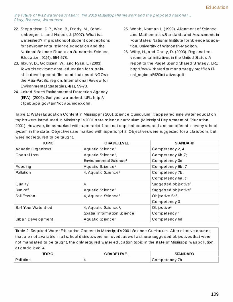
Education

109

Shepardson, D.P., Wee, B., Priddy, M., Schel-22. lenberger, L., and Harbor, J. (2007). What is a watershed? Implications of student conceptions for environmental science education and the National Science Education Standards. Science Education, 91(4), 554-578.Tilbury, D., Goldstein, W., and Ryan, L. (2003). 23. Towards environmental education for sustain-able development: The contributions of NGOs in the Asia-Pacific region. International Review for Environmental Strategies, 4(1), 59-73.United States Environmental Protection Agency 24. (EPA). (2009). Surf your watershed. URL: http://cfpub.epa.gov/surf/locate/index.cfm.

Webb, Norman L. (1999). Alignment of Science 25. and Mathematics Standards and Assessments in Four States. National Institute for Science Educa-tion, University of Wisconsin-Madison. Wiley, H., and Canty, D. (2003). Regional en-26. vironmental initiatives in the United States: A report to the Puget Sound Shared Strategy. URL: http://www.sharedsalmonstrategy.org/files/Fi-nal_regional%20initiatives.pdf


Table 1: Water Education Content in Mississippi’s 2001 Science Curriculum. It appeared nine water education topics were introduced in Mississippi’s 2001 state science curriculum (Mississippi Department of Education, 2001). However, items marked with superscript 1 are not required courses, and are not offered in every school system in the state. Objectives are marked with superscript 2. Objectives were suggested for a classroom, but were not required to be taught.

TOPIC GRADE LEVEL STANDARDAquatic Organisms Aquatic Science1 Competency 2, 4Coastal Loss Aquatic Science1,

Environmental Science1

Competency 6b,7; Competency 3e

Flooding Aquatic Science1 Competency 6b, 7Pollution 4, Aquatic Science1 Competency 7b,

Competency 6a, cQuality 4 Suggested objective2

Run-off Aquatic Science1 Suggested objective2

Soil Erosion 4, Aquatic Science1 Objective 5a2, Competency 3

Surf Your Watershed 4, Aquatic Science1, Spatial Information Science1

Objective2

Competency 2

Urban Development Aquatic Science1 Competency 6d

Table 2: Required Water Education Content in Mississippi’s 2001 Science Curriculum. After elective courses that are not available in all school districts were removed, as well as those suggested objectives that were not mandated to be taught, the only required water education topic in the state of Mississippi was pollution, at grade level 4.

TOPIC GRADE LEVEL STANDARDPollution 4 Competency 7b


110


Table 3: Water Education Content in Mississippi’s 2010 Science Framework. The 2010 Science Framework offered greater potential for water education in Mississippi’s public schools. Ten water education concepts can be introduced via the 2010 Mississippi Science Framework, and all ten concepts can be offered through K-8 portals within the state. The new 2010 Mississippi Science Framework exhibits greater vertical alignment of the curriculum for the potential of reinforced water education concepts across various grade levels. Items marked with superscript 1 are not required courses, and are not offered in every school system in the state. Parentheses indicate that only one of the investigators identified the grade or course portal as having poten-tial for inclusion of the water education concept.

TOPIC GRADE LEVEL FRAMEWORKAquatic Organisms 7

Aquatic Science1

4d3a-f, 4a-c

Coastal Loss 3, 5Aquatic Science1

Earth and Space1

4b2e4d, 5a

Conservation K, 578 Environmental Science1

4d4g4d3a

Flooding 3, 4, 5 3c Groundwater 5

67

4a, 4g4g4a

Pollution 1, 2, 3, 4, 6 Aquatic Science1

4d4a

Quality (5), 6, Environmental Science1

4g3a

Run-off (5), 6 4gSoil Erosion 3, 5,

Aquatic Science1

Earth and Space1

4b2e4d,e

Urban Development 4, 5 (7) Aquatic Science1

4d4g4a

Education

111


Table 4: Comparison of 2001 and 2010 Mississippi Science Frameworks for Water Education Content. Although a direct comparison between the 2010 Mississippi Science Framework and the 2001 Mississippi state science curriculum is not possible, the potential for water education according to topic and grade level are listed for each of the frameworks. Items marked with superscript 1 are not required courses, and are not offered in every school system in the state. We interpret the 2010 Mississippi Science Framework as having more poten-tial for water education, and an improvement from the 2001 science curriculum. Blue cells are those con-cepts that have improved potential in the K-8 classroom under the 2010 Mississippi Science Framework.

TOPIC 2001 MS State Science Curricu-lum—Grade Level and/or Elective

2010 MS Science Framework—Grade Level and/or Elective

Aquatic Organisms Aquatic Science1 7, Aquatic Science1

Coastal Loss Aquatic Science1, Environmental Science1

3, 5,Aquatic Science1, Earth and Space1

Conservation K, 5, 7, 8, Environmental Science1

Flooding Aquatic Science1 3, 4, 5Groundwater 5, 6, 7Pollution 4, Aquatic Science1 1, 2, 3, 4, 6, Aquatic Science1

Quality 4 (5), 6, Environmental Science1

Run-off Aquatic Science1 (5), 6Soil Erosion 4, Aquatic Science1 3, 5, Aquatic Science1,

Earth and Space1

Surf Your Watershed 4, Aquatic Science1, Spatial Information Science1

Urban Development Aquatic Science1 4, 5, (7), Aquatic Science1


112

The Chickasawhay River: A small Mississippi stream vs the U.S. Army Corps of Engineers

Joy Buck, University of Southern MississippiThomas H. Orsi, University of Southern Mississippi

Michael Rasmussen, University of Southern MississippiAndrew Newcomb, University of Southern Mississippi

Garrett Carter, University of Southern Mississippi

There has been recent interest in improving the recreational value of the Chickasawhay River in Clarke County, MS, by removing large wood obstructions from the stream channel. The Pat Harrison Waterways District conducted an initial survey in 2002 and commissioned a follow-up in 2004, determining in both instances, that such a project would be extremely costly and ill-advised. None-the-less, the project proceeded from 2006-2008. Our purpose is not to speculate on whether the project was environmentally or financially appropriate, nor is it an attempted indictment of the agencies involved, past or present. Instead, we look to the historical record, seeking any information that might provide insight into the potential long-term success of a project like that conducted recently on the Chickasawhay.

Interestingly, “improvements” to the Chickasawhay River began over 100 years ago. Initial examination from Subuta to its confluence with the Leaf River began in 1878-1879 by the U.S. Army Corps of Engineers (USACE). This was followed a decade later (1888-1889) with an examination of the reach from Enterprise to Bucatunna. Both surveys concluded that the Chickasawhay was “badly obstructed by logs, snags, overhanging trees, shoals, etc”. Regardless, the stream was considered “worthy of improvement by the United States” and a project began in 1890 to provide for high-stage navigation from Shubuta to the Leaf-Chickasawhay confluence.

Based on available Annual Reports to the Chief of Engineers, there are three general phases of USACE engagement with the Chickasawhay: (1) Improvement (1890-1900); (2) Maintenance (1900-1910); and (3) Depreciation (1910-1915). The Corps begins ambitiously in the 1890’s, removing or cutting up thousands of obstructions from the river as listed in an 1892 report: Overhanging trees felled and cut up - 4500 Number of cuts - 5000 Overhanging trees trimmed - 1500 Logs on bank cut up - 6000

The Corps then gradually realized the scope of the task and the dynamic realities of the Chickasawhay at the turn of the century and adjectives such as “troublesome” and “dangerous” began to be used. Also at this point, USACE redefined the stream reach to be improved and the new section for improvement coincidentally corresponded with the reach they had already cleaned -- the project was pronounced “complete”. All subsequent activity to ~1910 was related to channel maintenance, and it was acknowledged that if maintenance ceased, the stream would quickly return to its original condition. During the early 1910’s, USACE begins to “retreat” and in 1915, presented two arguments to justify the project’s suspension: (1) “No protest against obstruction of the river has ever been received”; and (2) the stream is “commercially unimportant, useful only for logging and rafting.” The Chickasawhay was then declared “unworthy of improvement by the United States” and all future expenditures ceased. So after 25 years, that was that. And now almost a century later, the Chickasawhay is again under the spotlight. But if history is any guide, she is not likely to surrender without a fight.

Key words: Management and Planning, Geomorphological Processes, Hydrology

Management/Planning

Michael E. StovallIbrium Systems Corporation

Sustaining Alabama fishery resources: A risk-based integrated environmental, economic, and social resource management decision framework

C. Elizabeth Stokes Mississippi State University

Identification of pentachlorophenol tolerant bacterial communities in contaminated groundwater after air-sparging remediation

Jason Barrett Mississippi State University

The influences on the capacity development assessment scores of publicly-owned drinking water systems in Mississippi

Man

agem

ent/

Plan

ning


114

Sustaining Alabama fishery resources: A risk-based integrated environmental,

economic, and social resource management decision frameworkMichael E. Stovall, University of Alabama

The natural systems that make-up Mobile Bay, its watershed, and adjacent marine waters serve as critical natural infrastructure supporting water supply, transportation, power generation, recreation, commercial fishing, agriculture, forestry, and a wide variety of other valued uses for the people in the watershed. Development activities and multiple uses have placed signification stresses on the ecosystem and the sustainable use of its aquatic resources. These stresses have impacted the unique marine and freshwater biodiversity of this aquatic system.

This paper presents results of Phase 1 of a NOAA funded assessment of the freshwater and marine fisheries of the Mobile Bay watershed, the related aquatic system and the stresses placed on this system by both anthropologic and natural conditions The project is a collaborative effort among government, corporate, and private stakeholders to build the resource management decision support tools needed to assure a sustainable fisheries and coastal seafood industry for Mobile Bay and its watershed, while balancing statewide environmental, economic, and social demands.

Existing system conditions were initially characterized through review of available literature and agency documents. Two collaborative multi-stakeholder workshops were held in 2009 in order to gain their perspective on the most immediate threats to a sustainable Mobile Bay system. Challenges associated with multi-stakeholder coordination, resource allocation among potentially competing uses, and public education of how human activities potentially impact system health were ranked as higher threats for sustainable system management than more traditional environmental perturbations such as non-point source pollution or aging infrastructure.

Results from Phase 1 studies have identified tentative indicator species, sources of stresses, model boundary conditions and other major system components for Phase 2 activities to develop a preliminary decision support system, which will link riparian, stream, estuary, and near-shore marine conditions responses to various human use activities via selected indicator species monitoring. The long-term project outcome is to design and develop new tools to model and evaluate social and environmental factors that influence management of a sustainable fishery, support man-made infrastructure investment decisions, and provide a common language for expressing goals, processes, and concerns affecting responsible stewardship of Alabama’s fisheries resources.

Recent developments incorporating decision impacts of near-shore drilling will also be discussed.

Key words: Watershed Management and Planning

Management/Planning

115

Identification of pentachlorophenol (PCP) tolerant bacterial communities in

contaminated groundwater after air-sparging remediation

C. Elizabeth Stokes, Mississippi State UniversityM. Lynn Prewitt, Mississippi State University

Hamid Borazjani, Mississippi State University

Pentachlorophenol (PCP), a highly toxic and recalcitrant wood preservative, contaminates groundwater aquifers in many areas of the United States. Improper handling, storage, and disposal practices in the past have led to the contamination of groundwater at many wood treatment facilities. Air sparging, the injection of clean air under pressure into the groundwater system, has emerged as a viable in-situ treatment option for removal of this type of contamination. Previous studies have relied on morphological studies for identification of the bacterial community that is responsible for PCP degradation. However, molecular identification of DNA extracted from the bacterial community present in the groundwater will provide a more accurate description of the microbial community. Groundwater samples from eight biosparging wells were taken quarterly and analyzed for total PCP concentration, nutrient content, and monthly samples were used for microbial identification. Microbial counts were taken for each well on selective media, and changes over time were compared between wells within the sparging wells’ zone of influence and wells not directly impacted by air sparging. PCP concentration was below 1 ppb and nutrient levels were within the normal range. Well 14 (above air injection) revealed Burkholderia sp., Denitratisoma oestradiolicum, Thauera sp., and Rhodoanobacter thiooxydans, along with >40 other species that were listed as “uncultured” in BLAST. Well 51 (below air injection), presented a greater variety of bacterial species than Well 14, including the known PCP degrader Flavobacterium, in addition to numerous “uncultured” species. DNA extracted from other wells is currently being sequenced and T-RFLP analysis is underway to provide a comparison over time of microbial communities between aerated and non aerated wells.

Key words: toxic substances, treatment, ground water, methods, remediation

IntroductionPentachlorophenol (PCP, Penta) is a widely

used wood treatment chemical that is highly resis-tant to degradation. In the United States, its use was restricted in 1997 when it was classified by the EPA as a probable human carcinogen. PCP is still used in the treatment of utility poles in the United States. Prior to regulation, there were a number of issues with disposal of excess chemical, disposal of wood wastes, leakage of stored chemical, and cleanup of spilled PCP. Because of PCP’s strong resistance to degradation, it becomes a very recalcitrant contaminant when introduced to soil or water systems. The relatively recent introduction of PCP in

1936 means that indigenous microorganisms have likely developed PCP degradation mechanisms only in the last 70 years(Crawford 2007). A variety of remediation techniques have been applied to aid in the removal of PCP, and air sparging is one that has been particularly useful. Air sparging is the ap-plication of air under pressure into saturated zones to volatilize dissolved phase contaminants and increase oxygen levels in groundwater (Bass 2000). Air sparging increases both the physical removal and aerobic biodegradation of contaminants, and is especially successful on volatile organic com-pounds such as chlorinated solvents and petroleum hydrocarbons (Bass 2000). PCP’s heavily chlorinated


116

structure makes this treatment an ideal solution for removal of the contaminant without the need to excavate the contaminated soil and without pumping a large volume of groundwater out for treatment off-site.

It is understood that indigenous microorganisms often have the ability to degrade PCP given ideal conditions such as ample nutrients and oxygen. What is not understood, however, is which members of the microbial community are actively involved in the degradation. The identification of the members of a bacterial community that has been exposed to a PCP contamination, and that has undergone a remediation treatment that is beneficial to the growth of the community, is therefore the primary goal of this study. By identifying specific members of the community that are responsible for PCP degra-dation, it is hoped that bioremediation of contami-nants such as PCP can be enhanced.

Materials and MethodsAir Sparging Treatment

In 2000, a series of air sparging wells were installed at a wood treatment facility in Mississippi where a groundwater contamination of PCP had been identified. The wells were placed down-stream of the contaminant, creating a “curtain” of aeration intended to prevent the spread of the contaminant stream into the neighboring aquifer. Monitoring wells were installed at the same time, and the site has been sampled quarterly since the installation. The air sparging wells were connected to a regenerative blower supplying

105 standard cubic feet of air per minute (scfm) at a pressure of 15 pounds per square inch (psi)(Bo-razjani 2005). Wells are made of 2-inch schedule 40 PVC pipe with a 5-foot slotted screen portion at the bottom of each well. The screened section was situ-ated at installation within the base of the saturated zone. This ensures aeration of the entire depth of the contaminated area, providing a zone of influ-ence with an approximate radius of 30 feet. Well depths range from 23 to 29 feet below the ground surface. Injection of air through sparging wells has been continuous to date. Figure 1 shows an aerial view of the study site.

Biological and Chemical SamplingAs stated, monitoring wells have been sampled

quarterly since installation to test a variety of chemi-cal and biological parameters. Chemical testing has included measurements of PCP levels, total Kjeldahl nitrogen (TKN), total organic carbon (TOC), total organic phosphorus (TOP), ortho-phosphate (Ortho-P), and chlorine ion (Cl). Water samples (1L) have been collected from each well at each sam-pling period. Chemical testing has been conducted according to EPA Standard Methods for the exami-nation of water and wastewater. Each measured parameter is either an indicator of the contaminant or its breakdown, or a contributing factor to the health of the bacterial community. Bacterial popu-lations have been counted monthly, using the same sampling method as with the quarterly samples. Bacteria were enumerated by diluting 1ml of water collected from each well by a factor of 100, and plating this dilution on nonrestrictive nutrient agar and selective nutrient agar containing PCP. Differ-ences in the two plate counts indicate differences in the PCP-tolerant and non-PCP tolerant species of bacteria. Colony forming units (cfu) were counted and the cfu/mL for each well was calculated from these numbers.

Beginning in December 2009, 500ml water sam-ples were taken monthly, before and after addition of liquid nutrients introduced after the first monthly sampling. The nutrient amendment was selected to increase the available nitrogen and phosphorus to active bacteria within the system. These samples were not subjected to chemical testing monthly, but reserved for more thorough microbiologi-cal examination to determine the composition of the community responsible for PCP degradation. Samples for quarterly chemical analysis were con-tinued in addition to the monthly samples. Quarterly water samples were divided for analysis, with 200 ml for PCP concentration determination, 200 ml for direct extraction of DNA, and 100 ml for plating on selective media and growing in liquid culture. PCP concentration was determined by EPA Standard Method 3510C. DNA was extracted from the water samples using a WaterMaster DNA Purification Kit from Epicentre Biotechnologies.

Identification of pentachlorophenol tolerant bacterial communities in contaminated groundwater…Stokes, Prewitt, Borazjani

Management/Planning

117

DNA sequencing for identificationWhen poor quality DNA was produced from

the direct extractions from water samples in De-cember 2009 and January 2010, an alternative culturing step was added to increase concentra-tion of viable bacteria. One milliliter of each water sample was added to sterile nutrient broth contain-ing 1ppb (1 µg/L) PCP From these cultures, DNA was extracted using a NucleoSpin Plant II nucleic acid purification kit from Macherey-Nagel. The 16s region of extracted DNA was amplified using bac-terial specific primers and polymerase chain reac-tion (PCR). Primers used in the amplification were 16SFOR (5’AGATCGATCCTGGCTCAG) and 16SREV (5’-GGTTACCTTGTTACGACTT). Amplified products were then cloned into E.coli cells containing pCR 4-TOPO vector using a TOPO TA Cloning Kit for Se-quencing (Invitrogen). The resulting plasmids were extracted from the cells using a PureLink Plasmid Miniprep kit, also from Invitrogen, and sequenced on a Beckman-Coulter CEQ8000 Genetic Sequenc-er. Sequences obtained from the CEQ8000 were subjected to BLAST database searches, and match-es with a greater than 96% identity match and 3 or fewer sequence gaps were accepted as identified species.

ResultsMicrobial counts

Variations were observed in total bacterial counts (cfu/mL) as well as in the PCP-tolerant bacterial counts (cfu/mL) between wells at each sampling period, and for the same well at different sampling periods. This fluctuation may be attributed to changes in subsurface water and nutrient avail-ability, as weather changes impact the site. Figures 2 and 3 show the variation in the eight monitoring wells over the sampling period. There is a significant difference in the variation between PCP-tolerant and Total bacteria from the pre-amendment samples and the post-amendment samples. Pre-amendment total bacteria range from 0 to 450,000 cfu/mL, while the PCP-tolerant bacteria range from 0 to 220,000 cfu/mL. Post-amendment total bacte-ria range from 0 to 700,000 cfu/mL, while PCP-toler-ant bacteria range from 0 to 620,000 cfu/mL.

All wells except well 44 showed no detectable bacterial colonies for the months of January and February. Well 44 is at the greatest distance above the line of air sparging wells, and is least impacted by the injection of air. Monitoring well 41, located furthest below the air injection wells, showed the least amount of bacterial growth over time. Monitoring wells 14, 51, 52, 42, and 43 are definitely impacted by the air injection, as they are within the 30-foot radius of the air injection wells. Wells 41, 17, and 44 are outside the zone of influence of the air injection wells.

PCP analysisPCP was examined for each well at each

monthly sampling point according to EPA Stan-dard Method 3510C. EPA detectable limits of PCP in groundwater are currently set at 1ppb. (Federal Register 1999) Figure 4 shows the variation of PCP in the eight monitoring wells over a three month period in early 2010.

DNA sequencing and identification of speciesTable 1 shows results from two of the eight

monitoring wells. Wells 14 and 51 were chosen for sequencing first because the DNA produced from these two wells was of the highest quality and purity. Only sequences with a greater than 96% identity match and less than 3 sequence gaps were considered positive matches. There were a large number of “uncultured” strains that fit the criteria for positive matches, but were not included in the table because they could not be assigned to a particular genus.

DiscussionThe quantity changes within the bacterial com-

munity may be influenced by natural fluctuations related to weather patterns, or water or nutrient availability within the soil system. Bacterial popu-lations in a particular well varied in number from month to month, and between wells. The differ-ences between bacterial populations for different wells are likely a result of the presence of increased oxygen from the air injection wells, the availability of the contaminant to be used as a carbon source



118

for bacterial growth, and the improved C:N ratio provided by the nutrient amendment. The last point is verified by the doubling of both the total bacteria and PCP-tolerant bacterial counts from pre-amend-ment samples to post-amendment samples. Wells that are further above the air injection site, closer to the original source of contamination, seem to have a more stable population of bacteria than wells that are far below the sparging line, further from the original contaminant source. Therefore, it seems that improving the C:N ratio, in conjunction with the air sparging remediation, is beneficial to bacterial community growth.

PCP concentration analysis shows that the levels of contaminant are relatively stable throughout the remediation area, varying from 0.1 to 1.4 ppb. Using the EPA recommendation of 1ppb as a guideline, and knowing that PCP levels as high as 3.60ppm were measured early in the remediation, we can reasonably conclude that the air sparging reme-diation has been beneficial to this area. Whether the remaining PCP in the system is available to the indigenous bacteria as a food source cannot be determined at this point.

As yet, only two known PCP degraders have been positively identified from sequence analysis. Flavobacterium and Burkholderia have the ability to degrade the chlorinated phenol (Saber 1985; Xun 1996). It is possible that Flavobacterium and Burk-holderia are the dominant PCP-degrading species within the entire system. This may be determined as more samples are sequenced and analyzed for known bacterial species.

To further examine changes in bacterial com-munities by well location, the bacterial DNA col-lected from each well is being used in a terminal restriction fragment length polymorphism (T-RFLP) analysis. Terminal restriction fragments (T-RFs) from fluorescently-labeled, digested 16s PCR products are separated by capillary electrophoresis and visu-alized using the Fragment Analysis program of the Beckman-Coulter CEQ 8000 used in bacterial iden-tification. After performing a peak ratio analysis, this data will show the relative distribution of frag-ment sizes throughout each sample. This analysis will show changes in the bacterial community at each

sampling point, giving a picture of how the spe-cies distribution changes throughout the study site over time. Additionally, gene expression of enzymes specific to PCP degradation will be examined using real time PCR (RT-PCR). This will determine the com-munity members capable of performing each step of PCP degradation, and provide a more thorough understanding of the mechanism of PCP break-down. Research is continuing in this study.

AcknowledgementsThe authors would like to express their thanks

to Mr. Min Lee, Ms. Katie Jenkins, and Dr. Young Min Kang for invaluable assistance in this study. This research was supported by the Mississippi Water Resources Institute, the Forest and Wildlife Research Center at Mississippi State University, and the Missis-sippi State University College of Forest Resources.

References CitedBass D.H.; Hastings N.A.; Brown R.A. 2000. Perfor-1. mance of air sparging systems: a review of case studies. Journal of Hazardous Materials. 72:101-119.Borazjani H.; Diehl S.V.; Britto R.; Lybrand M. 2. 2005. In-Situ biosparging of pentachlorophenol (PCP) contaminated groundwater. Pages 179-182 in W.G. Lyon, J.J. Hong, R.K. Reddy, editors; Proceedings of Environmental Science and Technology 2005(1).Crawford R.L.; Jung C.M.; Strap J.L. 2007. The 3. Recent Evolution of Pentachlorophenol (PCP)-4-monooxygenase (PcpB) and Associated Path-ways for Bacterial Degradation of PCP. Biodeg-radation 18: 525-539.Federal Register, National primary and second-4. ary drinking water regulations. Fed. Reg 54, 1999.Saber D.; Crawford R.L. 1985. Isolation and 5. characterizations of Flavobacterium strains that degrade pentachlorophenol. Appl. Env. Micro-biology. 50(6): 1512-1518.Xun L. 1996. Purification and Characterization of 6. Chlorophenol-4-Monooxygenase from Burkhold-eria cepacia AC1100. Journal of Bacteriology 178(9):2645-2649.


Management/Planning

119


Table 1. Identification of bacteria from two monitoring wells. Species marked with an asterisk (*) are known PCP degrading bacteria.

Well 14 – February 2010 Well 51 – February 2010 Burkholderia cepacia * Burkholderia sp. * Herbaspirillum sp Rhodoanobacter thiooxydans Janthinobacterium lividum Azospirillum irakense Thauera sp. Duganella sp. Collimonas sp. Denitratisoma oestradiolicum Pedobacter insulae Janthinobacterium agaricidamno-

sum Pedobacter duraquae Massilia dura Flavobacterium sp. * Aquaspirillum arcticum Oxalicibacterium faecigallinarum

Figure 1. Aerial view of study site, indicating monitoring wells (MW- #), air sparging wells (unlabeled), and groundwater flow direction (arrows).

Mississippi W

ater Resources Conference

2010120

Identification of pentachlorophenol tolerant bacterial com

munities in contam

inated ground

water…

Stokes, Prewitt, Borazjani

Figure 2. Bacterial enumeration from

pre-amend

ment sam

ples. PCP tolerant bacteria are show

n on the left; Total bacteria on the right.

Figure 3. Bacterial enumeration from

post-amend

ment sam

ples. PCP-tolerant bacteria are show

n on the left; Total bacteria on the right.

t f ~~ .,. .... w .,.

++ ~~ f:~

t f ~~ V, .,. ........

I t :E: :E: ~ ~ V, .,. N N

Colony Forming Units (cfu) / ml

December

January

February

March

April

May

June

July

August

September

December

January

February

March

April

May

June

July

August

September

I-' N W -I'> U, Cl'\ -..J 00 00000000 00000000 00000000 00000000

000000000 .,, 0 ~ ' )>

3 II) ::I c.. 3 II) ::I r+ c:, DJ ~ II) ... iii' n 0 0 ::I iii' "' -a 3 s: 0 ::I ;:;: 0 ::::!. ::I

(IQ

~ "'

t f ~ ~ .,. .... w .,.

+ + ~ ~ .i:,. .... .i:,. -..J

t f ~ ~ V, ,I>........

I t ~ ~ V, .i:,. N N

Colony Forming Units (cfu) / ml

September

December

January

February

March

April

May

June July

August

September

September

December

January

February

March

April

May

June

July

August

September

I-' N W -I'> 0 0 0 0 0 0 0 0 0 0 0 0 0 0 0 0

0 0 0 0 0

u, 0 0 0 0 0

.,, ~ ' )>

3 II) ::I c.. 3 II) ::I r+ c:, DJ n ; ... iii' n 2. 0 ::I II)

"' -a 3 s: 0 ::I ;:;: 0 ::::!. ::I

(IQ

~ iii

Management/Planning

121


Figure 4. PCP variation over nine months. 1ppb is the maximum contaminant load (MCL) set by EPA for PCP in groundwater. Upstream wells – 14 and 44; Intermediate wells – 51 and 52; Downstream wells – 17, 41, 42, and 43.

C 0

,;::

"'

60

so

z 30 C ., V C 0

~ 20 u Q.

10

0

Jan Jan 22 29 1>re posl

PCP Variation in Monitoring Wells

Feb Feb Mar Mar A1>r Apr May May June June July July Aug Aug Se1>1 Oct 6 19 26 17 24 16 23 14 21 11 16 16 23 12 19 29 1>ost pre post p1·e post 1>re l>OSI pre post pre post pre post pre ilOSI pre

- MW14 --MW17 --MW41 - MW42

_.MW43 --MW44 --MWSl - MWS2


122

The influences on the capacity development assessment scores of publicly-owned drinking

water systems in Mississippi Jason Barrett, Mississippi State UniversityAlan Barefield, Mississippi State University

The Capacity Development Assessment (CDA) is a focused survey instrument used to quantify the financial, managerial and technical factors of a water system in Mississippi. The survey’s primary focus is identifying the extent to which water systems are complying with Mississippi State Department of Health-Bureau of Public Water Supply regulations and standards. Since the majority of the factors for publicly owned water systems (municipal systems and water associations and districts) measured in the CDA are either directly or indirectly influenced by board management decisions as well as other, more macro/regional external influences such as per capita income, water system population, county population, operator experience, etc., we propose to examine causal influences on the CDA score. Identification of these influences could lead to future local and state policy implementation and educational efforts to strengthen public water systems.

Key words: Economics, Water Supply, Management and Planning

Delta Groundwater

Charles L. Wax Mississippi State University

Refining effective precipitation estimates for a model simulating conservation of groundwater in the Mississippi Delta Shallow Alluvial Aquifer

Jeannie R.B. Barlow U.S. Geological Survey

Water use conservation scenarios for the Mississippi Delta using an existing regional groundwater flow model

Joseph H. Massey Mississippi State University

Water-conserving irrigation systems for furrow and flood irrigated crops in the Mississippi Delta

Heather L. WelchU.S. Geological Survey

Occurrence of phosphorus in groundwater and surface water of northwestern Mississippi

Del

ta G

roun

dw

ater


124

Refining effective precipitation estimates for a model simulating conservation of

groundwater in the Mississippi Delta Shallow Alluvial Aquifer

Charles L. Wax, Mississippi State UniversityJonathan W. Pote, Mississippi State UniversityRobert F. Thornton, Mississippi State University

The shallow alluvial aquifer in the Mississippi Delta region is heavily used for irrigation of corn, soybeans, and cotton, as well as for rice flooding and filling aquaculture ponds in the prominent catfish industry. Water volume in the aquifer is subject to seasonal declines and annual fluctuations caused by both climatological and crop water use variations from year-to-year.

Available climate, crop acreage, irrigation water use, and groundwater decline data from the 19 counties in the Delta were used to construct a model that simulates the effects of climatic variability, crop acreage changes, and specific irrigation methods on consequent variations in the water volume in the aquifer. Climatic variability was accounted for by predictive equations that related annual measured plant water use (irrigation) to total growing season precipitation amounts. This derived relationship allowed the application of a long-term climatological record (50 years) to simulate the cumulative impact of climate on groundwater use for irrigation.

The relationship between rainfall and anticipated crop water use was initially estimated by a simple regression between total growing season rainfall and measured irrigation water use for the period 2002-2007, with a resulting R2 value of 0.93. Adding data from 2008 caused R2 to drop to 0.63. It was recognized that total growing season rainfall was not representative of the timing, or episodic nature, of rainfall compared to plant water demand day-by-day through the growing season. To account for this timing issue, weekly rainfall amounts were compared to weekly expected crop water demand to produce an effective rainfall estimate. The resulting improvements are shown. This effective rainfall compared to irrigation use is expected to provide a much-improved rainfall-irrigation coefficient for use in the model.

Key words: Climatological processes, Groundwater, Irrigation, Management and Planning, Water Use

Introduction Agricultural producers in Mississippi are increas-

ingly relying on irrigation to insure that crops receive the right amount of water at the right time to en-hance yields. The shallow alluvial aquifer is the most heavily developed source of groundwater in the Mississippi Delta region and the entire state (Figure 1). The aquifer is heavily used for irrigation of corn, soybeans, and cotton, as well as for rice flooding and filling aquaculture ponds in the prominent cat-fish industry. Demand for the groundwater resource continues to grow at a rapid rate (Figure 2).

Water volume in the aquifer is subject to sea-sonal declines and annual fluctuations caused by both climatological and crop water use variations from year-to-year. These declines can be dramatic and are most notable during the period April-October of each year, particularly in years when normal crop water demands are accentuated by concurrent abnormally dry climatic conditions. Recharge during the remainder of the year has recently been insufficient to restore water volume, and the aquifer is now being mined at the approxi-mate rate of 300,000 acre-feet per year (Figure

Delta Groundwater

125

3). To underscore the critical nature of this water problem, the most recently documented water vol-ume decline in the aquifer (October 2005-October 2006) is estimated at 500,000 acre-feet (Pennington, 2006). This may represent a worst-case situation in which severe drought combined with consequent increased demand for irrigation. It is estimated that water use for row crops doubled during this period (Pennington, 2006).

It is of critical importance to understand how climatological variability and cultural uses of the water cause the groundwater volume in the aqui-fer to vary. It is also critical to discover and imple-ment management strategies to change irrigation methods and to use precipitation and other surface water sources as substitutes for aquifer withdraw-als and thereby reduce the use of groundwater in the region. Stopping the consistent drop in water volume in the aquifer will require a curtailment averaging about 300,000 acre-feet of groundwa-ter use each year, and the highest priority of this research project is to find and recommend solu-tions to this problem. This information is essential to agricultural producers in the region and to planners in the Yazoo Mississippi Delta Joint Water Manage-ment District who must design sustainable water use scenarios which will allow continuation of the productivity of the region.

The objective of this research is to develop a model that can be used as a management tool to find ways to meet the needs for water use while conserving groundwater. This is the third phase of the project to meet these objectives. In phase one of the project, the growing season precipitation was used to develop a relationship that estimated irrigation use, and this was the driving mecha-nism of the model that simulated water use to the year 2056. Phase two added the use of surface water when growing season precipitation was 30% or more above normal. In this third phase, a new climatological input was introduced into the model—irrigation demand. Irrigation demand was calculated using daily precipitation, evaporation, and a crop coefficient to estimate daily water needs by crop type. Daily values were summed to one week segments which were added to derive

the total growing season irrigation demand. Weekly summations increased temporal resolution, improv-ing model efficiency in accounting for excess daily rainfall, allowing the model to apply excess rainfall in subsequent days.

Background InformationAgriculture is the major water consumer in the

southeast region, and aquaculture specifically has the potential to become disproportionately consumptive. For example, most row crops in the region require 30-40 cm/yr, whereas catfish farming requires up to 100 cm/yr under current practices. In the Delta region of Mississippi where nearly 60% of U.S. farm raised catfish are produced, catfish pro-duction accounts for about 28% of all water used (Pennington, 2005).

Research to reduce reliance on groundwater in aquaculture has shown remarkable potential reductions in groundwater through use of manage-ment strategies to create storage capacity which can capture rainfall to keep ponds filled. For ex-ample, studies show the potential to reduce con-sumption of groundwater in delta catfish ponds by nearly 70% annually through precipitation capture (Pote and Wax, 1993; Pote, et al, 1988; Cathcart et al., 2006). Extension Services in Alabama and Louisiana include variations of those strategies as industry best management practices for reducing groundwater use in those states (Auburn University, 2002; LCES, 2003). In rice production, straight levee systems and use of multiple inlets have been shown to be specific irrigation methods that significantly reduce water use (Smith et al., 2006). Intermittent (wet-dry) irrigation has been shown to reduce water use and non-point source runoff by up to 50% with no yield losses in Mississippi field trials (Massey et al., 2006). Massey (Personal Communication, 2010) states that conserving one inch of pumped ground-water saves producers 0.7 gallons of diesel per acre or 34 kilowatt hours of electricity per acre.

MethodsIn order to assess the change in volume of

water in the aquifer, it was necessary to collect climatological data, crop coefficient formulas, crop

Refining effective precipitation estimates for a model simulating conservation of groundwater… Wax, Pote, Thornton


126

data, and water use data for the growing sea-son. Growing season was defined as May through August. In this study, all but the evaporation data were collected and analyzed for Sunflower County only. It was assumed that climate and cultural land uses (crops, acreages, irrigation methods) in Sunflower County were representative of the entire Delta region. These data were used in a model that was developed to identify and account for relationships between climatological variability and cultural water use. The model is interactive, allow-ing the user to change input values and alter the final output, thus allowing for specific scenarios to be simulated. Successive alternative combina-tions of variables were simulated with the model to determine possible methods and strategies to aid in groundwater conservation and management.

Climatological DataThe precipitation record from Moorhead, MS

(located centrally in Sunflower County) and the evaporation record from Stoneville, MS were used in the analysis. The data were arrayed in an Excel spreadsheet, and missing data were identified. Gaps in the data were filled with data from the next-nearest climate station location. The result was a serially complete and homogeneous daily record of precipitation and evaporation from 1961-2009. The evaporation data were used to represent potential evaporation (PE), or the demand of the atmosphere for water. To include consideration for the physiological demand of different crops at dif-ferent phenological stages, the PE was modified by crop coefficients.

Crop coefficient formulas

The SCS (1970) established consumptive crop use coefficient curves for a variety of crops. Ranjha and Ferguson (1982) matched these values with curves of best fit and derived the following equa-tions to calculate a crop coefficient for three crops, using crop age in days from emergence as input:

CC (Soybeans) = 0.21-(2.97)(DAY)10-3+(4.74)(DAY)210-4-(4.03)(DAY)310-6

CC (Corn) = 0.12+(0.01)(DAY)+(0.18)(DAY)210-3-(2.05)(DAY)310-6

CC (Cotton)= 0.11-(0.011)(DAY)+(0.55)(DAY)210-3

-(3.49)(DAY)310-6

Crop Data

Crop data for cotton, rice, soybeans, corn, and catfish were collected from the U.S. Department of Agriculture’s National Agricultural Statistics Service (NASS). For the five crops, total acres and total ir-rigated acres were retrieved for the years 2002-2009 (the only years for which water use data were avail-able). The percentages of each type of irrigation or management method used for each of the five crop types in 2006 are shown in Table 1.

Water Use DataWater use data were supplied by Yazoo-Missis-

sippi Delta Joint Water Management District (YMD) in acre-feet/acre (A-F/A). For 2005 through 2009, these data were divided into the amount of water used by each specific irrigation method for cot-ton, corn, soybeans, and rice (as determined by a survey of about 140 sites monitored by YMD shown in Figure 4), as well as the total average water use for each of the crops. For 2002-2004, only the total average water use amount for each of the four crops was provided. Therefore, a ratio based on the 2005-2008 specific irrigation methods-to-total average water use from 2002-2004 was formulated to identify relationships between the given aver-age water use and constituent water use amounts associated with each specific irrigation method for each crop for the years 2002-2004 (Merrell, 2008). As an example, Table 2 shows that furrow irrigation water use for cotton in 2007 was 0.53 A-F/A. The to-tal average water use for irrigation in 2007 was 0.50 A-F/A. Furrow water use was then divided by the total average water use (0.53 A-F/A / 0.50 A-F/A) to get the furrow-to-average water use coefficient of 1.06. The same procedure was used for the pivot irrigation method. The ratio was calculated for the years 2005—2008, and the average of those four years is used as the specific irrigation coefficient for cotton in the model.

Catfish water use is dependent upon whether the producer uses the maintain-full (MF) or the drop-add (6/3) management scheme. Only total


Delta Groundwater

127

average water use by catfish ponds was provided by YMD, also in A-F/A, and only for 2004 and 2006. So, the catfish water use model developed by Pote and Wax (1993) was used with the Moorhead cli-mate data to estimate the amounts of water used by each of the management schemes in Sunflower County for the period 1961-2009. A ratio between the total average water use and the water use associated with the two possible management schemes in catfish ponds was developed, similar to the water use amounts determined for the specific irrigation methods of the row crops and rice. As shown in Table 3, an average of the four years for which measurements were available was calculat-ed to obtain the percentage of water use by each of the management schemes.

These water use data for row crops, rice, and aquaculture were combined with acreage data to calculate the total amount of water used for irriga-tion for each crop in the county in 2006. This analysis provided an evaluation of water use by crop type which was the basis for developing a static model. The static model was used as a standard against which all other scenarios of climatic variability, land use and management changes were compared.

Irrigation demand-water use relationshipRecognizing that the amount of rainfall during a

growing season significantly influences the amount of irrigation needed, a method was developed to account for this climatological variability. Total growing season precipitation was initially used, but problems with timing and distribution of rainfall through the growing season led to a weak relation-ship in some years. It was therefore decided to increase the resolution of the model and therefore refine effective precipitation estimates by examin-ing moisture deficits and surpluses on a daily basis.

In addition to atmospheric demand (evapora-tion), crop water demand was introduced into the model by use of a crop coefficient relating crop water use to phenological stage. Evaporation data and the crop coefficient combine the climatic de-mand and crop demand to estimate the total daily demand for water. Irrigation demand is derived for each day by subtracting the calculated daily total

demand for water from daily precipitation. Daily accounting of water demand resulted in

the use of only rainfall needed to satisfy each day’s specific irrigation demand, discarding the excess rainfall for that day. In reality, the environment does not “restart” each day; that extra moisture would be saved in the soil and applied to the next few days’ water need, reducing the irrigation de-mand over those few days. In order to more accu-rately model actual field practices, daily irrigation demand values were summed by weeks through the growing season, capturing the “excess” rain-fall on any day and thereby reducing the weekly demand for irrigation. The weekly values were then summed to get a total seasonal irrigation demand. This more realistically calculated irrigation demand was regressed against actual seasonal water use, as measured by YMD, to find the relationship to predict actual water that will be used in any year. Calculated seasonal irrigation demand is now used as the climatological variability input to drive the model.

Table 4 shows how growing season calculated irrigation demand was regressed against measured total average water use for cotton, corn, soybeans, and rice for 2002-2009 to develop the function for estimating the amount of water use by crops based on the amount of irrigation demand. Figure 5 shows a comparison of measured water compared to the water use calculated by this method for the row crops and rice for the period 2002-2009. Figure 6 shows an example of calculated irrigation de-mand for Corn from1961-2009, and compares the calculated demand against the measured irrigation from 2002-2009. Catfish water use was obtained from model-estimates based on daily rainfall rather than total growing season rainfall. In this manner, water use by all five crops was linked to climatic variability each year.

Model developmentThe purpose of this research is to determine

causes of short-term aquifer declines resulting pri-marily from cultural water uses and climatological processes. The climate data, crop data, water use data, and irrigation demand - water use relation-



128

ships were used to develop a model that could assess water volume declines in the aquifer over a growing season. Based on crop average water use relationships in effect in Sunflower County in 2006, the model calculated amounts of water taken from the aquifer by each specific irrigation method and management method for each of the five crops. The model then summed the specific water uses for each year, resulting in a total annual reduction in the volume of water in the aquifer.

Using the 2006 Sunflower County land use and crop water use relationships with irrigation demand-water use relationships developed for each crop, calculated irrigation demand from the past 49 years (1961-2009) was used as a variable in the model to estimate the total water use for each year 49 years into the future (2008-2056). The aver-age of the annual recharge volumes measured in the aquifer between 1989-2009 was then used with the modeled water volume declines each year to characterize the cumulative water volume changes over the 49-year period. The model was subsequently used to simulate different scenarios of water use by changing crop acreages or irriga-tion methods from the static 2006 data, permitting assessment of changes in water volumes over time under different land use and management condi-tions. Consequently, the model was used to formu-late recommendations for monitoring and manag-ing water volume changes in the aquifer.

ResultsThe model is an interactive Excel spreadsheet

consisting of 49 blocks with each block represent-ing one year (Figure 7). Each block is comprised of 13 rows and 15 columns. It is interactive through column ‘G’ with columns ‘H’ through ‘O’ contain-ing formulas based on the information entered in columns ‘A’ through ‘G.’ Single or multiple variables can be changed to alter the overall water use amount given in cell ‘O13.’

Results of the first 48-year model simulation (2008-2055) using Sunflower County 2006 static cul-tural water uses for each year (Table 1) with rainfall recorded from 1961-2008 are shown in Figure 8. In this scenario, it can be seen that water volume in

the aquifer begins at a little more than negative 200,000 A-F and consistently drops to about nega-tive 600,000 A-F in the first eight years. The draw-down stabilizes and water volume even rises be-tween about 2015-2040, then water volume again drops consistently to about negative 1,600,000 A-F during the period 2041-2055. Subsequent simula-tions were conducted with alternative scenarios of land uses, irrigation methods, and management strategies employed.

Figure 9 shows the results for that 48-year period when water use practices were changed to reflect the most conservative water use method for each crop: 100% pivot irrigation for cotton; 100% zero grade for rice; 100% pivot for corn; 100% zero grade for soybeans; and 100% 6/3 management strat-egy for catfish. It can be seen that these changes resulted in consistent recovery of water volume beginning after the first year of these practices, ending in 2055 with a positive volume of around 2,900,000 A-F.

Figure 10 shows the results for that 48-year period when water use practices were changed to reflect the most consumptive water use methods for each crop: for cotton,100% furrow irrigation; corn 100% straight levee; rice 100% contour levee; soybeans 100% pivot; and catfish 100% maintain full. These changes resulted in consistent water volume declines from the beginning of the 48-year period, ending at about negative 4,200,000 A-F in 2055.

Figure 11 shows results of using surface water in lieu of groundwater in combination with the use of the new irrigation demand as the climatological driver for the model for the 49-year period 2008-2056 (and incorporating the wet year 2009). Using surface water for 25% of irrigation demand when growing season rainfall was 30% or more above average resulted in consistent declines in water volume from the beginning of the period until about 2017. During this 10-year period there were no years in which growing season precipitation met the 30% above normal threshold. From about 2017 to 2044 water volumes in the aquifer increased or stayed level, well above what the volume would have been each year if no surface water had been used. Beginning in 2044 another group of years oc-


Delta Groundwater

129

curred when the precipitation did not meet the 30% threshold and water volumes declined accordingly until the end of the period, but still ended about positive 1,000,000 A-F above the static scenario.

ConclusionsThe model is a sensitive tool that is useful for

various forms of analysis. Growing season irriga-tion demand, in place of total growing season rainfall, can be used to more effectively simulate inter-annual climatological variability through time. Crop acreages and irrigation methods, including use of surface water when available, can be used to account for cultural influences on water use through time. This combination of climatological and cultural drivers of groundwater demand can be used in the model to determine best and worst case scenarios in overall groundwater use in the aquifer. Results indicate that the aquifer responds to small changes in water use associated with crop type, irrigation methods, and use of surface water when available. Results also show that the aquifer water volume is apparently very strongly related to changes in water use methods associated with climatological variability.

Figure 12 shows how often precipitation could supply crop water needs for each of the row crops and rice through the 49-year period by comparing calculated irrigation demand and total growing season precipitation. The bars above the mid-line represent years when the climate delivers “extra” water, more than the crops can use. These are years when the extra, or surplus, water could be stored. The bars below the mid-line represent years when rainfall is not sufficient to meet the needs of the crops. In these years, 100% of the water de-livered by the climate is used and the crop needs must be supplemented with groundwater irrigation.

The analysis concludes that climate could provide the entire water need of the plants in 70% of the years for corn, 65% of the years for soybeans and cotton, and even 5% of the years for rice. Even though the distribution of the extra water through the growing season may rule out total dependence of producers on this source of water, this analysis does demonstrate that extra water delivered by

the climate could be a source of water that could be used often in place of pumped groundwater. Instituting this practice could save energy, save producers money, and enhance the sustainability of the aquifer.

References CitedAuburn University, 2002. Auburn University and 1. USDA/Natural Resources Conservation Service, Managing Ponds to reduce Effluent Volume, BMP No. 21. (http://efotg.nrcs.usda.gov.refer-ences/public/AL/G02ReduceEffluent.pdf)Cathcart, T.P., C.L. Wax, J.W. Pote and Sugeng 2. Triyono, 2007. “A Climatological Basis for Con-serving Groundwater and Reducing Overflow in Aquaculture Ponds in the Southeast United States.” Aquacultural Engineering, 36(2007)225-232.LCES, 2003. “Aquacultural Production Best 3. Management Practices (BMPs)”, Pub. 2894 4/03 (Online only). Louisiana Cooperative Extension Service, Baton Rouge, LA.(http://www.agctr.lsu.edu/NR/rdonlyres/4005CC33-BF01-4FAB-8EA3-E2D9ABCE038C/2616/pub2894aquaBMP6.pdf).Massey, Joseph H., 2010. Associate Professor, 4. Plant and Soil Sciences, Mississippi State Univer-sity. Personal communication, November, 2010.Massey, J.H., M.C. Smith, A. Johnson, 5. J.Thomas, P.L.Tacker, E.D.Vories, S. Lancaster, A.A.Andrews, and P.Ampim, 2006. Multiple-Inlet plus Intermittent Rice Irrigation Increases Rainfall Capture and Reduces Non-Point Source Runoff. Proceedings, 31st Rice Technical Working Group Meeting. The Woodlands, TX. Merrell, Tia L., 2008. “Development of an Inter-6. active Model Predicting Climatological and Cultural Influences on Annual Groundwater Volume in the Mississippi Delta Shallow Alluvial Aquifer.” MS Thesis, Mississippi State University.Pennington, Dean, 2005. 2005 Annual Report, 7. Yazoo Mississippi Delta Joint Water Manage-ment District, Stoneville, MS 38766.Pennington, Dean, 2006. Executive Director, Ya-8. zoo Mississippi Delta Joint Water Management District. Personal communication, October 31, 2006.



130

Pote, J.W., C.L. Wax and C.S. Tucker, 1988. 9. Water in Catfish Production: Sources, Uses, and Conservations. Special Bulletin 88-3, November 1988, Mississippi Agricultural and Forestry Experi-ment Station, Mississippi State, MS.Pote, J.W. and C.L. Wax, 1993. “Modeling the 10. Climatological Potential for Water Conservation in Aquaculture.” Transactions of the American Society of Agricultural Engineers, Volume 36 (5), 1343-1348. Ramkja, A.V. and K.A. Ferguson. 1982. On-farm 11. irrigation scheduling by computer simulation in Arkansas. Presentation, ASAE Southwest Region Meeting, April, 1982, Shreveport, LA.

Soil Conservation Service, 1970. Irrigation water 12. requirements, Technical Release No. 21, U.S. Department of Agriculture, Washington, DC.Smith, M.C., J. H. Massey, P. Tacker, E. Vories, D. 13. Pennington, J. Epting, and C.Wilson, 2006. Water use estimates for various rice production systems in Mississippi and Arkansas. Irrigation Science (DOI 10.1007/s00271-006-0041-0; pgs. 1-7).


Table 1: Irrigated acres and type of irrigation or management method used for each crop type in Sunflower County, 2006

CropAcres

irrigated% furrow

% straight

% pivot%

contour% zero grade

% multiple

inlet% MF % 6/3

cotton 60,300 81 19rice 27,600 56 20 12 12corn 8,910 100soybeans 86,350 49 50 3 6 2catfish 24,300 34 66

Table 2. Development of specific irrigation coefficients: cotton exampleTotal Avg(A-F/A)

Furrow(A-F/A)

Pivot(A-F/A)

Furrow to Avg

Pivotto Avg

2008 0.60 0.60 1.002007 0.50 0.53 0.40 1.06 0.802006 0.84 0.89 0.62 1.06 0.742005 0.51 0.55 0.42 1.08 0.82

1.05 0.79

Table 3. Explanation of catfish management scheme water useEquation: MFx + 6/3 (1-x) = Total Water Use (A-F/A)

MF 6/3 Total X 1-X2004 3.16 0.53 1.45 0.35 0.652006 3.52 1.56 2.4 0.43 0.572007 3.65 1.03 1.9 0.33 0.672008 3.35 0.79 1.4 0.24 0.76

Average 0.34 0.66

Delta Groundwater

131


Figure 1. Distribution of permitted wells in Mississippi, 2005.

,. . ..... . .. ~ .. . . . .. ..

' . : ,-·. • . • • • . ...... ., . ~

•· .. ..

• • ' • .. •

.,

• 4~ .. •• . • •• i ..

.. :

• • • ~--·

.. ♦ • .I • I • 1'

.••'S. ~~-,:. ..... J:.!'.,:J ., . . -~. . .. t:---':-, ....;.r .• , Y. • • • • • • • -.i- . .... ,~.," ,. .,

•• ....

+ . . ~ .... . • -'\ .

. . . .. . .. ., .. . . .. . . -- •.. i . .. . .,,.

•:

. : ..

• .. ,.. .

•

•. •.:. ,. ... .

.. : .. .;. · .. --., . . . , •

: -.... • .. . •• . . ·. . .

•. . .. • .. :

. .

• : •·.,•·· . • . . : I .. •

• . ': :• . ... ....

. • •• , ,,t_•

• '"R .... .. .

.

• .. . . .. .

• • t : , - \. •·'-· ~ .,_.,, . , .. ,. .

I : •

. -'":• . . • . t · . :

. . • I • •

:; .. I •'

. .

' ·, . ; c \ ,. .. . . ·~ .. .. . ,.

• ..

•

•


132


Figure 2: New Permit Requests, 2006.

,;;;: - I • l • • / ,__.

I • i -~ r--·

'> (

• ••

J T= • ✓ · .. ~ ~\ - ...;· -.,

i-, -,-,• . - .- '·.._,

) . . . ' \ . . ... ~-('\. e- • •• _. •..., . .,.. ,.., .~ • , ~. "

( ,-/ -· -~ ..... ; } • • e I • • ~ r •· fu rf"" • e ._ • • • I r,$ . .. ' ,. •.. .. . ( .I$ \ • · " ~- _.,,,.. •• -

~ J • •• , .... -1 • .... , -. . . . _.,, . ' . • t I • ~ ) • , ,..- \

...... -~· · • • ~ t' \ • • • • • •JI J \ .•--;- .. , . _.-.c~ J , ~ ..... .. • • • • • • • • ~ i• -··· , ~ ·• • • • ' " • r . . . ~•1. . . ~J , . ; • • _,.. --· 'I.: ' ~ )

. . .. ~ . . ( \

# • _ ... . , . . . . . ..... ·-. .::.....• ) ·-· L.) ••• , __. . ... .... .....i: · ~ • .,. ·.• e v. ~. . \ ·~-c;:: ,,_' ••• • •• e > I l

. • - .• ..... • ' • .. -~ ·-- .:: ..... •• ·t c- ~ •e .. '-ll, • • • • • . I '"'-t"". • • • • .,.... ' • ,_ ~ A,._-. I • ' • / . -.. ------- ~~ ' , • • 1,'-'•l • I r::"- • ) .... ~ . ~ .• ;....,;. . / ·-

I • . ·~-· ~.; ·. / ,.,_

) "_-::; • ' •• 7, / . """' . . .. )

/

• -- . , • • •1/ • • at I •~~ • ,.-~ .. . .' . ...,..,, •.. '/' '°' ...... I I~ ~ • / y.,, - • .r. • )'- . /,• • •N ~ (. >~ .i ' -~

J'\'. ., ,.:;f;-·~c...-· •·' •·7/ I '-. f' '- -- i: .........._,, y . .. . /.· ,.-.,.

-'-=----

- -

20 -..__;;;,---0 10

Scale

Delta Groundwater

133


Figure 3: Seasonal Cumulative Aquifer Volume Decline, 1990-2006.

Delta Aquifer Cumulative Seasonal Change 2,000,000 ~----------------------~

1,500,000 -t---/r.-----ir-.--------------------------1

1,000,000 +-~ ~ drf-+--------------------1

500,000 +-------4:,~~~ \-----------------l

~ o -i-,.-rr-,-,---.-rr,-rr-r\1!'~~17:--rxr-r-,-,-,-,-,--,-rr-rr---.-rr-,-,---r-j ,e °' -500,000 t-----------___;;::tt...:l:;::--------------1 .. ~ 1,000,000 +-------------+-,~ ...... a::::!lt"'"---ft----l

-1,500,000 +--------------=---+-A-~r-1-~..!/J--\---A-- -l

-2,000,000 +----------------ll--------~-,,&-+l

-2,500,000 +------------------------¥--! -3,000,000 ...__ ______________________ ____,

Year


134


Figure 4: Locations of Water Use Survey Wells, 2006.

Locations of the 2006 Water Use Survey Wells

Water Use Shea

.Cotton

QCom

eRlce

-• •

Plr!O

Delta Groundwater

135


Figure 5. Comparison of calculated and measured water use.

Figure 6: Calculated (1961-2009) vs. Measured (2002-2009) Corn Irrigation (Y=1.180774(x) + 0.001839; R2=0.77)

<

Cotton

4.00

~ 3.00 LI. 2.00 • < 1.00 • • • a a • ' .. 0.00 '

s9, ,# ,# ~ ~ ~ f:,'lJ ~ '1,c:s ti; ti; '1,<:s '1,c:s ,fl '1,<:s ,fl

1 ~ Cck!Jated lmgalt0n ~ Measued lmga:ion (YMO) I

Corn

4.00 ..--------------, ~ 3.00 ---------------i ":- 2.00 <( 1.00 ■ ■ i t ■ e • ,e

0.00

4

3.5

3

2.5

'6>~ '6><:>":, '6><:1- '1,# '1,~<o '1,<::,'S '1,<::,c'P '1,<::,~

j ~ carua1ed lrnga,on ----Meas1Jed lmga,on (YMO) I

:;: 2 <

1.5

0.5

0

-

I . I

Soybeans

4.00

~ 3.00 LI. 2.00 • < 1.00 • ' I • a • • a 0.00

'1,<::,<1-- '1,<:>,$> '1,<::,<J' '6>,g, '6><:><o '1,<::,~ '1,<:><:>'b '1,<:><::,0)

I --cacu81ed lnigation --Meoswed lrriga<ion(YMD) I

Rice

4.00

1 ~ ~ ~ 3.00 a a • ' • • ~ 2.00 < 1.00

0.00

I ~ C-cUated lmga,on _.,__Measuedlm9al1on(YMO) I

. - . I I . I •


136


Figure 7: Model illustration using 2008 climatological data to estimate water use in the year 2055.

A 8 C D E F 1 2008/2055 2 Total Acres 3 COTTON % furrow % pivot 4 60300 0.81 0.19 5 RICE % contour % straight % Ml % ZG 6 27600 0.2 0.56 0.12 0.12 7 CORN % furrow % pivot % Sir % ZG 8 8910 1 0 0 0 9 SOYBEANS %furrow % straight % pivot % contour % ZG 10 86350 0.49 0.4 0.03 0.06 0.02 11 CATFISH % MF % 6/3 12 24300 0.34 0.66

J K L M

Furrow Use Pivot Use 0.491450139 0.369757724

Con Use St Use Ml Use ZG Use 3.62651423 3.17694635 2.667436086 1.678386751

Furrow Use Pivot Use Sir Use ZG Use 1.24669936 0.582569794 1.38651611 0.827249108

Furrow Use St Use Pivot Use Con Use ZG Use

G H

GS Precip Seasonal ID 18.69 0.46804775

18.69 2.9971192

18.69 1.16513959

18.69 0.92303002

N

Water Used 28240.21337

83514.60657

11108.0913

0

1.043023924 0.803036119 0.904569421 0.83995732 0.526127112 79472.50179 MF Use 6/3 Use

3.3525 0.785833333 40301 .55 242637

Delta Groundwater

137


Figure 8: Model Result when land use and irrigation methods are held constant as observed in 2006 in Sunflow-er County for the 48-year period

Figure 9: Model results when land use and irrigation methods are changed to reflect adoption of the most conservative irrigation method

IL

~ 1i ,! .. ~ u C

IL

~ 1i ., -.. ~

u C

0

-200000

-400000

-600000

-800000

-1000000

-1200000

-1400000

-1600000

-1800000

"' "' C) C) C) ~

"'

Cwnulalh-e Aquifer Cba11&e '.\IodeDed 2008-2055 (2006 Sunflower County I.and t:se Held Constant)

"' "' "' "' C) C) C) C) ~ ..., "' - ..... C) w

,._, ,._, N N ,._, QC)C)QC) ..., ..., (.,,) w (.,) CD <.O N U"I QO

Year

I- STATIC!

..., "' C) C) ,. ,. - ,.

'.\!lost ConservaliYe Irrigation '.\1etbods Implemented (Cotton 100'9 Ph"01,tR.ic.e 100'9 Z.C, Cera 100'9 Pi.t"OC, So)i>eam 11)()% ZC, Cadi&b 10<.M 613)

3500000 ~----------------------~

3000000

2500000

2000000

1500000

1000000

500000

0

-500000

-1000000

-1500000

"' ...,

"' ...,

"' "' "' "' "' "' ...,

"' ...,

"' "' "' C) C) C) C) C) C) C) C) C) C) C) C) C) C) C) C) C) - "' "' "' "' w w w ~

,. - "' u,

"' ,. ..... C) w a, <D "' "' "' ,. ..... C) w

Year

1- CK'.NGE - STAn:: I


138


Figure 10: Model results when the most consumptive irrigation methods and management strategies are used.

Figure 11: Model results 2008-2056 when surface water irrigation is implemented and irrigation demand is used as the climatological driver.

u. ~

i .... ~ <

)lost Consumptive Irrigation )Ietbods Implemented (Coa oo 100'9 F\U"l"Off, Rice lOO¾ Cootou.r1 Corn 100'9 Str»&bt, So,·beaos l OOli Pl\'Ot.

C.tfuh 10014 Mf) 0 .,,..,,.,,...,,....,,..,,.....,.,,.......,....,..,,...,.,.......,.,.,.,,.,...,.,..,.,.,,.,.,.,,.,...,.,,,,.,..,,.,.,.,,.,...,.,,,,..,,..,.,.,.,,.,,...,.,,,..,,..,.......,

-500000

-1 000000 -1---.!.lL~ rr-,------------....!.!t.lL'IAf!-I/J,/l,......i _ -1500000 +---------'..!..!.~ r,r-;--,----------------1 "-~ -2000000 +---------2-l"A,frr-:-------------1 'S .! -2500000 -1-----------------'~¾11.---------l

~ -3000000 +------------------= ¥,,~ -----1 ,c

-3500000 +-------------------'--""'"bt.-:------1 -4000000 +--------------------~AA!

-4 500000 -'-------------------------'

0

-200000

-400000

-600000

-800000

-1000000

-1200000

-1400000

-1600000

-1800000

"' ~

,...,,...,,...,,..., C) C) C) C)

0 -0) ... ....

!:l !:l !:l "' ~ ~ ~ § ~ Js .....

"' "' "' "' "' "' "' "' "' "' "' "' 0 0 0 0 0 0 0 0 0 0 0 0

"' "' "' "' w w w ~ .. .. "' "' 0 w 0, <D "' "' 0) .. .... 0 w Year

I- CHANGE - STATK:I

~ ~ !:l !:l "' ~ !:l !:l "' ~ ll:l I$ 8 ii,. t ~ (,) Ol 0, CD ~ 0

Year

I- STA TIC - SFCWA TER I

~ (,)

Delta Groundwater

139


Figure 12: Effective precipitation—years in which climate delivers a surplus or a deficit of precipitation to meet crop water needs.

25

20

15 ·

10

5 II) G> ,:;; <.> E

-5

-10

-15

-20

-25

lo Corn CJ Soybean □ Cotton ■ Rice I


140

Water use conservation scenarios for the Mississippi Delta using an existing regional

groundwater flow modelJeannie R.B. Barlow, U.S. Geological Survey

Brian R. Clark, U.S. Geological Survey

The alluvial plain in northwestern Mississippi, locally referred to as the Delta, is a major agricultural area, which contributes significantly to the economy of Mississippi. Land use in this area can be greater than 90 percent agriculture, primarily for growing catfish, corn, cotton, rice, and soybean. Irrigation is needed to smooth out the vagaries of climate and is necessary for the cultivation of rice and for the optimization of corn and soybean. The Mississippi River Valley alluvial (MRVA) aquifer, which underlies the Delta, is the sole source of water for irrigation, and over use of the aquifer has led to water-level declines, particularly in the central region. The Yazoo-Mississippi-Delta Joint Water Management District (YMD), which is responsible for water issues in the 17-county area that makes up the Delta, is directing resources to reduce the use of water through conservation efforts. The U.S. Geological Survey (USGS) recently completed a regional groundwater flow model of the entire Mississippi embayment, including the Mississippi Delta region, to further our understanding of water availability within the embayment system. This model is being used by the USGS to assist YMD in optimizing their conservation efforts by applying various water-use reduction scenarios, either uniformly throughout the Delta, or in focused areas where there have been large groundwater declines in the MRVA aquifer.

Key words: Ground Water, Models, Agriculture

Delta Groundwater

141

Water-conserving irrigation systems for furrow and flood irrigated crops in the

Mississippi DeltaJoseph H. Massey, Mississippi State University

The goal of this on-going project is to determine the feasibility of using multiple inlet plus intermittent irrigation to reduce water and energy use in Mid-south rice irrigation. Intermittent rice flooding improves rainfall capture and reduces over-pumping by maintaining rice flood heights at less-than-full levels. Depending on soil conditions, weather, and crop stage, the targeted intermittent pumping pattern allows the flood to naturally subside over a period of five to ten days before re-initiating irrigation, resulting in a fully saturated (not dry) soil surface. Field studies are being conducted at four Mississippi producer locations location in Boliver, Coahoma, and Sunflower counties in the Mississippi River Valley delta. Seasonal water use was measured using flow meters in commercial rice fields ranging in size from ~30 to 70 acres. Rainfall inputs were determined using rain gauges at each field location. Rough rice yield and grain quality determined for the upper and lower portions of each paddy of each field were not different, indicating that intermittent flooding does not result in agronomic losses relative to continuous flood. The studies show that when coupled with multiple inlet irrigation, intermittent rice irrigation uses ~20% less water than multiple inlet irrigation alone and only ~5% more than zero-grade irrigation. Having no slope, zero-grade fields are the ‘gold standard’ for Mid-south rice production in terms of water use. The advantage of the intermittent flood over zero-grade is that water-logging of rotational crops often associated with zero-grade fields is avoided. Rice is typically grown with soybean in a 1-yr rice, 2-yr soybean rotation. The presentation will also summarize results from using the USDA’s Phaucet irrigation optimization program designed to improve soybean irrigation efficiency.

Key words: Agriculture, Conservation, Irrigation


142

Occurrence of phosphorus in groundwater and surface water of northwestern Mississippi

Heather L. Welch, U.S. Geological Survey James A. Kingsbury, U.S. Geological SurveyRichard H. Coupe, U.S. Geological Survey

Previous localized studies of groundwater samples from the Mississippi River Valley alluvial (MRVA) aquifer have demonstrated that dissolved phosphorus concentrations in the aquifer are much higher than the national background concentration of 0.03 milligram per liter (mg/L) found in 400 shallow wells across the country. Forty-six wells screened in the MRVA aquifer in northwestern Mississippi were sampled from June to October 2010 to characterize the occurrence of phosphorus in the aquifer, as well as the factors that might contribute to high dissolved phosphorus concentrations in groundwater. Dissolved phosphorus concentrations ranged from 0.12 to 1.2 mg/L with a median concentration of 0.62 mg/L. The predominant subunit of the MRVA aquifer in northwestern Mississippi is the Holocene alluvium in which median dissolved phosphorus concentrations were higher than the Pleistocene valley trains deposits subunit. Highest phosphorus concentrations occurred in water from wells located along the Mississippi River. A general association between elevated phosphorus concentrations and dissolved iron concentrations suggests that reducing conditions that mobilize iron in the MRVA aquifer also might facilitate transport of phosphorus. Using baseflow separation to estimate the contribution of baseflow to total streamflow, the estimated contribution to the total phosphorus load associated with baseflow at the Tensas River at Tendal, LA, and at the Bogue Phalia near Leland, MS, was 23 percent and 8 percent, respectively. This analysis indicates that elevated concentrations of dissolved phosphorus in the MRVA aquifer could be a possible source of phosphorus to streams during baseflow conditions. However, the fate of phosphorus in groundwater discharge and irrigation return flow to streams is not well understood.

Key words: Ground water, irrigation, nutrients, water quality

IntroductionConcentrations of dissolved phosphorus (DP) in

groundwater typically are low because phosphorus tends to sorb to soil and aquifer sediments and is not readily transported in groundwater (Holman et al. 2008). For example, the estimated background concentration of orthophosphate for more than 400 shallow wells across the country was 0.03 mg/L as phosphorus (Dubrovsky et al. 2010). The princi-pal sources of phosphorus to groundwater systems include overlying soils, dissolution of minerals that contain phosphate in aquifer sediments, agricul-tural fertilizer, animal waste, and leaking septic systems or infiltration of wastewater (Fuhrer et al. 1999). However, Dubrovsky et al. (2010) noted that

DP concentrations in groundwater showed no cor-relation to fertilizer and manure use in agricultural areas, and similarities to concentrations in deep groundwater suggest that natural geologic sources might have a greater influence on concentrations in groundwater than anthropogenic sources.

High phosphorus concentrations in ground-water collected from piezometers in the western Netherlands were generally associated with high ammonia, near neutral pH, and anoxic conditions (Griffioen 2006). High concentrations of iron and manganese can also be found in locations where similar groundwater chemistry exists. Because phos-phorus tends to sorb to iron oxides, reducing condi-tions that promote the dissolution of iron oxides may

Delta Groundwater

143

also release bound phosphorus into groundwater and facilitate its transport.

Concentrations of phosphorus in groundwater can influence surface-water quality especially dur-ing periods of low rainfall when the majority of flow in the streams is baseflow or by irrigation return flow during the growing season. In the Albemarle-Pam-lico drainage basin in North Carolina, high phos-phorus concentrations in the stream were a result of discharge of groundwater with naturally high phosphorus concentrations (Dubrovsky et al. 2010), and concentrations in the stream decreased with increasing streamflow. The transport of phosphorus in groundwater to surface water likely is affected by geochemistry in the hyporheic/riparian zone, which retains and(or) releases phosphorus depending on environmental conditions, and whether the ground-water discharges to the stream at discrete points or as diffuse inflow (Holman et al. 2008). Also, phosphorus in groundwater applied as irrigation to agricultural fields could be retained on soil particles and later be exported to streams by sediment dur-ing high-flow events.

A previous study indicated that water quality in the Mississippi River Valley alluvial (MRVA) aquifer varies depending on local geology. Generally, the MRVA aquifer can be divided into two sub-units based on environmental setting of deposition and age (Saucier 1994), Holocene alluvium and Pleistocene valley trains deposits. Twenty-five wells screened in alluvium and 29 wells screened in val-ley trains deposits located in Arkansas, Louisiana, Mississippi, Missouri, and Tennessee were sampled as part of the U.S. Geological Survey (USGS) Na-tional Water-Quality Assessment (NAWQA) Program in spring 1998 (Gonthier 2003). Results from this study indicate that the Holocene alluvium contained greater concentrations of dissolved solids, am-monia, dissolved organic carbon, DP, and fluoride than the Pleistocene valley trains deposits. Data also indicated that water in the Holocene alluvium was older and under more reducing conditions than water in the Pleistocene valley trains deposits. Welch et al. (2009) reported that water from wells screened in the MRVA aquifer subunits had higher DP concentrations when compared to other shal-

low wells less than 61 meters (m) in depth screened in the Mississippi Embayment-Texas Coastal uplands aquifer system. In fact, the Holocene alluvium sub-unit of the MRVA aquifer had the highest median concentration of DP of all shallow wells (less than 61 m in depth), which was attributed to strong reduc-ing conditions because soil permeability was lower and soil clay content was higher than the other subunit (Welch et al. 2009). Nine MRVA aquifer wells were sampled during 2009 in Tunica County, MS, and concentrations of DP ranged from 0.7 to 1.3 mg/L (Shedd Landreth, Mississippi Department of Environmental Quality Office of Land and Water Resources, written commun., 2009).

Welch et al. (2009) also compared DP concen-trations with streamflow quartiles at the Tensas River at Tendal, LA, and at the Bogue Phalia near Leland, MS, to determine if elevated DP concentrations in groundwater affect surface-water concentra-tions. Using streamflow quartiles, maximum DP concentrations in the Tensas River were observed during the lowest flows indicating that groundwater discharge is a possible source of phosphorus to the stream. Baseflow concentrations in samples from the Bogue Phalia were lower than in samples from the Tensas River, but the median concentration of about 0.04 mg/L during baseflow conditions and an overall range of concentrations between 0.05 and 0.3 mg/L indicated a potential for groundwater discharge to be a contributing source of DP to the stream. Coupe (2002) reported that total phospho-rus (TP) yields from the Tensas River basin and the Bogue Phalia basin in 1996 to 1997 were 0.2 and 0.24 metric tons per square kilometer, respectively, which was unexpected because the availability of point source contributions was considered minimal, and phosphate fertilizer use in the area was less than that used in the Midwest where total phospho-rus yields in streams were lower.

Although previous studies indicate that DP concentrations were high at sampled locations, no broad investigations have been conducted in the MRVA aquifer. In addition, elevated concentra-tions in the aquifer could be a source to streams and rivers in the study area, and ultimately to the Gulf of Mexico; thus, it is important to quantify the

Occurrence of phosphorus in groundwater and surface water of northwestern Mississippi Welch, Kingsbury, Coupee


144

occurrence of phosphorus in the aquifer. During 2010, a study was conducted to investigate the mechanisms that facilitate the transport of DP in the MRVA aquifer in Mississippi, as well as, to quantify the contribution of groundwater DP to surface-water loads. This paper describes the results of the study in which groundwater chemistry was ana-lyzed for samples collected from 42 active irrigation wells, 1 abandoned irrigation well, and 3 Mississippi Department of Environmental Quality Office of Land and Water Resources monitoring wells. In ad-dition, the contribution of DP from groundwater to baseflow loading was quantified using a streamflow partitioning program for two sampling sites in the Mississippi Embayment.

Hydrogeology and Study Area DescriptionThe MRVA aquifer underlies an area of ap-

proximately 18,000 square kilometers (km2) and 19 counties in northwestern Mississippi. The aquifer is composed of Quaternary age clay, silt, sand, and gravel deposited by the Mississippi River and its tributaries (Arthur 1995). Average aquifer thickness is 43 m with coarse gravel at the base that fines upward into a layer of silts and clays which form an upper confining unit that ranges in thickness from less than 3 to 30 m thick (Arthur 1994). Transmissiv-ity values derived from six aquifer tests conducted from 1954 to 1971 at wells screened in the MRVA aquifer ranged from 1,100 to 4,700 square meters per day (m2/d), and hydraulic conductivity values ranged from 40 to 120 meters per day (m/d) (Slack and Darden 1991). The two subunits of the MRVA aquifer differ in that the Pleistocene valley trains de-posits are coarser in grain size; have a thicker sand and gravel layer; and are overlain by a thinner clay and silt surficial unit than the Holocene alluvium (Autin et al. 1991; Saucier 1994).

Water-use data compiled in 2000 placed the MRVA aquifer as third largest in withdrawals of 66 large aquifers across the Nation (Maupin and Bar-ber 2005). Approximately 0.04 cubic kilometer per day (km3/d) is withdrawn, mainly for irrigation pur-poses (Maupin and Barber 2005). Regional ground-water flow in the MRVA aquifer prior to pumping for irrigation was toward the Mississippi River and south-

ward; however, modern pumping has reversed flow away from the Mississippi River and toward interior areas in northwestern Mississippi (Renken 1998). Precipitation likely is the primary source of recharge, but other contributors could be streams, lakes, upward movement from underlying aqui-fers, downward seepage from irrigated lands, and lateral groundwater flow from the Bluff Hills which bound the aquifer on the east (Boswell et al. 1968). Krinitzsky and Wire (1964) stated that 5 percent of annual precipitation (approximately 6.6 centimeters (cm)) is recharged to the aquifer. A groundwater flow model by Arthur (2001) estimated that aerial recharge to the aquifer is 6.4 centimeters per year (cm/yr). A baseflow separation technique, used nationally to estimate values of natural groundwa-ter recharge to the principal aquifers, indicated that 12.7 to 25.4 cm is the mean annual recharge to the MRVA aquifer (Reilly et al. 2008).

The Tensas River at Tendal, LA sampling site drains approximately 800 km2, and the mean annu-al flow (1935-98) for the Tensas River at this site is 10 cubic meters per day (m3/d). Land use in the basin is mostly agricultural (greater than 87 percent) with about 6.5 percent classified as forested wetland (Vogelmann et al. 1998). The Bogue Phalia surface-water sampling site drains approximately 1,250 km2, and the mean annual flow from 1996 to 1997 was 18 m3/s. Land use in the drainage area is predomi-nantly agriculture with 71 percent of the land used for row crops and 15 percent in small grains such as wheat or rice.

MethodsIn 2010, the U.S. Geological Survey (USGS), Mis-

sissippi Water Science Center, in cooperation with the U.S. Army Corps of Engineers, Vicksburg District, began collecting samples from groundwater in the lowlands part of the Yazoo River Basin in northwest-ern Mississippi, an area referred to locally as the “Delta”. To assess the occurrence of phosphorus in the MRVA aquifer, water samples were collected and analyzed for a variety of chemical constituents from 46 wells previously described. The wells were each sampled one time from June to October 2010 for acid-neutralizing capacity (ANC), bicarbonate,

Occurrence of phosphorus in groundwater and surface water of northwestern Mississippi Welch, Kingsbury, Coupe

Delta Groundwater

145

calcium, silica, iron, manganese, arsenic, phospho-rus, and field properties (pH, water temperature, specific conductance, turbidity, and at four wells, dissolved oxygen and depth to water).

Site Selection Using a Geographic Information System (GIS)

program, an equal-area grid of 50 cells was cre-ated across the entire area (figure 1). A center point was then generated for each study cell, which acted as the location for well selection within each cell. Well sampling sites were then chosen based on this location so that the sites remained equally-spaced across the Delta. The selected sites were limited to wells screened in the MRVA aquifer at depths ranging from 21.3 to 61 m below land surface (BLS).

Groundwater SamplingOne water sample was collected from 42 active

irrigation wells, 1 abandoned irrigation well, and 3 Mississippi Department of Environmental Quality Of-fice of Land and Water Resources monitoring wells from June to October 2010. Field measurements of pH, specific conductance (SC), and temperature were monitored using a multi-parameter probe with a flow-through cell. Turbidity was determined us-ing a portable field turbidimeter. ANC was mea-sured in the field using the inflection-point titration method as outlined by Rounds (2006). Samples collected from the three monitoring wells and the abandoned irrigation well were collected with a portable, submersible pump after purging several casing volumes and field measurements stabi-lized according to USGS protocols (Koterba et al. 1995). The high-capacity (greater than 3,800 liters per minute) irrigation wells were pumping when sampled, and were assumed to have had at least three well volumes purged before sample collec-tion. All samples were shipped overnight on ice for analysis at the USGS National Water-Quality Labora-tory (NWQL) in Denver, CO. Iron, manganese, and arsenic were quantified using inductively-coupled plasma methods, major ions were measured us-ing atomic absorption spectrometry, and nutrient concentrations were quantified using colorimetry

(Fishman and Friedman 1989). The observation wells were 10 cm in diameter,

and ranged in depth from 21 to 32 m BLS. Two of the observation wells had stainless steel casing, and one was cased with polyvinyl chloride (PVC). The abandoned irrigation well was 41 cm in diameter, cased with stainless steel, and was screened from 21 to 37 m BLS. The 42 active irrigation wells ranged in depth from 31 to 43 m BLS and were cased with stainless steel. Water samples were collected as near as practical to the wellhead, often at dis-charge outlets, from wells used to supply water for catfish ponds or for irrigating fields of rice, cotton, corn, and soybeans. The sampling points precluded collection of dissolved oxygen data at the 42 active irrigation wells. Site selection and sample collection was conducted in conjunction with personnel from the Mississippi Department of Environmental Quality Office of Land and Water Resources and the Yazoo Mississippi Delta Joint Water Management District.

Depth-interval sampling In June 2008, as part of the NAWQA Agricultural

Chemical Transport study, depth-interval sampling was conducted at five temporary sampling points at a site in Bolivar County, northwestern Mississippi. Water-quality samples and field property data for the temporary sampling points were collected us-ing a peristaltic-type pump with Teflon®1 tubing extended through the drill flights of the direct push equipment used to install the sampling points. Wells were purged and sampled following protocols outlined in the USGS National Field Manual (U.S. Geological Survey, variously dated). Field dissolved oxygen (DO) measurements, as well as tempera-ture, pH, and SC, were made in a 50-milliliter (mL) cup attached to the multiparameter probe.

Baseflow analysisBaseflow separation was used to estimate the

contribution of groundwater discharge to stream-flow at the Tensas River at Tendal, LA, and the Bogue Phalia near Leland, MS, two streams that were sampled as part of the NAWQA Program (Coupe 2002) from 1996 to 2000 and from 1995 to 2007, respectively. Using LOADEST (a FORTRAN-


1The use of brand names in this paper is for identification purposes only and does not constitute endorsement by the U.S. Government.


146

based program developed by Runkel et al. 2004) and following procedures used by Rebich and Demcheck (2007), daily DP loads were calculated from measured DP concentrations in the samples and mean daily flow.

A streamflow partitioning program was used to estimate the contribution of groundwater discharge to baseflow, and subsequently the contribution to phosphorus loading in the streams. The baseflow index (BFI) program described by Wahl and Wahl (1988) uses a local minimums approach with a re-cession slope test to calculate the ratio of baseflow to total flow volume for a given year. For each daily flow value, a percentage estimate was made for the portion that could be attributed to base-flow. The percentage estimate of baseflow was multiplied by the DP load to estimate the portion of the DP load attributed to baseflow. This estimate of baseflow contribution assumes two things: (1) that TDP concentration in the stream remains constant and there are no contributions of flow from irriga-tion return flow, and (2) that the baseflow load model and the total flow model are the same.

Results and DiscussionGroundwater quality in the MRVA aquifer

Quality of water in the MRVA aquifer can be affected by overlying soil types, heterogeneity of aquifer sediments, aquifer chemistry, and the lack of a confining unit in some areas, which allows for infiltration of anthropogenic compounds such as fertilizers and pesticides (Welch et al. 2009; Gonthier 2003). Groundwater samples collected from June to October 2010 show variability in values for pH, specific conductance, bicarbonate, calcium, silica, iron, manganese, arsenic, and phosphorus in the 46 wells (table 1). Chemistry in the aquifer is likely affected by the presence or absence of dissolved oxygen (DO). As DO is consumed by organic com-pounds and microorganisms in an aquifer, oxida-tion-reduction (redox) conditions typically progress sequentially from an oxygen-reducing environment to nitrate-, manganese-, iron-, sulfate-reducing con-ditions, and finally methanogenic conditions under which organic carbon is reduced to form methane (Chapelle 2000). High dissolved iron and manga-

nese concentrations that exist in the MRVA aquifer (table 1) indicate reducing conditions are occurring in the aquifer.

DP was detected in water from all 46 wells at concentrations ranging from 0.12 to 1.17 mg/L (table 1). In general, the highest concentrations occurred in wells located in counties bordering the Mississippi River (figure 1). As noted by Welch et al. (2009), higher DP concentrations were found in water from wells screened in the Holocene alluvium subunit of the MRVA aquifer (figure 2) than in wells completed in the Pleistocene valley trains deposits. The median concentration in the Holocene alluvium was 0.72 mg/L, which was twice the median con-centration in the Pleistocene valley trains deposits, 0.36 mg/L. Because the only chemical constitu-ent that differed between the two subunits in this dataset was DP, higher median concentrations in the Holocene alluvium might be attributed to the fact that the alluvium is finer-grained in particle size and also has a thicker clay confining unit than the Pleistocene valley trains deposits subunit. Because fine-grained particles have high phosphorus sorp-tion capacities (Carlyle and Hill 2001), there might be more phosphorus available for desorption.

There are three possible sources for the phos-phorus found in groundwater from the alluvial aquifer – anthropogenic sources such as fertilizers, a natural source in the soil or aquifer sediments, or a combination of both. Several factors suggest that the principal source of DP in the MRVA aquifer is likely a natural source. Although the Delta is used extensively for agriculture, application of phospho-rus-based fertilizers in the area is usually less than 0.7 metric ton per square kilometer (Coupe 2002), and estimates of vertical recharge to the aquifer are low, ranging from 5.8 to 10.9 cm/yr (Green et al. 2009; Arthur 2001; Krinitzky and Wire 1964). Also, travel time through the unsaturated zone in an area where the confining unit is thin was estimated to be 16.8 years (Green et al. 2009). Welch et al. (2009) reported only a weak correlation between agricultural land use and the occurrence of DP in the Holocene alluvium. These factors suggest that anthropogenic activity is not the primary source of DP in the MRVA aquifer. High concentrations of DP


Delta Groundwater

147

were also reported in shallow Tertiary wells of the Mississippi Embayment-Texas Coastal uplands aqui-fer system which underlies the MRVA aquifer (Welch et al. 2009) but where land use is predominantly forested. The widespread occurrence of phospho-rus in the two MRVA aquifer subunits, coupled with the occurrence of DP in groundwater from shallow Tertiary wells with differing land use, suggests that there is a geologic source for the DP.

Effect of reducing conditions on dissolved phosphorus concentrations

In oxygenated environments, concentrations of iron and manganese generally are less than 100 micrograms per liter (µg/L) because iron and man-ganese form oxide and oxyhydroxide complexes that are not soluble in oxidizing conditions (Deutsch 1997). However, as oxygen is consumed in an aqui-fer, concentrations of iron and manganese tend to increase with the dissolution of the complexes. Water from the 46 sampled wells contained con-centrations of iron ranging from 3,100 to 21,400 µg/L with a median concentration of 6,900 µg/L and concentrations of manganese ranging from 180 to 1,700 µg/L with a median concentration of 470 µg/L (table 1). There is a general association between dissolved iron and elevated phosphorus concentra-tions that suggests that reducing conditions that mobilize iron also may facilitate transport of phos-phorus (figure 3). It appears that above 10,000 µg/L of iron, there is a direct relation between increasing concentrations of DP and iron (figure 3). Carlyle and Hill (2001) note that the reduction of iron(III) to more soluble iron(II) in anaerobic conditions may play an important role in controlling DP concentra-tions because iron hydroxides that bind phosphorus are being reduced to the more soluble iron(II) form. A study conducted during June 2008 at a site in Bolivar County, MS, to investigate the movement of nitrate through the unsaturated zone showed that conditions in the aquifer become reducing at a depth of 4.4 m below the water table where nitrate is absent and iron concentrations are increasing. Samples collected from six vertical sampling points at the site in Bolivar County, MS, show a positive correlation (p = 0.01) between TP and increasing

depth within the aquifer (figure 4). In addition, dis-solved iron concentrations range from an estimated 6 to 17,000 µg/L with depth in the aquifer indicating increasingly reducing conditions. A possible mech-anism for increasing TP concentrations with increas-ing dissolved iron is that iron (II) is more soluble than iron (III) causing a reduction in the number of oxyhy-droxide sorption sites for TP.

It should be noted that arsenic was detected in water from all the MRVA aquifer wells, with con-centrations ranging from 0.13 to 100 µg/L and a median concentration of 2.2 µg/L (table 1). Arse-nic, which occurs naturally in rocks, soil, water, air, plants, animals, and is anthropogenically derived from arsenic-based pesticides, is often found in groundwater where DP and iron are in solution. The occurrence of arsenic in the MRVA aquifer ap-pears to be loosely associated with the occurrence of DP (figure 5). In general, water from wells with phosphorus concentrations above 0.8 mg/L tends to have high arsenic concentrations. Arsenite, the dominant phase of arsenic in reducing conditions, adsorbs weakly to iron oxide surfaces, especially at pH values ranging from 6 to 9 (table 1; Hinkle and Polette 1999). Because of the similarity in the occur-rence of iron, DP, and arsenic, reducing conditions are most likely increasing the dissolution of phos-phorus and arsenic bound to iron oxide surfaces in the MRVA aquifer.

Contribution to baseflow – phosphorus loadingWatersheds in the Mississippi Delta have been

identified as having some of the highest total phos-phorus yields in the Mississippi River basin (Robertson and others 2009), but the contribution of ground-water from the MRVA aquifer to the DP yields has not been determined. The extent to which phos-phorus concentrations in groundwater samples are maintained in transfers to surface water is uncertain (House 2003), however using groundwater contribu-tion estimates to streamflow from BFI, the times at which groundwater contributes to the DP load at two streams located in northeastern Louisiana and the Mississippi Delta were estimated. The baseflow load of DP for the Tensas River at Tendal, LA, from 1996 to 2000, was 23 percent (figure 6). Estimated



148

DP load contribution from baseflow in the Bogue Phalia near Leland, MS, from 1995 to 2007, was 8 percent (figure 6). The contribution of baseflow to the DP load was higher in the Tensas River than in the Bogue Phalia, which is a result of higher con-centrations in baseflow samples as well as a greater proportion of the total flow attributed to baseflow by both BFI in the Tensas River. Higher concentra-tions in baseflow at the Tensas River may be be-cause the basin is incised in the Holocene alluvium subunit of the alluvial aquifer where elevated me-dian DP concentrations have been reported. The Bogue Phalia is incised predominantly in the Pleis-tocene valley trains deposits, which typically has lower DP concentrations than the Holocene allu-vium. BFI does not account for irrigation return flow to the streams during the irrigation season (usually May to August), but it is a useful tool for providing an estimate for groundwater as a source.

During much of the year, the DP contribution to the total phosphorus concentration is small at both sites, on the order of 20 percent of the total con-centration (figure 7). However, during low-flow pe-riods, the DP can comprise as much as 50 percent (median) of the total phosphorus concentration in the Tensas River and as much as 70 percent (me-dian) in the Bogue Phalia (figure 7). In the Tensas River, the highest percentage of total phosphorus that is dissolved occurs during the months of July through October (figure 7a). Lowest monthly mean discharge values for the Tensas River also occur dur-ing these months which would indicate that when groundwater makes up most of the streamflow, DP accounts for most of the in-stream total phospho-rus (figure 7a). A similar relation between monthly mean discharge and percentage of DP exists for the Bogue Phalia (figure 7b), but the Bogue Phalia seems to have slightly higher percentage of DP in August and September compared to the Tensas River. September is the month in which the majority of the total phosphorus in the Bogue Phalia is com-posed of DP (median is about 65 percent), which also coincides with times of low flow indicating groundwater discharge to the stream. However, DP percentages are also high in August at a time when monthly mean discharge is twice the monthly mean

discharge in September. A possible contributor of the high percentage of DP during August could be irrigation return flow.

ConclusionsDP concentrations in water from the MRVA

aquifer ranged from 0.12 to 1.17 mg/L. The Holo-cene alluvium subunit of the MRVA aquifer had higher DP concentrations than water in the Pleis-tocene valley trains deposits. DP concentrations were loosely correlated to iron concentrations, and to a lesser degree, arsenic concentrations, in that increases in DP coincided with similar increases in these other constituents. Such results imply reduc-ing conditions in the MRVA aquifer cause DP, arse-nic, and iron to become more mobile. The lack of a large amount of phosphorus fertilizer application, high phosphorus concentrations in shallow Tertiary wells screened in geologic units underlying the MRVA aquifer where the land use is predominantly forested, and slow vertical movement through the unsaturated zone into the aquifer seem to indicate a geologic source for the phosphorus found in the aquifer.

Baseflow separation methods indicate that groundwater is a contributor to DP loads at the Tensas River at Tendal, LA, and the Bogue Phalia near Leland, MS. Higher load contributions were found in the Tensas River than in the Bogue Phalia, which corresponds to differences in the underlying geologic units with the Holocene alluvium having higher DP concentrations. In addition, the highest percentage of DP contributing to total phosphorus concentrations occurred at low flow, indicating that groundwater is the primary source of phospho-rus during these periods. Additional study is needed to determine the extent to which phosphorus in groundwater is transported to surface water either by irrigation return flow or with groundwater dis-charge.

References CitedArthur, JK (1994) Thickness of the upper and 1. lower confining units of the Mississippi River Val-ley alluvial aquifer in northwestern Mississippi. US Geol Surv, Water-Resources Investigations


Management/Planning

149

Report 94-4172.Arthur, JK (1995) Changes in the volume of wa-2. ter in the Mississippi River Valley alluvial aquifer in the Delta, northwestern Mississippi, 1980-94. US Geol Surv, Water-Resources Investigations Report 95-4127, 12 p.Arthur, JK (2001) Hydrogeology, model descrip-3. tion, and flow analysis of the Mississippi River alluvial aquifer in Northwestern Mississippi. US Geol Surv, Water-Resources Investigations Re-port 01-4035, 47 pp.Autin, WJ, Burns, SF, Miller, BJ, Saucier, RT, Snead, 4. JI (1991) Quaternary geology of the Lower Mis-sissippi Valley in Morrison, RB, editor, Quaternary nonglacial geology: Conterminous US: Boulder, Colorado, Geological Society of America, The Geology of North America, vol. K-2, p 547-582.Boswell, EH, Cushing, EM, Hosman, RL (1968) 5. Quaternary aquifers in the Mississippi Embay-ment. US Geol Surv Professional Paper 448-E, 15 p.Carlyle, GC, Hill, AR (2001) Groundwater phos-6. phate dynamics in a river riparian zone: effects of hydrologic flowpaths, lithology and redox chemistry. J Hydrol 247: 151-168.Chapelle, FH (2000) Ground-water microbiology 7. and geochemistry, 2nd edition. John Wiley & Sons, New York, New York, 468 p. Coupe, RH (2002) Nitrogen and phosphorus 8. concentrations and fluxes of streams in the Mississippi Embayment study unit. US Geol Surv, Water-Resources Investigations Report 01-4024, 65 p.Deutsch, WJ (1997) Groundwater geochemistry: 9. fundamentals and applications to contamina-tion. CRC Press, Boca Raton, Florida, 223 p.Dubrovsky, NM, Burow, KR, Clark, GM, Gron-10. berg, JM, Hamilton PA, Hitt, KJ, Mueller, DK, Munn, MD, Nolan, BT, Puckett, LJ, Rupert, MG, Short, TM, Spahr, NE, Sprague, LA, and Wilber, WG (2010) The quality of our Nation’s waters—Nutrients in the Nation’s streams and ground-water, 1992–2004: US Geol Surv Circ 1350, 174 p. Additional information about this study is avail-able at http://water.usgs.gov/nawqa/nutrients/pubs/circ1350

Fishman, MJ, Friedman, LC, eds. (1989) Methods 11. for determination of inorganic substances in water and fluvial sediments. US Geol Surv Tech-niques of Water-Resources Investigations, book 5, chapter A1, 545 p.Fuhrer, GJ, Gilliom, RJ, Hamilton, PA, Morace, 12. JL, Nowell, LH, Rinella, JF, Stoner, JD, Wentz, DA (1999) The quality of our nation’s water: nutri-ents and pesticides. US Geol Surv Circ 1225, 82 p.Gonthier, GJ (2003) Quality of ground water in 13. Pleistocene and Holocene subunits of the Missis-sippi River Valley alluvial aquifer, 1998. US Geol Surv, Water-Resources Investigations Report 03-4202, 80 p. Green, C.T., Welch, Heather, and Coupe, Rich-14. ard, 2009, Multi-tracer analysis of vertical nitrate fluxes in the Mississippi River Valley alluvial aqui-fer, [abs.] in Eos Transactions of the American Geophysical Union, v. 90, no. 52, H31C-0799.Griffioen, J (2006) Extent of immobilization of 15. phosphate during aeration of nutrient-rich, an-oxic groundwater. J Hydrol 320: 359-369.Hinkle, SR, Polette, DJ (1999) Arsenic in ground 16. water of the Willamette Basin, Oregon. US Geol Surv Water-Resources Investigations Report 98-4025, 29 p.Holman, IP, Whelan, MJ, Howden, NJK, Bellamy, 17. PH, Willby, NJ, Rivas-Casado, M, McConvey, P (2008) Phosphorus in groundwater – an over-looked contributor to eutrophication? Hydrol Processes 22: 5121–5127.House, WA (2003) Geochemical cycling of 18. phosphorus in rivers. Applied Geochem 18: 739-748.Koterba, MT, Wilde, FD, Lapham, WW (1995) 19. Ground-water data collection protocols and procedures for the National Water-Quality As-sessment Program – Collection and documen-tation of Water-Quality samples and related data. US Geol Surv Open-File Report 95-399, 113 p.Krinitzsky, EL, Wire, JC (1964) Ground water in 20. alluvium of lower Mississippi Valley (upper and central areas). US Department of the Army, Corps of Engineers, Waterways Experiment Sta-



150

tion Technical Report 3-658, vol. 1 and 2, 400 p.Maupin, MA, Barber, NL (2005) Estimated with-21. drawals from principal aquifers in the United States, 2000. US Geol Surv Circ 1279, 46 p.Rebich, RA, Demcheck, DK (2007) Trends in 22. nutrient and sediment concentrations and loads in major river basins of the south-central United States, 1993-2004. US Geol Surv Scientific Investi-gations Report 2007-5090, 112 p.Reilly, TE, Dennehy, KF, Alley, WM, Cunning-23. ham, WL (2008) Ground-water availability in the United States. US Geol Surv Circ 1323, 70 p.Renken, RA (1998) Ground water atlas of the 24. United States segment 5 Arkansas, Louisiana, and Mississippi. US Geol Surv Hydrologic Investi-gations Atlas 730-F, p. 10.Robertson, DM, Schwarz, GE, Saad, DA, Alexan-25. der, RB (2009) Incorporating uncertainty into the ranking of SPARROW model nutrient yields from Mississippi/Atchafalaya River basin watersheds. J Amer Water Resour Assoc 45(2): 534-549.Rounds, SA (2006) Alkalinity and Acid Neutral-26. izing Capacity. US Geol Surv Techniques of Water-Resources Investigations, book 9, chapter A6, 53 p.Runkel, RL, Crawford, CG, Cohn, TA (2004) Load 27. estimator (LOADEST) – A FORTRAN program for estimating constituent loads in streams and rivers. US Geol Surv Techniques and Methods, book 4, chapter A5, 69 p.

Saucier, RT (1994) Geomorphology and qua-28. ternary geologic history of the Lower Mississippi Valley. US Army Engineer Waterways Experiment Station, Vicksburg, MS vol. 1, 398 p.Slack, LJ, Darden, D (1991) Summary of aquifer 29. tests in Mississippi, June 1942 through May 1988. US Geol Surv Water-Resources Investigations Report 90-4155, 40 p.U.S. Geological Survey, variously dated, Nation-30. al field manual for the collection of water-qual-ity data: U.S. Geological Survey Techniques of Water-Resources Investigations, book 9, chaps. A1-A9, available online at http://pubs.water.usgs.gov/twri9A.Vogelmann, JE, Sohl, T, Howard, SM (1998) 31. Regional characterization of land cover using multiple sources of data in Photogrammetric Engineering and Remote Sensing, v. LXIV, no. 1, p. 45-57. Wahl, TL, Wahl, KL (1988) BFI: a computer 32. program for determining an index to baseflow: accessed December 2010 at http://www.usbr.gov/pmts/hydraulics_lab/twahl/bfi/index.htmlWelch, HL, Kingsbury, JA, Tollett, RW, Seanor, 33. RC (2009) Quality of shallow groundwater and drinking water in the Mississippi Embayment-Texas Coastal uplands aquifer system and Missis-sippi River Valley alluvial aquifer, south-central United States, 1994-2004. US Geol Surv, Scientific Investigations Report 2009-5091, 51 p.


Table 1. Summary of selected chemical constituent concentrations in samples from wells screened in the Mississippi River Valley alluvial aquifer, June to October 2010. [µS/cm, microsiemens per centimeter; mg/L, mil-ligrams per liter, milligrams per liter; µg/L, micrograms per liter]

Constituent Minimum concentration Median concentration Maximum concentrationpH 6.2 6.7 7.3Specific conductance, in µS/cm, at 25˚C

296 590 1,600

Bicarbonate, in mg/L 160 370 620Phosphorus, in mg/L 0.12 0.62 1.17Silica, in mg/L 29.8 35.0 44.4Calcium, in mg/L 29.9 81.0 200Iron, in µg/L 3,100 6,900 21,000Manganese, in µg/L 180 470 1,700Arsenic, in µg/L 0.13 2.2 100

Delta Groundwater

151


Figure 1. Map showing the equal-area grid for site selection and phosphorus concentrations at the sampled wells in northwestern Mississippi.

Explanation

County Boundary

CJ Delta Bo<lldary

D Equal-area g,-id

91° 15'

Mississippi River valley alluvial aquifer subunits

L Holocene alluvium

Pleistocene valley trains

-- Rivers Surface-water stations

.& Bogue Phaha near Leland gage

wen Location Phosphorus concentration, mg/L

0 s 0.03

O > 0.03 • 0.10

0 > 0. 10 · 0.50

O > 0.50 • 1.00

• > 1.00

Mississippi

90°3'

~ ~ --+-~-I-ti ,=1'-+-_,J_J·

Base map modified from Mississippi Automated Resource Information

L_::~!.--4!:.-c.~:....."""",J __,,.,.,r ..........

I 0

I 15 30

Kilometers

I

I 60

Hhds

.>

_,

·' t Rankin

Geology subunits modified from U.S. Geological Survey


152


Figure 2. Concentrations of dissolved phosphorus in the two subunits of the Mississippi River Valley alluvial aqui-fer.

Figure 3. Relation between dissolved phosphorus and dissolved iron concentrations in water samples from the Mississippi River Valley alluvial aquifer, northwestern Mississippi.

1,1

12 ll-37

• • " - 1.0 ;:: <»

2 = ~<ii

• i

~ :. ~ ~ C. E

0.8

~ ;, 0.6 .2=

om ~ E

i3 -= 0,1

02

,,.9 •

D .

t . • OJ)

25,000

• 20,000

• • • • • -~ = l S,000 • --C ~ • _g 0,

~

" E ~ ~

it • • ~ -0 -~ 10,000 • • •

. 5 •• • • • • • • • •• • • • .. .. • S.000 • • • • • • • • • • •

0

0 0.2 0.4 o.6 0.8 1 1.2 1.4

Oissotved phosphorus, in milligrams per liter

Delta Groundwater

153


Figure 4. Relation between total phosphorus and depth below land surface in water samples from the Missis-sippi River Valley alluvial aquifer at a depth-interval sampling site in Bolivar County, northwestern Mississippi.

Figure 5. Relation between dissolved arsenic and dissolved phosphorus in water samples from the Mississippi River Valley alluvial aquifer, northwestern Mississippi. One sample with an arsenic concentration of 100 µg/L was not included in this plot for scaling purposes.

0

2 • •

I 4 • .. 6 • :;;

!! ~

8 .. • 1o 3: .. = 10 • 3: 0 12 e &J J: Q.

14 .. 0 16

18

20 0 0.5

25

20

~

.! u::

'i i 15 "' 0. ~"' ., E ,, ., ~~

- Cl) oo • ~ ti 10 "'·-cE C

5

• 0

0 0.2

•

1 Total phosphorus.

in milligrams per liter

•

• • • •

• • • • •

.# •• • • • •• • • • • , .... 0.4 0.6 0.8

Dissolved phosphorus. in millif.)rams per liter

1.5

•

• 1 1.2 1.4.


154


Figure 6. Estimated contribution of baseflow to the dissolved phosphorus load in (A) the Tensas River at Tendal, LA from October 1996 to September 2000, and (B) the Bogue Phalia near Leland, MS from October 1995 to October 2007. Inset map shows the location of the two surface-water sites.

A

t") .... a g

Ex,p nation

□Stnllolnialy Cc.n,, IIClul'lclaiy

De...~ ,---. ~ MIN 1J

·91° 15'

II 12.:i 25

■ lliss□tlred Phosphorus

load m Streiam

■ ~ m:nted Oinolored Pho1pl:!oru.1 Contribution rrom 8.ai.eFlow

90~·

B ■ Dis~Ql,.,e-d PhQWnQfl.JS

Lo:ad in S!team

■ E$1imatl!d D~"liO ved Pho5phoru5 CQnllibuliiQA fo;im Ila~

Flow

Delta Groundwater

155


Figure 7. Percentage of dissolved phosphorus in the stream compared to monthly mean discharge from point samples taken at (A) the Tensas River at Tendal, LA, 1995 to 2000, and (B) the Bogue Phalia near Leland, MS, 1996 to 2001.

100 25 A 5 6 • II)

:,

" .c 0 80 20 wz ::c Cl 0 Q. II) "u 0 <( w ::c 6 :c 1/)

Q. 60

........................

±~ 15 u"

C 1/) w

w 5 0 Q.

:i 5 z 1/)

~ <("

0 wW II) :;; :;; II) 40 7 10 0 ::; :;; ...

~□ g~ ij 6 :cu

0 g ... iii ... z :,

z 0 u w 20 5 :;; ;!; u " w Q.

0 0 100

B 7 50 7

II) 9 45 :, • " 40 . c 0 80 wz ::c Cl 0 Q. II) 35 "u 0 '

<( w ::c 8 6

8 :c 1/)

Q. • u" 60 • 30 1/) w C 0 Q. w :i 25

z 1/)

<(" 0 wW II)

9 9 :;; :;; 22 40 10 20 C • • • ::; :;; ... • :c ~ 0

~~ ~~ Q 15 ... a, z:, ... 0 u z

w 20 10 :;; ;!; u • " • w Q. 5

0 0 z a, " " ~ z _,

Cl Q. ... > u <( w <( Q. :, :, :, w u 0 w -, ... :;; <( :;; -, -, <( II) 0 z C

EXPLANATION

5 NLmber of """I phosphorus .. mpltt per month

• O!Aller data value more than 1.S times the u:1R above the 7~ percentile

Data value lets than or equal to 1.5 times the IQR outside the quartile

75" pe"'or4ilo] Median Interquartile

.ango POR) 2S"' percentile

Data value less than or equal to 1.5 times the IQR outside the quartile

Monthly mean clschargc

Nutrients

Matt MoranMississippi State University

Nutrient modeling of the Big Sunflower Watershed

Matthew Hicks U.S. Geological Survey

Plan for monitoring success of Mississippi’s Delta nutrient reduction strategy

Marcia Woods Jackson State University

The fate and transport of nitrate in the surface waters of the Big Sunflower River in Northwest Mississippi

Nut

rient

s

Nutrients

157

Nutrient modeling of the Big Sunflower Watershed

Matt Moran, Mississippi State UniversityAlina Young, Mississippi State University

Jairo Diaz-Ramirez, Mississippi State University

The Mississippi Delta region is filled with fertile farmland formed from rich sediment deposits of the Mississippi River. The Big Sunflower Watershed comprises a large majority (221,270 acres) of the fertile Mississippi Delta region. Approximately 75% of the Big Sunflower Watershed is used for agricultural purposes. The heavy agricultural activity increases the impairment of water bodies due to excess nutrient loads. The excess nutrient loads increases the occurrence of hypoxia and harmful algal blooms. Best Management Practices (BMPs) are a cost-effective way of reducing the non-point source nutrient loads in water bodies. Hydrologic models are to be used to estimate nutrient loads under existing conditions, then estimate the conditions following the implementation of Best Management Practices. Through the use of Better Assessment Science Integrating point & Nonpoint Sources (BASINS) and Hydrological Simulation Program—FORTRAN (HSPF) the nutrient loads in the Big Sunflower Watershed can be effectively modeled. Better Assessment Science Integrating point & Nonpoint Sources (BASINS) is a multi-purpose environmental analysis system that integrates a geographical information system (GIS), national watershed data, and environmental assessment tools into one package. Built into BASINS is the Hydrological Simulation Program—FORTRAN. HSPF simulates the hydrologic and associated water quality processes on pervious and impervious land surfaces and in streams and well-mixed water bodies [USGS]. These tools will be used to conduct a nutrient management study on three sub watersheds within the Big Sunflower Watershed (two sub watersheds of Porters Bayou and one of Harris Bayou). After applying the hydrologic models to the existing conditions, the models will be used to predict nutrient loads after the implementation of BMPs. The Best Management Practices being used are input management, edge of field practices, and constructed wetlands. The nutrient study on these areas will test and validate the hydrologic tools, BASINS/HSPF, for nutrient load predictions in watersheds.

Key words: Models, Nonpoint Source Pollution, Agriculture


158

Plan for monitoring success of Mississippi’s Delta nutrient reduction strategy

Matthew Hicks, U.S. Geological SurveyShane Stocks, U.S. Geological SurveyJared Wright, U.S. Geological Survey

A multi-agency task force forum, The State Nutrient Strategy Work Group, was formed in 2009 for the purpose of developing a consistent approach among Mississippi/Atchafalaya River Basin states to reduce nutrient loadings from streams and rivers draining into the Gulf of Mexico. As part of this forum, a nutrient reduction strategy for the Delta region in northwestern Mississippi was developed. One of twelve critical elements identified in the nutrient reduction strategy was to implement “Monitoring Programs” for the purpose of documenting nutrient concentration and load reductions, lag times, and watershed system responses. To address this element, two project areas were identified: Harris Bayou watershed, Coahoma County, MS, and Porter Bayou watershed, Sunflower County, MS. Project areas were chosen based on areas where there has been historically high nutrient concentrations and where land-owners are willing to participate in this effort. These two watersheds are also located in a focus area watershed of the Mississippi River Basin Initiative. Efforts have begun to implement various Best Management Practices (BMPs) in four catchments, two in each of Harris and Porter Bayous, for the purpose of improving water quality by reducing nutrient loading to streams affecting downstream aquatic ecosystems. In 2010, the U.S. Geological Survey, in cooperation with Mississippi Department of Environmental Quality, U.S. Army Corps of Engineers, and Delta Farmers Advocating Resource Management (F.A.R.M.) began implementation of a monitoring strategy at two stations in Porter Bayou watershed and four stations in Harris Bayou watershed. The strategy involves monitoring before and after BMPs have been implemented, as well as using a paired basin approach for data analysis of changes due to the BMP project. Data collection activities at each site include base and storm flow sampling for flow, total nitrogen and other nitrogen species, total phosphorus, suspended sediment, and other physical and chemical water quality indicators of ecosystem health, including response indicators such as benthic macroinvertebrate community assemblages and chlorophyll-a concentrations.

Key words: Surface water, nutrients, water quality

Nutrients

159

The fate and transport of nitrate in the surface waters of the Big Sunflower River in Northwest

MississippiMarcia Woods, Jackson State University

Richard H. Coupe, U. S. Geological Survey

The Mississippi Alluvial Plain, an area lying within the Yazoo River basin in northwestern Mississippi, locally referred to as the Delta, is a relatively flat landscape where approximately 90 percent of the land is used for cultivation of corn, cotton, rice, soybeans, and catfish. Annually, the Yazoo River basin contributes around 1-3% of the nitrogen load to the Gulf of Mexico. Recent modeling studies suggest that that there is very little processing of nitrogen in the main channel and primary tributaries of the Yazoo River basin; nitrogen acts conservatively and does not undergo significant reduction through processes such as denitrification. The nitrogen loss rates used in these models are from other areas as there have been few studies on denitrification rates in the Delta. The Delta, which differs from the topography and climate of most of the rest of the United States, has slower stream velocities and higher temperatures than many areas of the United States; two key variables that control denitrification rates. If there is significant processing of nitrogen in the streams of the Yazoo River basin, this could have implications for managing nutrient reduction in streams and rivers of the Delta. During April - August 2010, four sets of samples were collected at ten sites located on the Big Sunflower River. Samples were analyzed for nitrate, nitrite, organic nitrogen, total nitrogen, chloride and sulfate. A Lagrangian procedure that followed the same parcel of water as it transited the Big Sunflower River was used to time the collection of the water samples. The objective of the study is to determine if nitrogen, once in the Big Sunflower River, is conservative in nature or undergoes significant loss.

Key words: Hydrology, Nitrate, Surface Water

Delta Water Resources

Charlotte Bryant ByrdMississippi Department of Environmental Quality

Evolution of surface water quantity issues in the Mississippi Delta

Richard H. CoupeU.S. Geological Survey

Effects of the BioFuels Initiative on water quality and quantity in the Mississippi Alluvial Plain

Claire RoseU.S. Geological Survey

Quantification of groundwater contributions to the Bogue Phalia in northwestern Mississippi using an end-member mixing analysis

Pat Mason Mississippi Department of Environmental Quality

Water supply in the Mississippi Delta: What the model has to say

Del

ta W

ater

Res

ourc

es


161

Evolution of surface water quantity issues in the Mississippi Delta

Charlotte Bryant Bryd, Mississippi Department of Environmental Quality

Over the last ten to twenty years, most of the streams in the interior of the Mississippi Delta have lost most, if not all, of their base flow from the shallow aquifer that is used for irrigation and fish culture. There are several reasons for this situation, some of which date all the way back to the early 1900s and perhaps even as far back as the mid 1800s.

Shortly after Mississippi became the nation’s 20th state in 1817, settlers began coming to the Delta area to try to establish a new life for themselves and their families. They found vast swamps and thick, thick forests. Most of these first pioneers arrived between 1825 and 1827 and brought with them the means of making a living they had known all their lives – cotton farming. But before they could farm, they had to clear the land. Then once the land was cleared, drainage was a tremendous problem. As far back as the early 1900s, farmers banded together to form drainage districts. Within these drainage districts, they voluntarily taxed themselves so that drainage ditches could be dug to take excess water more quickly to the nearest Delta streams.

Approximately 9.2 million acres of forest in the Lower MS Valley had been removed. And even by the 1960’s, areas that were frequently flooded, but were mostly undisturbed, were converted from forests to fields as a result of federal agencies’ flood control projects. As virgin forests disappeared, farmland increased. For many, many years cotton was considered the King of all the crops grown in the Delta. In 1950 soybeans and rice began to be grown. Then in the early 1960s catfish farming developed as an important source of income.

With more land dedicated to crops other than cotton, especially rice and catfish, irrigation from groundwater became extremely important. The volume of water pumped from the shallow aquifer known as the Mississippi River valley alluvial aquifer, or MRVA, has increased significantly from approximately million gallons per day annually in 1954 to a current estimate of perhaps as much as 1.5 billion gallons of water per day.

Along with the increased usage of the MRVA, there has been a decrease in the water level in this aquifer. So much so that at least for the northern half of the Delta, the water level has fallen below the channel bottoms of the interior streams - thus causing baseflow from the aquifer to those streams to either be reduced significantly or to totally disappear.

Key words: Surface Water, Ground Water, Hydrology


162

Effects of the biofuels initiative on water quality and quantity in the Mississippi Alluvial

PlainHeather L. Welch, U.S. Geological SurveyRichard H. Coupe, U.S. Geological Survey

In the search for renewable fuel alternatives, biofuels have gained strong political momentum. In the last decade, extensive mandates, policies, and subsidies have been adopted to foster the development of a biofuels industry in the U.S. The manifestation of the Biofuels Initiative in the Mississippi Delta was a 47-percent decrease in cotton acreage with a concomitant 288 percent increase in corn acreage in 2007. Because corn uses 60 percent more water for irrigation than cotton, and more nitrogen fertilizer is recommended for corn cultivation, this crop type change has implications for water quantity and quality in the Delta. Increased water use for corn is accelerating water-level declines in the Mississippi River Valley alluvial aquifer at a time when conservation is being encouraged due to concerns about sustainability. A mathematical model calibrated to existing conditions in the Delta shows that increased fertilizer applications on corn will increase the extent of nitrate movement into the alluvial aquifer. Estimates based on surface-water modeling results indicate that higher application rates of nitrogen from increased corn production increases the amount of nitrogen exported from the Yazoo River basin to the Gulf of Mexico by about 7 percent; increasing the Delta’s contribution to hypoxic conditions in the Gulf of Mexico.

Key words: agriculture, economics, ground water, irrigation, water use


163

Quantification of groundwater contributions to the Bogue Phalia in northwestern Mississippi

using an end-member mixing analysisClaire E. Rose, U.S. Geological Survey

A.C. Detavernier, E.N.G.E.E.S. Richard H. Coupe, U.S. Geological Survey

End-member mixing analyses use chemical signatures of water sources to determine the contribution of each source to a stream. Low flow in the Bogue Phalia, a river in northwestern Mississippi, during the summer season is typically from two primary sources; (1) baseflow from shallow groundwater and bank storage, and (2) irrigation return flow. Irrigation return flow originates from the Mississippi River Valley alluvial aquifer’s deep irrigation wells. This water has sometimes been shown to have dissolved phosphorus concentrations (0.01 to 1.0 mg/L), and sometimes have exceeded the USEPA surface water criteria. There is concern that irrigation return flow might be adversely affecting the quality of the surface water. The chemical signature of the shallow groundwater was determined from water samples collected from the Bogue Phalia in the fall, during baseflow. Water samples from the alluvial aquifer were used to determine the chemical signature of the irrigation return flow. These two water sources have distinctly different specific conductance values; this enabled the determination of the contribution of water from both sources to the Bogue Phalia during the irrigation season, when the influence of rainfall or other water sources would be minimal. An end-member mixing analysis was used to estimate of the percentage of both water sources. From this method, which consisted of the use of a numerical formula, discharge and continuous specific conductance data from the Bogue Phalia from 2001 to 2008, the influence on the in-stream concentration of phosphorus from irrigation return flow can be determined.

Key words: ground water, agriculture, models, surface water


164

Water supply in the Mississippi Delta: What the model has to say

Pat Mason, Mississippi Department of Environmental Quality

A regional groundwater flow model has been built as a tool to better understand the system flows and to project future water levels in the Missisippi River Valley alluvial aquifer (MRVA). This a highly productive aquifer which supports vast amounts of agriculture and aquaculture in northwest Mississippi. Water levels are declining in this aquifer and will be of increasing concern in the future.

To quantify discharge, the model incorporates a method of estimating pumpage for agriculture and aquaculture, based on crop distribution patterns and rainfall-response factors. Recharge to the aquifer is complex and unusual, since a widespread impermeable surficial unit restricts rainfall infiltration in most of the Delta plain. Good calibration was achieved only when the model fully accounted for recharge data from several sources. Positive recharge sources are: groundwater in the adjoining formations on the eastern bluff hills line, rain infiltration through the alluvial fans along the bluffline, and rain infiltration through sandy areas along the Mississippi River.

Other sources serve as both discharge and recharge areas for the aquifer, depending on season and/or location. These are: the Mississippi River, the underlying Tertiary aquifers (Cockfield and Sparta), the major rivers and the bluffline streams.

The base model period, built from known data for streams, precipitation, crops, and water levels, etc. ran 1996 through 2006. On average, the aquifer lost about 230,000 acre-ft of water per year from 1996 to 2006. During this time, pumpage per season averaged about 3 million acre-feet, with a minimum of 1.7 million acre-feet in 2002 and a maximum of 4.5 million acre-feet in 2000. Rainfall infiltration averaged about 2.4 million acre-feet per water-year, with a low of 1.9 million acre-feet in 1998 to a high of 3 million acre-feet in 2003. Over the ten year period, there were 2 years during which rainfall infiltration exceeded pumpage. In 8 of the years pumpage exceeded rainfall infiltration. Several scenarios have been run from 2009 water levels forward, simulating conditions 20 years into the future, and the results of these are presented.

Key words: Water Quantity, Water Supply, Groundwater


165

IntroductionA very prolific aquifer underlies the wide Missis-

sippi floodplain (“the Delta”) in northwestern Mis-sissippi. The Mississippi River Valley alluvial aquifer (MRVA) averages only 107’ thick, yet daily pump-age averages 6.5 billion gallons per day during the 5-month growing season (2.7 billion gpd annual-ized).

The Mississippi Department of Environmental Quality’s (MDEQ) Office of Land & Water Resources (OLWR) oversees withdrawal of water from the MRVA, and authorizes permitting of wells under the supervision of the local agency Yazoo-Mississippi Delta Joint Water Management District (YMD). The aquifer is used principally for agriculture and aqua-culture, and more than 14,000 large-capacity wells have been issued permits to pump water from it.

Declining water levels in the MRVA in a central portion of the Delta have been documented exten-sively (Bryant-Byrd, 2002, 2009) and are of increas-ing concern for long-range planning regarding water use from the MRVA. (Figure 1)

OLWR sought to update and upgrade a previ-ous digital groundwater flow model of the MRVA, which was created in the 1990s by the United States Geological Survey (USGS) in a cooperative effort with OLWR. (Arthur, 2001)

The need to georeference the system and expand the model extent led to construction of a new model. However, some elements from the prior model were retained: type of model and discretization, most of the data points used to generate top and bottom geometry, hydraulic parameters for the MRVA such as specific yield, some channel-bottom elevations for major rivers, and approximately the same basic grid of 1-mile cells, though extended and reprojected into MSTM (Mississippi Transverse Mercator).

ObjectiveThe objective was to produce a model to

simulate the actual MRVA flow system that would be useful in three ways: understanding groundwa-ter flow in the Delta, accurately predicting future groundwater levels, and assessing the impact of changes to any inputs in the system.

From the inception of model development, a primary goal was to represent the hydrogeology of the system with as much accuracy as possible, and to quantify parameters with as much real-world data as possible, leaving little to be estimated or ‘backed into’ by the model. In particular, there were new approaches to quantify the two major parts of the groundwater system: recharge and discharge.

Recharge Surface Infiltration

Normally water enters a shallow aquifer by rainfall infiltrating down through surface soils. The recharge quantity in a model may be specified by merely applying a suitable amount of precipita-tion uniformly across the surface. In the case of the MRVA, this is not a realistic method.

The following statements are an excellent sum-mary of the influence of the MRVA topstratum upon recharge.

“Conditions for infiltration into the ground-water reservoir are excellent where the surface is per-meable, and in these areas groundwater levels rise rapidly after heavy rains. Where an almost impermeable silt and clay layer, which ranges in thickness from a few feet to more then 50 feet, forms the surface, most of the recharge is from underflow from adjacent areas having more favorable recharge conditions.” (Boswell et al, 1968)While most clays transmit some water, however

slowly, this topstratum layer separating soil from underlying aquifer sands and gravels is unusually impermeable, and this is documented by two lines of evidence, one experimental and one longitudi-nal.

Lysimeter experiments (Hoffmann et al, 2002) in typical clayey soils measured the amount of wa-ter entering, under a vacuum, into sealed tubes sunk into the subsoils at various depths. In Sharkey County specific conductance in the water of 5350 microsiemens per centimeter was measured at a depth of 12 feet. Tritium traces (from hydrogen bomb tests beginning in November of 1952) were found most abundantly (14.4. picocuries per liter) in

Water supply in the Mississippi Delta: What the model has to sayMason


166

the upper 5 feet of the topstratum thickness. Clear-ly meteoric water is not moving rapidly through this stratum.

Another line of evidence is a very low rate of ‘detects’ found by MDEQ-OLWR’s sampling pro-gram for agricultural pesticides, carried out over a period of many years. (MDEQ-OLWR, 2009)

As for delineating more permeable zones, drill-ing in the MRVA by Steve Jennings and Charlotte Bryant-Byrd of OLWR uncovered several instances of sediments near the bluffline edge of the Delta which more resembled older Tertiary formations than classic MRVA sands, gravels, or clays, and where the impermeable topstratum was sometimes absent.

James Starnes of Mississippi’s Office of Geol-ogy (MDEQ-OG) identified alluvial fans along the bluffline which contain reworked upland sediments, some of which appear to tongue with the MRVA deposits. (Starnes, 2008)

The entire line of fans from Memphis to Vicks-burg covers more than 250 square miles of area, and would be likely to host enhanced recharge. (Figure 2)

There are also known areas to the west where sandier sediments prevail at the surface, rather than the ‘tight’ floodplain clays. There are irregular bands of higher permeability along the Mississippi River and Deer Creek created by natural levees, crevasses, sand boils, etc.

Because mapping and measuring permeability of all these areas was not feasible, as a proxy the ‘non-hydric’ parameter assigned to soils mapping within the SSURGO (Soil Survey Geographic) data-base compiled and distributed by the NRCS (Natu-ral Resources Conservation Service, United States Department of Agriculture) was used. (Figure 3)

To prepare data for the model, each polygon in the SSURGO mapping was assessed for infiltration capability, and using guidelines established by the Texas Department of Transportation for estimating runoff (TDOT, 2004) each polygon was assigned an approximated runoff coefficient according to its soil series, slope, vegetation, and drainage. Slope was derived from 10-meter digital elevation model data (DEM), vegetation and drainage identified

from aerial photography. Then the inverse of this coefficient was used as an infiltration factor to es-timate precipitation inflow to each model cell. In the hydric soil areas, of course, infiltration was set to zero.

These are simplified assumptions which do not account for complex temporal and other aspects of rainfall events, but are only a means to estimate infiltration rates. Ideally, detailed mapping and per-meability data from drilled samples or other onsite data would have been used to better approximate real infiltration values.

BoundariesWhile infiltration from the surface is important,

three other boundaries surround the aquifer, and these not only influence retention of water in the aquifer but also supply some water to the system.

The Mississippi River serves both as a variable head boundary at the western edge of the system, and as a gaining/losing stream seasonally con-tributing to and removing water from the aquifer. Gaged stream water level elevations were used to quantify this boundary.

A variable head boundary exists at the eastern bluffline, where the MRVA abuts unconsolidated Tertiary age sediments. A new network of stations was set up at this bluffline to allow measurement of water level elevation in streams as a means of quantifying the potentiometric surface which exists at the eastern boundary.

Below the aquifer is a complex boundary with the underlying Tertiary aquifers. This is the most poorly documented portion of the system. There is some water level data from the underlying aqui-fers acquired over many decades by both the USGS and OLWR. In some areas the potentiometric surface in these confined aquifers, the Sparta (or Kosciusko) and the Cockfield, exceeds that of the MRVA and therefore, where permeable beds of the MRVA overlie permeable beds of the Tertiary, water would flow from the underlying aquifers to the MRVA. In other areas the reverse is true, and there would be a net drain from the MRVA to the Tertiary.

The formations are very heterogeneous. While gravel commonly forms the basal beds of the



167

MRVA, finer grained sediments do occur in some ar-eas. The Sparta and Cockfield are commonly de-scribed as thick formations of fine sand, but in fact contain clays, and in some locales clay sequences are substantial. The thin Cook Mountain Formation which separates the two and underlies the MRVA in a narrow band is normally considered an aquiclude or aquitard, but since it grades to sand northward towards Memphis, it also can act as an aquifer in some areas.

Thus there are two factors at work controlling passage of water to and from the MRVA at its lower boundary: the vertical hydraulic conductivity of both the MRVA and the lower formations, and the comparative potentiometric heads in both.

While the MRVA water level measurements are mostly very well distributed and well understood except for the southernmost Delta where avail-ability of wells is limited, the water levels recorded in the Tertiary are more problematic. They tend to be clustered in cones of depression at public water systems, and they tend to be screened in the lower portions of the aquifer, not the upper beds closest to the MRVA interface. In large parts of the Delta, there are no longer actively measured water wells in the Sparta or Cockfield. A wider distribution of water wells for measurement was available in earlier decades when there were more farmstead water wells accessing the Tertiary drink-ing water aquifers, yet often wells were screened in the Meridian-Upper Wilcox aquifer with its artesian wells. Since there have been declines in the Tertiary heads since those older measurements, it is neces-sary to estimate current head levels in unmeasured areas, or allow often inappropriate interpolations between widely separated current data points.

Even less data is available regarding vertical hydraulic conductivity values across the MRVA/Ter-tiary interface throughout the extent of the aquifer. The circumstances were such that this parameter was the one we chose to ‘back into’. This was done using a manual method, wherein the grid cells were mapped into 40 sectors correspond-ing to subcrop geology and facies changes, and the VCONT in each sector was manipulated up or down individually as necessary.

It became apparent during model calibration that the exchange of water with the Tertiary is not the major contributor of recharge/discharge with regard to the MRVA, but is significant. If accurate projection of future water levels in the Delta is an important objective, then a network of observation wells in the upper Tertiary should be planned.

DischargePumpage

As MRVA water use is largely restricted to agri-culture and aquaculture, discharge may be quanti-fied by estimating the amount of farm and fishpond pumpage. In the past this was a very elusive goal, because unlike water pumped for industrial or pub-lic water systems, water pumped for agriculture and aquaculture is seldom metered.

Three advances in recent years have allowed a huge leap in the ability to estimate pumpage.

YMD metered water use at actual farm sites 1. in the Delta over a period of several years in order to create pumpage statistics tied to real world conditions. (YMD, 2008)Dr. Jamie Dyer of the Geology and Geogra-2. phy Department of Mississippi State Univer-sity (MSU) assembled very detailed and high quality datasets quantifying precipitation across the Delta, which were resolved to a 1-mile grid for use in this model. (Dyer, 2009)The United States Department of Agricul-3. ture’s National Agricultural Statistics Service (USDA-NASS) compiled crop distribution data on 56-meter pixel blocks, revised annu-ally, for the Delta. (USDA-NASS, 1999-2009)

With these three important data sets available, it was possible to establish month-by-month rela-tionships between the crops planted with the rain-fall recorded, and therefore estimate the expected pumpage attributable in each model cell, by a rainfall-response method.

First, the data was separated into the crops of interest: rice, catfish, soybeans, cotton, and corn. For each of these, there were corresponding estimated water use data from actual farms dur-ing each of the five growing season months: May,



168

June, July, August, September. Average estimated water use ranged from 0.5 acre-feet per acre for cotton to 3.0 acre-feet per acre for rice. (YMD, 2008)

Because the sample farms are anonymous as to specific location, it was not possible to directly relate the rainfall in each grid cell to water use in that grid cell. Instead a polygon was drawn around the area in which most of the farms cluster, and derived average rainfall within that polygon. Data from any farms lying outside the cluster were there-fore excluded from the calculations.

The calculations used were similar to those used to relate rainfall and pumpage by MSU investiga-tors. (Wax et al, 2009)

For example, for June soybeans, the average total rainfall was tabulated for each of 5 Junes, and the average water use per acre (for that crop only) during those same Junes. This allowed a graph of the five precipitation data points versus the five water use data points. A simple linear trend line was derived from these points defined as mx + b. Where the line intercepted the rainfall axis (“b”), pumpage was zero; that is, as rainfall reaches that amount, no pumpage would be necessary.

The factors derived for each of the crops and months (m and b) were then used on a grid-cell-by-grid-cell basis to calculate estimated total water use in each cell using rainfall for that cell only, for each growing season month in a ten-year period.

This rainfall-response method generated a remarkably detailed and useful 10-year set of data which projects water use in direct response to the crops planted and rainfall.

The method used simplifies a complex system into simple linear trends based on limited data points. No doubt some enhancements would be possible if data were available on more data years, winter flooding for hunting purposes, farms not using groundwater, irrigation of minor crops and hatchery operations, evaporation, etc. However, the results obtained in this current simplified rainfall-response method are superior to data previously available, and help the model to be quite predictive.

Other DischargeThe model accounts for other discharge of

water from the system. In addition to the Mississippi River, the other large deep streams alternately gain and lose versus the aquifer depending on sea-sonal and drought or flood conditions. In the case of minor streams, only those which cross permeable areas such as alluvial fans experience baseflow gain and loss.

As discussed in the recharge section, the un-derlying Tertiary aquifers in many locations have potentiometric heads roughly equivalent to those in the MRVA. But there are also areas in which there is a net discharge from the MRVA to the Tertiary, with one notable example in the Greenville area, where there is a large cone of depression in the Tertiary water levels.

CalibrationThe ten year base period for model calibration

ran from October 1, 1996 through September 30, 2006. Data from the fall Semi-Annual Survey con-ducted by YMD was used both to create baseline starting heads and to compare modeled results (ending heads) to actual measurements. (Figure 4)

The conventional comparison for the accuracy of model generated heads to corresponding mea-sured heads is root mean square error (RMSE) across all active cells. Projected heads at the end of the ten year period in 2006 had a RMSE of 3.91’. In the central delta accuracy was 3.17’.

VolumesDuring the calibration period, estimated irriga-

tion averaged 3 million acre-feet per season (134 billion cubic feet, or 999 billion gallons). Irrigation varied widely depending on weather, from a mini-mum of 1.7 million acre-feet in 2002, to a maximum of 4.5 million acre-feet in 2000, a drought year.

There is a pumping center in the central Delta in which water level declines are marked, and which for working purposes has been delineated as the area inside the 80’ contour in the fall of 2008 (eleva-tion above mean sea level) for heads in the MRVA.



169

Within that 335 square mile zone, estimated pump-age averaged 631 acre-feet per square mile versus 421 outside the pumping center. When compared to the average delta wide, pumpage was 46% above average.

During the period 1996-2006, there was dewa-tering of 720,018 acre-feet of aquifer per year, and using 32% porosity in the MRVA, this means 230,406 acre-feet of water (or 75 billion gallons) was re-moved from the system every year on average. This ten-year cycle did include some significant dry years. Over a longer span from 1981 through 2009, the water lost annually averaged 153,343 acre-feet (about 50 billion gallons).

Forward ScenariosAchieving a good calibration allowed develop-

ment of scenarios projecting water levels in future years. This phase was begun by regenerating the rainfall-response pumpage data using 2009 crop patterns versus the base ten-year rainfall data set, while using fall 2009 data as new starting heads for the simulations.

The ‘expected’ scenario consists of crop pat-terns from 2009, with a ten-year period of varying rainfall including some wet and dry years; with pumpage remaining steady in the central Delta where most available land is fully irrigated, but rising 10% from existing levels to account for new permits.

After 20 years, the heads generated in this pro-jection result in a greatly enlarged area of marked drawdown. The 70’ contour expands in all direc-tions but particularly to the north and west, where cultivated acreage, particularly for rice, is increas-ing. (Figure 5)

Projected saturated aquifer thickness was mapped, highlighting areas in which saturated thickness was 60’ or less. Since typical Delta irriga-tion wells are constructed with screens 40’ in length, and during pumping water levels are drawn down in a cone towards the screen, pumping water could be problematic in those areas in which only 60’ of saturated thickness remains.

In 2009, there were a total of 7 one-square-mile grid cells in the central delta which averaged less

than 60’ of saturated thickness remaining. (Figure 6) Ten years later in 2019, under the ‘expected’ sce-nario, 41 square miles will meet the criteria. And twenty years later, the model projects 77 square miles which will have less than 60’ of saturated thickness remaining. (Figure 7)

ConclusionsIncorporation of detailed data and new meth-

odologies provided improved calibration and pre-dictive ability to this groundwater modeling system.

Significant land areas in the Delta could be af-fected by water level declines sufficient to inhibit groundwater irrigation within the next 10 to 20 years.

A new network of monitoring wells is needed in the upper sands of the Tertiary formations which subcrop beneath the MRVA.

References CitedArthur, J. Kerry, 2001, Hydrogeology, model 1. description, and flow analysis of the Mississippi River alluvial aquifer in northwestern Mississippi, USGS Water-Resources Investigations Report 01-4035Boswell, E.H.; Cushing, E.M.; Hosman, R.L.; Jef-2. frey, H.G., 1968, Quaternary aquifers in the Mississippi embayment, with a discussion of the quality of the water, Professional Paper 448-E, United States Geological SurveyBryant-Byrd, Charlotte, 2002, An atlas of water 3. level data from wells screened in the Mississippi River Valley alluvial aquifer; Hydrologic Investi-gations Report 2002-1, Mississippi Department of Environmental Quality, Office of Land & Water ResourcesBryant-Byrd, Charlotte, 2009, Hydrogeology of 4. the Central Delta, 2009 Mississippi Water Re-sources Conference, abstract, Mississippi Water Resources Research InstituteDyer, Jamie, 2009, Multi-scale evaluation and 5. analysis of precipitation patters over the Mis-sissippi Delta, Proceedings of 2009 Mississippi Water Resources Conference, Mississippi Water Resources Research Institute, Final Project Re-port 2008M273B



170

Hoffmann, James; Bryant-Byrd, Charlotte; and 6. Arthur, Kerry, 2002, unpublished research on lysimeter installations in Sharkey and Carroll countiesMDEQ-OLWR, 2009, Mississippi agricultural chem-7. ical groundwater monitoring program, summary of results March 1, 1989 through December 31, 2009, Mississippi Department of Environmental Quality, Office of Land & water ResourcesStarnes, James E., 2008, “Delta”-bluff margin al-8. luvial fans, Mississippi Academy of Sciences 72d annual meeting January 2008, abstract. TDOT, 2004, Hydraulic Design Manual, Texas 9. Department of Transportation

USDA-NASS, 1999-2009, Cropland Data Layer 10. data releases, United States Department of Ag-riculture, National Agricultural Statistics ServiceWax, Charles; Pote, Jonathan, and Merrell, Tia, 11. 2009, Climatological and cultural influences on the potential for conservation of groundwater in the Mississippi Delta shallow alluvial aquifer by substituting surface water for irrigation, Proceed-ings of 2009 Mississippi Water Resources Confer-ence, Mississippi Water Resources InstituteYazoo-Mississippi Delta Joint Water Manage-12. ment District , 2008, Annual Report


Figure 1. MRVA water levels, Fall 2009.

Feet Above Mean Sea Level

~ 191-200

~ 181-190

1111 111 -180

1111 161 -170

1111 151 -160

1111 141 -150

Cl 131 -140

~ 121 -130

1111 111 -120

~ 101-110

~ 91-100

~ 81-90

1111 71-80

1111 61 -70

llll 53 -60


171


Figure 2. Bluffline Alluvial Fans.


172


Figure 3. Non-hydric soils.


173


Figure 4. MRVA water levels, Fall 2006.

- Modeled - Observed


174


Figure 5. MRVA heads with pumpage increased 10% outside ‘hole’ area.

2009 2019 2029

~~~ (,.~,~ \ ,~~✓,</ \ e

~,::yo ct > l

/J co I

' ~I ':! -


175


Figure 6. MRVA saturated thickness, Fall 2009.

2009 Saturated Thickness (confined) 121 - 180

1111 61 - 120

1111 10-60

181 - 240

121 - 180

- 61-120

- 35 - 60


176


Figure 7. MRVA saturated thickness, Fall 2009.

2029 Saturated Thickness (confined)

121 - 180

- 61-120

- 10-60

2029 Saturated Thickness (unconfined)

121 - 180

61 - 120

- 22-60

r. r.. ,

Date post:	24-Nov-2021
Category:	Documents
Upload:	others
View:	1 times
Download:	0 times

Mississippi Water Resources Conference Bay St. Louis, MS

Documents