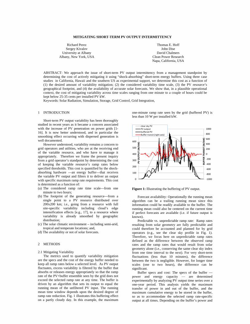
MITIGATING SHORT-TERM PV OUTPUT INTERMITTENCY Richard Perez Sergey Kivalov University at Albany Albany, New York, USA Thomas E. Hoff John Dise David Chalmers Clean Power Research Napa, California, USA ABSTRACT: We approach the issue of short-term PV output intermittency from a management standpoint by determining the cost of actively mitigating it using “shock-absorbing” short-term energy buffers. Using three case studies in California, Hawaii and the southern US as experimental support, we determine this cost as a function of (1) the desired amount of variability mitigation; (2) the considered variability time scale, (3) the PV resource’s geographical footprint, and (4) the availability of accurate solar forecasts. We show that, in a plausible operational context, the cost of mitigating variability across time scales ranging from one minute to a couple of hours could be kept below 25-35 cents per installed PV kW. Keywords: Solar Radiation, Simulation, Storage, Grid Control, Grid Integration, 1 INTRODUCTION Short-term PV output variability has been thoroughly studied in recent years as it became a concern associated with the increase of PV penetration on power grids [1- 16]. It is now better understood, and in particular the smoothing effect occurring with dispersed generation is well documented. However understood, variability remains a concern to grid operators and utilities, who are at the receiving end of the variable resource, and who have to manage it appropriately. Therefore we frame the present inquiry from a grid operator’s standpoint by determining the cost of keeping the variable resource’s ramp rates below specified thresholds. This cost is quantified by the shock- absorbing hardware —an energy buffer—that receives the variable PV output and filters it to deliver an output with specific maximum ramp rate requirements. This cost is determined as a function of: (a) The considered ramp rate time scale—from one minute to two hours; (b) The footprint of the generating resource—from a single point to a PV resource distributed over 200x200 km; i.e., going from a resource with full site-specific variability including cloud’s edge intensification effects [e.g., 17], to a resource where variability is already smoothed by geographic distribution; (c) The solar climatic environment – including semi-arid, tropical and temperate locations; and, (d) The availability or not of solar forecasts. 2 METHODS 2.1 Mitigating Variability The metrics used to quantify variability mitigation are the specs and the cost of the energy buffer needed to keep all ramp rates below a selected level. As PV output fluctuates, excess variability is filtered by the buffer that absorbs or releases energy appropriately so that the ramp rate of the PV+buffer ensemble seen by the grid does not exceed the selected ramp rate at any time. The buffer is driven by an algorithm that sets its output to equal the running mean of the unfiltered PV input. The running mean time window depends upon the desired degree of ramp rate reduction. Fig. 1 illustrates this buffering effect on a partly cloudy day. In this example, the maximum one-minute ramp rate seen by the grid (buffered PV) is less than 10 W per installed kW. ‐1000 ‐800 ‐600 ‐400 ‐200 0 200 400 600 800 1000 0 100 200 300 400 500 600 BUFFER TRANSIT (W/kW) PV OUTPUT (W/kW) clear sky PV PV output buffered PV Buffer transit (right axis) Figure 1: Illustrating the buffering of PV output. Forecast availability: Operationally the running mean algorithm can be a trailing running mean since this information could be readily available to the buffer. The running mean could also be centered on the current time if perfect forecasts are available (i.e. if future output is known). Predictable vs. unpredictable ramp rate: Ramp rates resulting from solar geometry are fully predictable and could therefore be accounted and planned for by grid operators (e.g., see the clear sky profile in Fig. 1). Therefore, we focus here on unpredictable ramp rates defined as the difference between the observed ramp rates and the ramp rates that would result from solar geometry alone (i.e., conserving the same clear sky index from one time interval to the next). For very short-term fluctuations (less than 10 minutes), the difference between the two is negligible. However, for longer time scales (one to two hours), the difference can be significant. Buffer specs and cost: The specs of the buffer — power and energy capacity — are determined experimentally by analyzing PV output time series over a one-year period. This analysis yields the maximum transfer of power in and out of the buffer, and the maximum cumulative energy to be stored in the buffer, so as to accommodate the selected ramp rate-specific output at all times. Depending on the buffer’s power and
Transcript
MITIGATING SHORT-TERM PV OUTPUT INTERMITTENCY
Richard Perez Sergey Kivalov
University at Albany Albany, New York, USA
Thomas E. Hoff John Dise
David Chalmers Clean Power Research Napa, California, USA
ABSTRACT: We approach the issue of short-term PV output intermittency from a management standpoint by determining the cost of actively mitigating it using “shock-absorbing” short-term energy buffers. Using three case studies in California, Hawaii and the southern US as experimental support, we determine this cost as a function of (1) the desired amount of variability mitigation; (2) the considered variability time scale, (3) the PV resource’s geographical footprint, and (4) the availability of accurate solar forecasts. We show that, in a plausible operational context, the cost of mitigating variability across time scales ranging from one minute to a couple of hours could be kept below 25-35 cents per installed PV kW. Keywords: Solar Radiation, Simulation, Storage, Grid Control, Grid Integration,
1 INTRODUCTION Short-term PV output variability has been thoroughly studied in recent years as it became a concern associated with the increase of PV penetration on power grids [1-16]. It is now better understood, and in particular the smoothing effect occurring with dispersed generation is well documented. However understood, variability remains a concern to grid operators and utilities, who are at the receiving end of the variable resource, and who have to manage it appropriately. Therefore we frame the present inquiry from a grid operator’s standpoint by determining the cost of keeping the variable resource’s ramp rates below specified thresholds. This cost is quantified by the shock-absorbing hardware —an energy buffer—that receives the variable PV output and filters it to deliver an output with specific maximum ramp rate requirements. This cost is determined as a function of: (a) The considered ramp rate time scale—from one
minute to two hours; (b) The footprint of the generating resource—from a
single point to a PV resource distributed over 200x200 km; i.e., going from a resource with full site-specific variability including cloud’s edge intensification effects [e.g., 17], to a resource where variability is already smoothed by geographic distribution;
(c) The solar climatic environment – including semi-arid, tropical and temperate locations; and,
(d) The availability or not of solar forecasts. 2 METHODS 2.1 Mitigating Variability The metrics used to quantify variability mitigation are the specs and the cost of the energy buffer needed to keep all ramp rates below a selected level. As PV output fluctuates, excess variability is filtered by the buffer that absorbs or releases energy appropriately so that the ramp rate of the PV+buffer ensemble seen by the grid does not exceed the selected ramp rate at any time. The buffer is driven by an algorithm that sets its output to equal the running mean of the unfiltered PV input. The running mean time window depends upon the desired degree of ramp rate reduction. Fig. 1 illustrates this buffering effect on a partly cloudy day. In this example, the maximum
one-minute ramp rate seen by the grid (buffered PV) is less than 10 W per installed kW.
Figure 1: Illustrating the buffering of PV output. Forecast availability: Operationally the running mean algorithm can be a trailing running mean since this information could be readily available to the buffer. The running mean could also be centered on the current time if perfect forecasts are available (i.e. if future output is known). Predictable vs. unpredictable ramp rate: Ramp rates resulting from solar geometry are fully predictable and could therefore be accounted and planned for by grid operators (e.g., see the clear sky profile in Fig. 1). Therefore, we focus here on unpredictable ramp rates defined as the difference between the observed ramp rates and the ramp rates that would result from solar geometry alone (i.e., conserving the same clear sky index from one time interval to the next). For very short-term fluctuations (less than 10 minutes), the difference between the two is negligible. However, for longer time scales (one to two hours), the difference can be significant. Buffer specs and cost: The specs of the buffer —power and energy capacity — are determined experimentally by analyzing PV output time series over a one-year period. This analysis yields the maximum transfer of power in and out of the buffer, and the maximum cumulative energy to be stored in the buffer, so as to accommodate the selected ramp rate-specific output at all times. Depending on the buffer’s power and
energy requirements, different technologies may be considered. Very small energy and high power requirements would be met by fly wheels or capacitors. As energy vs. power requirements augment, technologies would evolve toward supercapacitors and batteries. For this study, we built a simple “technology-agnostic” cost model based on current reported costs for state-of-the-art energy storage equipment. This cost model is illustrated in Fig. 2.
Figure 2: Buffer storage cost model [18] 2.2 Data Analysis The experimental data used to determine buffer specs consist of one-year PV output time series for horizontally-mounted PV systems operating in three climatically distinct locations: Hanford, in Central California, Goodwin Creek in the southeastern US, and Kaleola in Hawaii. For each location, a total of 78 PV output time series are analyzed encompassing 13 geographical footprints—from a single point, to 200x200 km integrated output—and 6 time scales —from one minute to two hours. One-minute PV output time series are simulated from one-minute high-resolution SolarAnywhere irradiances [19] in each 1x1 km high-resolution point in the considered 200x200 km regions (i.e., a total of ~ 40,000 points per region). These time series are averaged appropriately in space and in time to produce the desired time scales and footprints. The single-point PV output located at the center of each 200x200km region is simulated from actual irradiance measurements [20]. For any selected ramp rate reduction target and for each of the 78 space/time configurations, the buffer’s energy and power requirements as well as the running mean window are determined by calculating the difference between the running mean PV and the unfiltered PV output. The power requirements correspond to the highest absolute difference between the two, while the energy requirements correspond to the largest sum of accumulated differences while accounting for storage efficiency set at 95%. For each simulation, two types of running mean windows are considered: (1) trailing—no forecasts available, and (2) centered—ideal forecasts available. Trailing windows are extended as necessary to meet the maximum allowable ramp rate objectives. The lowest ramp rate objectives considered for this analysis are a function of the considered time scale, and range from 0.5% of installed capacity for one-minute fluctuations, to 10% for two-hour fluctuations.
2.3 Post-calibration of satellite data Because satellite-based simulations are derived from
irradiance models that are bound at the high end by clear sky, and at the low end by standard overcast conditions, they tend, at this stage of their development, to underestimate the dynamic range generated by highly variable conditions (e.g., see [10]). Short of producing a new satellite model with enhanced dynamics, we apply here post-calibration approach that ensures that simulation output discontinuities observed as a function of footprint from the single (measured) point to the extended (satellite) points are eliminated. This process is illustrated in Fig. 3 for one of the calculated variables: 15 minute PV output variability. The [underestimated] satellite-derived trend is adjusted upward so that it naturally converges to the (measured) single point without discontinuity. A similar post-result calibration is applied to all the simulated output variables including, in addition to variability, all the buffer specs—energy, power and cost —produced in the present analysis.
Figure 3: Illustration of the satellite data post-result calibration process. This example is shown for the 15-minute PV output variability observed in Hanford.
3 RESULTS
3.1 PV output variability Figs. 4 and 5 report respectively the PV output variability and maximum absolute ramps observed at each location as a function of time scale and geographic footprint. PV output variability is defined as the standard deviation of the ramps per Hoff and Perez, [16]. While these results are consistent with earlier findings by the authors and others [16] showing that variability decreases as a function of footprint at a rate that is dependent upon the considered time scale, they also show interesting site differences and similarities between locations: Variability increases as a function of time scale at all locations in the considered 1-minute to 2-hour domain, with an exception for Hawaii, where the trend is reversed for very small footprints. This is likely because of the frequent occurence of puffy cloud conditions resulting in high frequency variability at that site. As footprint increases beyond ~ 10 km, the trends are very similar for all sites, with highest overall values found for Goodwin Creek and lowest values found for Central California -- a likely results of the higher occurences of intermediate conditions in the Southeastern US compared to California and generally faster moving cloud systems inducing a
smaller decrease of variability with distance [2,12,16].
Figure 4: PV Output Variability (standard deviation of ramps) a Function of time scale and footprint When looking at maximum ramps as the metric for variability, the similarity observed between all sites is remarkable (see Fig. 5), particularly for small footprints where ramp values are almost identical for all sites at all time scales. For small footprints, highest values are observed for high frequency ramps, while this tendency is reversed -- highest values for low frequency ramps -- beyond 1-5 km footprint. 3.2 Mitigating variability – buffer specs Buffer specifications were determined for each of the 78 space/time configuration at each location. For each simulation, up to seven ramp mitigation targets and two forecast scenarios were considered. We present here a crosscut of these result that is representative of this work’s key findings, including:
(a) Influence of time scale, foot print and forecast availability for a given ramp rate mitigation objective; (b) Influence of ramp rate mitigation objective for selected footprints and time scales; and (c) Determination of buffer specs for a plausible operational objective.
Complete simulation results will be made available in a project report scheduled for publication at the end of 2013 [21].
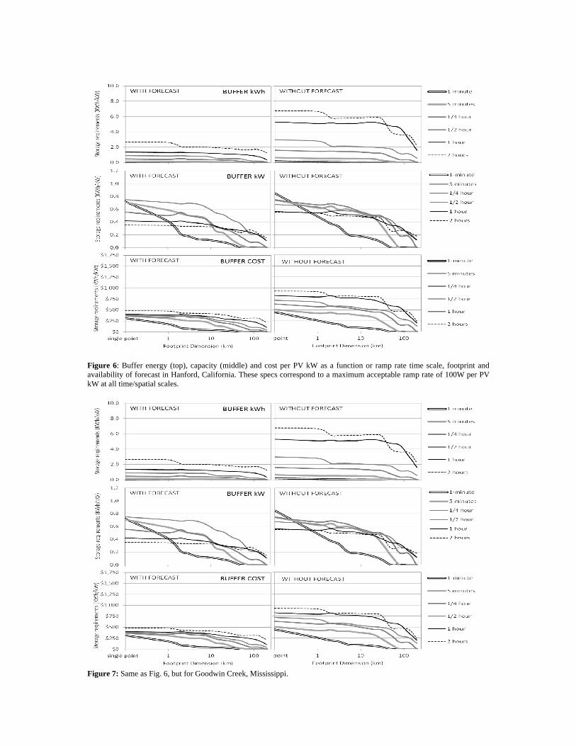
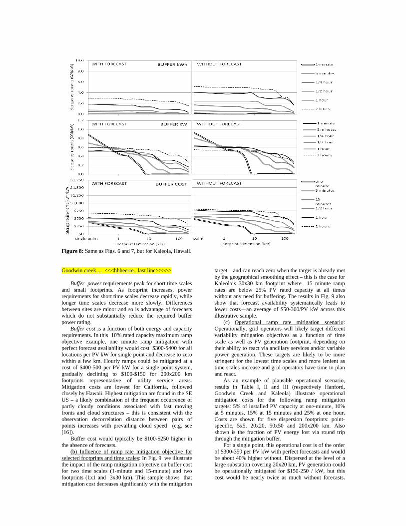
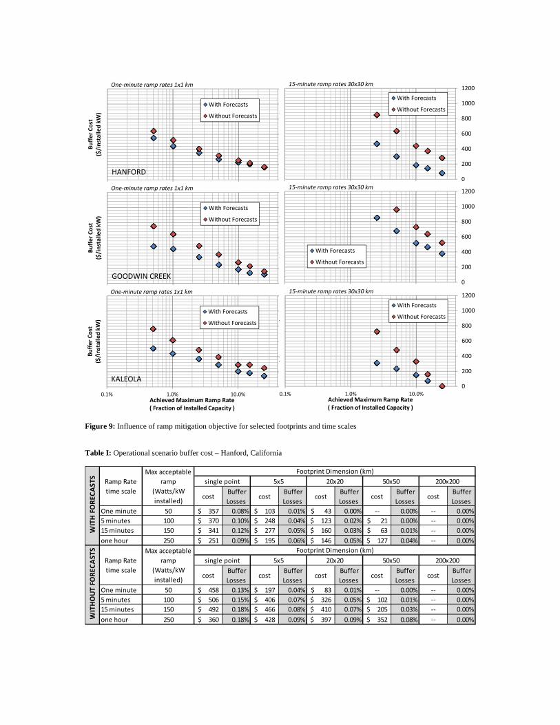
Figure 5: Maximum absolute ramp rate observed at ach location as a function of time scale and footprint. (a) Influence of time scale, foot print and forecast availability for a given ramp mitigation objective: The ramp obejective selected to illustrate the results is 100Watts per kW PV (i.e., 10% of installed capacity). For all considered time scales, footprints, locations and forecast scenarios, we present the buffer specification required to meet this maximum output ramp rate objective. Results are presented in Figs. 6, 7 and 8 for Hanford, Goodwin Creek and Kaleola, respectively. Buffer Energy requirements are primarily influenced by the considered time scale. Energy requirements are insignificant for short time scales and gradually increase with the considered time scale. The impact of footprint is also noticeable but not as pronounced, particularly for the longer time scales. The influence of forecast availability is noteworthy: energy requirements are markedly smaller when forecasts are available to drive the buffer’s running mean algorithm. This is particularly visible for the longer time frames, where the non-forecast trailing window must reach into the previous day’s conditions to meet the 100 W/kW maximum ramp rate objective presented in this example. Interestingly, the forecast advantage for longer time frames is more pronounced in California than it is in Hawaii. A possible explanation is that cloud conditions in Hawaii do not evolve as they do in California driven by the passing of fronts and cloud structures, but tend to remain comparable and repetitive over time, (i.e., the future is not as different from the past in Hawaii as it may be in California.)
Figure 6: Buffer energy (top), capacity (middle) and cost per PV kW as a function or ramp rate time scale, footprint and availability of forecast in Hanford, California. These specs correspond to a maximum acceptable ramp rate of 100W per PV kW at all time/spatial scales.
Figure 7: Same as Fig. 6, but for Goodwin Creek, Mississippi.
Figure 8: Same as Figs. 6 and 7, but for Kaleola, Hawaii. Goodwin creek.... <<<hhheerre.. last line>>>>> Buffer power requirements peak for short time scales and small footprints. As footprint increases, power requirements for short time scales decrease rapidly, while longer time scales decrease more slowly. Differences between sites are minor and so is advantage of forecasts which do not substantially reduce the required buffer power rating. Buffer cost is a function of both energy and capacity requirements. In this 10% rated capacity maximum ramp objective example, one minute ramp mitigation with perfect forecast availability would cost $300-$400 for all locations per PV kW for single point and decrease to zero within a few km. Hourly ramps could be mitigated at a cost of $400-500 per PV kW for a single point system, gradually declining to $100-$150 for 200x200 km footprints representative of utility service areas. Mitigation costs are lowest for California, followed closely by Hawaii. Highest mitigation are found in the SE US – a likely combination of the frequent occurrence of partly cloudy conditions associated with fast moving fronts and cloud structures – this is consistent with the observation decorrelation distance between pairs of points increases with prevailing cloud speed (e.g. see [16]). Buffer cost would typically be $100-$250 higher in the absence of forecasts. (b) Influence of ramp rate mitigation objective for selected footprints and time scales: In Fig. 9 we illustrate the impact of the ramp mitigation objective on buffer cost for two time scales (1-minute and 15-minute) and two footprints (1x1 and 3x30 km). This sample shows that mitigation cost decreases significantly with the mitigation
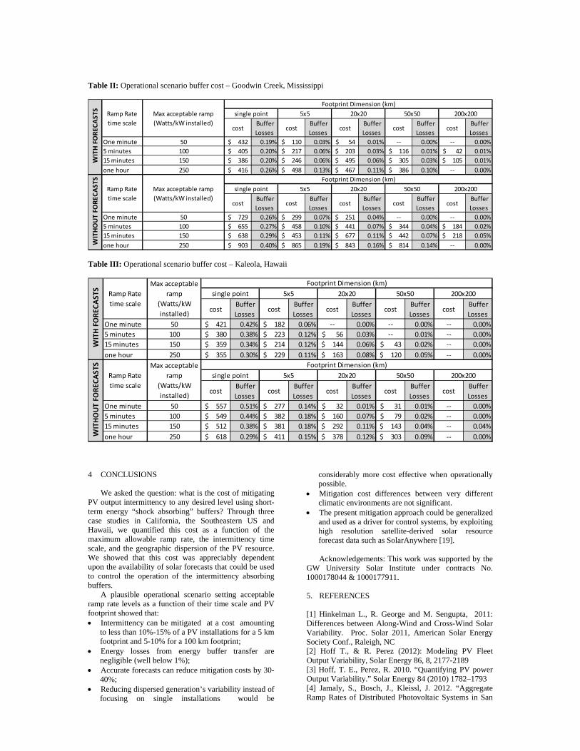
target—and can reach zero when the target is already met by the geographical smoothing effect – this is the case for Kaleola’s 30x30 km footprint where 15 minute ramp rates are below 25% PV rated capacity at all times without any need for buffering. The results in Fig. 9 also show that forecast availability systematically leads to lower costs—an average of $50-300/PV kW across this illustrative sample. (c) Operational ramp rate mitigation scenario: Operationally, grid operators will likely target different variability mitigation objectives as a function of time scale as well as PV generation footprint, depending on their ability to react via ancillary services and/or variable power generation. These targets are likely to be more stringent for the lowest time scales and more lenient as time scales increase and grid operators have time to plan and react. As an example of plausible operational scenario, results in Table I, II and III (respectively Hanford, Goodwin Creek and Kaleola) illustrate operational mitigation costs for the following ramp mitigation targets: 5% of installed PV capacity at one-minute, 10% at 5 minutes, 15% at 15 minutes and 25% at one hour. Costs are shown for five dispersion footprints: point-specific, 5x5, 20x20, 50x50 and 200x200 km. Also shown is the fraction of PV energy lost via round trip through the mitigation buffer. For a single point, this operational cost is of the order of $300-350 per PV kW with perfect forecasts and would be about 40% higher without. Dispersed at the level of a large substation covering 20x20 km, PV generation could be operationally mitigated for $150-250 / kW, but this cost would be nearly twice as much without forecasts.
0
200
400
600
800
1000
1200
0.1% 1.0% 10.0%
Buffer Cost
($/installed kW)
Achieved Maximum Ramp Rate( Fraction of Installed Capacity )
With Forecasts
Without Forecasts
One‐minute ramp rates 1x1 km
0
200
400
600
800
1000
1200
0.1% 1.0% 10.0%
()
Achieved Maximum Ramp Rate( Fraction of Installed Capacity )
With Forecasts
Without Forecasts
15‐minute ramp rates 30x30 km
0
200
400
600
800
1000
1200
0.1% 1.0% 10.0%
Buffer Cost
($/installed kW)
Achieved Maximum Ramp Rate( Fraction of Installed Capacity )
With Forecasts
Without Forecasts
One‐minute ramp rates 1x1 km
0
200
400
600
800
1000
1200
0.1% 1.0% 10.0%
(/
)
Achieved Maximum Ramp Rate( Fraction of Installed Capacity )
With Forecasts
Without Forecasts
15‐minute ramp rates 30x30 km
HANFORD
GOODWIN CREEK
KALEOLA
Figure 9: Influence of ramp mitigation objective for selected footprints and time scales Table I: Operational scenario buffer cost – Hanford, California
one hour 250 618$ 0.29% 411$ 0.15% 378$ 0.12% 303$ 0.09% ‐‐ 0.00% WITHOUT FORECASTS
W
ITH FOREC
ASTS
Footprint Dimension (km)
single point
5x5 20x20 50x50 200x200
5x5 20x20 50x50 200x200
Footprint Dimension (km)
single pointRamp Rate
time scale
Max acceptable
ramp
(Watts/kW
installed)
Ramp Rate
time scale
Max acceptable
ramp
(Watts/kW
installed)
4 CONCLUSIONS
We asked the question: what is the cost of mitigating PV output intermittency to any desired level using short-term energy “shock absorbing” buffers? Through three case studies in California, the Southeastern US and Hawaii, we quantified this cost as a function of the maximum allowable ramp rate, the intermittency time scale, and the geographic dispersion of the PV resource. We showed that this cost was appreciably dependent upon the availability of solar forecasts that could be used to control the operation of the intermittency absorbing buffers. A plausible operational scenario setting acceptable ramp rate levels as a function of their time scale and PV footprint showed that: Intermittency can be mitigated at a cost amounting
to less than 10%-15% of a PV installations for a 5 km footprint and 5-10% for a 100 km footprint;
Energy losses from energy buffer transfer are negligible (well below 1%);
Accurate forecasts can reduce mitigation costs by 30-40%;
Reducing dispersed generation’s variability instead of focusing on single installations would be
considerably more cost effective when operationally possible.
Mitigation cost differences between very different climatic environments are not significant.
The present mitigation approach could be generalized and used as a driver for control systems, by exploiting high resolution satellite-derived solar resource forecast data such as SolarAnywhere [19].
Acknowledgements: This work was supported by the GW University Solar Institute under contracts No. 1000178044 & 1000177911. 5. REFERENCES [1] Hinkelman L., R. George and M. Sengupta, 2011: Differences between Along-Wind and Cross-Wind Solar Variability. Proc. Solar 2011, American Solar Energy Society Conf., Raleigh, NC [2] Hoff T., & R. Perez (2012): Modeling PV Fleet Output Variability, Solar Energy 86, 8, 2177-2189 [3] Hoff, T. E., Perez, R. 2010. “Quantifying PV power Output Variability.” Solar Energy 84 (2010) 1782–1793 [4] Jamaly, S., Bosch, J., Kleissl, J. 2012. “Aggregate Ramp Rates of Distributed Photovoltaic Systems in San
Diego County.” IEEE Transactions on Sustainable Energy, in press [5] Lave, M., J. Kleissl, Arias-Castro, E., High-frequency fluctuations in clear-sky index, Solar Energy, doi:10.1016/j.solener.2011.06.031, 2011 [6] Lorenz E., T. Scheidsteger, J. Hurka, D. Heinemann and C. Kurz, (2011): Regional PV power prediction for improved grid integration. Progress in Photovoltaics, 19, 7, 757-771. [7] Mills, A., Wiser, R. 2010. Implications of Wide-Area Geographic Diversity for Short-Term Variability of Solar Power. Lawrence Berkeley National Laboratory Technical Report LBNL-3884E. [8] Murata, A., H. Yamaguchi, and K. Otani (2009): A Method of Estimating the Output Fluctuation of Many Photovoltaic Power Generation Systems Dispersed in a Wide Area, Electrical Engineering in Japan, Volume 166, No. 4, pp. 9-19 [9] Perez M., and V. Fthenakis, (2012): Quantifying Long Time Scale Solar Resource Variability. Proc. WREF, Denver, CO. [10] Perez, R., T. Hoff and S. Kivalov, (2011a): Spatial & temporal characteristics of solar radiation variability. Proc. of International Solar Energy (ISES) World Congress, Kassel, Germany [11] Perez, R., Kivalov, S., Schlemmer, J., Hemker Jr., C. , Hoff, T. E. (2011b): Parameterization of site-specific short-term irradiance variability, Solar Energy 85 (2011) 1343-1353 [12] Perez, R., Kivalov, S., Schlemmer, J., Hemker Jr., C. , Hoff, T. E. (2012): “Short-term irradiance variability correlation as a function of distance.” Solar Energy 86, 8,
pp. 2170-2176 [13] Wiemken E., H. G. Beyer, W. Heydenreich and K. Kiefer (2001): Power Characteristics of PV ensembles: Experience from the combined power productivity of 100 grid-connected systems distributed over Germany. Solar Energy 70, 513-519 [14] Woyte, A., Belmans, R., Nijs, J. (2007): Fluctuations in instantaneous clearness index. Solar Energy 81 (2), 195-206. [15] Marcos J., L. Morroyo, E. Lorenzo and M. Garcia, (2012): Smoothing of PV power fluctuations by geographical dispersion. Prog. Photovolt: Res. Appl. 2012; 20:226–237 [16] Perez, R., T. Hoff, (2013): Solar Resource Variability, in: Solar Resource Assessment & Forecasting (Ed. J. Kleissl), Elsevier, 2013 [17] Yordanov, G., O. Mitdgard, O. and L. Norum (2013): Overirradiance (Cloud Enhancement) Events at High Latitudes. IEEE Journal of Photovoltaics, 3, 1, 271-278. [18] Germa, J.M., & M. Perez, (2012): Energy Storage: Technology, Applications & trends. Cluster Maritime Français. 10/3/12 [19] SolarAnywhere (2013): http://www.cleanpower.com/products/solaranywhere/solaranywhere-data / [20] NOAA SURFRAD & ISIS Networks: http://www.esrl.noaa.gov [21] Perez R. and T. Hoff (2013): Final Report on PV Variability Mitigation. GW University Report on contract No. under contracts No. 1000178044 (in preparation)


![Simulation of Atmospheric Wave-Fronts with Turbulence ... · turbulence, the so called intermittency [16] [17]. The intermittency is assumed usually stationary, isotropic, h o-mogeneous,](https://static.documents.pub/doc/80x56/5eb236ead5f7df0fcf1e5114/simulation-of-atmospheric-wave-fronts-with-turbulence-turbulence-the-so-called.jpg)


