9 Mixed Membership Trajectory Models Daniel Manrique-Vallier Department of Statistics, Indiana University, Bloomington, IN 47408, USA CONTENTS 9.1 Introduction ................................................................................ 173 9.1.1 Application: The National Long Term Care Survey ................................. 174 9.2 Longitudinal Trajectory Models ............................................................ 176 9.2.1 Clustering Based on Trajectories .................................................... 176 9.2.2 Hard Clustering: Group-Based Trajectory Models ................................... 176 9.2.3 Soft Clustering: The Trajectory GoM model ........................................ 177 9.2.4 Latent Class Representation of the TGoM ........................................... 179 9.2.5 Specifying the Trajectory Function .................................................. 180 9.2.6 Completing the Specification ....................................................... 180 9.3 Estimation through Markov Chain Monte Carlo Sampling ................................... 181 9.3.1 Tuning the Population Proposal Distribution ........................................ 183 9.4 Using the TGoM ........................................................................... 184 9.5 Discussion and Extensions .................................................................. 187 References ................................................................................. 187 We present a model in which individuals can have multiple membership into “pure types” defined by ways of evolving over time. This modeling strategy allows us to use longitudinal data on several subjects to isolate and characterize a few typical trajectories over time, and to soft cluster individuals with respect to them. We present these methods in the context of an application to the study of patterns of aging in American seniors. 9.1 Introduction In this chapter we introduce a Bayesian technique for soft clustering units based on similarities on their temporal evolution using longitudinal data. Clustering based on evolution over time, or tra- jectories, is of interest in many areas. For example, criminology researchers are often interested in identifying types of “criminal careers,” and in determining how a population of offenders distributes across them (Nagin and Land, 1993). Similarly, clinical psychologists might be interested in char- acterizing the developmental course of specific disorders like depression (Dekker et al., 2007) or post-traumatic stress disorder (Orcutt et al., 2004). In general terms, the typical clustering problem consists of arranging a number of units, e.g., a sample of people, into a smaller number of classes based on the similarity of some observed attributes without assuming prior knowledge of the specific characteristics of the groups. From a 173
Transcript
9Mixed Membership Trajectory Models
Daniel Manrique-VallierDepartment of Statistics, Indiana University, Bloomington, IN 47408, USA
We present a model in which individuals can have multiple membership into “pure types” definedby ways of evolving over time. This modeling strategy allows us to use longitudinal data on severalsubjects to isolate and characterize a few typical trajectories over time, and to soft cluster individualswith respect to them. We present these methods in the context of an application to the study ofpatterns of aging in American seniors.
9.1 Introduction
In this chapter we introduce a Bayesian technique for soft clustering units based on similarities ontheir temporal evolution using longitudinal data. Clustering based on evolution over time, or tra-jectories, is of interest in many areas. For example, criminology researchers are often interested inidentifying types of “criminal careers,” and in determining how a population of offenders distributesacross them (Nagin and Land, 1993). Similarly, clinical psychologists might be interested in char-acterizing the developmental course of specific disorders like depression (Dekker et al., 2007) orpost-traumatic stress disorder (Orcutt et al., 2004).
In general terms, the typical clustering problem consists of arranging a number of units, e.g.,a sample of people, into a smaller number of classes based on the similarity of some observedattributes without assuming prior knowledge of the specific characteristics of the groups. From a
173
174 Handbook of Mixed Membership Models and Its Applications
model-based perspective, this is usually accomplished by fitting mixtures of the form
p(y|π) =
K∑k=1
πkfk(y) (9.1)
to multivariate data about one or more individual characteristics, say y = (y1, ..., yJ), that are ex-pected to inform about the relevant differences between individuals. Models of this form are usuallyinterpreted as partitioning the population into K disjoint sub-populations, each representing a frac-tion πk of the population. The sub-populations themselves are characterized by (usually parametric)densities fk(), which are also to be estimated from the data.
When dealing with phenomena that evolve over time it is occasionally of interest to cluster in-dividuals based on similarities on their temporal evolution. This requires longitudinal data, i.e.,repeated observations of the same individuals at different points in time. The most direct approachis to assume that there exists a number of sub-populations, each characterized by a particular tra-jectory, and that each individual belongs to one and only one of them. Such a setup correspondsto the general model-based clustering approach described in the previous paragraph. In particular,trajectories define specific forms of fk(), the sub-population’s joint distribution of the sequence ofobservations.
In some applications the requirement that each individual belong exclusively to just one sub-population can be too restrictive to be realistic. For example, in the study of political ideologyit is common to use terms that describe pure extreme positions, like “liberal” or “conservative.”However, actually assuming that every individual is either a liberal or a conservative is too broada description to be useful, let alone accurate. In particular, it hides the fact that many individualshave opinions about different topics that correspond to more than one “pure” ideological position.A better alternative would be to describe individuals’ ideologies as mixtures of the pure types.
Modeling these structures motivates the mixed membership approach. Mixed membership mod-els relax the assumption of exclusive cluster membership by allowing units to belong to more thanone group simultaneously. We call this type of arrangement a soft clustering.
In this chapter we extend the mixed membership approach to longitudinal structures based ontrajectories. In particular, our technique allows us to construct soft-classifications based on theways in which individuals evolve over time. This, in turn, allows us to isolate a few extreme orpure trajectories—which can be informative and easy to analyze—and to characterize units in thepopulation as individually-mixed combinations of them. We introduce this approach in the contextof studying the individual patterns of evolution of disability in the elder American population. Inthe next section we present the applied context, which will serve as our illustrative application.Then we introduce the general notion of clustering based on trajectories, and present our method,the Trajectory Grade of Membership model, as a mixed membership extension of this idea. Wepresent a fully Bayesian specification and an estimation algorithm based on Markov chain MonteCarlo (MCMC) sampling. Finally, we demonstrate the method by analyzing patterns of evolutionof disability using data from the National Long Term Care Survey. Additional details regarding themodel and analysis can be found in Manrique-Vallier (2013; 2010)
9.1.1 Application: The National Long Term Care Survey
It is well known that elder Americans are living longer than in the past. Their absolute number andproportion are increasing rapidly (Connor, 2006). Older people often require some form of long-term care, especially in the presence of disabilities (Manton et al., 1997). Thus, efficient allocationof resources and overall cost prediction require information about typical patterns of disability, theirprogression over time, and their distribution over the population.
With these issues in mind, a group of researchers and policy makers created the National LongTerm Care Survey, NLTCS (Clark, 1998). The NLTCS is a longitudinal survey designed to evaluate
Mixed Membership Trajectory Models 175
the state and progression of chronic disability among the senior population in the United States. Thisinstrument tracks disability by recording each individual’s capacity to perform a set of “Activitiesof Daily Living” (ADL) such as eating, bathing, or dressing, and “Instrumental Activities of DailyLiving” (IADL) such as preparing meals or maintaining finances.
The NLTCS is comprised of six waves of interviews, administered in 1982, 1984, 1989, 1994,1999, and 2004. Each wave includes interviews of about 20,000 people. Whenever possible, indi-viduals are followed from wave to wave until death. However, due to the high mortality rate in thetarget population, each wave also includes a replacement sample of approximately 5,000 new sub-jects. The inclusion of these new individuals keeps each wave’s sample size approximately constantand representative of the population at each given time (Clark, 1998). In aggregate, approximately49,000 people have been interviewed between 1982 and 2004.
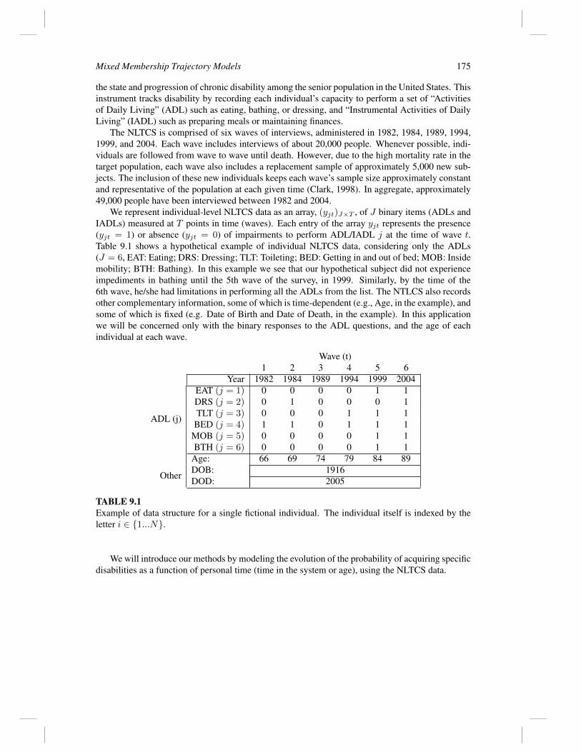
We represent individual-level NLTCS data as an array, (yjt)J×T , of J binary items (ADLs andIADLs) measured at T points in time (waves). Each entry of the array yjt represents the presence(yjt = 1) or absence (yjt = 0) of impairments to perform ADL/IADL j at the time of wave t.Table 9.1 shows a hypothetical example of individual NLTCS data, considering only the ADLs(J = 6, EAT: Eating; DRS: Dressing; TLT: Toileting; BED: Getting in and out of bed; MOB: Insidemobility; BTH: Bathing). In this example we see that our hypothetical subject did not experienceimpediments in bathing until the 5th wave of the survey, in 1999. Similarly, by the time of the6th wave, he/she had limitations in performing all the ADLs from the list. The NTLCS also recordsother complementary information, some of which is time-dependent (e.g., Age, in the example), andsome of which is fixed (e.g. Date of Birth and Date of Death, in the example). In this applicationwe will be concerned only with the binary responses to the ADL questions, and the age of eachindividual at each wave.
TABLE 9.1Example of data structure for a single fictional individual. The individual itself is indexed by theletter i ∈ {1...N}.
We will introduce our methods by modeling the evolution of the probability of acquiring specificdisabilities as a function of personal time (time in the system or age), using the NLTCS data.
176 Handbook of Mixed Membership Models and Its Applications
9.2 Longitudinal Trajectory Models9.2.1 Clustering Based on Trajectories
Multivariate data arising from longitudinal studies can sometimes be thought of as the expressionof a time-continuous underlying process. For example, in the study of disability among elders, itis reasonable to assume that the sequence of discrete disability measurements of an individual isan observable expression of an underlying “aging process,” that relates age to the probability ofexperiencing a disability. We can go further and assume that this process is such that the probabilityof experimenting a functional disability will tend to increase as the person ages.
In some applications it is possible to describe the evolutionary process that underlies the ob-served longitudinal data using parametric functions of time or of a time-dependent covariate. Wecall these functions trajectories. An example of a trajectory is a function of age that determines theprobability of experimenting a disability.
When the population under study is, or may be expected to be, heterogeneous, we cannot assumethat every individual in the population follows the same underlying trajectory. In our application,for example, that would force us to expect that all individuals age the same way. Instead, whenmodeling these situations, we need to allow distinct individuals to respond to different trajectories.
Adopting such a modeling scheme, where each individual is allowed to have his/her own trajec-tory, opens up the possibility of clustering the population based on similarities among trajectories.For instance we could try to cluster individuals from the NLTCS into classes defined by “types ofaging.” We call this clustering strategy clustering based on trajectories. Besides its intrinsic ap-plication domain interest, clustering based on trajectories has also the advantage of allowing us toincorporate additional knowledge about the trajectories (e.g., their expected shape) to complementthe information already contained in the individual sequences of responses.
9.2.2 Hard Clustering: Group-Based Trajectory Models
A direct approach to clustering based on trajectories is given by group-based trajectory models(GBTM) (Nagin, 1999; Connor, 2006). These models assume the existence of a few homogeneoussub-populations whose members’ responses follow the same trajectories over time. Thus, it enablesa type of hard-clustering of the population of interest.
To see how a GBTM works, let us consider modeling the progression of a single binary response.Let y = (y1, ..., yt, ..., yT ) be the sequence of binary measurements at times t = 1, 2, ..., T for thesame individual. We assume that the individual has been sampled from one of K sub-populations,with probability πk (k = 1, 2, ...,K). Then we specify the trajectory of the probability of a positiveresponse for a member of group k, Φθk(x) as some convenient function of a time-varying quantityx, indexed by parameters θk:
Φθk(x) = Pr(yt = 1|x, individual belongs to group k).
Let x = (x1, x2, ..., xT ) be a vector containing the T measurements of the time-dependentquantity of interest, e.g., the age of the individual at each survey wave. Then, assuming that givengroup membership and xt, responses are all independent, we have that
p(y|x, θ) =
K∑k=1
πk
T∏t=1
fθk(yt;xt), (9.2)
where fθk(yt|x) = Φθk(x)yt(1 − Φθk(x))1−yt . The model in (9.2) is a discrete mixture thatspecifies the distribution of a response variable within each sub-population, conditional on a time-dependent covariate.
Mixed Membership Trajectory Models 177
Connor (2006) proposed an extension for multivariate binary data consisting of J binary vari-ables measured at T points in time, and applied it to the analysis of the NLTCS. His proposalextended (9.2) by assuming conditional independence between responses to different items at dis-tinct points in time, given covariates and group membership. Let yjt be the response to item j atmeasurement t (e.g., to the jth ADL of the NLTCS at wave t). Connor’s model is
p(y|x, θ) =
K∑k=1
πk
J∏j=1
T∏t=1
fθjk(yjt;xt). (9.3)
This specification characterizes each sub-population based on J trajectories, each of them commonto all of their members.
9.2.3 Soft Clustering: The Trajectory GoM model
The requirement of group-based GBTM of within-cluster homogeneity can be too restrictive insome applications. For instance, in the NLTCS case it essentially requires us to assume that everyindividual within a sub-population follows the exact same aging process. This is not plausible.Furthermore, one might even wonder if such sub-populations exist at all (see e.g., Kreuter andMuthen, 2008).
One way of relaxing this strong assumption is by replacing the requirement of exclusive mem-bership with a mixed membership structure—thus constructing a soft clustering based on trajec-tories. In such a case, we interpret latent groups not as sub-populations—as with group-basedtrajectory models—but as characterizations of extreme cases. We then model individual trajectoriesas mixtures of extreme trajectories in different individual degrees.
The rest of this section is devoted to presenting one such model, which we will call a TrajectoryGrade of Membership (TGoM) model.
In longitudinal multivariate settings we are interested in studying the simultaneous progressionof a number, J , of variables as a function of time. For now, assume that response variables arebinary and that we have measurements of each variable at a number, T , of points in time. Call yjtthe value of the jth variable (j = 1, ..., J) at measurement time t (t = 1, ..., T ) for a particularindividual. In the NLTCS case, yjt is the disability measurement j (jth ADL) at wave t.
Similar to a group-based trajectory model, we assume the existence of a small number, K, ofideal types of individuals or extreme profiles. However, instead of assuming that particular individ-uals belong completely to those classes, we endow them with membership vectors, g = (g1..., gK)(gk > 0,
∑k gk = 1). Membership vectors are a characteristic of each individual. Their compo-
nents, gk, represent the degree of membership of an individual in each of the K extreme profiles.Ideal individuals of the kth type are individuals whose membership vector’s kth component has avalue gk = 1, and the rest of the entries are zeros. For instance, an individual with membershipvector g = (0, 1, 0, 0) belongs exclusively to the extreme profile k = 2. An individual with mem-bership vector g = (0.1, 0.2, 0.7) has 10% membership in extreme profile k = 1, 20% in k = 2,and 70% in k = 3.
We specify the trajectory of a positive response for each response variable j and extreme profilek, Φθjk(x) as a function of time with parameter θjk. These trajectories correspond to idealized pro-gressions of the variables of interest over time, in the same way that trajectories in the developmen-tal trajectory model represent the progression of variables for particular groups over time. Differentfrom GBTM though, we do not regard individuals as being samples from the sub-population, butmixtures of them.
Using the membership vectors, we model the trajectory of variable j for an individual with
178 Handbook of Mixed Membership Models and Its Applications
65 70 75 80 85 90
0.0
0.2
0.4
0.6
0.8
1.0
x
Pro
babi
lity
k = 1k = 2k = 3
FIGURE 9.1Example of extreme and individual trajectories. Extreme trajectories are drawn in thick lines. In-dividuals have membership vectors (0.1, 0.2, 0.7) (top thin solid curve) and (0.2, 0.7, 0.1) (bottomthin solid curve).
membership vector g = (g1, ..., gK) as
p (yjt |(g1, ..., gK), x, θ ) =
K∑k=1
gkfθjk(yjt;x). (9.4)
As an example with K = 3 extreme profiles, consider the situation in Figure 9.1. Curves in thicklines represent three extreme trajectories, Φθj1(x), Φθj2(x), Φθj3(x), for an arbitrary ADL, j. Ac-cording to (9.4), given an individual i whose membership vector is gi, the probability of a positiveresponse to item j is a weighted combination of the extremes, which defines an individualizedtrajectory, Φ(i)(x) = Pr(yij = 1|gi, x) =
correspond to (most likely fictional) individuals whose membership vectors are (1, 0, 0), (0, 1, 0),and (0, 0, 1). The two individual trajectories—thin lines—in the picture correspond to individualswhose membership vectors are (0.1,0.2,0.7) and (0.2, 0.7, 0.1).
In order to characterize the joint distribution of individual responses, we introduce a local inde-pendence assumption: for a single individual, conditional on the value of the covariate of interest attime t, xt, and its membership vector, g, the J responses at each of the T measurement times aremutually independent:
p (y |(g1, ..., gK), (x1, ..., xT ), θ ) =
J∏j=1
T∏t=1
K∑k=1
gkfθjk(yjt;xt). (9.5)
Moving to the sample, we assume that there are N individuals. We index them using the letteri = 1, . . . , N and add a corresponding sub-index to the individual-level quantities yi, gi, and xi.Assuming that each individual has been randomly sampled from the population, we get the jointmodel for the whole sample y, conditional on all the membership vectors g, and all the time-varying
Mixed Membership Trajectory Models 179
covariates x:
p (y |g,x, θ ) =
N∏i=1
J∏j=1
T∏t=1
K∑k=1
gikfθjk(yijt;xit). (9.6)
Finally, assuming that the membership vectors are i.i.d. samples from a common distribution, sayFα, we get the model
p (y|x,g, θ) =
N∏i=1
∫∆
J∏j=1
T∏t=1
K∑k=1
gkfθjk(yijt;xit)Fα(dg). (9.7)
9.2.4 Latent Class Representation of the TGoM
Similar to the Grade of Memberhsip model (see Erosheva et al., 2007), the model in (9.5) admits anaugmented data representation that makes it similar to the group-based multivariate developmentaltrajectory model in (9.3). A few algebraic manipulations on (9.5) (Erosheva, 2002) lead to theequivalence
J∏j=1
T∏t=1
K∑k=1
gkfθjk(yjt;xt) =∑z∈Z
J∏j=1
T∏t=1
gzjfθjzjt (yjt;xt), (9.8)
where Z = {1, 2, ...,K}J×T is the set of all matrices (zjt) whose entries take values in{1, 2, ...,K}. From here it follows that, after summing over all possible realizations of z, the model
p (y, z |x, θ, g ) =
J∏j=1
T∏t=1
K∏k=1
[gkfθjk(yjl;xt)
]I(zjt=k)
(9.9)
is equivalent to (9.5). For details applied to the case of the GoM model, see Erosheva et al. (2007).Considering that g ∼ G and integrating (9.9), we get the unconditional distribution
p (y|x) =∑z∈Z
πz
J∏j=1
T∏t=1
fθjk(yjt;xt), (9.10)
where
πz = EG
J∏j=1
T∏t=1
K∏k=1
gI(zjt=k)k
. (9.11)
Equation (9.10) shows that the TGoM can be seen as a multivariate group-based DTM, just like(9.3), where the membership weights are restricted by the moments-based definition of πz in (9.11).We can also see that the following generative process will produce N multivariate responses ac-cording to (9.10). Here we again add the individual index, i ∈ {1, ..., N}, to yjt, g, and zjt.
180 Handbook of Mixed Membership Models and Its Applications
Trajectory GoM Individual Response Generation Process
In our application it is reasonable to assume that the probability of presenting a disability shouldincrease monotonically with age. We thus follow Connor (2006) in making θjk = (β0jk, β1jk) andusing the s-shaped function
Φθjk(x) =1
1 + exp(−β0jk − β1jkx), (9.12)
where x is a scalar representing age.In general, the choice of trajectory functions Φjk(·) must be application-specific, as they encode
assumptions about the nature of the underlying process. Thus, other applications would likelyrequire different specifications.
9.2.6 Completing the Specification
To complete a full Bayesian specification of the TGoM model, we need to specify the membershipdistribution Fα and prior distributions for its parameter α and for the trajectory parameters θjk.
Following Erosheva et al. (2007), we assume gi|α ∼ Dirichlet(α), where α = (α0 · ξ1, α0 ·ξ2, ..., α0 · ξK) with α0 and ξk > 0 for all k = 1, 2, ...,K, and
∑Kk=1 ξk = 1. Under this
parametrization, ξ = (ξ1, ..., ξK) is the expected value of the distribution. It also, more informally,represents the relative importance of profile k in the population. In turn, α0 is a concentration pa-rameter: the closer α0 is to 0, the closer samples from Fα will be to the extreme profiles; conversely,the higher the value of α0, the closer the samples from Fα will tend to be to their expected value,ξ. Thus, for ξ fixed, α0 controls the amount of mixed membership. We also follow Erosheva et al.(2007) in specifying independent prior distributions α0 ∼ Gamma(τ, η) and ξ ∼ Dirichlet(1K).
Other specifications are possible, and in some problems they may be necessary. An importantlimitation of the Dirichlet distribution is its simple correlation structure. Regular Dirichlet distri-butions do not allow the capture of complex correlations between membership in different extremeprofiles. This might be a limitation in applications where membership in some extreme profiles hasnon-trivial relationships with membership in other profiles. A natural extension that can be usefulin such situations is the multinomial logistic normal prior (see e.g., Blei and Lafferty, 2007). Unfor-tunately this specification does not share the computational advantages of the Dirichlet distribution.In particular, it is not conjugate to the multinomial distribution. For the parameters of the extremetrajectories specified in (9.12), β, we specify independent prior distributions β0jk
iid∼ N(µβ0, σ2β0)
and β1jkiid∼ N(µβ1 , σ
2β1).
Mixed Membership Trajectory Models 181
9.3 Estimation through Markov Chain Monte Carlo SamplingUnder the specification of extreme trajectories and priors outlined in this section, and following theaugmented data representation in (9.9), the joint posterior distribution of parameters and augmenteddata is
p(α, β, z,g|Data) ∝p(β)p(α)
(N∏i=1
p (gi|α)
)
×N∏i=1
J∏j=1
T∏t=1
K∏k=1
(gik
exp(yijtβ0jk + yijtβ1jkxit)
1 + exp(β0jk + β1jkxit)
)I(zijt=k)
.
Using the full Bayesian specification from Section 9.2.6 we have that
p(gi|α) = Dirichlet(gi|α1, α2, ..., αk),
p(α0) = Gamma(α0|τ, η),
p(ξ) = Dirichlet(ξ|1K
)(Uniform on the ∆K−1),
with p(α) = p(α0)·p(ξ), where α0 =∑k αk and ξ = (ξ1, ξ2, ..., ξK) with αk = α0·ξk. Parameters
τ and η are shape and inverse scale parameters, respectively.Specifying an MCMC algorithm to obtain approximate realizations from this posterior distribu-
tion using the Gibbs sampling algorithm is just a matter of obtaining the full conditional distributionsof each parameter and augmented data. An implementation of this algorithm follows.
1. Sampling from z: For every i ∈ {1 . . . N}, j ∈ {1 . . . J}, and t ∈ {1 . . . T}, sample
zijt|... ∼Discrete(p1, p2, ..., pK),
with pk ∝ gik exp(β0jk + β1jkxit)yijt [1 + exp(β0jk + β1jkxit)]
−1, for all k ∈ {1, . . . ,K}.
2. Sampling from (β0jk, β1jk): Let ρit = I(zijt = k). Then, the full joint conditional distributionof (β0jk, β1jk) is
p (β0jk, β1jk|...)
∝exp
[−β0jk
2
2σ02 + β0jk
(µ0
σ0+∑i,t
ρityijt
)− β1jk
2
2σ12 + β1jk
(µ1
σ1+∑i,t
ρitxityijt
)]∏i,t
[1 + exp (β0jk + β0jkxit)]ρit .
This distribution does not have a recognizable form. Thus we use a random walk Metropolisstep:
(a) Proposal step: Sample the proposal values
β∗0jk ∼ N(β0jk, σ2β0) and β∗1jk ∼ N(β1jk, σ
2β1),
where the values σ2β0 and σ2
β1 are tuning parameters that we have to calibrate to achievea good balance between acceptance of proposed values and exploration of the support ofthe target distribution.
182 Handbook of Mixed Membership Models and Its Applications
(b) Acceptance step: Compute
rM =p(β∗0jk, β
∗1jk|...)
p(β0jk, β1jk|...)
=∏i,t
1 + exp [β0jk + β0jkxit]
1 + exp[β∗0jk + β∗0jkxit
]ρit (9.13)
× exp
−β∗20jk − β20jk
2σ20
+(β∗0jk − β0jk
)µ0
σ0+∑i,t
ρityijt
× exp
−β∗21jk − β21jk
2σ21
+(β∗1jk − β1jk
)µ1
σ1+∑i,t
ρityijtxit
,and make
(β0jk, β1jk)(m+1) =
{(β∗0jk, β
∗1jk) with probability min{rM , 1}
(β0jk, β1jk)(m) with probability 1 - min{rM , 1}.
3. Sampling from gi: Since the Dirichlet distribution is conjugate to the multinomial, this expres-sion is particularly simple:
4. Sampling from α: For sampling from the full conditional distribution of α,
p(α|...) ∝Gamma(α0|τ, η)× Dirichlet(ξ|1K)×N∏i=1
Dirichlet(gi|α)
∝ατ−10 exp[−α0η]×
[Γ (α0)∏Kk=1 Γ(αk)
]N K∏k=1
[N∏i=1
gik
]αk, (9.14)
we use the Metropolis-Hastings within Gibbs step proposed by Manrique-Vallier and Fienberg(2008):
(a) (Proposal step) Sample α∗ = (α∗1, α∗2, ..., α
∗K), as independent lognormal variates from
α∗kindep.∼ lognormal(logαk, σ
2).
Again, σ is a tuning parameter that we have to calibrate.(b) (Acceptance step) Let α∗0 =
∑Kk=1 α
∗k. Compute
r = min
{1, exp
[−τ(α∗0 − α0)
]( K∏k=1
α∗kαk
)(α∗0α0
)τ−1
×[
Γ(α∗0)
Γ(α0)
K∏k=1
Γ(αk)
Γ(α∗k)
]N K∏k=1
(N∏i=1
gik
)α∗k−αk},
and update the chain, from step m to step m+ 1 according to the rule
α(m+1) =
{α∗ with probability rα(m) with probability 1− r.
Mixed Membership Trajectory Models 183
To obtain samples from the posterior distribution of parameters, we simply cycle through Steps 1 to4. Selection of tuning parameters, σ2, σ2
β1, and σ2β2, can be challenging. We present an automated
procedure for choosing σ2 in the next section.
9.3.1 Tuning the Population Proposal Distribution
The MCMC algorithm described in Section 9.3 requires that we select two sets of tuning parametersin order to balance good acceptance rates with an adequate exploration of the support of the posteriordistribution. The effect of the tuning parameters for sampling β, σβ1, and σβ2 is fairly independentof sample size, and is also stable across models with different numbers of extreme profiles. Thuswe tune it by trial and error. The situation is different for σ, the tuning parameter for sampling α.Acceptance rates for α are very sensitive to small changes in σ. Additionally, the same values of σproduce wildly different acceptance rates in models with different numbers of extreme profiles, andwhen dealing with different sample sizes.
In order to reduce the costly guesswork associated with choosing σ, we propose an automatedprocedure. With a pre-specified acceptance rate in mind, acc, we try different values of σ, andrecord whether the proposals for α are accepted or not. Then we gather these results and use logisticregression to pick a value of σ likely to achieve the target acceptance rate. Finally, we discard all thegenerated samples and run the chain, keeping σ fixed at the found value. We note that even thoughlogistic regression assumptions are not satisfied in this case—in particular, observations are clearlynot independent given predictors—we have empirically found this procedure to deliver excellentresults.
In practice we use a two-phase search strategy. In the first phase we find an interval [W1,W2]of values of σ that make the acceptance rate fall within a target interval [acc1, acc2]. The followingalgorithm implements this first step. It requires us to provide a reasonably wide starting interval forσ, [W s
1 ,Ws2 ], and a number of steps, FS1.
FIRST PASS: Reduce the interval [W s1 ,W
s2 ] so that Pr(acceptance) ∈ [acc1, acc2].
Initialization: Let ∆ = (log(W s2 )− log(W s
1 )) /FS1.
For n = 1, ..., FS1
Update chain using log σ = log(W s1 ) + ∆n.
If α∗ accepted, let an = 1. Otherwise, let an = 0.
Fit a logistic regression model, logit(an) = α+ β∆n. Get estimates α and β.
Let W2 = exp((logit acc1 − α)/β) and W1 = exp((logit acc2 − α)/β).
We have found that starting values W s1 = 0.001 and W s
2 = 0.1 work for most problems. Also,for a target of acc = 30%, a good first-pass target interval is acc1 = 0.2 and acc2 = 0.8.
In the second phase, we search within the reduced interval [W1,W2] for a single value of σ likelyto attain the target acceptance rate, acc. The following algorithm also requires us to set up a numberof iterations (FS2) in advance. We have found that good choices for the number of iterations areFS1 = 700 for the first phase and FS2 = 300 for the second.
184 Handbook of Mixed Membership Models and Its Applications
SECOND PASS: For acc ∈ [W1,W2], find σ such that Pr(acceptance) = acc .
Initialization: Let ∆ = (W2 −W1)/FS2 .
For n = 1, ..., FS2
Update chain using σ = W1 + ∆n.
If α∗ accepted, let an = 1. Otherwise, let an = 0.
Fit a logistic regression model, logit (an) = α+ β log(∆n). Get estimates α and β.
Let σ = exp((log(acc/(1.0− acc))− α)/β).
We reiterate the importance of discarding the values sampled during this calibration phase. Thecalibration operation uses all the acceptance outcomes generated during the adaptation phase tomodify the kernel of the process. Thus, it renders the whole phase non-Markovian.
9.4 Using the TGoMNow we return to our illustrative application. Our goal is to identify profiles of typical trajectoriesof progression into disability and to determine the structure of membership of the population intothose profiles. For illustration purposes we have fit a TGoM model with K = 3 extreme profiles.
We used a sub-sample of the NLTCS that includedN = 39, 323 individuals measured on T = 6waves. The response vector included the six (J = 6) binary coded ADLs shown in Table 9.1.
We chose the prior distribution for α = α0 · ξ as independent α0 ∼ Gamma(1, 5) andξ ∼ Dirichlet(1K). This prior specification expresses the notion of complete ignorance aboutthe relative importance of the extreme profiles in the population and preference for smaller valuesof the concentration parameter, α0. The reasons behind the last choice are mostly interpretative:a Dirichlet distribution with small values of α0 will produce individual realizations that are closerto one particular vertex of the simplex, with influence on the other vertices; and as α0 goes all theway down to 0, a degenerate discrete distribution over the vertices. This arrangement allows usto talk about “dominant profiles” that are influenced by the others, easing the interpretation of theresults while still allowing the mixed membership apparatus to handle a significant degree of het-erogeneity. For the extreme trajectories parameters, β, we have chosen the relatively diffuse priorsβ0jk, β1jk ∼ N(0, 100).
We tuned the proposal distribution for α using the two-step algorithm described in Section 9.3.1.The resulting tuning parameter was σα = 0.011. We set the remaining tuning parameters as σβ0 =0.2 and σβ1 = 0.02.
The chain converges quickly, after around 15,000 iterations, but exhibits a rather high auto-correlation; for this reason, we had to perform long runs of 100,000 iterations. After that, wediscarded the first 20,000 iterations and sub-sampled them, retaining one sample every 5 samplesand discarding the rest. Figure 9.2 presents the trace plot of the parameter α0 =
∑Kk=1 αk.
TGoM models include two sets of directly interpretable parameters. The first group, α0 and ξ,characterizes the common distribution of the individual mixed membership scores, Fα. Table 9.2presents estimates (posterior means and standard deviations) of these parameters. From these sum-maries we see that the posterior distribution of α0 is tightly concentrated around α0 = 0.261. Thisvalue is small, but it still leaves room for a significant degree of mixed membership. In particular,
Mixed Membership Trajectory Models 185
0 5000 10000 15000
0.24
0.26
0.28
Sample
α 0
FIGURE 9.2Trace plot of parameter α0.
α0 ξ1 ξ2 ξ30.261 0.645 0.251 0.104
(0.006) (0.004) (0.004) (0.002)
TABLE 9.2Posterior estimates of population-level parameters for model withK = 3. Numbers between paren-thesis are posterior standard deviations.
the posterior point estimates of α0 and ξ imply that around 40% of the individuals have responsesthat are influenced by more than one extreme profile.
The extreme trajectory profiles, characterized by the β parameters, inform of typical progres-sions into disability as people get older. Figure 9.3 shows such trajectories for each ADL. The firstextreme profile exhibits aging progressions where people remain basically healthy for most of theirlives. As we consider the other extreme profiles (k = 2 and k = 3), we observe what we candescribe as a decreasing gradation on the age of onset of disability: around 85 for profile k = 2 andaround 70 for profile k = 3. This last profile describes a very early onset of disability, followed bya long decline. We note that extreme profiles are sorted according to their relative importance in thepopulation (parameter ξk). This means that healthy aging trajectories are the most common in thepopulation and that early onset of disability is not so prevalent.
To aid interpretation of the extreme profiles, we consider the quantity
Age0.5,jk = −β0jk
β1jk+ C, (9.15)
which expresses the age at which an ideal individual of the extreme profile k reaches a 0.5 proba-bility of being unable to perform ADL j. We take these numbers as indicative of the age of onsetof disability in ADL-j for extreme profile k. We add the constant C = 80 because, before fit-ting the model, we have re-centered the original age data by subtracting 80 years, as a matter ofcomputational convenience.
Table 9.3 shows posterior estimates of Age0.5,jk for our fitted model. We have sorted the ADLsaccording to the estimates of Age0.5,jk to give an idea of the sequence in which people start experi-menting limitations. We note that the resulting sequence of ADLs remains the same on each extreme
186 Handbook of Mixed Membership Models and Its Applications
j = 1 j = 2 j = 3 j = 4 j = 5 j = 6
k = 1
k = 2
k = 3
Age (years)
Ext
rem
e P
rofil
eADL
65 70 75 80 85 90
0.0
0.4
0.8
65 70 75 80 85 90
0.0
0.4
0.8
65 70 75 80 85 90
0.0
0.4
0.8
65 70 75 80 85 90
0.0
0.4
0.8
65 70 75 80 85 90
0.0
0.4
0.8
65 70 75 80 85 90
0.0
0.4
0.8
65 70 75 80 85 90
0.0
0.4
0.8
65 70 75 80 85 90
0.0
0.4
0.8
65 70 75 80 85 90
0.0
0.4
0.8
65 70 75 80 85 90
0.0
0.4
0.8
65 70 75 80 85 90
0.0
0.4
0.8
65 70 75 80 85 90
0.0
0.4
0.8
65 70 75 80 85 90
0.0
0.4
0.8
65 70 75 80 85 90
0.0
0.4
0.8
65 70 75 80 85 900.
00.
40.
865 70 75 80 85 90
0.0
0.4
0.8
65 70 75 80 85 90
0.0
0.4
0.8
65 70 75 80 85 90
0.0
0.4
0.8
FIGURE 9.3Extreme trajectories of disability over time for each ADL and extreme profile (K = 3). Verticaldiscontinuous lines mark parameter Age0.5,jk
profile. Looking closer at the resulting sequence [inside mobility (j = 5) → toileting (j = 3) →dressing (j = 2) → bathing (j = 6) → getting in and out of bed (j = 4) → eating (j = 1)], wenote that it corresponds to what we intuitively expect: the most severe disabilities are the latest tomanifest. We also note that, due to the way we have specified individual trajectories in the modelformulation, this sequence remains the same for the weighted individual trajectories.
TABLE 9.3Posterior estimates of age of onset of disability (posterior means of parameter Age0.5,jk) for modelwith K = 3 extreme profiles. Numbers between parenthesis are posterior standard deviations.ADLs are sorted increasingly according to estimates of Age0.5,jk. Note that the sorted sequence ofADLs remains the same for every extreme profile.
Mixed Membership Trajectory Models 187
9.5 Discussion and ExtensionsMixed membership models are powerful tools in situations in which we believe that a few proto-typical or extreme cases can be isolated and analyzed, but we do not necessarily believe that unitsconform exactly to those cases.
In this chapter we have introduced a family of mixed membership models for longitudinal data,the Trajectory Grade of Membership models. These models characterize extreme profiles usingfunctions that, with the help of time-dependent covariates, express the evolution of responses overtime. Individuals have mixed membership on the extreme profiles, meaning that their evolutionover time cannot be well described by a single extreme profile, but instead as combinations of theextremes, weighted by their individual membership. Through joint estimation of all the model’sparameters from data, these methods allow us to infer the extreme profiles’ characteristics (trajec-tories), the individual membership structure of units from the sample, and the distribution of thepopulation with respect to the extreme profiles.
Our application to the study of disability and aging using data from the National Long TermCare Survey illustrates how TGoM models work. In this application, the extreme trajectories aresimplified representations of prototypical ways of aging, expressed as the probability of becomingdisabled as a function of age. The mixed membership structure represents the individual hetero-geneity, by allowing individuals to follow individualized aging trajectories, described by weightedcombinations of the extremes.
TGoM models conform to the general characterization of mixed membership models describedin Erosheva et al. (2004) and Erosheva and Fienberg (2005). As such, they admit a number of naturalextensions. First, we can expand the characterization of extreme profiles to include any other re-sponses that might be reasonable to joint model. This may include discrete or continuous variablesas well as other trajectories. For instance, analyzing the NLTCS, Manrique-Vallier (2010) mod-eled extreme profiles through the use of trajectories together with survival distributions. This way,extreme profiles did not only summarize typical ways of aging, but also typical survival patterns.
Another natural extension can be obtained by specifying the population-level distribution ofindividual membership vectors, Fα, conditional on individual-level covariates. Manrique-Vallier(2010; 2013) used this strategy to introduce cohort effects. Noting that as one considers youngercohorts, the distribution of individual membership vectors tends to be more concentrated towardsextreme profiles characterized by healthy aging trajectories—to the detriment of other patterns. Thisallowed the detection of a steady improvement in the quality of aging for younger cohorts.
ReferencesBlei, D. M. and Lafferty, J. D. (2007). A correlated topic model of Science. Annals of Applied
Statistics 1: 17–35.
Clark, R. F. (1998). An Introduction to the National Long-Term Care Surveys. Office of Disability,Aging, and Long-Term Care Policy with the U.S. Department of Health and Human Services.http://aspe.hhs.gov/daltcp/reports/nltcssu2.htm.
Connor, J. T. (2006). Multivariate Mixture Models to Describe Longitudinal Patterns of Frailty inAmerican Seniors. Ph.D. thesis, Department of Statistics, Carnegie Mellon University, Pittsburgh,Pennsylvania, USA.
Dekker, M. C., Ferdinand, R. F., van Lang, N. D., Bongers, I. L., Van Der Ende, J., and Verhulst,
188 Handbook of Mixed Membership Models and Its Applications
F. C. (2007). Developmental trajectories of depressive symptoms from early childhood to lateadolescence: Gender differences and adult outcome. Journal of Child Psychology and Psychiatry48: 657–666.
Erosheva, E. A. (2002). Grade of Membership and Latent Structures with Application to Disabil-ity Survey Data, Ph.D. thesis, Department of Statistics, Carnegie Mellon University, Pittsburgh,Pennsylvania, USA.
Erosheva, E. A. and Fienberg, S. E. (2005). Bayesian mixed membership models for soft clusteringand classification. In Classification–the Ubiquitous Challenge: Studies in Classification, DataAnalysis, and Knowledge Organization. Berlin Heidelberg: Springer, 11–26.
Erosheva, E. A., Fienberg, S. E., and Joutard, C. (2007). Describing disability through individual-level mixture models for multivariate binary data. Annals of Applied Statistics 1: 502–537.
Erosheva, E. A., Fienberg, S. E., and Lafferty, J. D. (2004). Mixed-membership models of scientificpublications. Proceedings of the National Academy of Sciences 101: 5220–5227.
Kreuter, F. and Muthen, B. (2008). Analyzing criminal trajectory profiles: Bridging multilevel andgroup-based approaches using growth mixture modeling. Journal of Quantitative Criminology24: 1–31.
Manrique-Vallier, D. (2010). Longitudinal Mixed Membership Models with Applications to Dis-ability Survey Data, Ph.D. thesis, Department of Statistics, Carnegie Mellon University, Pitts-burgh, Pennsylvania, USA.
Manrique-Vallier, D. (2013). Longitudinal mixed membership trajectory models for disability sur-vey data. Pre-print, http://arxiv.org/abs/1309.2324 [stat.AP] (under review).
Manrique-Vallier, D. and Fienberg, S. E. (2008). Population size estimation using individual levelmixture models. Biometrical Journal 50: 1051–1063.
Manton, K. G., Corder, L., and Stallard, E. (1997). Chronic disability trends in elderly United Statespopulations: 1982–1994. Proceedings of the National Academy of Sciences 94: 2593–2598.
Nagin, D. (1999). Analyzing developmental trajectories: A semiparametric, group-based approach.Psychological Methods 4: 139–157.
Nagin, D. and Land, K. (1993). Age, criminal careers, and population heterogeneity: Specificationand estimation of a nonparametric, mixed Poisson model. Criminology 31: 327–362.
Orcutt, H. K., Erickson, D. J., and Wolfe, J. (2004). The course of PTSD symptoms among GulfWar veterans: A growth mixture modeling approach. Journal of Traumatic Stress 17: 195–202.