Mixture Hidden Markov Models in Finance Research Jos´ e G. Dias, Jeroen K. Vermunt, and Sofia Ramos Abstract Finite mixture models have proven to be a powerful framework when- ever unobserved heterogeneity cannot be ignored. We introduce in finance research the Mixture Hidden Markov Model (MHMM) that takes into account time and space heterogeneity simultaneously. This approach is flexible in the sense that it can deal with the specific features of financial time series data, such as asymme- try, kurtosis, and unobserved heterogeneity. This methodology is applied to model simultaneously 12 time series of Asian stock markets indexes. Because we selected a heterogeneous sample of countries including both developed and emerging coun- tries, we expect that heterogeneity in market returns due to country idiosyncrasies will show up in the results. The best fitting model was the one with two clusters at country level with different dynamics between the two regimes. Keywords Finite mixture model Hidden Markov model Market volatility Model-based clustering Stock indexes. 1 Introduction Finite mixture modeling has been a powerful tool for capturing unobserved hetero- geneity in a wide range of social and behavioral science data (see, for example, McLachlan & Peel, 2000 or Dias & Vermunt, 2007). Modeling the dynamics of stock market returns has been an important challenge in modern financial economet- rics. The statistics and dynamics of correctly specified distributions provide more accurate and detailed input for financial asset pricing and risk management. For example, investors buy or sell securities according to their expectation of the market state. In addition, portfolio risk reduction might be achieved by procedures that take into account the synchronization of market regimes. We introduce a specific Jos´ e G. Dias (B ) Department of Quantitative Methods, ISCTE - Lisbon University Institute, Edif´ ıcio ISCTE, Av. das Forc ¸as Armadas, 1649–026 Lisbon, Portugal, e-mail: [email protected]A. Fink et al., (eds.), Advances in Data Analysis, Data Handling and Business Intelligence, Studies in Classification, Data Analysis, and Knowledge Organization, c 451 DOI 10.1007/978-3-642-01044-6 41, Springer-Verlag Berlin Heidelberg 2010
Transcript
Mixture Hidden Markov Modelsin Finance Research
Jose G. Dias, Jeroen K. Vermunt, and Sofia Ramos
Abstract Finite mixture models have proven to be a powerful framework when-ever unobserved heterogeneity cannot be ignored. We introduce in finance researchthe Mixture Hidden Markov Model (MHMM) that takes into account time andspace heterogeneity simultaneously. This approach is flexible in the sense that itcan deal with the specific features of financial time series data, such as asymme-try, kurtosis, and unobserved heterogeneity. This methodology is applied to modelsimultaneously 12 time series of Asian stock markets indexes. Because we selecteda heterogeneous sample of countries including both developed and emerging coun-tries, we expect that heterogeneity in market returns due to country idiosyncrasieswill show up in the results. The best fitting model was the one with two clusters atcountry level with different dynamics between the two regimes.
Keywords Finite mixture model � Hidden Markov model � Market volatility �Model-based clustering � Stock indexes.
1 Introduction
Finite mixture modeling has been a powerful tool for capturing unobserved hetero-geneity in a wide range of social and behavioral science data (see, for example,McLachlan & Peel, 2000 or Dias & Vermunt, 2007). Modeling the dynamics ofstock market returns has been an important challenge in modern financial economet-rics. The statistics and dynamics of correctly specified distributions provide moreaccurate and detailed input for financial asset pricing and risk management. Forexample, investors buy or sell securities according to their expectation of the marketstate. In addition, portfolio risk reduction might be achieved by procedures thattake into account the synchronization of market regimes. We introduce a specific
Jose G. Dias (B)Department of Quantitative Methods, ISCTE - Lisbon University Institute, Edifıcio ISCTE,Av. das Forcas Armadas, 1649–026 Lisbon, Portugal,e-mail: [email protected]
A. Fink et al., (eds.), Advances in Data Analysis, Data Handling and BusinessIntelligence, Studies in Classification, Data Analysis, and Knowledge Organization,
c
451
DOI 10.1007/978-3-642-01044-6 41,� Springer-Verlag Berlin Heidelberg 2010
finite model for financial time series analysis that takes into account unobservedheterogeneity across space and time. Here, this methodology is used to model thedynamics of the returns of 12 stock market indexes.
As illustrated below, the proposed approach is flexible in the sense that it can dealwith the specific features of financial time series data, such as asymmetry, kurtosisand unobserved heterogeneity. Having selected a heterogeneous sample of coun-tries including both developed and emerging countries from Asia, we expect thatheterogeneity in market returns due to country specificities will show up in theresults. For instance, emerging market return distributions show larger deviationsfrom normality; i.e., are more skewed and have fatter tails (Harvey, 1995).
The paper is organized as follows: Sect. 2 presents the full mixture hiddenMarkov model; Sect. 3 describes the 12 stock market time series that are usedthroughout this paper. Section 4 reports MHMM estimates. The paper concludeswith a summary of the main findings.
2 The Mixture Hidden Markov Model
We model simultaneously the time series of n stock markets returns. Let yitrepresent the response of observation (stock market) i at time point t , wherei 2 f1; : : : ; ng, t 2 f1; : : : ; T g. In addition to the observed “response” variable yit ,the MHMM contains two different latent variables: a time-constant discrete latentvariable and a time-varying discrete latent variable. The former, which is denotedby w 2 f1; : : : ; Sg captures the unobserved heterogeneity across stock markets; thatis, stock markets are clustered based on differences in their dynamics. We will referto a model with S clusters as MHMM-S. The two-state time-varying latent variableis denoted by zt 2 f1; 2g.
Let f .yi I'/ be the (probability) density function associated with the index returnrates of stock market i , where ' is the vector of parameters in the model. TheMHMM-S defines the following parametric model for this density:
f .yi I'/ DSX
wD1
2X
z1D1� � �
2X
zTD1f .w/f .z1jw/
TY
tD2f .zt jzt�1;w/
TY
tD1f .yit jzt /: (1)
As in any mixture model, the observed data density f .yi I'/ is obtained by marginal-izing over the latent variables. Because in our model these are discrete variables, thissimply involves the computation of a weighted average of class-specific probabilitydensities where the (prior) class membership probabilities or mixture proportionsserve as weights (McLachlan & Peel, 2000). We assume that within cluster w thesequence fz1; : : : ; zT g is in agreement with a first-order Markov chain. Moreover,we assume that the observed return at a particular time point depends only on theregime at this time point; i.e., conditionally on the latent state zt , the response yitis independent of returns at other time points, which is often referred to as the localindependence assumption. As far as the first-order Markov assumption for the latent
Mixture Hidden Markov Models 453
regime switching conditional on cluster membership w is concerned, it is impor-tant to note that this assumption is not as restrictive as one may initially think. Itdoes clearly not imply a first-order Markov structure for the responses yit . Thestandard hidden Markov model (HMM) (Baum, Petrie, Soules, & Weiss, 1970) isa special case of the MHMM-S that is obtained by eliminating the time-constantlatent variable w from the model, that is, by assuming that there is no unobservedheterogeneity across countries.
The characterization of the MHMM is provided by:
� f .w/ is the prior probability of belonging to a particular cluster w with multino-mial parameter �w D P.W D w/.
� f .z1jw/ is the initial-regime probability; that is, the probability of having a partic-ular initial regime conditional on belonging to cluster w with Bernoulli parameter�kw D P.Z1 D kjW D w/.
� f .zt jzt�1;w/ is a latent transition probability; that is, the probability of being in aparticular regime at time point t conditional on the regime at time point t �1 andcluster membership; assuming a time-homogeneous transition process, we havepjkw D P.Zt D kjZt�1 D j;W D w/ as the relevant Bernoulli parameter. Inother words, within cluster w one has the transition probability matrix
Pw D�p11w p12w
p21w p22w
�
;
with p12w D 1 � p11w and p22w D 1 � p21w. Note that the MHMM-Sallows that each cluster has its specific transition or regime-switching dynamics,whereas in a standard HMM it is assumed that all cases have the same transitionprobabilities.
� f .yit jzt /, the probability density of having a particular observed stock return inindex i at time point t , conditional on the regime occupied at time point t , isassumed to have the form of a univariate normal (or Gaussian) density function.This distribution is characterized by the parameter vector �k D .�k; 2k / contain-ing the mean (�k) and variance (2k ) for regime k. Note that these parameters areassumed invariant across clusters, an assumption that may, however, be relaxed.
Since f .yi I'/, defined by (1), is a mixture of densities across clusters w andregimes, it defines a flexible Gaussian mixture model that can accommodate devi-ations from normality in terms of skewness and kurtosis. The two-state MHMM-Shas 4S C 3 free parameters to be estimated, including S � 1 class sizes, S initial-regime probabilities, 2S transition probabilities, two conditional means, and twoconditional variances.
Maximum likelihood (ML) estimation of the parameters of the MHMM-S invol-ves maximizing the log-likelihood function: `.'I y/ D Pn
iD1 logf .yi I'/, a prob-lem that can be solved by means of the Expectation-Maximization (EM) algorithm(Dempster, Laird, & Rubin, 1977). The E step computes the joint conditional dis-tribution of the T C 1 latent variables given the data and the current provisionalestimates of the model parameters. In the M step, standard complete data ML
454 J.G. Dias et al.
methods are used to update the unknown model parameters using an expanded datamatrix with the estimated densities of the latent variables as weights. Since the EMalgorithm requires us to compute and store the S�2T entries in the E step this makesthis algorithm impractical or even impossible to apply with more than a few timepoints. However, for hidden Markov models, a special variant of the EM algorithmhas been proposed that is usually referred to as the forward-backward or Baum–Welch algorithm (Baum et al., 1970). The Baum–Welch algorithm circumventsthe computation of this joint posterior distribution making use of the conditionalindependencies implied by the model. As shown by Vermunt, Tran, and Magid-son (2008), the Baum–Welch algorithm for HMMs can easily be generalized to themixtures of HMMs.
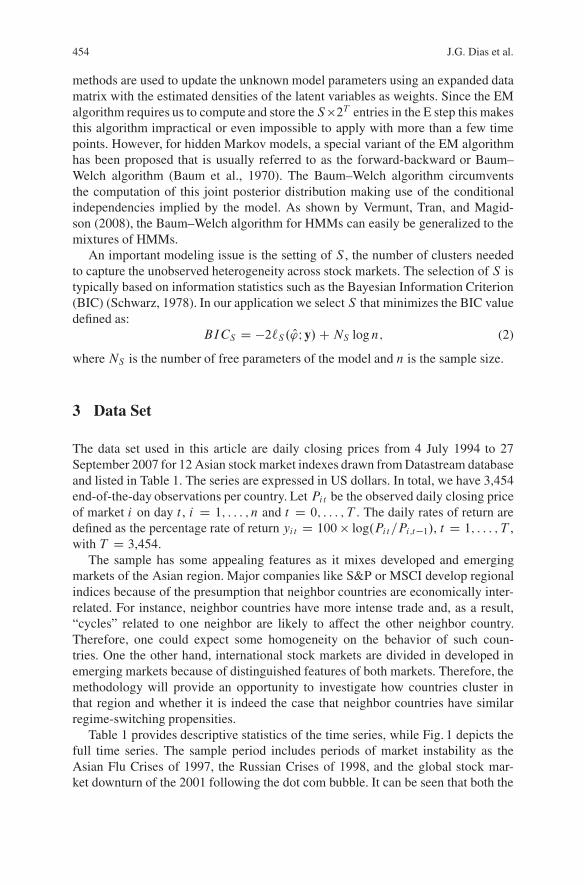
An important modeling issue is the setting of S , the number of clusters neededto capture the unobserved heterogeneity across stock markets. The selection of S istypically based on information statistics such as the Bayesian Information Criterion(BIC) (Schwarz, 1978). In our application we select S that minimizes the BIC valuedefined as:
BICS D �2`S. O'I y/CNS logn; (2)
where NS is the number of free parameters of the model and n is the sample size.
3 Data Set
The data set used in this article are daily closing prices from 4 July 1994 to 27September 2007 for 12 Asian stock market indexes drawn from Datastream databaseand listed in Table 1. The series are expressed in US dollars. In total, we have 3,454end-of-the-day observations per country. Let Pit be the observed daily closing priceof market i on day t , i D 1; : : : ; n and t D 0; : : : ; T . The daily rates of return aredefined as the percentage rate of return yit D 100 � log.Pit =Pi;t�1/, t D 1; : : : ; T ,with T D 3,454.
The sample has some appealing features as it mixes developed and emergingmarkets of the Asian region. Major companies like S&P or MSCI develop regionalindices because of the presumption that neighbor countries are economically inter-related. For instance, neighbor countries have more intense trade and, as a result,“cycles” related to one neighbor are likely to affect the other neighbor country.Therefore, one could expect some homogeneity on the behavior of such coun-tries. One the other hand, international stock markets are divided in developed inemerging markets because of distinguished features of both markets. Therefore, themethodology will provide an opportunity to investigate how countries cluster inthat region and whether it is indeed the case that neighbor countries have similarregime-switching propensities.
Table 1 provides descriptive statistics of the time series, while Fig. 1 depicts thefull time series. The sample period includes periods of market instability as theAsian Flu Crises of 1997, the Russian Crises of 1998, and the global stock mar-ket downturn of the 2001 following the dot com bubble. It can be seen that both the
Mixture Hidden Markov Models 455
Table 1 Summary statistics
Stock market Mean Median Std. deviation Skewness Kurtosis Jarque–Bera testStatistics p-Value
Fig. 1 Time series of index rates for 12 Asian region stock markets
mean and the median return rates are positive and close to zero, except for Japan andThailand. Stock markets show, instead, very diverse patterns of dispersion, wherethe largest standard deviations are found in Thailand, China and Malaysia and thesmallest dispersion in New Zealand and Australia. Higher standard deviations are
456 J.G. Dias et al.
typical for emerging markets, known for their high risk. Return rate distributions arediverse in terms of skewness and the kurtosis (which equals 0 for normal distribu-tions) shows high positive values, indicating heavier tails and more peakness thanthe normal distribution. The Jarque–Bera test rejects the null hypothesis of normal-ity for all 12 stock markets. Overall, these stock market features seem well suited tobe modeled using MHMMs.
4 Results
This section reports the results obtained when applying the MHMM-S describedbefore to these 12 stock markets. We estimated models characterized by differentnumber of clusters (S D 1; : : : ; 8), using for the estimation of each of them 300different starting values for the parameters to avoid local maxima. The model withtwo clusters (S D 2) yielded the lowest BIC value (`2. O'I y/ D �70; 256:1081,N2 D 11 and BIC2 D 140; 539:6).
Table 2 summarizes the results related to the distribution of stock market acrossclusters which gives the size of each cluster. The prior class membership probabilityshows that both clusters have the same size. From the posterior class membershipprobabilities, the probability of belonging to each of the clusters conditional onthe observed data (Table 2), we found six countries assigned to cluster 1 (China,India, Japan, Pakistan, Taiwan, and Thailand) and six countries as well assigned tocluster 2 (Australia, Hong Kong, Malaysia, New Zealand, Philippines, and Singa-pore). Notice that from the posterior probabilities the modal allocation into classesis precise (the probability of the most likely cluster is always one or very closeto one). Notice also that cluster 1 has mostly emerging market countries with theexception of the Japan, while cluster 2 is composed mainly by developed countrieswith the exception of Malaysia and Philippines. By combining the classification
Table 2 Estimated prior and posterior probabilities, and modal clusters for the MHMM-2
information with the descriptive statistics in Table 1, Cluster 1 tends to containcountries with higher volatility (except Japan) and cluster 2 aggregates countrieswith lower volatility, except mainly Malaysia. As it will become clear the maindiscrimination between these two groups has to do with other important factors.
Table 3 provides information on the two regimes that were identified; that is, theaverage proportion of markets in regime k over time and the mean and variance ofthe returns in regime k. The result is in line with the common dichotomization offinancial markets into “bull” and “bear” markets. Consistently, the reported meansshow that one of the regimes is associated with positive returns (bull market) and theother with negative returns (bear market). The probability of being in the bear andbull regimes is 0.25 and 0.75, respectively. We would also like to emphasize thatthese results are coherent with the common acknowledgment of volatility asymme-try of financial markets. Volatility is likely to be higher when markets fall than whenmarkets rise.
Table 4 reports the estimated probabilities of being in one of the regimes withineach cluster. There is a clear distinction between these clusters. Cluster 1 has thelargest probability of being in bear regime (0.35). For cluster 2 this probabilitybecomes 0.16. Moreover, Table 4 provides another key insight from our analysis.It gives the transition probabilities between the two regimes for both clusters. First,notice that both clusters show regime persistence. Once a stock market jumps to aregime, it is likely to remain within the same regime for a while, which is coherentwith stylized facts in financial markets. Second, cluster 2 shows lower propensityto move from a bull regime to a bear regime (0.012) than cluster 1. Third, cluster 1shows higher probability to jump from a bear to a bull regime than cluster 2. This isin line with the idea that cluster 1 has more emerging markets, which are known forhaving more and longer financial crises than developed markets.
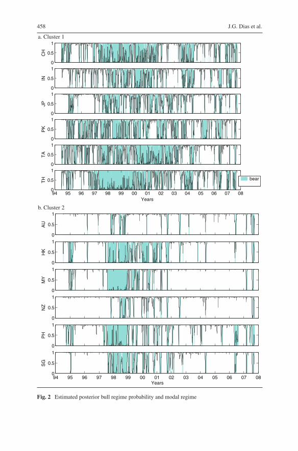
Figure 2 shows the regime-switching dynamics of the countries within both clus-ters. It depicts the posterior probability of being in bull regime at period t , where
458 J.G. Dias et al.
a. Cluster 1
0
0.5
1C
H
0
0.5
1
IN
0
0.5
1
JP
0
0.5
1
PK
0
0.5
1
TA
94 95 96 97 98 99 00 01 02Years
03 04 05 06 07 080
0.5
1
TH bear
b. Cluster 2
0
0.5
1
AU
0
0.5
1
HK
0
0.5
1
MY
0
0.5
1
NZ
0
0.5
1
PH
94 95 96 97 98 99 00 01 02 03 04 05 06 07 080
0.5
1
Years
SG
Fig. 2 Estimated posterior bull regime probability and modal regime
Mixture Hidden Markov Models 459
the grey color identifies periods in which this probability is below 0.5 which corre-sponds to a higher likelihood of being in the bear regime. It is visible a long periodof “bear regimes” that starts at the end of 1997, with the Thailand’s currency crisisand goes until 2002 that affects all the countries of the region. However, the behav-ior before 1997 and after 2002 is clearly different between countries from cluster 1and 2. The two clusters of countries have rather different pattern of regime switch-ing. Cluster 2 is more regime persistent with short duration bear regimes that did notturn out to be endemic during the period of analysis, despite critical periods around1998. Cluster 1 is extremely dynamic and tends to move very fast between regimes,switching frequently between bear and bull states.
5 Conclusions
A mixture of hidden Markov models allows model-based clustering of financial timeseries. In the analysis of a sample of 12 stock markets providing observations for aperiod of 3,454 days the best fitting model was the one with two clusters. The twoclusters clearly defined two distinct types of regime switching, which is coherentwith many stylized facts in finance. Moreover, the simultaneous analysis of the 12time series allows a better comparison of country dynamics in opposition to theapplication of Markov-switching approaches that estimate regimes for each countryseparatively (see, e.g., Wang & Theobald, 2008).
References
Baum, L. E., Petrie, T., Soules, G., & Weiss, N. (1970). A maximization technique occurring inthe statistical analysis of probabilistic functions of Markov chains. Annals of MathematicalStatistics, 41, 164–171.
Dempster, A. P., Laird, N. M., & Rubin, D. B. (1977). Maximum likelihood from incomplete datavia the EM algorithm (with discussion). Journal of the Royal Statistical Society B, 39, 1–38.
Dias, J. G., & Vermunt, J. K. (2007). Latent class modeling of website users’ search patterns:Implications for online market segmentation. Journal of Retailing and Consumer Services, 14,359–368.
Harvey, C. R. (1995). Predictable risk and returns in emerging markets. Review of FinancialStudies, 8, 773–816.
McLachlan, G. J., & Peel, D. (2000). Finite mixture models. New York: Wiley.Schwarz, G. (1978). Estimating the dimension of a model. Annals of Statistics, 6, 461–464.Vermunt, J. K., Tran, B., & Magidson, J. (2008). Latent class models in longitudinal research.
In S. Menard (Ed.), Handbook of longitudinal research: Design, measurement, and analysis(pp. 373–385). Burlington, MA: Elsevier.
Wang, P., & Theobald, M. (2008). Regime-switching volatility of six East Asian emerging markets.Research in International Business and Finance, 22(3), 267–283.