Chapter 20 Mixture Models 20.1 Two Routes to Mixture Models 20.1.1 From Factor Analysis to Mixture Models In factor analysis, the origin myth is that we have a fairly small number, q of real variables which happen to be unobserved (“latent”), and the much larger number p of variables we do observe arise as linear combinations of these factors, plus noise. The mythology is that it’s possible for us (or for Someone) to continuously adjust the latent variables, and the distribution of observables likewise changes continuously. What if the latent variables are not continuous but ordinal, or even categorical? The natural idea would be that each value of the latent variable would give a different distribution of the observables. 20.1.2 From Kernel Density Estimates to Mixture Models We have also previously looked at kernel density estimation, where we approximate the true distribution by sticking a small ( 1 n weight) copy of a kernel pdf at each ob- served data point and adding them up. With enough data, this comes arbitrarily close to any (reasonable) probability density, but it does have some drawbacks. Sta- tistically, it labors under the curse of dimensionality. Computationally, we have to remember all of the data points, which is a lot. We saw similar problems when we looked at fully non-parametric regression, and then saw that both could be amelio- rated by using things like additive models, which impose more constraints than, say, unrestricted kernel smoothing. Can we do something like that with density estima- tion? Additive modeling for densities is not as common as it is for regression — it’s harder to think of times when it would be natural and well-defined 1 — but we can 1 Remember that the integral of a probability density over all space must be 1, while the integral of a re- gression function doesn’t have to be anything in particular. If we had an additive density, f ( x )= j f j ( x j ), ensuring normalization is going to be very tricky; we’d need j f j ( x j )dx 1 dx 2 dx p = 1. It would be easier to ensure normalization while making the log-density additive, but that assumes the features are 390
Transcript
Chapter 20
Mixture Models
20.1 Two Routes to Mixture Models
20.1.1 From Factor Analysis to Mixture ModelsIn factor analysis, the origin myth is that we have a fairly small number, q of realvariables which happen to be unobserved (“latent”), and the much larger number pof variables we do observe arise as linear combinations of these factors, plus noise.The mythology is that it’s possible for us (or for Someone) to continuously adjust thelatent variables, and the distribution of observables likewise changes continuously.What if the latent variables are not continuous but ordinal, or even categorical? Thenatural idea would be that each value of the latent variable would give a differentdistribution of the observables.
20.1.2 From Kernel Density Estimates to Mixture ModelsWe have also previously looked at kernel density estimation, where we approximatethe true distribution by sticking a small ( 1
n weight) copy of a kernel pdf at each ob-served data point and adding them up. With enough data, this comes arbitrarilyclose to any (reasonable) probability density, but it does have some drawbacks. Sta-tistically, it labors under the curse of dimensionality. Computationally, we have toremember all of the data points, which is a lot. We saw similar problems when welooked at fully non-parametric regression, and then saw that both could be amelio-rated by using things like additive models, which impose more constraints than, say,unrestricted kernel smoothing. Can we do something like that with density estima-tion?
Additive modeling for densities is not as common as it is for regression — it’sharder to think of times when it would be natural and well-defined1 — but we can
1Remember that the integral of a probability density over all space must be 1, while the integral of a re-gression function doesn’t have to be anything in particular. If we had an additive density, f (x) =
�j f j (xj ),
ensuring normalization is going to be very tricky; we’d need�
j�
f j (xj )d x1d x2d xp = 1. It would beeasier to ensure normalization while making the log-density additive, but that assumes the features are
390
20.1. TWO ROUTES TO MIXTURE MODELS 391
do things to restrict density estimation. For instance, instead of putting a copy ofthe kernel at every point, we might pick a small number K � n of points, which wefeel are somehow typical or representative of the data, and put a copy of the kernel ateach one (with weight 1
K ). This uses less memory, but it ignores the other data points,and lots of them are probably very similar to those points we’re taking as prototypes.The differences between prototypes and many of their neighbors are just matters ofchance or noise. Rather than remembering all of those noisy details, why not collapsethose data points, and just remember their common distribution? Different regionsof the data space will have different shared distributions, but we can just combinethem.
20.1.3 Mixture ModelsMore formally, we say that a distribution f is a mixture of K component distribu-tions f1, f2, . . . fK if
f (x) =K�
k=1
λk fk (x) (20.1)
with the λk being the mixing weights, λk > 0,�
k λk = 1. Eq. 20.1 is a completestochastic model, so it gives us a recipe for generating new data points: first pick adistribution, with probabilities given by the mixing weights, and then generate oneobservation according to that distribution. Symbolically,
Z ∼ Mult(λ1,λ2, . . .λK ) (20.2)X |Z ∼ fZ (20.3)
where I’ve introduced the discrete random variable Z which says which componentX is drawn from.
I haven’t said what kind of distribution the fks are. In principle, we could makethese completely arbitrary, and we’d still have a perfectly good mixture model. Inpractice, a lot of effort is given over to parametric mixture models, where the fkare all from the same parametric family, but with different parameters — for instancethey might all be Gaussians with different centers and variances, or all Poisson dis-tributions with different means, or all power laws with different exponents. (It’s notstrictly necessary that they all be of the same kind.) We’ll write the parameter, orparameter vector, of the k th component as θk , so the model becomes
f (x) =K�
k=1
λk f (x;θk ) (20.4)
The over-all parameter vector of the mixture model is thus θ= (λ1,λ2, . . .λK ,θ1,θ2, . . .θK ).Let’s consider two extremes. When K = 1, we have a simple parametric distribu-
tion, of the usual sort, and density estimation reduces to estimating the parameters,by maximum likelihood or whatever else we feel like. On the other hand when
independent of each other.
392 CHAPTER 20. MIXTURE MODELS
K = n, the number of observations, we have gone back towards kernel density es-timation. If K is fixed as n grows, we still have a parametric model, and avoid thecurse of dimensionality, but a mixture of (say) ten Gaussians is more flexible than asingle Gaussian — thought it may still be the case that the true distribution just can’tbe written as a ten-Gaussian mixture. So we have our usual bias-variance or accuracy-precision trade-off — using many components in the mixture lets us fit many distri-butions very accurately, with low approximation error or bias, but means we havemore parameters and so we can’t fit any one of them as precisely, and there’s morevariance in our estimates.
20.1.4 GeometryIn Chapter 18, we looked at principal components analysis, which finds linear struc-tures with q space (lines, planes, hyper-planes, . . . ) which are good approximationsto our p-dimensional data, q � p. In Chapter 19, we looked at factor analysis,where which imposes a statistical model for the distribution of the data around thisq -dimensional plane (Gaussian noise), and a statistical model of the distribution ofrepresentative points on the plane (also Gaussian). This set-up is implied by themythology of linear continuous latent variables, but can arise in other ways.
Now, we know from geometry that it takes q+1 points to define a q -dimensionalplane, and that in general any q + 1 points on the plane will do. This means that ifwe use a mixture model with q + 1 components, we will also get data which clustersaround a q -dimensional plane. Furthermore, by adjusting the mean of each compo-nent, and their relative weights, we can make the global mean of the mixture what-ever we like. And we can even match the covariance matrix of any q -factor model byusing a mixture with q + 1 components2. Now, this mixture distribution will hardlyever be exactly the same as the factor model’s distribution — mixtures of Gaussiansaren’t Gaussian, the mixture will usually (but not always) be multimodal while thefactor distribution is always unimodal — but it will have the same geometry, thesame mean and the same covariances, so we will have to look beyond those to tellthem apart. Which, frankly, people hardly ever do.
20.1.5 IdentifiabilityBefore we set about trying to estimate our probability models, we need to make surethat they are identifiable — that if we have distinct representations of the model, theymake distinct observational claims. It is easy to let there be too many parameters, orthe wrong choice of parameters, and lose identifiability. If there are distinct repre-sentations which are observationally equivalent, we either need to change our model,change our representation, or fix on a unique representation by some convention.
• With additive regression, E[Y |X = x] = α+�
j f j (xj ), we can add arbitraryconstants so long as they cancel out. That is, we get the same predictions fromα+ c0+�
j f j (xj )+ c j when c0 =−�
j c j . This is another model of the sameform, α� +�
j f �j (xj ), so it’s not identifiable. We dealt with this by imposing
2See Bartholomew (1987, pp. 36–38). The proof is tedious algebraically.
20.1. TWO ROUTES TO MIXTURE MODELS 393
the convention that α = E[Y ] and E�
f j (Xj )�= 0 — we picked out a favorite,
convenient representation from the infinite collection of equivalent represen-tations.
• Linear regression becomes unidentifiable with collinear features. Collinearityis a good reason to not use linear regression (i.e., we change the model.)
• Factor analysis is unidentifiable because of the rotation problem. Some peoplerespond by trying to fix on a particular representation, others just ignore it.
Two kinds of identification problems are common for mixture models; one istrivial and the other is fundamental. The trivial one is that we can always swap thelabels of any two components with no effect on anything observable at all — if wedecide that component number 1 is now component number 7 and vice versa, thatdoesn’t change the distribution of X at all. This label degeneracy can be annoying,especially for some estimation algorithms, but that’s the worst of it.
A more fundamental lack of identifiability happens when mixing two distribu-tions from a parametric family just gives us a third distribution from the same family.For example, suppose we have a single binary feature, say an indicator for whethersomeone will pay back a credit card. We might think there are two kinds of cus-tomers, with high- and low- risk of not paying, and try to represent this as a mixtureof Bernoulli distribution. If we try this, we’ll see that we’ve gotten a single Bernoullidistribution with an intermediate risk of repayment. A mixture of Bernoulli is al-ways just another Bernoulli. More generally, a mixture of discrete distributions overany finite number of categories is just another distribution over those categories3
20.1.6 Probabilistic Clustering
Yet another way to view mixture models, which I hinted at when I talked about howthey are a way of putting similar data points together into “clusters”, where clustersare represented by, precisely, the component distributions. The idea is that all datapoints of the same type, belonging to the same cluster, are more or less equivalent andall come from the same distribution, and any differences between them are mattersof chance. This view exactly corresponds to mixture models like Eq. 20.1; the hiddenvariable Z I introduced above in just the cluster label.
One of the very nice things about probabilistic clustering is that Eq. 20.1 actuallyclaims something about what the data looks like; it says that it follows a certain dis-tribution. We can check whether it does, and we can check whether new data followsthis distribution. If it does, great; if not, if the predictions systematically fail, then
3That is, a mixture of any two n = 1 multinomials is another n = 1 multinomial. This is not generallytrue when n > 1; for instance, a mixture of a Binom(2,0.75) and a Binom(2,0.25) is not a Binom(2, p)for any p. (EXERCISE: show this.) However, both of those binomials is a distribution on {0,1,2}, andso is their mixture. This apparently trivial point actually leads into very deep topics, since it turns outthat which models can be written as mixtures of others is strongly related to what properties of the data-generating process can actually be learned from data: see Lauritzen (1984). (Thanks to Bob Carpenter forpointing out an error in an earlier draft.)
394 CHAPTER 20. MIXTURE MODELS
the model is wrong. We can compare different probabilistic clusterings by how wellthey predict (say under cross-validation).4
In particular, probabilistic clustering gives us a sensible way of answering thequestion “how many clusters?” The best number of clusters to use is the numberwhich will best generalize to future data. If we don’t want to wait around to get newdata, we can approximate generalization performance by cross-validation, or by anyother adaptive model selection procedure.
20.2 Estimating Parametric Mixture ModelsFrom intro stats., we remember that it’s generally a good idea to estimate distribu-tions using maximum likelihood, when we can. How could we do that here?
Remember that the likelihood is the probability (or probability density) of ob-serving our data, as a function of the parameters. Assuming independent samples,that would be
n�i=1
f (xi ;θ) (20.5)
for observations x1, x2, . . . xn . As always, we’ll use the logarithm to turn multiplica-tion into addition:
�(θ) =n�
i=1log f (xi ;θ) (20.6)
=n�
i=1log
K�k=1
λk f (xi ;θk ) (20.7)
Let’s try taking the derivative of this with respect to one parameter, say θ j .
∂ �
∂ θ j=
n�i=1
1�K
k=1 λk f (xi ;θk )λ j
∂ f (xi ;θ j )
∂ θ j(20.8)
=n�
i=1
λ j f (xi ;θ j )�Kk=1 λk f (xi ;θk )
1f (xi ;θ j )
∂ f (xi ;θ j )
∂ θ j(20.9)
=n�
i=1
λ j f (xi ;θ j )�Kk=1 λk f (xi ;θk )
∂ log f (xi ;θ j )
∂ θ j(20.10)
If we just had an ordinary parametric model, on the other hand, the derivative of thelog-likelihood would be
n�i=1
∂ log f (xi ;θ j )
∂ θ j(20.11)
4Contrast this with k-means or hierarchical clustering, which you may have seen in other classes: theymake no predictions, and so we have no way of telling if they are right or wrong. Consequently, comparingdifferent non-probabilistic clusterings is a lot harder!
20.2. ESTIMATING PARAMETRIC MIXTURE MODELS 395
So maximizing the likelihood for a mixture model is like doing a weighted likelihoodmaximization, where the weight of xi depends on cluster, being
wi j =λ j f (xi ;θ j )�K
k=1 λk f (xi ;θk )(20.12)
The problem is that these weights depend on the parameters we are trying to esti-mate!
Let’s look at these weights wi j a bit more. Remember that λ j is the probabilitythat the hidden class variable Z is j , so the numerator in the weights is the joint prob-ability of getting Z = j and X = xi . The denominator is the marginal probability ofgetting X = xi , so the ratio is the conditional probability of Z = j given X = xi ,
wi j =λ j f (xi ;θ j )�K
k=1 λk f (xi ;θk )= p(Z = j |X = xi ;θ) (20.13)
If we try to estimate the mixture model, then, we’re doing weighted maximum like-lihood, with weights given by the posterior cluster probabilities. These, to repeat,depend on the parameters we are trying to estimate, so there seems to be a viciouscircle.
But, as the saying goes, one man’s vicious circle is another man’s successive ap-proximation procedure. A crude way of doing this5 would start with an initial guessabout the component distributions; find out which component each point is mostlikely to have come from; re-estimate the components using only the points assignedto it, etc., until things converge. This corresponds to taking all the weights wi j to beeither 0 or 1. However, it does not maximize the likelihood, since we’ve seen that todo so we need fractional weights.
What’s called the EM algorithm is simply the obvious refinement of this “hard”assignment strategy.
1. Start with guesses about the mixture components θ1,θ2, . . .θK and the mixingweights λ1, . . .λK .
2. Until nothing changes very much:
(a) Using the current parameter guesses, calculate the weights wi j (E-step)(b) Using the current weights, maximize the weighted likelihood to get new
parameter estimates (M-step)
3. Return the final parameter estimates (including mixing proportions) and clus-ter probabilities
The M in “M-step” and “EM” stands for “maximization”, which is pretty trans-parent. The E stands for “expectation”, because it gives us the conditional probabili-ties of different values of Z , and probabilities are expectations of indicator functions.(In fact in some early applications, Z was binary, so one really was computing theexpectation of Z .) The whole thing is also called the “expectation-maximization”algorithm.
5Related to what’s called “k-means” clustering.
396 CHAPTER 20. MIXTURE MODELS
20.2.1 More about the EM AlgorithmThe EM algorithm turns out to be a general way of maximizing the likelihood whensome variables are unobserved, and hence useful for other things besides mixturemodels. So in this section, where I try to explain why it works, I am going to be abit more general abstract. (Also, it will actually cut down on notation.) I’ll pack thewhole sequence of observations x1, x2, . . . xn into a single variable d (for “data”), andlikewise the whole sequence of z1, z2, . . . zn into h (for “hidden”). What we want todo is maximize
�(θ) = log p(d ;θ) = log�
h
p(d , h;θ) (20.14)
This is generally hard, because even if p(d , h;θ) has a nice parametric form, that islost when we sum up over all possible values of h (as we saw above). The essentialtrick of the EM algorithm is to maximize not the log likelihood, but a lower boundon the log-likelihood, which is more tractable; we’ll see that this lower bound issometimes tight, i.e., coincides with the actual log-likelihood, and in particular doesso at the global optimum.
We can introduce an arbitrary6 distribution on h, call it q(h), and we’ll
�(θ) = log�
h
p(d , h;θ) (20.15)
= log�
h
q(h)q(h)
p(d , h;θ) (20.16)
= log�
h
q(h)p(d , h;θ)
q(h)(20.17)
So far so trivial.Now we need a geometric fact about the logarithm function, which is that its
curve is concave: if we take any two points on the curve and connect them by astraight line, the curve lies above the line (Figure 20.1). Algebraically, this means that
w log t1+ (1−w) log t2 ≤ log w t1+ (1−w)t2 (20.18)
for any 0 ≤ w ≤ 1, and any points t1, t2 > 0. Nor does this just hold for two points:for any r points t1, t2, . . . tr > 0, and any set of non-negative weights
�ri=1 wr = 1,
r�i=1
wi log ti ≤ logr�
i=1wi ti (20.19)
In words: the log of the average is at least the average of the logs. This is calledJensen’s inequality. So
log�
h
q(h)p(d , h;θ)
q(h)≥�
h
q(h) logp(d , h;θ)
q(h)(20.20)
≡ J (q ,θ) (20.21)6Well, almost arbitrary; it shouldn’t give probability zero to value of h which has positive probability
Figure 20.1: The logarithm is a concave function, i.e., the curve connecting any twopoints lies above the straight line doing so. Thus the average of logarithms is less thanthe logarithm of the average.
We are bothering with this because we hope that it will be easier to maximizethis lower bound on the likelihood than the actual likelihood, and the lower boundis reasonably tight. As to tightness, suppose that q(h) = p(h|d ;θ). Then
p(d , h;θ)q(h)
=p(d , h;θ)p(h|d ;θ)
=p(d , h;θ)
p(h, d ;θ)/p(d ;θ)= p(d ;θ) (20.22)
no matter what h is. So with that choice of q , J (q ,θ) = �(θ) and the lower bound istight. Also, since J (q ,θ)≤ �(θ), this choice of q maximizes J for fixed θ.
Here’s how the EM algorithm goes in this formulation.
1. Start with an initial guess θ(0) about the components and mixing weights.
2. Until nothing changes very much
(a) E-step: q (t ) = argmaxq J (q ,θ(t ))
(b) M-step: θ(t+1) = argmaxθ J (q (t ),θ)
3. Return final estimates of θ and q
The E and M steps are now nice and symmetric; both are about maximizing J . It’seasy to see that, after the E step,
J (q (t ),θ(t ))≥ J (q (t−1),θ(t )) (20.23)
398 CHAPTER 20. MIXTURE MODELS
and that, after the M step,
J (q (t ),θ(t+1))≥ J (q (t ),θ(t )) (20.24)
Putting these two inequalities together,
J (q (t+1),θ(t+1)) ≥ J (q (t ),θ(t )) (20.25)
�(θ(t+1)) ≥ �(θ(t )) (20.26)
So each EM iteration can only improve the likelihood, guaranteeing convergence toa local maximum. Since it only guarantees a local maximum, it’s a good idea to try afew different initial values of θ(0) and take the best.
We saw above that the maximization in the E step is just computing the posteriorprobability p(h|d ;θ). What about the maximization in the M step?
�h
q(h) logp(d , h;θ)
q(h)=�
h
q(h) log p(d , h;θ)−�
h
q(h) log q(h) (20.27)
The second sum doesn’t depend on θ at all, so it’s irrelevant for maximizing, givingus back the optimization problem from the last section. This confirms that using thelower bound from Jensen’s inequality hasn’t yielded a different algorithm!
20.2.2 Further Reading on and Applications of EMMy presentation of the EM algorithm draws heavily on Neal and Hinton (1998).
Because it’s so general, the EM algorithm is applied to lots of problems withmissing data or latent variables. Traditional estimation methods for factor analy-sis, for example, can be replaced with EM. (Arguably, some of the older methodswere versions of EM.) A common problem in time-series analysis and signal process-ing is that of “filtering” or “state estimation”: there’s an unknown signal St , whichwe want to know, but all we get to observe is some noisy, corrupted measurement,Xt = h(St ) + ηt . (A historically important example of a “state” to be estimated fromnoisy measurements is “Where is our rocket and which way is it headed?” — seeMcGee and Schmidt, 1985.) This is solved by the EM algorithm, with the signal asthe hidden variable; Fraser (2008) gives a really good introduction to such models andhow they use EM.
Instead of just doing mixtures of densities, one can also do mixtures of predictivemodels, say mixtures of regressions, or mixtures of classifiers. The hidden variableZ here controls which regression function to use. A general form of this is what’sknown as a mixture-of-experts model (Jordan and Jacobs, 1994; Jacobs, 1997) — eachpredictive model is an “expert”, and there can be a quite complicated set of hiddenvariables determining which expert to use when.
The EM algorithm is so useful and general that it has in fact been re-invented mul-tiple times. The name “EM algorithm” comes from the statistics of mixture modelsin the late 1970s; in the time series literature it’s been known since the 1960s as the“Baum-Welch” algorithm.
20.3. NON-PARAMETRIC MIXTURE MODELING 399
20.2.3 Topic Models and Probabilistic LSA
Mixture models over words provide an alternative to latent semantic indexing fordocument analysis. Instead of finding the principal components of the bag-of-wordsvectors, the idea is as follows. There are a certain number of topics which documentsin the corpus can be about; each topic corresponds to a distribution over words. Thedistribution of words in a document is a mixture of the topic distributions. That is,one can generate a bag of words by first picking a topic according to a multinomialdistribution (topic i occurs with probability λi ), and then picking a word from thattopic’s distribution. The distribution of topics varies from document to document,and this is what’s used, rather than projections on to the principal components, tosummarize the document. This idea was, so far as I can tell, introduced by Hofmann(1999), who estimated everything by EM. Latent Dirichlet allocation, due to Bleiand collaborators (Blei et al., 2003) is an important variation which smoothes thetopic distributions; there is a CRAN package called lda. Blei and Lafferty (2009) isa good recent review paper of the area.
20.3 Non-parametric Mixture Modeling
We could replace the M step of EM by some other way of estimating the distributionof each mixture component. This could be a fast-but-crude estimate of parameters(say a method-of-moments estimator if that’s simpler than the MLE), or it could evenbe a non-parametric density estimator of the type we talked about in Chapter 15.(Similarly for mixtures of regressions, etc.) Issues of dimensionality re-surface now,as well as convergence: because we’re not, in general, increasing J at each step, it’sharder to be sure that the algorithm will in fact converge. This is an active area ofresearch.
20.4 Computation and Example: Snoqualmie Falls Re-visited
20.4.1 Mixture Models in R
There are several R packages which implement mixture models. The mclust pack-age (http://www.stat.washington.edu/mclust/) is pretty much standardfor Gaussian mixtures. One of the most recent and powerful is mixtools (Benagliaet al., 2009), which, in addition to classic mixtures of parametric densities, handlesmixtures of regressions and some kinds of non-parametric mixtures. The FlexMixpackage (Leisch, 2004) is (as the name implies) very good at flexibly handling com-plicated situations, though you have to do some programming to take advantage ofthis.
400 CHAPTER 20. MIXTURE MODELS
20.4.2 Fitting a Mixture of Gaussians to Real DataLet’s go back to the Snoqualmie Falls data set, last used in §13.3. There we built asystem to forecast whether there would be precipitation on day t , on the basis ofhow much precipitation there was on day t − 1. Let’s look at the distribution of theamount of precipitation on the wet days.
Figure 20.2 shows a histogram (with a fairly large number of bins), together witha simple kernel density estimate. This suggests that the distribution is rather skewedto the right, which is reinforced by the simple summary statistics
> summary(snoq)Min. 1st Qu. Median Mean 3rd Qu. Max.1.00 6.00 19.00 32.28 44.00 463.00
Notice that the mean is larger than the median, and that the distance from the firstquartile to the median is much smaller (13/100 of an inch of precipitation) than thatfrom the median to the third quartile (25/100 of an inch). One way this could arise,of course, is if there are multiple types of wet days, each with a different characteristicdistribution of precipitation.
We’ll look at this by trying to fit Gaussian mixture models with varying numbersof components. We’ll start by using a mixture of two Gaussians. We could code upthe EM algorithm for fitting this mixture model from scratch, but instead we’ll usethe mixtools package.
The EM algorithm “runs until convergence”, i.e., until things change so little thatwe don’t care any more. For the implementation in mixtools, this means runninguntil the log-likelihood changes by less than epsilon. The default tolerance forconvergence is not 10−2, as here, but 10−8, which can take a very long time indeed.The algorithm also stops if we go over a maximum number of iterations, even if ithas not converged, which by default is 1000; here I have dialed it down to 100 forsafety’s sake. What happens?
> snoq.k2 <- normalmixEM(snoq,k=2,maxit=100,epsilon=0.01)number of iterations= 59> summary(snoq.k2)summary of normalmixEM object:
20.4. COMPUTATION AND EXAMPLE: SNOQUALMIE FALLS REVISITED401
Precipitation in Snoqualmie Falls
Precipitation (1/100 inch)
Density
0 100 200 300 400
0.00
0.01
0.02
0.03
0.04
0.05
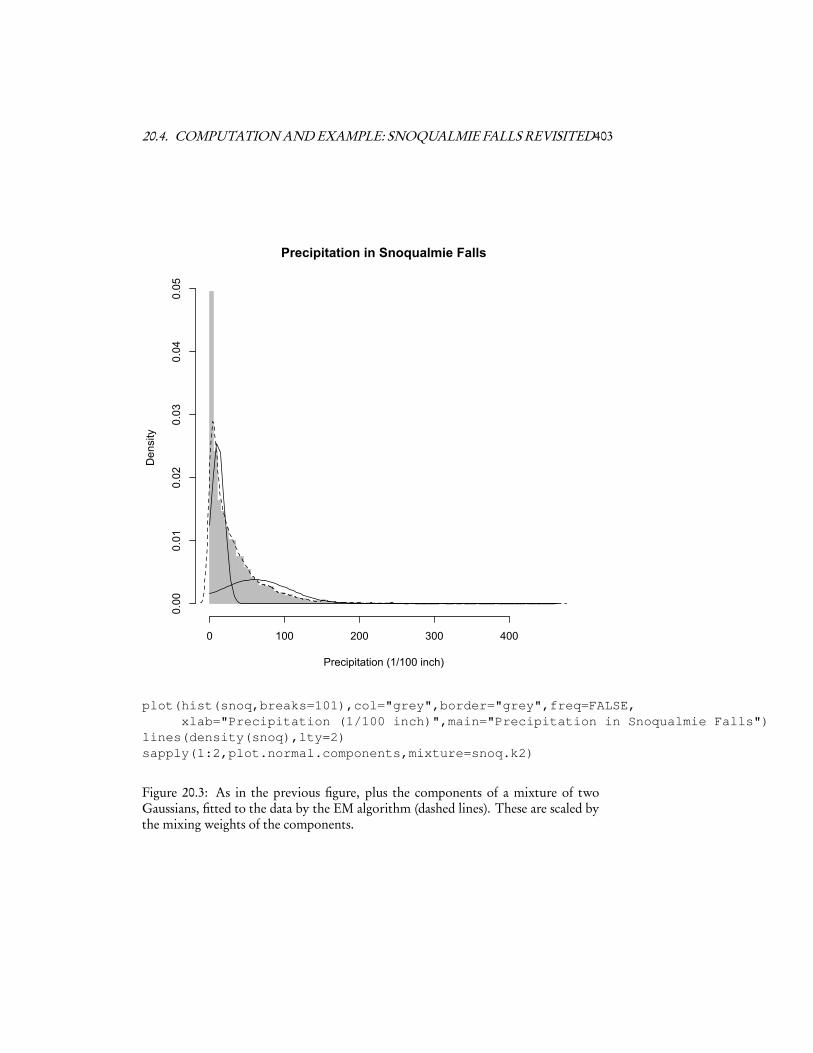
plot(hist(snoq,breaks=101),col="grey",border="grey",freq=FALSE,xlab="Precipitation (1/100 inch)",main="Precipitation in Snoqualmie Falls")
lines(density(snoq),lty=2)
Figure 20.2: Histogram (grey) for precipitation on wet days in Snoqualmie Falls. Thedashed line is a kernel density estimate, which is not completely satisfactory. (It givesnon-trivial probability to negative precipitation, for instance.)
402 CHAPTER 20. MIXTURE MODELS
There are two components, with weights (lambda) of about 0.56 and 0.44, twomeans (mu) and two standard deviations (sigma). The over-all log-likelihood, ob-tained after 59 iterations, is −32681.21. (Demanding convergence to ±10−8 wouldthus have required the log-likelihood to change by less than one part in a trillion,which is quite excessive when we only have 6920 observations.)
We can plot this along with the histogram of the data and the non-parametricdensity estimate. I’ll write a little function for it.
This adds the density of a given component to the current plot, but scaled by theshare it has in the mixture, so that it is visually comparable to the over-all density.
20.4. COMPUTATION AND EXAMPLE: SNOQUALMIE FALLS REVISITED403
Precipitation in Snoqualmie Falls
Precipitation (1/100 inch)
Density
0 100 200 300 400
0.00
0.01
0.02
0.03
0.04
0.05
plot(hist(snoq,breaks=101),col="grey",border="grey",freq=FALSE,xlab="Precipitation (1/100 inch)",main="Precipitation in Snoqualmie Falls")
Figure 20.3: As in the previous figure, plus the components of a mixture of twoGaussians, fitted to the data by the EM algorithm (dashed lines). These are scaled bythe mixing weights of the components.
404 CHAPTER 20. MIXTURE MODELS
20.4.3 Calibration-checking for the MixtureExamining the two-component mixture, it does not look altogether satisfactory — itseems to consistently give too much probability to days with about 1 inch of precip-itation. Let’s think about how we could check things like this.
When we looked at logistic regression, we saw how to check probability forecastsby checking calibration — events predicted to happen with probability p should infact happen with frequency ≈ p. Here we don’t have a binary event, but we dohave lots of probabilities. In particular, we have a cumulative distribution functionF (x), which tells us the probability that the precipitation is ≤ x on any given day.When x is continuous and has a continuous distribution, F (x) should be uniformlydistributed.7 The CDF of a two-component mixture is
F (x) = λ1F1(x)+λ2F2(x) (20.28)
and similarly for more components. A little R experimentation gives a function forcomputing the CDF of a Gaussian mixture:
and so produce a plot like Figure 20.4.3. We do not have the tools to assess whetherthe size of the departure from the main diagonal is significant8, but the fact that theerrors are so very structured is rather suspicious.
7We saw this principle when we looked at generating random variables in Chapter 16.8Though we could: the most straight-forward thing to do would be to simulate from the mixture, and
repeat this with simulation output.
20.4. COMPUTATION AND EXAMPLE: SNOQUALMIE FALLS REVISITED405
Figure 20.4: Calibration plot for the two-component Gaussian mixture. For eachdistinct value of precipitation x, we plot the fraction of days predicted by the mixturemodel to have ≤ x precipitation on the horizontal axis, versus the actual fraction ofdays ≤ x.
406 CHAPTER 20. MIXTURE MODELS
20.4.4 Selecting the Number of Components by Cross-ValidationSince a two-component mixture seems iffy, we could consider using more compo-nents. By going to three, four, etc. components, we improve our in-sample like-lihood, but of course expose ourselves to the danger of over-fitting. Some sort ofmodel selection is called for. We could do cross-validation, or we could do hypothe-sis testing. Let’s try cross-validation first.
We can already do fitting, but we need to calculate the log-likelihood on the held-out data. As usual, let’s write a function; in fact, let’s write two.
dnormalmix <- function(x,mixture,log=FALSE) {lambda <- mixture$lambdak <- length(lambda)# Calculate share of likelihood for all data for one componentlike.component <- function(x,component) {lambda[component]*dnorm(x,mean=mixture$mu[component],
sd=mixture$sigma[component])}# Create array with likelihood shares from all components over all datalikes <- sapply(1:k,like.component,x=x)# Add up contributions from componentsd <- rowSums(likes)if (log) {d <- log(d)
which matches the log-likelihood reported by summary(snoq.k2). But our func-tion can be used on different data!
We could do five-fold or ten-fold CV, but just to illustrate the approach we’ll dosimple data-set splitting, where a randomly-selected half of the data is used to fit themodel, and half to test.
n <- length(snoq)data.points <- 1:ndata.points <- sample(data.points) # Permute randomlytrain <- data.points[1:floor(n/2)] # First random half is training
20.4. COMPUTATION AND EXAMPLE: SNOQUALMIE FALLS REVISITED407
test <- data.points[-(1:floor(n/2))] # 2nd random half is testingcandidate.component.numbers <- 2:10loglikes <- vector(length=1+length(candidate.component.numbers))# k=1 needs special handlingmu<-mean(snoq[train]) # MLE of meansigma <- sd(snoq[train])*sqrt((n-1)/n) # MLE of standard deviationloglikes[1] <- sum(dnorm(snoq[test],mu,sigma,log=TRUE))for (k in candidate.component.numbers) {mixture <- normalmixEM(snoq[train],k=k,maxit=400,epsilon=1e-2)loglikes[k] <- loglike.normalmix(snoq[test],mixture=mixture)
}
When you run this, you will probably see a lot of warning messages saying “Oneof the variances is going to zero; trying new starting values.” The issue is that wecan give any one value of x arbitrarily high likelihood by centering a Gaussian thereand letting its variance shrink towards zero. This is however generally consideredunhelpful — it leads towards the pathologies that keep us from doing pure maximumlikelihood estimation in non-parametric problems (Chapter 15) — so when that hap-pens the code recognizes it and starts over.
If we look at the log-likelihoods, we see that there is a dramatic improvementwith the first few components, and then things slow down a lot9:
(See also Figure 20.5). This favors nine components to the mixture. It looks likeFigure 20.6. The calibration is now nearly perfect, at least on the training data (Figure20.4.4).
9Notice that the numbers here are about half of the log-likelihood we calculated for the two-componentmixture on the complete data. This is as it should be, because log-likelihood is proportional to the numberof observations. (Why?) It’s more like the sum of squared errors than the mean squared error. If we wantsomething which is directly comparable across data sets of different size, we should use the log-likelihoodper observation.
408 CHAPTER 20. MIXTURE MODELS
2 4 6 8 10
-17500
-17000
-16500
-16000
-15500
Number of mixture components
Log-
likel
ihoo
d on
test
ing
data
plot(x=1:10, y=loglikes,xlab="Number of mixture components",ylab="Log-likelihood on testing data")
Figure 20.5: Log-likelihoods of different sizes of mixture models, fit to a random halfof the data for training, and evaluated on the other half of the data for testing.
20.4. COMPUTATION AND EXAMPLE: SNOQUALMIE FALLS REVISITED409
Figure 20.7: Calibration plot for the nine-component Gaussian mixture.
20.4. COMPUTATION AND EXAMPLE: SNOQUALMIE FALLS REVISITED411
20.4.5 Interpreting the Mixture Components, or NotThe components of the mixture are far from arbitrary. It appears from Figure 20.6that as the mean increases, so does the variance. This impression is confirmed fromFigure 20.8. Now it could be that there really are nine types of rainy days in Sno-qualmie Falls which just so happen to have this pattern of distributions, but thisseems a bit suspicious — as though the mixture is trying to use Gaussians systemati-cally to approximate a fundamentally different distribution, rather than get at some-thing which really is composed of nine distinct Gaussians. This judgment relies onour scientific understanding of the weather, which makes us surprised by seeing a pat-tern like this in the parameters. (Calling this “scientific knowledge” is a bit excessive,but you get the idea.) Of course we are sometimes wrong about things like this, soit is certainly not conclusive. Maybe there really are nine types of days, each with aGaussian distribution, and some subtle meteorological reason why their means andvariances should be linked like this. For that matter, maybe our understanding ofmeteorology is wrong.
There are two directions to take this: the purely statistical one, and the substan-tive one.
On the purely statistical side, if all we care about is being able to describe the dis-tribution of the data and to predict future precipitation, then it doesn’t really matterwhether the nine-component Gaussian mixture is true in any ultimate sense. Cross-validation picked nine components not because there really are nine types of days, butbecause a nine-component model had the best trade-off between approximation biasand estimation variance. The selected mixture gives a pretty good account of itself,nearly the same as the kernel density estimate (Figure 20.9). It requires 26 parame-ters10, which may seem like a lot, but the kernel density estimate requires keepingaround all 6920 data points plus a bandwidth. On sheer economy, the mixture thenhas a lot to recommend it.
On the substantive side, there are various things we could do to check the ideathat wet days really do divide into nine types. These are going to be informed by ourbackground knowledge about the weather. One of the things we know, for example,is that weather patterns more or less repeat in an annual cycle, and that different typesof weather are more common in some parts of the year than in others. If, for example,we consistently find type 6 days in August, that suggests that is at least compatiblewith these being real, meteorological patterns, and not just approximation artifacts.
Let’s try to look into this visually. snoq.k9$posterior is a 6920× 9 arraywhich gives the probability for each day to belong to each class. I’ll boil this down toassigning each day to its most probable class:
We can’t just plot this and hope to see any useful patterns, because we want to seestuff recurring every year, and we’ve stripped out the dry days, the division intoyears, the padding to handle leap-days, etc. Fortunately, snoqualmie has all that,so we’ll make a copy of that and edit day.classes into it.
10A mean and a standard deviation for each of nine components (=18 parameters), plus mixing weights(nine of them, but they have to add up to one).
412 CHAPTER 20. MIXTURE MODELS
0 50 100 150 200
020
4060
80
Component mean
Com
pone
nt s
tand
ard
devi
atio
n
1
2345
6
7
8
9
plot(0,xlim=range(snoq.k9$mu),ylim=range(snoq.k9$sigma),type="n",xlab="Component mean", ylab="Component standard deviation")
Figure 20.8: Characteristics of the components of the 9-mode Gaussian mixture. Thehorizontal axis gives the component mean, the vertical axis its standard deviation.The area of the number representing each component is proportional to the compo-nent’s mixing weight.
20.4. COMPUTATION AND EXAMPLE: SNOQUALMIE FALLS REVISITED413
0 100 200 300 400
0.00
0.01
0.02
0.03
0.04
Comparison of density estimates Kernel vs. Gaussian mixture
Precipitation (1/100 inch)
Density
plot(density(snoq),lty=2,ylim=c(0,0.04),main=paste("Comparison of density estimates\n",
"Kernel vs. Gaussian mixture"),xlab="Precipitation (1/100 inch)")
curve(dnormalmix(x,snoq.k9),add=TRUE)
Figure 20.9: Dashed line: kernel density estimate. Solid line: the nine-Gaussian mix-ture. Notice that the mixture, unlike the KDE, gives negligible probability to nega-tive precipitation.
(Note that wet.days is a 36× 366 logical array.) Now, it’s somewhat inconvenientthat the index numbers of the components do not perfectly correspond to the meanamount of precipitation — class 9 really is more similar to class 6 than to class 8. (SeeFigure 20.8.) Let’s try replacing the numerical labels in snoqualmie.classes bythose means.
This leaves alone dry days (still zero) and NA days (still NA). Now we can plot(Figure 20.10).
The result is discouraging if we want to read any deeper meaning into the classes.The class with the heaviest amounts of precipitation is most common in the winter,but so is the classes with the second-heaviest amount of precipitation, the etc. It lookslike the weather changes smoothly, rather than really having discrete classes. In thiscase, the mixture model seems to be merely a predictive device, and not a revelationof hidden structure.11
11A a distribution called a “type II generalized Pareto”, where p(x)∝ (1+ x/σ)−θ−1, provides a decentfit here. (See Shalizi 2007; Arnold 1983 on this distribution and its estimation.) With only two param-eters, rather than 26, its log-likelihood is only 1% higher than that of the nine-component mixture, andit is almost but not quite as calibrated. One origin of the type II Pareto is as a mixture of exponentials(Maguire et al., 1952). If X |Z ∼ Exp(σ/Z), and Z itself has a Gamma distribution, Z ∼ Γ(θ, 1), then theunconditional distribution of X is type II Pareto with scale σ and shape θ. We might therefore investigatefitting a finite mixture of exponentials, rather than of Gaussians, for the Snoqualmie Falls data. We mightof course still end up concluding that there is a continuum of different sorts of days, rather than a finiteset of discrete types.
20.4. COMPUTATION AND EXAMPLE: SNOQUALMIE FALLS REVISITED415
plot(0,xlim=c(1,366),ylim=range(snoq.k9$mu),type="n",xaxt="n",xlab="Day of year",ylab="Expected precipiation (1/100 inch)")
axis(1,at=1+(0:11)*30)for (year in 1:nrow(snoqualmie.classes)) {points(1:366,snoqualmie.classes[year,],pch=16,cex=0.2)
}
Figure 20.10: Plot of days classified according to the nine-component mixture. Hori-zontal axis: day of the year, numbered from 1 to 366 (to handle leap-years). Verticalaxis: expected amount of precipitation on that day, according to the most probableclass for the day.
416 CHAPTER 20. MIXTURE MODELS
20.4.6 Hypothesis Testing for Mixture-Model SelectionAn alternative to using cross-validation to select the number of mixtures is to usehypothesis testing. The k-component Gaussian mixture model is nested within the(k + 1)-component model, so the latter must have a strictly higher likelihood on thetraining data. If the data really comes from a k-component mixture (the null hypoth-esis), then this extra increment of likelihood will follow one distribution, but if thedata come from a larger model (the alternative), the distribution will be different, andstochastically larger.
Based on general likelihood theory, we might expect that the null distribution is,for large sample sizes,
2(log Lk+1− log Lk )∼ χ 2d i m(k+1)−d i m(k) (20.29)
where Lk is the likelihood under the k-component mixture model, and d i m(k) is thenumber of parameters in that model. (See Appendix B.) There are however severalreasons to distrust such an approximation, including the fact that we are approxi-mating the likelihood through the EM algorithm. We can instead just find the nulldistribution by simulating from the smaller model, which is to say we can do a para-metric bootstrap.
While it is not too hard to program this by hand (Exercise 4), the mixtoolspackage contains a function to do this for us, called boot.comp, for “bootstrapcomparison”. Let’s try it out12.
# See footnote regarding this next commandsource("http://www.stat.cmu.edu/~cshalizi/402/lectures/20-mixture-examples/bootcomp.R")snoq.boot <- boot.comp(snoq,max.comp=10,mix.type="normalmix",
maxit=400,epsilon=1e-2)
This tells boot.comp() to consider mixtures of up to 10 components (just aswe did with cross-validation), increasing the size of the mixture it uses when thedifference between k and k + 1 is significant. (The default is “significant at the 5%level”, as assessed by 100 bootstrap replicates, but that’s controllable.) The commandalso tells it what kind of mixture to use, and passes along control settings to the EMalgorithm which does the fitting. Each individual fit is fairly time-consuming, andwe are requiring 100 at each value of k. This took about five minutes to run on mylaptop.
This selected three components (rather than nine), and accompanied this decisionwith a rather nice trio of histograms explaining why (Figure 20.11). Remember thatboot.comp() stops expanding the model when there’s even a 5% chance of thatthe apparent improvement could be due to mere over-fitting. This is actually prettyconservative, and so ends up with rather fewer components than cross-validation.
12As of this writing (5 April 2011), there is a subtle, only-sporadically-appearing bug in the version ofthis function which is part of the released package. The bootcomp.R file on the class website containsa fix, kindly provided by Dr. Derek Young, and should be sourced after loading the package, as in thecode example following. Dr. Young informs me that the fix will be incorporated in the next release of themixtools package, scheduled for later this month.
20.4. COMPUTATION AND EXAMPLE: SNOQUALMIE FALLS REVISITED417
1 versus 2 Components
Bootstrap LikelihoodRatio Statistic
Frequency
0 5 10 15
010
2030
2 versus 3 Components
Bootstrap LikelihoodRatio Statistic
Frequency
0 1000 2000 3000 4000 5000
020
4060
80100
3 versus 4 Components
Bootstrap LikelihoodRatio Statistic
Frequency
0 500 1500 2500
020
4060
80
Figure 20.11: Histograms produced by boot.comp(). The vertical red lines markthe observed difference in log-likelihoods.
418 CHAPTER 20. MIXTURE MODELS
Let’s explore the output of boot.comp(), conveniently stored in the objectsnoq.boot.
> str(snoq.boot)List of 3$ p.values : num [1:3] 0 0.01 0.05$ log.lik :List of 3..$ : num [1:100] 5.889 1.682 9.174 0.934 4.682 .....$ : num [1:100] 2.434 0.813 3.745 6.043 1.208 .....$ : num [1:100] 0.693 1.418 2.372 1.668 4.084 ...
$ obs.log.lik: num [1:3] 5096 2354 920
This tells us that snoq.boot is a list with three elements, called p.values, log.likand obs.log.lik, and tells us a bit about each of them. p.values contains thep-values for testing H1 (one component) against H2 (two components), testing H2against H3, and H3 against H4. Since we set a threshold p-value of 0.05, it stoppedat the last test, accepting H3. (Under these circumstances, if the difference betweenk = 3 and k = 4 was really important to us, it would probably be wise to increase thenumber of bootstrap replicates, to get more accurate p-values.) log.lik is itself alist containing the bootstrapped log-likelihood ratios for the three hypothesis tests;obs.log.lik is the vector of corresponding observed values of the test statistic.
Looking back to Figure 20.5, there is indeed a dramatic improvement in the gen-eralization ability of the model going from one component to two, and from two tothree, and diminishing returns to complexity thereafter. Stopping at k = 3 producespretty reasonable results, though repeating the exercise of Figure 20.10 is no moreencouraging for the reality of the latent classes.
20.5. EXERCISES 419
20.5 ExercisesTo think through, not to hand in.
1. Write a function to simulate from a Gaussian mixture model. Check that itworks by comparing a density estimated on its output to the theoretical den-sity.
2. Work through the E- step and M- step for a mixture of two Poisson distribu-tions.
3. Code up the EM algorithm for a mixture of K Gaussians. Simulate data fromK = 3 Gaussians. How well does your code assign data-points to componentsif you give it the actual Gaussian parameters as your initial guess? If you give itother initial parameters?
4. Write a function to find the distribution of the log-likelihood ratio for testingthe hypothesis that the mixture has k Gaussian components against the alter-native that it has k+1, by simulating from the k-component model. Comparethe output to the boot.comp function in mixtools.
5. Write a function to fit a mixture of exponential distributions using the EMalgorithm. Does it do any better at discovering sensible structure in the Sno-qualmie Falls data?
6. Explain how to use relative distribution plots to check calibration, along thelines of Figure 20.4.3.