M.J. Rodwell and T. Jung Research Department · 567 Understanding the Local and Global Impacts of...

567

Understanding the Local and GlobalImpacts of Model Physics Changes:

An Aerosol Example

M.J. Rodwell and T. Jung

Research Department

Published in Quart. J. Roy. Meteorol. Soc., 134, 1479–1497 (2008)

December 2008

Series: ECMWF Technical Memoranda

A full list of ECMWF Publications can be found on our web site under:http://www.ecmwf.int/publications/

Contact: [email protected]

c©Copyright 2008

European Centre for Medium-Range Weather ForecastsShinfield Park, Reading, RG2 9AX, England

Literary and scientific copyrights belong to ECMWF and are reserved in all countries. This publication is notto be reprinted or translated in whole or in part without the written permission of the Director. Appropriatenon-commercial use will normally be granted under the condition that reference is made to ECMWF.

The information within this publication is given in good faith and considered to be true, but ECMWF acceptsno liability for error, omission and for loss or damage arising from its use.

http://www.ecmwf.int/publications/

Local Physics and Global Impacts: An Aerosol Example

Abstract

This study demonstrates the use a package of diagnostic techniques to understand the local and global re-sponses to a given physics change within a general circulation model. Here, the package is applied to thecase of a change in the aerosol climatology in the forecast model of the European Centre for Medium-rangeWeather Forecasts (ECMWF). The largest difference between old and new climatologies is over the Sa-hara where, in particular, soil-dust aerosol is reduced. Conventional diagnostics show that the change leadto improvements in local medium-range forecast skill and reductions in seasonal-mean errors throughoutthe globe. To study the local physics response, short-range tendencies in weather forecasts are diagnosed.These tendencies are decomposed into the contributions from each physical process within the model. Theresulting ‘initial tendency’ budget reveals how the local atmosphere responds to the aerosol change. Thenet tendencies also provide strong evidence to confirm that the new aerosol climatology is superior. Sea-sonal integrations demonstrate that the tropic-wide response can be understood in terms of equatorial wavesand their enhancement by diabatic processes. The so-called ‘Rossby-wave source’ is made applicable togeneral circulation models and used to understand how the tropical anomalies subsequently impact on theglobal circulation. The mean response in the extratropics is found to be a stationary wave field. Precipita-tion anomalies that are co-located with extratropical divergent vorticity sources suggest the possibility fordiabatic modification of the tropically-forced Rossby-wave response.

1 Introduction

It has long been recognised that localised tropical latent heating anomalies can have an influence on the globalcirculation. The tropical response to such localised heating has been discussed in terms of dynamical equatorialwaves (Matsuno, 1966; Gill, 1980; Heckley and Gill, 1984). Midlatitude responses are often discussed in termsof ‘teleconnection patterns’ (Horel and Wallace, 1981; Hoskins and Karoly, 1981). A knowledge of globalteleconnections is essential for understanding the global climate and is useful for identifying remote ‘causes’of observed seasonal-mean anomalies (Hoskins and Sardeshmukh, 1987).

Teleconnection patterns can be well simulated in models by imposing a prescribed (tropical) convective heatinganomaly (Webster, 1972; Hoskins and Karoly, 1981; Hoskins and Rodwell, 1995; Greatbatch and Jung, 2007)or, more directly still, by imposing the upper-tropospheric divergence anomaly associated with convectiveoutflow (Sardeshmukh and Hoskins, 1988). These studies have been essential to separate the dynamics of tele-connections from the physical mechanisms involved in their initiation. However, if extended-range predictions,such as of monthly or seasonal-mean anomalies, are to benefit from the existence of teleconnectivity, then the(parametrized) physical mechanisms need to be well represented too.

Here two methodologies are brought together to gain a more complete understanding of the local and global im-pacts associated with a model physics change. Firstly the ‘initial tendency’ methodology Rodwell and Palmer(2007), a development of that used by Klinker and Sardeshmukh (1992), is used to understand the local physicswithin a model. The methodology incorporates data assimilation as used in numerical weather forecastingso that model physics can be tested at atmospheric states as close as possible to true atmospheric conditions.A second methodology is developed from the ‘Rossby-wave source’ approach of Sardeshmukh and Hoskins(1988). Assuming that the model change predominantly affects tropical physics, this second methodology isused to identify and understand the extratropical stationary wave response.

The methodologies are applied here to a change in aerosol climatology within the physics of the ECMWFmodel. It is well know that aerosol can have a significant impact on local and global climate (e.g. Miller and Tegen,1998; Menon et al., 2002; Chou et al., 2005; Yoshioka et al., 2007). The aerosol change investigated in thisstudy is predominantly a change in Saharan soil-dust. Plumes of this dust are occasionally seen over the subtrop-ical north Atlantic (Goudie and Middleton, 2001) and these are of global climatological importance because oftheir radically different albedo to that of the underling ocean. At shorter timescales, Saharan aerosol has a very

Technical Memorandum No. 567 1


direct impact on local dust storms associated with the Harmattan. However, Rodwell (2005) and Tompkins et al.(2005) have recently demonstrated that this Saharan aerosol can also have an impact on medium-range weatherforecasts themselves. This paper applies the above methodologies to investigate the impact of the aerosolchange on the local physics and the global dynamics of an atmospheric model in the presence of prescribed (re-alistic) sea-surface temperatures. At seasonal and longer timescales, interactions between the atmosphere andthe ocean begin to modify the response to aerosol (Miller and Tegen, 1998; Miller et al., 2004a; Yoshioka et al.,2007) but these longer timescales and questions such concerning the coupled climate response to aerosol arebeyond the scope of the present study.

Hence this paper can be viewed in two ways. It can be viewed as a demonstration of some key diagnosticmethodologies that could be applied more widely to general circulation models. In this context, the advancemade by the present study is in putting these methodologies together to form a ‘seamless’ package for modelassessment. Alternatively, the paper can be viewed in more specific terms as an estimation of the impact of the(direct) effects of aerosol on local weather and on the global circulation.

In section 2, details are given of the data used and of the salient aspects of the ECMWF model. More specificdetails are then given on the aerosol change that is being studied here. The two types of model simulationsmade are then explained. Finally in this section there is a short note on the use of statistical testing. In section3, the differences seen when the aerosol climatology is modified in the June–August season are documented.The initial tendency methodology is introduced and used to understand the local physics changes in the Saharanregion. Equatorial wave theory and the possibility for interaction with diabatic processes is used to explain thetropic-wide response. The Rossby-wave source diagnostic is made applicable to general circulation models andused to understand the global impacts of the aerosol change. A short sub-section then documents the effects onsurface fluxes of heat and momentum (in the atmospheric model). Section 4, discusses more briefly a parallelstudy of the December–February season. Finally conclusions are given in section 5.

2 Model and Data

2.1 Observational data

Upper-air fields for the period 1962–2001 come from the ECMWF 40-year Re-Analysis dataset (ERA-40,Uppala et al., 2005). This dataset is derived using the 3-dimensional variational data assimilation system. Thedata assimilation process ingests data from almost all available sources. These include top-of-the-atmosphereradiative fluxes at many different wavelengths obtained from satellites as well as radiosonde ascents, drop-sondes and ‘SYNOP’ station reports.

Precipitation observations for the period 1980–1999 come from Xie and Arkin (1997).

Top-of-the-atmosphere radiative fluxes come from the satellite-based ”Clouds and the Earth’s Radiant EnergySystem” (CERES) instrument (Wielicki et al., 1996).

Air-sea fluxes for the period 1980–1993 come from the modified version of the Southampton OceanographyCentre’s climatology (Grist and Josey, 2003). In this version, hydrographic ocean heat transport estimates areused to help constrain the surface fluxes over the Atlantic and North Pacific oceans.

2 Technical Memorandum No. 567


2.2 Model description

A detailed description of the ECMWF model can be found at http://www.ecmwf.int/research/ifsdocs/. In thissection, a brief overview is given of the radiation and convection schemes that were operational in the modelversions used in this study. These are the two physical processes most affected by the aerosol climatologychange. Note that more recent versions of the model, not used here, include updates to both the radiation andconvection schemes.

The radiative heating rate is computed as the vertical divergence of the net radiation flux. Long-wave radiationis computed for 16 spectral intervals using the ‘Rapid Radiation Transfer Model’ (RRTM, Mlawer et al., 1997).The short-wave radiation part, which is computed for 6 spectral intervals, is a modified version of the schemedeveloped by Fouquart and Bonnel (1980). Since the computation of the radiative transfer equation is very ex-pensive, the radiation scheme is ordinarily called at 3-hourly intervals and on a lower-resolution grid. Temporaland spatial interpolation are used to get these calculations onto the model grid. In some of the experiments inthis study (see below) it has been important to call the radiation scheme at every timestep.

Cumulus convection is parametrized by a bulk mass flux scheme which was originally described by Tiedtke(1989). The scheme considers deep, shallow and mid-level convection. Clouds are represented by a single pairof entraining/detraining plumes which describe updraught and downdraught processes.

The ECMWF model uses spherical harmonics to represent the prognostic fields. These harmonics are (trian-gularly) truncated at some total wavenumber, M. With the introduction of a two time-level semi-Lagrangianadvection scheme in 1998, a linear, rather than quadratic, grid has been used for the calculation of physical ten-dencies. The triangular resolution is therefore defined as TLM, and this equates approximately to a resolutionin degrees of 180o/M (the half wavelength of the shortest resolved zonal wave at the equator).

2.3 Aerosol changes

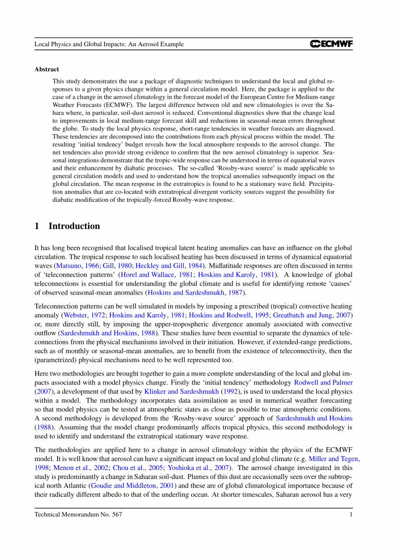
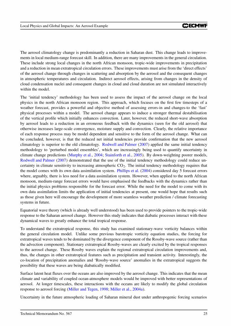
Until October 2003, the aerosol climatology used in the ECMWF operational forecasting model was based onthat of Tanre et al. (1984). This climatology is specified as annual mean geographical distributions of variousaerosol types: ‘maritime’, ‘continental’, ‘urban’, ‘desert’. Each aerosol type has a fixed vertical profile thatdecays exponentially with height. The scale height is set at 3 km for all aerosol types except black carbonwhich has a scale height of 1 km. In addition, uniformly distributed stratospheric background aerosols areincluded. This aerosol climatology (based on Tanre et al., 1984) will be referred to here as the ‘old aerosol’.Figure 1(a) shows the geographical distribution of the total optical depth for the old aerosol at 550 nm (anoptical depth of d for a particular wavelength attenuates radiation at that wavelength by a factor e−d as it passesthrough the atmosphere. This attenuation can be by scattering and absorption). The maximum optical depth(0.74) is seen to occur over the Sahara and this is dominated by desert (i.e.soil dust) aerosol.

In October 2003, a new aerosol climatology was implemented in the ECMWF forecast system (at cycle 26R3).This climatology is based on global maps of optical depths for a range of aerosol types compiled by Tegen et al.(1997). The aerosol types included are sea-salt, soil-dust, sulphate, organic carbon and black carbon. (Back-ground stratospheric aerosol was left unchanged). Atmospheric loading for a given aerosol type is deducedfrom emission/transport modelling studies. For example, soil-dust loading is deduced with eight particle sizeclasses between 0.01 and 10 µm. Uplift from the surface is a function of near-surface windspeed, soil moistureand soil texture. The smallest particles have an atmospheric lifetime of around 230 hours in the transport model,with rain-out being the primary deposition mechanism. The larger particles have a shorter lifetime of around30 hours and deposition is primarily by gravitational settlement. The differing lifetimes lead to a particle sizedistribution in the atmosphere. The optical depth at a given wavelength is a function of atmospheric loading,



60°S

30°S

0°

30°N

60°N

90°W 0° 90°E

(a) Tanre (Annual)

60°S

30°S

0°

30°N

60°N

90°W 0° 90°E

(b) Tegen (Jan)

60°S

30°S

0°

30°N

60°N

90°W 0° 90°E

(c) Tegen (Jul)

Figure 1: Optical depths at 550 nm associated with the model aerosol climatology. (a) The ‘old’ annually-fixed clima-tology of Tanre et al. (1984). (b) The ‘new’ January climatology of Tegen et al. (1997). (c) The ‘new’ July climatology ofTegen et al. (1997). The smallest contour is 0.1 and the contour interval is 0.1.

particle effective radius and refractive index. This climatology (based on Tegen et al., 1997) will be referredto here as the ‘new aerosol’. In this paper, where a difference between two fields, forecasts or simulations isshown, it is in the sense of new aerosol minus old aerosol. This difference will be referred to as the ‘anomaly’or ‘anomalous field’.

For the new aerosol climatology in July (Figure 1(c)) the region of maximum total optical depth (maximising ata value of 1.05) is now located over the Horn of Africa and out into the Arabian Sea associated with the transportof dust by the monsoonal Somali Jet. The aerosol optical depth over the Sahara is more than halved. TheJanuary aerosol of the new climatology (Figure 1(b)) also shows major differences with the old annual-meanclimatology (Figure 1(a)). The magnitude of these changes is comparable with the uncertainties in mineral dustloadings summarised by Zender et al. (2004).

For the short-wave, in addition to being able to scatter radiation, some aerosol types such as soil-dust and blackcarbon can also absorb. By absorbing short-wave radiation, these aerosols can have a very direct impact onatmospheric temperatures. A measure of the relative strength of absorption is given by the ‘single scatteringalbedo’. This is the ratio of scattering efficiency to total light extinction (scattering plus absorption). Thesingle scattering albedo and other aerosol optical properties used within the ECMWF forecasting system are



calculated following Hess et al. (1998). For desert aerosol, the single scattering albedo is around 0.888. Forclean maritime air it is around 0.997. Since the differences between the new and old aerosol are particularlyassociated with desert aerosol, it is possible that absorption as well as scattering will be an important mechanismin the response. For the long-wave, there is no explicit representation of scattering by aerosol in the model.Absorption and emission of long-wave radiation is calculated over all long-wave spectral intervals.

The exponential vertical profiles of particle distribution are left the same in the new aerosol climatology as inthe old climatology.

In the ECMWF model, the aerosol concentration does not impact the cloud microphysics. Hence indirectaerosol effects such as how larger numbers of cloud condensation nuclei can lead to more, smaller and longer-lived cloud droplets and thus changes in the radiation budget are not represented. Instead, the local and globalimpacts of the change in aerosol climatology discussed here must arise purely from the direct effect and the”semi-direct” effect. (The term ”semi-direct” is used to describe the mechanism whereby radiation absorptionleads to warming and less cloud, Hansen et al., 1997).

The last decade has seen further advances in aerosol estimation and, in this respect, the ‘new’ aerosol climatol-ogy cannot be considered as state-of-the-art. However, Tegen et al. (1997) show that comparisons with ground-based sun photometer measurements are reasonable and the ‘new’ aerosol climatology remains in ECMWF’soperational forecast model. In this respect, it is clearly worth understanding the effects of this aerosol climatol-ogy within the global circulation.

2.4 Seasonal integrations

To assess the impact of the change in aerosol climatology on the atmospheric model’s own climate, sets ofseasonal integrations have been made for 40 December–February and June–August seasons for the period 1962to 2001. The initial conditions for these integrations are based on 1 April and 1 October analyses from theERA-40 dataset, respectively (the first two months of each forecast were discarded). Sea-surface temperaturesand sea-ice cover are also taken from ERA-40. These are based on monthly-mean values from the HadISSTdataset (Rayner et al., 2003) up to November 1981 and weekly-mean values from the NOAA/NCEP 2D-Vardataset (Reynolds et al., 2002) thereafter. For each season, a set of integrations is made with old and with newaerosol. The integrations use model cycle 26R3 and are run at TL95 (≈ 1.9o) horizontal resolution with 60levels in the vertical and a timestep of 1 hour. In these seasonal integrations, the radiation scheme is calledevery three hours with computations made on a TL95 linear grid.

It should be emphasised that the seasonal-mean climates and climate anomalies that will be shown are thosefrom an atmospheric model in the presence of prescribed, realistic sea-surface temperatures. This approachallows a good investigation of the salient physics and dynamics of the atmospheric response to aerosol. A goodrepresentation of this atmospheric response is a pre-requisite for good atmosphere-ocean coupled simulations.

2.5 Weather forecasts

It is difficult to isolate the direct effect of a particular model change in seasonal or climate simulations becausethis direct effect will be obscured by interactions and feedbacks with the circulation. The use of weatherforecasts can greatly help in this regard because these are initiated from atmospheric states where the circulationis much closer to a real state of the atmosphere. In this study, 10-day weather forecasts are started every 6 hoursfrom 0 UTC on 26 June 2004 to 18 UTC on 26 July 2004 (31 days × 4 times per day). The day 5 verificationtimes of these experiments exactly comprise July 2004.



The weather forecasts are initialised-with, and verified-against, analyses produced by ECMWF’s 4-dimensionalvariational data assimilation system (4DVAR, Rabier et al., 2000). 4DVAR starts with a ‘first guess’ from aprevious model forecast and essentially involves iteratively nudging the non-linear and tangent-linear versionsof the model to the new observations. Hence the analysis can be quite strongly dependent on the model usedwithin the data assimilation. Since forecast errors and tendencies will be diagnosed at very short lead-times, afair comparison of aerosol climatologies requires that two sets of analyses are produced: one set for the modelincorporating each aerosol climatology. This experimental design allows the same ‘initial tendency’ analysis(see below) to be conducted as in Rodwell and Palmer (2007). These experiments are also used to assess theimpact on conventional measures of medium-range forecast skill.

These weather forecast integrations use model cycle 29R1 and are run at TL159 (≈ 1.1o) horizontal resolutionwith 60 levels in the vertical and a timestep of 1

2 hour. In these forecasts, the radiation scheme is called everytimestep with computations carried-out on a TL63 linear grid.

2.6 Statistical testing

Where a statistical test is mentioned in this paper, this refers to a two-sided Student’s t-test of the differenceof means. In every case shown here both distributions are based on the same set of dates and times andso a more powerful paired t-test is performed. Since autocorrelation could reduce the effective number ofdegrees of freedom in a timeseries, this is taken into account by using an auto-regressive model of order one(von Storch and Zwiers, 2001). A ‘dual colour palette’ has been developed in this study to aid the display ofstatistical significance. This approach is used in some of the figures; with bolder colours indicating significantanomalies and the more pale colours indicating non-significance. Where confidence intervals are shown inplots, they are also based on the Student’s t-distribution function and autocorrelation is taken into account inthe same way. In general, an x% significance level can be thought of as a (100− x)% confidence level.

3 The June–August season

This section first documents the climate and forecast skill differences seen when the aerosol climatology ischanged. Later it is shown how the local physics can be understood by examining initial tendencies in weatherforecasts. The tropical response is discussed in terms of physical coupling with equatorial waves and finallythe vorticity forcing by tropical divergent flow anomalies is used to understand the extratropical response.

3.1 Documenting the differences

3.1.1 Seasonal-mean differences

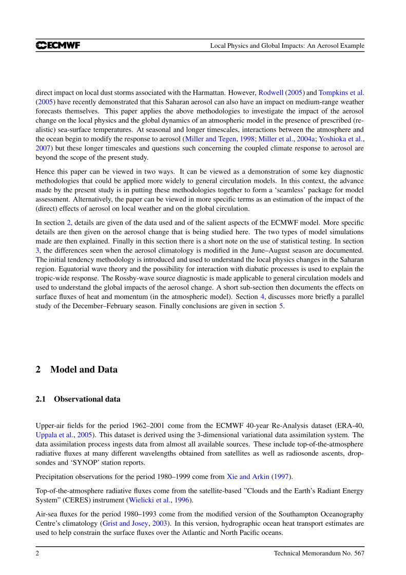
Figure 2(a) shows mean June–August precipitation (shaded), low-level (925 hPa) wind vectors and 500 hPageopotential height contours from the observational data. The summer monsoons of southern Asia, NorthAfrica and Mexico, together with their associated low-level inflows are clearly evident. In the winter (southern)extratropics, a strong westerly jet is evident from the tightness of the geopotential height contours. In thesummer (northern) hemisphere, the jet is weaker.

Figure 2(b) indicates the statistically significant mean errors for the model with the old aerosol. These errorsinclude too much precipitation on the northern flank of the north African monsoon, strong wind biases over thesub-tropical north Atlantic and extratropical circulation biases to the south and southwest of South Africa. The



15 m/s

0° 90°E 180°

(a) JJA OBS

2 4 6 8 10 12 18

5 m/s

0° 90°E 180°

(b) JJA OLD - OBS

-16 -6 -5 -4 -3 -2 -1 1 2 3 4 5 6 16

5 m/s

0° 90°E 180°

(c) JJA NEW - OLD

-10 -5 -2.5 -2 -1.5 -1 -0.5 0.5 1 1.5 2 2.5 5 10

5 m/s

0° 90°E 180°

(d) JJA NEW - OBS

-16 -6 -5 -4 -3 -2 -1 1 2 3 4 5 6 16

Figure 2: Diagnostics of June–August seasonal-mean total precipitation (shaded in mm day−1), 925 hPa horizontal windvectors (see scaling vector) and 500 hPa geopotential heights (see below for contour interval). Observational data comefrom Xie and Arkin (1997) for precipitation over the period 1980–1999 and from ERA-40 for the other fields over theperiod 1962–2001. Forecast data come from the seasonal integrations covering the same period as for the observations(see main text for details). (a) Mean observed. (b) Mean model error with the ‘old’ aerosol. (c) Mean difference: modelwith ‘new’ aerosol minus model with ‘old’ aerosol. (d) Mean model error with the ‘new’ aerosol. Precipitation andwind differences are only plotted where seasonal-mean differences are statistically significant at the 10% level. Heightdifferences are contoured solid for positive, dashed for negative, grey where not significant and with contour interval of10 dam in (a) and 2 dam in (b)–(d).

effect of the change in aerosol (Figure 2(c); note the change in shading interval for precipitation) is a reductionin these particular mean errors so that they are no longer apparent in the mean errors with the new aerosol(Figure 2(d)). Elsewhere, mean errors are largely unchanged. The main degradation is perhaps the increasedmean error in precipitation off the north-east coast of South America.

The north African monsoon will be shown to be a key component in this global improvement. Miller et al.(2004b) show a similar response of north African monsoon precipitation to aerosol forcing, particularly whenparticles are made more absorbing. Yoshioka et al. (2007), who assume weaker absorption, produce a responseof the opposite sign. It would appear that the response can be sensitive to the value of the single scatteringalbedo. At this point in the discussion, it is not possible to say whether the improvement in north Africanmonsoon precipitation occurs for the right or wrong reasons. However, the ‘initial tendency’ discussion laterwill suggest that the improvement is, in fact, for the right reasons.

Assessments of the impact of aerosols often focus on top-of-the-atmosphere ‘forcing’ (e.g. Miller and Tegen,1998). Such forcing is clearly a useful quantity to consider when investigating global climate change. Compar-ison (not shown) between the seasonal integrations and 10 months of CERES data (Wielicki et al., 1996) reveal



that, over the Sahara desert region, there is a reduction in net incoming short-wave radiation error (typicallyfrom +30Wm−2 to +20Wm−2) and also a reduction in out-going long-wave radiation error (typically from−10Wm−2 to near 0Wm−2). Hence, overall, the error in net radiative heating of the atmosphere is reduced(typically from +40Wm−2 to +20Wm−2)). Over the north African monsoon region, incoming short-wave er-rors are also reduced (typically from −15Wm−2 to −5Wm−2). Out-going long-wave radiation errors, however,are increased in the monsoon region (typically from +20Wm−2 to +30Wm−2). Overall the net atmosphericheating error in the monsoon region is unaffected by the aerosol change except along the borders of the Gulf ofGuinea. It should be noted that the simulation of out-going long-wave radiation is more problematic in cloudyregions and so the increase in error in the monsoon region should not, on its own, be interpreted as reflectingunderlying problems with the new aerosol. To emphasise this point further, the typical top-of-the-atmosphere‘forcing’ by the aerosol change is an atmospheric cooling of around 20Wm−2 whereas the atmospheric coolingassociated with the reduction in convective latent heating within the monsoon region (Figure 2(c)) is 4 timeslarger at around 80Wm−2. This suggests the existence of positive feedbacks within the atmospheric responseto aerosol. The apparent error in the out-going long-wave radiation within the monsoon region could easily beassociated with errors in these feedbacks.

While seasonal-mean diagnostics can indicate changes and hopefully improvements in model climate, it isdifficult to obtain a good understanding of how these changes come about. This is particularly the case whenfeedbacks are involved. Later the physics of the local response to the aerosol change will be examined by usingvery short-range forecasts. Next, however, the changes in weather forecast skill will be documented.

3.1.2 Weather prediction differences

It has been shown by Tompkins et al. (2005) that the use of the new aerosol climatology leads to a betterrepresentation of the mean African Easterly Jet in 5-day forecasts with the ECMWF model. Here the focusis on how the use of the new aerosol climatology affects the predictability of variations about the mean inthe North African summer monsoon region. Such variations include fluctuations associated with the AfricanEasterly Jet, including so-called African Easterly waves.

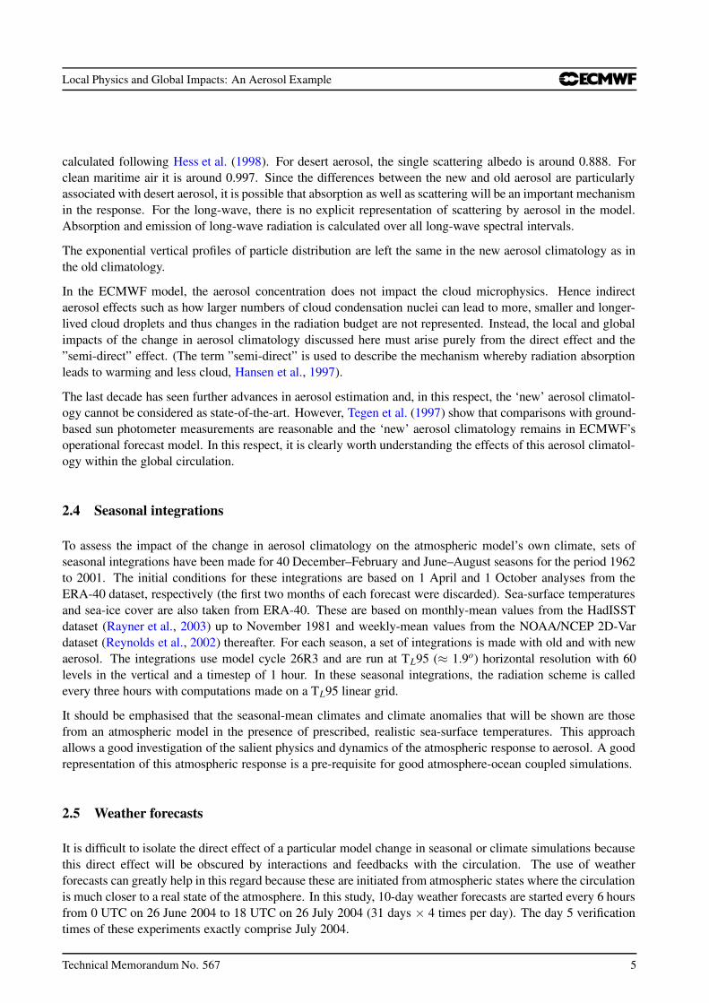
Here, the spatial ‘anomaly correlation coefficient’ is used to quantify the predictive skill of the weather fore-casts. The anomaly correlation coefficient is defined as follows. Let the field ft be the forecast for time t for agiven parameter, region and forecast lead-time. Let the field at be the verifying analysis and let f and a be thetemporal mean fields, averaged over the whole month of forecasts. Remove these mean fields (the part assessedby Tompkins et al. (2005) by writing f′t = ft − f and a′t = at − a. Next remove the area mean (signified by 〈·〉)by writing f′′t = f′t −〈f′t〉 and a′′t = a′t −〈a′t〉. Then the spatial anomaly correlation coefficient is defined here as:

ρt =〈f′′t a′′t 〉

√

〈f′′2t 〉〈a′′2t 〉

. (1)

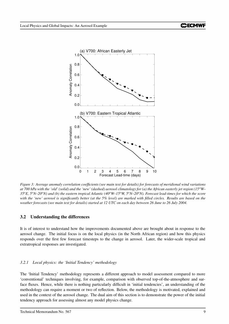
Figure 3(a) shows the seasonal-mean of the spatial anomaly correlation coefficient as a function of forecastlead-time for 700hPa meridional wind field in the African Easterly Jet region [15oW–35oE, 5oN–20oN]. Dotsindicate statistically significant improvements, at the 5% significance level, when the new aerosol is used.Indeed, predictability in the medium-range is increased by about 1 day for each lead-time > 4 days. Similarimprovements are found for the eastern tropical Atlantic region [40oW–15oW, 5oN–20oN] (Figure 3b) and forthe zonal component of the wind in both regions (not shown). Since the aerosol itself is fixed for any givenmonth, these improvements in the prediction of variability must be associated with improvements in simulatingthe mean state. Further-a-field, the skill in forecasting variations about the mean is unaffected by the aerosolchange (not shown).



(a) V700: African Easterly Jet

0.0

0.2

0.4

0.6

0.8

1.0

Ano

mal

y C

orre

latio

n

(b) V700: Eastern Tropical Atlantic

0 1 2 3 4 5 6 7 8 9 10Forecast Lead-time (days)

0.0

0.2

0.4

0.6

0.8

1.0

Ano

mal

y C

orre

latio

n

Figure 3: Average anomaly correlation coefficients (see main text for details) for forecasts of meridional wind variationsat 700 hPa with the ‘old’ (solid) and the ‘new’ (dashed) aerosol climatology for (a) the African easterly jet region (15oW–35oE, 5oN–20oN) and (b) the eastern tropical Atlantic (40oW–15oW, 5oN–20oN). Forecast lead-times for which the scorewith the ‘new’ aerosol is significantly better (at the 5% level) are marked with filled circles. Results are based on theweather forecasts (see main text for details) started at 12 UTC on each day between 26 June to 26 July 2004.

3.2 Understanding the differences

It is of interest to understand how the improvements documented above are brought about in response to theaerosol change. The initial focus is on the local physics (in the North African region) and how this physicsresponds over the first few forecast timesteps to the change in aerosol. Later, the wider-scale tropical andextratropical responses are investigated.

3.2.1 Local physics: the ‘Initial Tendency’ methodology

The ‘Initial Tendency’ methodology represents a different approach to model assessment compared to more‘conventional’ techniques involving, for example, comparison with observed top-of-the-atmosphere and sur-face fluxes. Hence, while there is nothing particularly difficult in ‘initial tendencies’, an understanding of themethodology can require a moment or two of reflection. Below, the methodology is motivated, explained andused in the context of the aerosol change. The dual aim of this section is to demonstrate the power of the initialtendency approach for assessing almost any model physics change.



−4 −2 0 2 4

Mean ∂T/∂t Initial

a

Old

−4 −2 0 2 4

12 96202

353

539

728

884979

Mean ∂T/∂t at day 5

b

Pressure (hP

a)

−4 −2 0 2 4

c

New

−4 −2 0 2 4

12 96202

353

539

728

884979

d

Pressure (hP

a)

−0.8 −0.4 0 0.4 0.8

e

New

−Old

Kday−1

−0.8 −0.4 0 0.4 0.8

12 96202

353

539

728

884979

f

Kday−1

Pressure (hP

a)

Dyn Rad V.Dif Con LSP Net

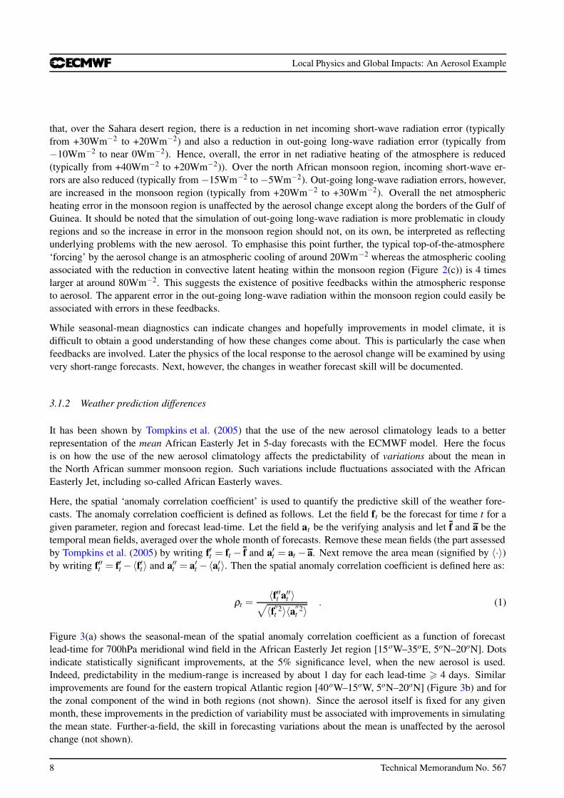
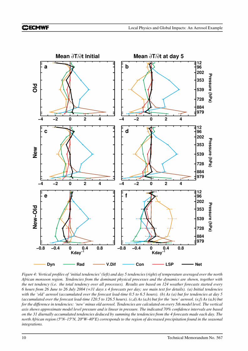
Figure 4: Vertical profiles of ‘initial tendencies’ (left) and day 5 tendencies (right) of temperature averaged over the northAfrican monsoon region. Tendencies from the dominant physical processes and the dynamics are shown, together withthe net tendency (i.e. the total tendency over all processes). Results are based on 124 weather forecasts started every6 hours from 26 June to 26 July 2004 (=31 days x 4 forecasts per day; see main text for details). (a) Initial tendencieswith the ‘old’ aerosol (accumulated over the forecast lead-time 0.5 to 6.5 hours). (b) As (a) but for tendencies at day 5(accumulated over the forecast lead-time 120.5 to 126.5 hours). (c,d) As (a,b) but for the ‘new’ aerosol. (e,f) As (a,b) butfor the difference in tendencies: ‘new’ minus old aerosol. Tendencies are calculated on every 5th model level. The verticalaxis shows approximate model level pressure and is linear in pressure. The indicated 70% confidence intervals are basedon the 31 diurnally accumulated tendencies deduced by summing the tendencies from the 4 forecasts made each day. Thenorth African region (5oN–15oN, 20oW–40oE) corresponds to the region of decreased precipitation found in the seasonalintegrations.



The initial tendency approach involves the use of the weather forecast experiments discussed in section 2.5. Torecapitulate, there are 124 forecasts for each aerosol climatology (31 days × 4 times per day) and the analysisused to initiate a forecast with a particular aerosol is produced by the data assimilation system incorporatingthat same model aerosol.

Each physical and dynamical process within a forecast model contributes to a timestep increment. In this anal-ysis, each process’ contribution is accumulated over the first six hours of the four forecasts made each day.(Actually from lead-time 1

2 hour to lead-time 6 12 hours. This is very different from Klinker and Sardeshmukh

(1992) who examined just the very first forecast timestep. See Rodwell and Palmer (2007) for more discus-sion of these differences). In this way the diurnally-accumulated increment or tendency from each processis produced. These tendencies are then averaged over a chosen region (here the chosen region, 5oN–15oN,20oW–40oE, encompasses the area of reduced June–August north African monsoon rainfall in the seasonalintegrations; Figure 2c). Finally, these diurnally-accumulated, area-averaged tendencies are averaged over the31 days’ of forecasts. The resulting mean tendencies are referred to here as ‘initial tendencies’ as they reflectmean tendencies over the first six hours of a forecast. As will be seen below, initial tendencies are highly usefulbecause they reflect mean tendencies within the model when it is initiated from a set of atmospheric states asclose as possible to the true atmospheric states. (This true atmospheric state includes realistic boundary valuessuch as sea-surface temperatures).

Figure 4(a) shows, for the old aerosol, vertical profiles of the initial tendencies of temperature from the dominantlocal processes. Before discussing these profiles it is worth briefly considering what one might anticipate inthese profiles. The concept of ‘radiative-convective equilibrium’ embodies the idea that radiative processesact to destabilise the atmosphere (heat the surface and cool the mid-to-upper troposphere) and the convectioninduced by this destabilisation acts to restore balance by cooling the surface and heating the mid-to-uppertroposphere. To some extent, Figure 4(a) does show this cancellation between convective (Con) and radiative(Rad) tendencies. However, other terms are also important in the overall balance. In particular, dynamicalcooling associated with ascent (Dyn) and evaporative cooling of large-scale precipitation (LSP) act with theradiation to balance the convective tendency. In the lower troposphere, the vertical diffusion term (V.Dif),which includes the surface sensible heat flux, combines with the radiative tendency (Rad) to destabilise thevertical profile. (Because surface temperatures are strongly dependent on the surface radiation budget, thisdestabilisation by sensible heating can, in fact, be considered as an indirect destabilisation by the radiationprocess). The 70% confidence intervals shown in Figure 4(a) confirm that the 31-day mean tendencies arerobust and not sensitive to the sampling of shorter timescale (e.g. synoptic) variability.

Net initial tendencies (i.e. the sum of initial tendencies from all individual processes) is also displayed inFigure 4(a) (Net). It is important to note that, in the real world, net tendencies should be almost zero whenaccumulated over the diurnal cycle and averaged over sufficient synoptic variability. This is because the nettendency (e.g. of temperature) in the real world is simply the temperature at the end of the period (i.e. month)minus the temperature at the beginning of the period, divided by the length of the period. Typically, for reason-ably large area-means in the tropics and subtropics and for solstitial months, the net temperature tendency is∼0.03 Kday−1. Hence the fact that Figure 4(a) shows non-zero net initial tendencies in the forecast is indicativeof physics errors in the model with the old aerosol (but see below for more discussion). Net initial tendenciesare the seeds of what is termed ‘model drift’ in the climate community. As defined here, these tendencies arevirtually equivalent to minus what is termed the ‘analysis increment’ in the data assimilation community.

To be more precise, to be able to assert that net initial tendencies are indicative of errors in model physics, oneneeds to assume that the climate of the initial state (i.e. the climate of the analysis) is not biased, or at least lessbiased than the climate of the model. This is a reasonable assumption to make since the observations that areused while forming the analysis are a sampling of the real world. As long as the observations are sufficientlyunbiased (they can still be imperfect), so will be the climate of the analysis.



The net initial tendencies in Figure 4(a) (Net) show an erroneous destabilisation of the atmospheric columnin the model with the old aerosol. There is erroneous warming of the lower troposphere (e.g. near 884 hPa)and erroneous cooling of the mid-to-upper troposphere (e.g. near 353 hPa). Referring back to the radiative-convective equilibrium discussion above, one might ask if the radiation scheme is destabilising too much or ifthe convection scheme is not stabilising enough? Of course, at this stage in the investigation the problem couldbe with one or more of the other processes within the atmosphere.

Figure 4(b) shows corresponding tendencies deduced at day 5 of the forecasts (accumulated from lead-time120 1

2 hours to lead-time 126 12 hours). It can be seen that the convective heating (Con) and dynamical cooling

associated with ascent (Dyn) have strongly increased relative to Figure 4(a). In contrast, the net temperaturetendency at day 5 (Net) is smaller than it was in the initial tendencies (Figure 4a). This indicates that, in themean, the forecast model has moved closer to its own preferred equilibrium position by day 5. Consistent withthe seasonal integration results (Figure 2b), this equilibrium occurs at a state with an over-active north Africanmonsoon.

Figure 4(c) shows the initial temperature tendencies for the forecasts with the new aerosol. Interestingly, theinitial convective heating with the new aerosol (Con) is stronger than with the old aerosol (Figure 4a). At firstsight, this is in apparent contradiction to the fact that overall seasonal-mean precipitation is less in the seasonalintegrations with the new aerosol compared to those with the old aerosol (Figure 2c). Importantly, the net initialtendencies in Figure 4(c) (Net) show less erroneous destabilisation of the vertical column with, in particular,less erroneous lower-tropospheric warming than was the case for the old aerosol (Figure 4a).

By day 5 for the new aerosol (Figure 4d), the convective heating and dynamical cooling have again increasedbut the increase is less than with the old aerosol (Figure 4b). This decrease in convection by day 5 relativeto the old aerosol resolves the apparent contradiction highlighted above. Clearly the change in seasonal-meanprecipitation involves not just the changes in initial tendencies but also subsequent feedbacks with the large-scale circulation (as represented by Dyn).

Figure 4(e) shows anomalies (new minus old aerosol) in initial tendencies. Note the change in horizontal axis.The strengthened initial convection (Con) with the new aerosol is clearly evident. However, since indirectaerosol effects are not included in the model, the cloud (included in LSP) and the convection (Con) processescannot be the root-cause of the reduced erroneous net initial tendencies. The root-cause must be associatedwith the interaction between radiation and aerosol.

The anomalous initial radiative tendencies in Figure 4(e) (Rad) show a (direct) cooling over much of the tropo-sphere with increased warming near the surface. The vertical diffusion (V.Dif) also shows increased warmingin the lower-troposphere. (It was mentioned above that the vertical diffusion scheme incorporates the sensibleheat flux and this is itself strongly constrained by the surface radiation budget). The anomalous radiation andvertical diffusion tendencies do not change greatly by day 5 (Figure 4f) whereas the tendencies for the otherdominant processes (Con, Dyn, LSP) do change as they respond to the anomalous aerosol radiative forcing.

There appear, therefore, to be two mechanisms by which the atmosphere responds to the direct radiative effectof the aerosol change:

(1) There appears to be a fast mechanism that is associated with the thermal destabilisation of the verticalprofile. This would appear to lead to the initial enhancement of convection and allow the convection schemeto operate at lower specific humidity levels (the lower-tropospheric moist bias is reduced from 1gkg−1 with theold aerosol to 0.5gkg−1 with the new aerosol, not shown).

(2) There also appears to be a slower mechanism involving interactions with the large-scale dynamics. Theaerosol in this region is primarily soil-dust and it was noted above that soil-dust is able to absorb as well asscatter radiation. The reduction in aerosol therefore leads to the direct cooling of the lower troposphere. This



cooling reduces the erroneous net warming tendency seen with the old aerosol (Figure 4a) and thus acts toreduce the erroneous strengthening of ascent (noted above). With less ascent, there is less large-scale con-vergence and thus the dynamics with the new aerosol provides less moisture to the profile (not shown). Thisslower mechanism appears to provide a limit to the strength of the convection so that by day 5, the convectionis actually less with the new aerosol than it is with the old aerosol.

If these are the two primary response mechanisms then it may be important that the convection deposits itslatent heat above the main aerosol layer. Otherwise the increased initial convection could counter-act the directradiative cooling response to the aerosol change and thus prevent the slow dynamical feedback. Elementsof the semi-direct response to aerosol (whereby radiation absorption by aerosol prevents condensation) couldbe important to ensure that the latent heating is above the main aerosol layer (regardless of which aerosolclimatology is used).

The advantage of the initial tendency approach is that it allows complicated response mechanisms to be diag-nosed before interactions can render the mechanisms impenetrable. Without the initial tendencies one would beforgiven for thinking that the direct effect of the reduced aerosol was reduced monsoon convection. In fact, theinitial effect appears to be increased convection. It is the reduction in the erroneous feedback with the dynamics(Figure 4f, Dyn) that appears to lead to the eventual reduction in erroneous precipitation seen in the seasonal in-tegrations (Figure 2c). Clearly the relative importance of these (and other) mechanisms may be model-specific.In addition, at seasonal and longer timescales, feedbacks with sea-surface temperatures could again modify themonsoon’s response to the aerosol (Miller and Tegen, 1998).

Non-zero net initial tendencies imply errors in model ‘fast physics’ (i.e. physics that has an appreciable effecton numerical weather prediction). In this study the model with the old aerosol has clear physics errors in thelower troposphere over the north African monsoon region (Figure 4a, Net). (The model with either aerosolclimatology appears to have physics errors in the upper troposphere; Figure 4a and c, Net). To make theconverse inference; that smaller net initial tendencies imply smaller errors in model fast physics requires somefurther assumptions to be made.

Firstly, one has to assume that two or more errors cannot cancel each other to leave small net tendencies.Rodwell and Palmer (2007) did assert that cancellation was very unlikely because, over their global domain,the state-space of net initial tendencies has a very high dimension. An upper-bound on this dimension is thetotal number of model grid-points, levels and prognostic variables. Even if the horizontal dimension is reducedto take account of communication by the fastest internal gravity waves over the analysis window (here 6 hours)or simply reduced to the number of distinct climatic regions of the globe (taking into account the phase of theannual cycle), the dimension still remains very large. It would be very unlikely that two distinct model errorscould cancel each other in such a large dimensional space. In the present study, the focus has been on a singleclimatic region and a single prognostic variable and so cancellation may not be quite so unlikely. However,while the discussion above has concentrated on the net initial tendencies of temperature, it is also the case thatthe net initial tendencies of moisture and momentum support the same conclusions.

Secondly, observations are rejected by the data assimilation system if they appear to be ‘too far’ from the firstguess forecast. For an extremely bad model (and thus an extremely bad first guess forecast), many observationscould be rejected. This would leave the analysis close to the first guess and the net initial tendencies would,therefore, be small. However, this is not the case in the present study as the number of tropospheric observationsaccepted by the data assimilation system in the north African monsoon region was actually 2% more for themodel with the new aerosol climatology than for the model with the old aerosol climatology.

In summary, the smaller net initial tendencies over the north African monsoon region with the new aerosolare strong evidence that the new aerosol climatology is superior to the old aerosol climatology. The physicalreasoning based on the initial tendencies is additional evidence. Other evidence has been given including



improvements in seasonal-mean biases and weather forecast skill.

In terms of the present study’s discussion of methodologies for model assessment, it is clear that the initialtendency approach provides a very powerful way of assessing model errors and model changes. Unlike top-of-the-atmosphere fluxes for example, they enable a 3-dimensional examination of the processes involved.They ensure that the observations are used in a consistent manner for both forecast initiation and forecast errorassessment. Importantly, they allow the assessment to be made at atmospheric states close to reality, beforemany interactions and feedbacks have had time to take place. The term ‘close to reality’ refers to the analysis,which is derived from the data assimilation system. Since the analysis can be different for each model underinvestigation, the initial tendency approach also offers something more than can be obtained from single columnmodels forced with fixed boundary conditions. Referring back to the title of this section, initial tendencies allowa very local assessment of model physics. For example, the aerosol changes are predominantly over the northAfrican region but there are differences further-a-field. These differences further-a-field (compare Figure 1aand c) will have impacts on the climate of long model simulations but will have minimal impact on the initialtendencies over north Africa.

3.2.2 Tropical impacts: equatorial waves and diabatic interaction

It has been shown that the direct radiative cooling effect of the aerosol change, and the much stronger nega-tive precipitation response that it triggers, lead to strongly reduced diabatic heating in the June–August seasonwithin the north African monsoon region. Shallow water equation studies on the linearised β -plane (Matsuno,1966; Gill, 1980) demonstrate that such heating anomalies can force equatorial waves. From this theory, onewould anticipate that the weakening of the north African monsoon would force non-dispersive, eastward-propagating Kelvin wave anomalies. In the seasonal-mean, a signature of these waves would be anomalousupwelling over the Indian Ocean. The substantially increased rainfall seen in Figure 2(c) over the northernIndian Ocean / Asian monsoon region (5mmday−1 over the west coast of India) is consistent with a triggeringof convection by these Kelvin waves. If true, this again highlights how the diabatic physics is able to enhancethe dynamical forcing. Note that one can probably discount the possibility that the local increase in aerosol overthe Arabian Sea and Bay of Bengal (compare Figure 1a and c) leads to this increased convection since studiesshow that aerosol increases over the ocean actually lead to a local decrease in precipitation (Miller and Tegen,1998).

Shallow water theory also tells us that the cooling anomaly within the north African monsoon region and theheating anomaly over the northern Indian Ocean will force equatorial Rossby waves. The strengthened cross-equatorial and southwesterly low-level flow over the Arabian Sea in Figure 2(c), for example, is associatedwith the equatorial Rossby-wave response to the Asian monsoon heating anomaly (as in Rodwell and Hoskins,1995). Similarly, the westerly low-level wind anomaly over the tropical Atlantic in Figure 2(c) is consistentwith the reduced north African monsoon heating (Rodwell and Hoskins, 2001).

3.2.3 Extratropical impacts: Rossby-wave forcing

Using the initial tendency analysis, it has been possible to explain the June–August local physical response tothe change in aerosol. The tropic-wide response has been discussed in terms of equatorial wave theory andthe likely enhancement by the diabatic physics. One feature in Figure 2(c) remains to be examined. Thisis the June–August Southern Hemisphere extratropical response which appears as an equivalent barotropicanticyclone–cyclone pair centred to the south of South Africa, with strong southwesterly winds in-between.At 500hPa, this extratropical feature appears disconnected from the tropical changes further north. Two-layershallow water theory, which was used above to interpret tropical, internal, baroclinic waves, is not well suited



to explaining this extratropical, external, equivalent-barotropic response. Instead, it is well known that Rossby-wave dynamics in the upper-troposphere provide the tropical-extratropical link for such a response. Here,Rossby-wave solutions to the vertical vorticity equation are considered. This equation can be written as:

∂ζ∂ t

+∇∇∇ · (vζ ) = 0 , (2)

where ζ is the vertical component of absolute vorticity, t is time and v is the horizontal wind. In equation(2), the shallow atmosphere approximation has been made and vertical advection, tilting, friction and thesolenoidal term have been neglected on scaling arguments for midlatitude synoptic systems. Traditionally(see, e.g. Sardeshmukh and Hoskins, 1988) the wind field is separated into divergent and rotational compo-nents, v = vχ + vψ (where vχ = ∇∇∇χ , the wind component parallel to the gradient of the velocity potential, χ ,and vψ = k×∇∇∇ψ , the wind component parallel to the streamfunction, ψ , and k is the local unit vertical vector)

The components of this equation that are dependent on the divergent flow, vχ , are moved to the right-hand sideof the vorticity equation and regarded as a forcing from the tropics (associated for example with convectiveout-flow changes forced by sea-surface temperature anomalies or, as in this study, with aerosol changes). Theremaining components, which are purely associated with the rotational flow, vψ , are regarded as representingthe extratropical barotropic response:

∂ζ∂ t

+vψ ·∇∇∇ζ = −∇∇∇ · (vχ ζ )

= −ζ∇∇∇ ·vχ −vχ ·∇∇∇ζ .(3)

To emphasis this separation, the right-hand side of equation (3) is sometimes known as the ‘Rossby-wavesource’. The second form of equation (3) splits the Rossby wave source into the divergence component and thecomponent associated with advection by the divergent wind.

Previous studies (e.g. Ting, 1996) have attempted to identify equivalent barotropic levels that best representthe extratropical response to this Rossby wave source. The present study also uses equation (3) to investigatethe vorticity balances in extratropical stationary waves. As in Qin and Robinson (1993), it is found (see later)that the divergence (i.e. ‘stretching’) ‘source’ of vorticity is not negligible in the extratropics and so the rightand left-hand sides of equation (3) are not interpreted so strictly as tropical forcing and extratropical response,respectively.

All the terms in equation (3) except for the local time derivative are quadratic and so they are deduced here ona quadratic Gaussian grid. The calculation is done with the same spectral transforms as used by the ECMWFforecasting system. A scale-selective smoothing is applied that scales a spectral coefficient sm

n , with zonalwavenumber m and total wavenumber n > n0 = 10, by n0(n0 + 1)/(n(n + 1)). If, instead, one sets n0 = 1,then the smoothing would map the Rossby-wave source onto spatial scales compatible with the anomalousstreamfunction, ψ = ∇−2ξ , ψm

n = −ξ mn a2/(n(n+1)), where ξ is relative vorticity, a is the radius of the Earth

and ψ00 = 0. One could argue that these are the scales of interest when examining teleconnections. However,

such a severe smoothing would not allow a good examination of the Rossby-wave dynamics and would, forexample, smooth-away much of the zonal wavenumber 5 wave-guide-mode highlighted by Branstator (2002).With the n0 = 10 smoothing applied here, it is sufficient to truncate the input vorticity and divergence data toT42 as smaller scales have negligible impact after smoothing.

Finally, to ensure that the vorticity analysis is applicable to general circulation models, each term evaluated isvertically integrated between 300 and 100 hPa. The rational for vertically integrating is that relatively minorchanges to model physics can change the level of convective out-flow in the tropics. A Rossby-wave source



Unit: 1e-11 s-2

-7 -5 -3 -1 1 3 5 13 -7 -5 -3 -1 1 3 5 13

1 m/s

Figure 5: June–August mean change in upper tropospheric flow diagnostics from the 40 years of seasonal integrations.Arrows show the change in divergent winds. Shading shows the change in Rossby-wave source derived from daily data.Thick contours show the change in streamfunction. The change is in the sense of ‘new’ minus ‘old’ aerosol. Also shownin thin grey contours is the mean absolute vorticity (the full field is shown; not the change). The diagnostics are derivedfrom the two sets of seasonal integrations (see main text for details). Daily data at 12 UTC is used throughout. Theshading interval for the anomalous Rossby-wave source is generally 2×10−11s−2 but note that orange contours are usedwith the same interval to divide the most extreme (red) colour. The anomalous streamfunction contours are shown at±1, ±3, ±5,... ×106 m2s−1. Contours of the mean absolute vorticity are displayed at ±5, ±10, ±15,... ×10−6s−1. Allquantities are vertically integrated between 300 and 100hPa. Black arrows, black contours and bold shading indicate10% statistical significance for differences of seasonal-means.

diagnostic based on a single level could be strongly affected by this. On the other hand, the strength of the ex-tratropical zonal-mean zonal flow generally maximises at around 200 hPa and is, therefore, reasonably constantover the 300-100 hPa layer. Hence the characteristics of stationary extratropical Rossby-waves are likely to bereasonably similar for all levels between 300 and 100 hPa.

Figure 5 shows the June–August mean of the daily anomalous Rossby-wave source (shaded) from the seasonalintegrations along with the corresponding anomalous divergent wind vectors and anomalous streamfunction(thick contours). Significance, at the 10% level, is indicated by bold shading, black vectors and black contours,respectively. Also shown with thin grey contours is the mean absolute vorticity (averaged over both sets ofseasonal integrations).

The anomalous divergent wind vectors in Figure 5 highlight the anomalous upper-tropospheric convergenceassociated with the weaker north African monsoon and also the increased divergence over southern Asia and thenorthern Indian Ocean (which were associated above with coupling between the convection and the upwellingKelvin-waves). The divergent wind anomaly field associated with these tropical changes has a large-scale andcan be seen to extend into the midlatitudes.

The upper-tropospheric ‘quadrupole’ streamfunction anomaly seen in Figure 5, with low streamfunction anoma-



lies over the subtropical north Atlantic and southern Indian Ocean and high anomalies over the subtropical southAtlantic and Arabian Peninsular (and Capsian Sea), virtually eliminate the mean errors in upper-troposphericstreamfunction in this region relative to the ERA-40 climatology (not shown). Before attempting to understandthis response of the rotational flow to the aerosol change, the Rossby-wave source is first examined.

The mean Rossby-wave source anomaly shown in Figure 5 is calculated from daily data as

−∇∇∇ ·(

vχ ζ)

(N−O)

, (4)

where an overbar indicates a seasonal-mean over 92 days and a second overbar indicates a mean over the 40years of simulations. The supscript (N−O) refers to the new aerosol minus old aerosol.

The strongest Rossby-wave source anomalies are centred over the north coast of Egypt (> 11×10−11s−2) andto the south of South Africa (< −5×10−11s−2). Both these anomalies also act to reduce the mean error in theRossby-wave source relative to ERA-40 (not shown). In both these regions, the anomalous divergent wind isclearly advecting higher magnitude planetary vorticity towards the equator but it will be seen later that this isnot the dominant component of the Rossby-wave source.

The Rossby-wave source is a quadratic term and so it is interesting (from a stationary-wave forcing perspective)to know how important transients are for the time-mean anomaly. Figure 6(a) shows the anomalous Rossby-wave source deduced from seasonal-mean data as

−∇∇∇ ·(

vχ ζ)(N−O)

. (5)

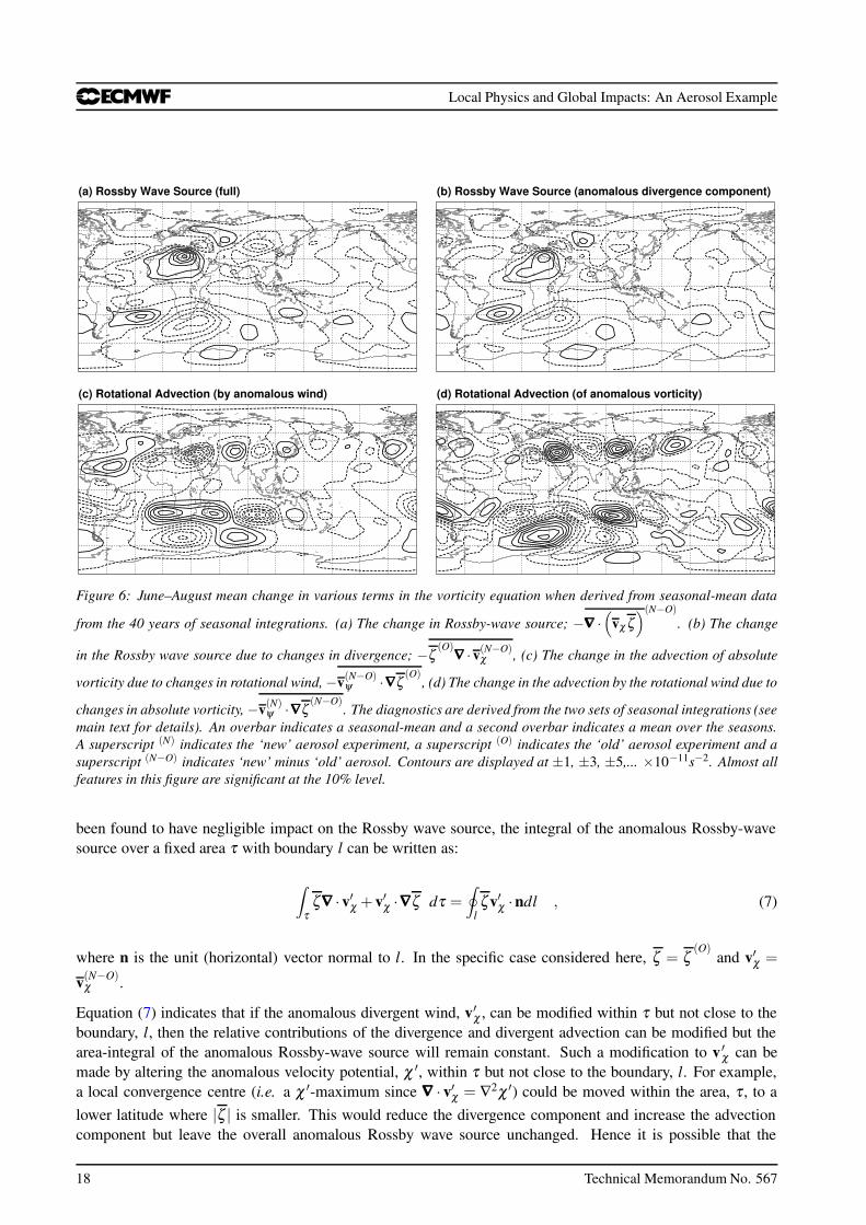
Taking the seasonal mean before calculating the Rossby-wave source should eliminate the effects of transients.The similarity between Figure 6(a) and the anomalous Rossby-wave source shown shaded in Figure 5 demon-strates that the time-mean anomalous Rossby wave-source is essentially unaffected by transient activity.

Equation (5) can be decomposed into four terms:

(

−ζ(O)

∇∇∇ ·v(N−O)χ −v(N−O)

χ ·∇∇∇ζ(O)

−ζ(N−O)

∇∇∇ ·v(N)χ −v(N)

χ ·∇∇∇ζ(N−O)

)

.

(6)

Figure 6(b) shows the first of these four terms (the component associated with anomalous divergence). Thesimilarity with the sum of all four terms (Figure 6a) demonstrates that the source of vorticity associated withanomalous divergence is dominant in the anomalous Rossby-wave source over most of the globe. The third andforth terms in equation (6) (not shown) are found to be negligible. Hence perturbations to the absolute vorticityare not important here for the seasonal-mean anomalous Rossby-wave source. The difference; Figure 6(a)minus (b) is therefore a good approximation for the second term in equation (6); the advection of absolutevorticity by the anomalous divergent wind. It can be seen (by comparing Figure 6a and b) that this term isgenerally also a small component of the Rossby-wave source although it has some contribution over the northcoast of Egypt.

Sardeshmukh and Hoskins (1988) attribute almost the entire anomalous Rossby-wave source in the subtropicalwesterlies to the second term; the advection of absolute vorticity by the divergent flow anomalies. One may askhow this difference of emphasis arises and whether there is an impact on the total Rossby-wave source? Thefollowing integral constraint may partially address this question. As perturbations to the absolute vorticity have



(a) Rossby Wave Source (full) (b) Rossby Wave Source (anomalous divergence component)

(c) Rotational Advection (by anomalous wind) (d) Rotational Advection (of anomalous vorticity)

Figure 6: June–August mean change in various terms in the vorticity equation when derived from seasonal-mean data

from the 40 years of seasonal integrations. (a) The change in Rossby-wave source; −∇∇∇ ·(

vχζ)(N−O)

. (b) The change

in the Rossby wave source due to changes in divergence; −ζ(O)

∇∇∇ ·v(N−O)χ , (c) The change in the advection of absolute

vorticity due to changes in rotational wind, −v(N−O)ψ ·∇∇∇ζ

(O), (d) The change in the advection by the rotational wind due to

changes in absolute vorticity, −v(N)ψ ·∇∇∇ζ

(N−O). The diagnostics are derived from the two sets of seasonal integrations (see

main text for details). An overbar indicates a seasonal-mean and a second overbar indicates a mean over the seasons.A superscript (N) indicates the ‘new’ aerosol experiment, a superscript (O) indicates the ‘old’ aerosol experiment and asuperscript (N−O) indicates ‘new’ minus ‘old’ aerosol. Contours are displayed at ±1, ±3, ±5,... ×10−11s−2. Almost allfeatures in this figure are significant at the 10% level.

been found to have negligible impact on the Rossby wave source, the integral of the anomalous Rossby-wavesource over a fixed area τ with boundary l can be written as:

∫

τζ∇∇∇ ·v′χ +v′χ ·∇∇∇ζ dτ =

∮

lζv′χ ·ndl , (7)

where n is the unit (horizontal) vector normal to l. In the specific case considered here, ζ = ζ(O)

and v′χ =

v(N−O)χ .

Equation (7) indicates that if the anomalous divergent wind, v′χ , can be modified within τ but not close to the

boundary, l, then the relative contributions of the divergence and divergent advection can be modified but thearea-integral of the anomalous Rossby-wave source will remain constant. Such a modification to v ′

χ can bemade by altering the anomalous velocity potential, χ ′, within τ but not close to the boundary, l. For example,a local convergence centre (i.e. a χ ′-maximum since ∇∇∇ · v′χ = ∇2χ ′) could be moved within the area, τ , to alower latitude where |ζ | is smaller. This would reduce the divergence component and increase the advectioncomponent but leave the overall anomalous Rossby wave source unchanged. Hence it is possible that the



stronger emphasis on the divergence term seen here is compensated-for by a reduction in the relative importanceof the advective term, with little impact on the total Rossby-wave source (which is essentially dictated by thetropical convection anomaly). Whether or not this is the full explanation, it is clear that the real world involvescomplexities that are not represented in classical barotropic vorticity equation studies where a non-interactive,idealised, divergence anomaly is used to represent the effects of a (hypothetical) local heating anomaly. Thegeneral conclusion would be that, without prior knowledge of which term is dominant, it is safer to calculatethe total Rossby-wave source.

The response of the rotational flow to this Rossby-wave forcing is now examined. The seasonal-mean of theanomalous local tendency in (the anomaly version of) equation (3) should be negligible and so, where theassumptions made in equation (3) are valid, there should be a balance between the mean anomalous Rossby-wave source and the mean anomalous advection of absolute vorticity by the rotational flow. An interesting firstquestion concerns whether such a time-mean balance can be achieved by a stationary rotational flow anomaly orwhether transients are important for the mean anomalous ‘rotational advection’. It has already been establishedthat transients are not important for the mean anomalous Rossby-wave source. Using the same approach ofcalculating the quadratic term using seasonal-mean rather than daily values, it is found that transients alsohave a negligible impact on the mean rotational advection. This indicates that the rotational flow anomaly,displayed by the streamfunction contours in Figure 5, represents a stationary response to the mean anomalousRossby-wave source.

To first-order, the vorticity balance can therefore be expressed as:

−v(N−O)ψ ·∇∇∇ζ

(O)−v(N)

ψ ·∇∇∇ζ(N−O)

−ζ(O)

∇∇∇ ·v(N−O)χ ≈ 0 .

(8)

This balance is evident in Figure 6 where the first and second terms in equation (8) are displayed in Figure 6(c)and (d), respectively and the third term (the dominant component of the Rossby-wave source), which hasalready been discussed, is shown in Figure 6(b). In addition, in regions where the Rossby-wave source isrelatively small, the first two terms in equation (8) should cancel each other. Physically, this cancellation canbe thought of as the Rossby wave propagating upstream (first term in equation (8), Figure 6c) at the samespeed as it is being advected downstream (second term in equation (8), Figure 6d). This balance is seen ratherbeautifully over Asia and into the North Pacific and reflects a Rossby wave being forced, primarily, by theRossby-wave source (third term in equation (8), Figure 6b) centred over the north coast of Egypt. Meridionaloscillations in the northern-most streamfunction contour over Asia and the north Pacific in Figure 5 reflectthis stationary Rossby wave. This wave is in excellent agreement with the Asian ‘waveguide’ mode producedby Ambrizzi et al. (1995) using a barotropic vorticity equation model (their Fig 16). A balance between thefirst two terms in equation (8) is also seen over the subtropical north Atlantic (compare Figure 6c and d). Theresponse in this region was discussed in section 3.2.2 in terms of classical equatorial Rossby wave theory.However, the present balance emphasises a conclusion of Rodwell and Hoskins (1996) that the westerly flowover the subtropical north Atlantic, and not simply the dissipation term used by Gill (1980), is important for thestationarity of this Rossby wave feature.

In the Southern Hemisphere, Figure 5 indicates that the Rossby-wave source to the southeast of South Africainitiates two Rossby waves, one centred at around 25oS and another centred at around 50oS. Again, this ishighly consistent with Ambrizzi et al. (1995) who discuss a subtropical waveguide and a polar waveguide intheir observational, theoretical and modelling results. It is clear that such waveguide theories are of greatpractical use for the investigation of remote responses to model physics changes. In this study, these two waves



20 m/s

(a) JJA OBS25 75 125 175 225

4 m/s

(b) JJA OLD-OBS-70 -50 -30 -10 10 30 50 70

4 m/s

(c) JJA NEW-OLD-70 -50 -30 -10 10 30 50 70

4 m/s

(d) JJA NEW-OBS-70 -50 -30 -10 10 30 50 70

Figure 7: Diagnostics of June–August seasonal-mean surface latent heat flux (Wm−2), shaded, and 10m wind vectors(ms−1, see reference arrow). Observational data come from Grist and Josey (2003) for surface latent heat flux over theperiod 1980–1993 and from ERA-40 for near-surface wind over the period 1962–2001. Forecast data come from theseasonal integrations covering the period 1962–2001 (see main text for details). (a) Mean observed. (b) Mean modelerror with ‘old’ aerosol. (c) Mean difference: model with ‘new’ aerosol minus model with ‘old’ aerosol. (d) Mean modelerror with ‘new’ aerosol.

have opposite phases, with a high anomaly north of a low anomaly etc. At 50oS, the Rossby wave source(Figure 6b) can be seen to ‘aid’ the advection of mean vorticity by the anomalous rotational winds (Figure 6c).For the wave around 25oS, the Rossby-wave source (Figure 6b) tends to ‘aid’ the advection of anomalousvorticity by the mean rotational winds (Figure 6d). This is a partial explanation for the opposing phases of thetwo waves. Just how the three terms in equation (8) combine to produce a steady flow response may be sensitiveto the mean gradient of absolute vorticity, which is stronger at 25oS than at 50oS. The wave at around 50oS is,as might be expected, more barotropic in nature and this is the wave that dominates the mean mid-troposphericand lower-tropospheric response seen in Figure 2(c).

It is not obvious from these seasonal integrations how the anomalous flow would be set-up over time. Similarplots to Figure 5 have been produced (not shown) based on the 124 weather forecasts (31 days × 4 times perday). These show the evolution of the mean anomaly from the start of the forecast (when the small differencesreflect analysis differences) to a leadtime of 10 days (when the differences are in good agreement with Fig-ure 5). It is found that the divergent and rotational flow anomalies evolve together (rather than the Rossby-wavesource being established first and the rotational flow responding sometime later). The time evolution of the ro-tational flow is consistent with the instantaneous imbalance between the Rossby-wave source and the rotationaladvection. These results imply that aerosol anomalies of the magnitude discussed here can have an impact onextratropical forecasts at lead-times of around 10 days.

Note that equation (8) is not appropriate to describe the vorticity balance over tropical Africa itself. One cansee, for example, that the divergence term (Figure 6b) is not negligible around 15oN,0oE but neither componentof the rotational advection (Figure 6c and d) is able to balance it. Clearly other terms that were neglected in thevorticity equation (2) are important in this small region.



3.2.4 Impact on the coupled ocean-atmosphere system

The aerosol change has been shown to lead to improvements in local atmospheric physics and global atmo-spheric teleconnections. Here, the consequences for coupled ocean-atmosphere models are briefly investigatedby examining surface flux responses in the atmospheric model. There is already evidence that coupled mod-els do respond differently to aerosol radiative forcing, particularly over the oceans (Miller and Tegen, 1998).However, it is difficult when analysing long integrations of coupled models to disentangle the impact on surfacefluxes of (1) the purely-atmospheric response to the aerosol change from (2) the subsequent ocean-atmospherefeedbacks. Here, the purely-atmospheric response is diagnosed by calculating surface fluxes in the seasonalintegrations of the atmospheric model forced with realistic sea-surface temperature. The hope would be thatthe purely-atmospheric response to the change in aerosol leads to an improvement in surface fluxes. Such animprovement would then suggest that the climate of the coupled model would not drift so quickly (or so far)from that of the real world. Before quantifying the atmospheric model’s response, the observed surface (latent)heat fluxes are discussed.

Climatological near-surface wind vectors from ERA-40 and observed turbulent surface latent heat fluxes fromGrist and Josey (2003) are shown in Figure 7(a) for the June–August season. In the tropical and sub-tropicalAtlantic as well as in the Indian ocean, large latent heat fluxes out of the ocean generally coincide with strongnear-surface climatological mean winds. An exception is in the oceanic upwelling regions, such as the easterntropical Atlantic, where relatively small latent heat fluxes coincide with cold sea-surface temperatures.

Mean errors in simulating near-surface wind speed and surface latent heat fluxes are shown in Figure 7(b) forthe model with the old aerosol climatology. By comparing with Figure 7(a) it can be seen that, where meanwind errors enhance the observed climatological winds, the mean latent heat flux errors are positive. Similarly,where mean wind errors oppose the observed climatological winds, the mean latent heat flux errors are negative.

Figures 7(c) and (d) show that the change in aerosol climatology leads to substantial improvements in near-surface wind speeds and, therefore, also the surface latent heat fluxes. This is particularly true for the tropicaland subtropical North Atlantic and the Arabian Sea, where latent heat-flux anomalies amount to as much as±30 Wm−2 (even though sea-surface temperatures are the same for both sets of integrations).

The reduction of mean errors of the ECMWF atmospheric model in simulating turbulent surface heat fluxesmay lead to a reduction of the climate drift (Moore and Gordon, 1994) of ECMWF’s coupled ocean-atmospheremodel, which is used to produce seasonal forecasts. The reduction of mean errors in near-surface winds mayalso lead to important improvements in surface momentum fluxes. Tropical Atlantic surface momentum fluximprovements may, for example, lead to improvements in the tropical Atlantic thermocline tilt and thus im-provements in low-frequency coupled variability.

4 The December – February season

For completeness, some of the sections above are briefly repeated for the December–February season. As wouldbe expected, much of the reasoning given for the June–August season carries over to the December–Februaryseason.

4.1 Seasonal-mean differences

Figure 8 shows a similar plot to Figure 2 but for the December–February season based on the seasonal integra-tions started on 1 October for the years 1962–2001. Figure 8(a) shows mean December–February precipitation,



low-level (925 hPa) winds and 500 hPa geopotential heights from the observational data. The Southern Hemi-sphere summer monsoons over South America, Southern Africa and northern Australia together with their as-sociated low-level inflows are clearly evident. In the winter (northern) extratropics, the westerly jet is strongerthan it was in the June–August season (Figure 2a) while in the summer (southern) hemisphere, the jet is weakerthan it was in the June–August season.

Some of the statistically significant mean errors for the old aerosol integrations (Figure 8b) are reduced whenthe new aerosol is introduced (Figure 8c). These improvements include a reduction in the erroneous precipi-tation over the Gulf of Guinea, a beneficial increase in mean precipitation over the equatorial Indian Ocean, asubstantial reduction in the extratropical high geopotential height bias over the North Pacific and a reductionin the low geopotential height bias centred over the coast of California. These height biases had been long-standing problems for the ECMWF model (e.g. Jung, 2005). The height changes are reflected in the substantialimprovements in mean low-level wind over the North Pacific and (not shown) improvements to synoptic ac-tivity in the North Pacific stormtrack region. Interestingly, Miller and Tegen (1998) also found a statisticallysignificant mean response over the North Pacific to the radiative forcing by dust aerosol. In this study, it willbe demonstrated that these extratropical anomalies are ‘connected’ to those in the tropics through the action ofupper-tropospheric Rossby waves.

4.2 Local physics

The same physical reasoning as given for the June–August season is used to explain how the local physics inDecember–February responds to the change in aerosol. Hence the strong reduction in precipitation over theGulf of Guinea in response to the reduced aerosol (compare Figure 1a,b) is likely to be triggered by reducedshort-wave absorption. However, the strength of the change may be particularly strong over the Gulf of Guineabecause the reduced short-wave absorption is not balanced, over a region of prescribed sea-surface temperature,by surface long-wave, sensible or latent heat fluxes. This explains the great improvement in precipitation in thisregion in terms of the atmospheric model being used here but it also highlights a potential difference betweenatmosphere and coupled ocean-atmosphere simulations. In atmospheric simulations, the ocean effectively hasan infinite heat capacity whereas increased downward short-wave could be expected to increase sea-surfacetemperature in a coupled model and eventually lead to surface fluxes that compensate for the direct atmosphericcooling effect. One may speculate that, in the real world, short timescale fluctuations of aerosol are potentiallymuch more powerful over the ocean than over the land but that this disparity diminishes at longer timescales.

The strong reduction in aerosol over the Sahara (compare Figure 1a and b) also leads to a radiative coolinganomaly (not shown). Although there is no precipitation in this region for this forcing to positively feed-backwith at this time of year, the radiative cooling alone is apparently enough to force some descent and upper-levelconvergence.

4.3 Tropical impacts

With similar reasoning to that for the June–August season, the December–February decrease in precipitationover the Gulf of Guinea and equatorial Africa is likely to force eastward-propagating, upwelling Kelvin wavesover the Indian Ocean. The increased precipitation seen over the tropical Indian Ocean in Figure 8(c) is con-sistent with a diabatic coupling with these waves. Such coupling was speculated for the June–August seasonabove. However, for the December–February season, it is also possible that the reduction in aerosol overthe tropical Indian Ocean itself (compare Figure 1 a and b) could contribute to the increase in precipitation(Miller and Tegen, 1998).



15 m/s

0° 90°E 180°

(a) DJF OBS

2 4 6 8 10 12 18

5 m/s

0° 90°E 180°

(b) DJF OLD - OBS

-16 -6 -5 -4 -3 -2 -1 1 2 3 4 5 6 16

5 m/s

0° 90°E 180°

(c) DJF NEW - OLD

-10 -5 -2.5 -2 -1.5 -1 -0.5 0.5 1 1.5 2 2.5 5 10

5 m/s

0° 90°E 180°

(d) DJF NEW - OBS

-16 -6 -5 -4 -3 -2 -1 1 2 3 4 5 6 16

Figure 8: As Figure 2 but for December–February seasonal-means.

4.4 Extratropical impacts and feedbacks

Figure 9 shows the same upper-tropospheric diagnostics as in Figure 5, but for the December–February season.The tropical divergent wind anomalies, with anomalous convergence towards the Gulf of Guinea and divergencefrom the equatorial Indian Ocean are consistent with the latent heating changes associated with the anomalousprecipitation. The Rossby-wave source centres located over Spain/Morocco and over Afghanistan appear tobe related to the tropical response. Interestingly, these centres are on the northern flank of the subtropicaljet and their signs are opposite to what one would expect from the vorticity advection by the divergent windanomalies south of the subtropical jet. Again, the local divergence term must be dominating the Rossby-wavesource in these regions but a full understanding has not been investigated here. Given that the Rossby-wavesource is as it is in Figure 9, one can see that it is consistent with the wave-train in anomalous streamfunction(thick contours) that spreads along the jetstream to the east. Using the same methodology as used for the June–August season, it is again established that this wave is part of a stationary wave solution. The wave clearlyconnects to the North Pacific anomalies seen in 500hPa geopotential heights (Figure 8c). This stationary wave-train has strong similarities with the circumglobal wave of Branstator (2002). The wave’s path and zonalwavenumber are highly reminiscent of the Asian jet-stream waveguide highlighted by Hoskins and Ambrizzi(1993). Indeed their barotropic vorticity equation model even predicts a southward turning of the stationarywave as it approaches the west coast of North America just as can be seen in Figure 9.

Interestingly, the amplitude of the wave-train in anomalous streamfunction in Figure 9 is relatively large overthe North Pacific. The non-divergent barotropic vorticity equation model of Hoskins and Ambrizzi (1993) alsoshows that the largest amplitude (in relative vorticity anomaly) for their wave in the Asian waveguide is centredover the west Pacific (at around 140oE, 30oN). Although the location is not quite the same as found here,



Unit: 1e-11 s-2

-7 -5 -3 -1 1 3 5 7 -7 -5 -3 -1 1 3 5 7

1 m/s

Figure 9: As Figure 5 but for December–February mean change.

it is clear that non-divergent dynamical processes alone can account for some downstream increase in waveamplitude. In the present study, however, Figure 9 shows that there is also a strong negative ‘Rossby-wavesource’ anomaly centred at 210oE, 40oN. The inverted commas are used around ‘Rossby-wave source’ herebecause the location is far from the tropics and so this vorticity source cannot be viewed as an independentforcing. Instead, this ‘Rossby-wave source’ indicates that divergent processes also play a role in defining thestationary wave pattern over the North Pacific. The main component to this ‘Rossby-wave source’ anomalyis, as before, the divergence term rather than the advection by the divergent wind. One possible origin forthe negative Rossby-wave source term here is adiabatic vortex-tube shrinkage in the anomalous northwardflow. (The anomalous flow is northward because the rotational wind dominates the divergent component shownin Figure 9. Anomalous vortex shrinkage would occur because the isentropic surfaces get closer togethertowards the pole). However, it is intriguing to note that Figure 8(c) shows increased precipitation in thisregion. Increased precipitation would be consistent with upper-tropospheric potential vorticity destruction.Other regions in the north Pacific with reduced precipitation (one such centre is visible in Figure 8(c) at around180oE, 15oN) coincide with the two positive Rossby-wave source anomalies. Hence it is possible, if a littlespeculative at present, that there is some local diabatic modification, or even enhancement, of the tropically-forced stationary Rossby wave taking place over the North Pacific.

5 Conclusions

This paper can be viewed as a sensitivity study and explanation of the effects, local and global, of a change inmodel aerosol climatology. Alternatively, the paper can be seen as the development and seamless applicationof previous methodologies for understanding the general circulation, that could form a diagnostic package toassess almost any physics change within a general circulation model.



The aerosol climatology change is predominantly a reduction in Saharan dust. This change leads to improve-ments in local medium-range forecast skill. In addition, there are many improvements in the general circulation.These include strong local changes in the north African monsoon, tropic-wide improvements in precipitationand a reduction in mean extratropical circulation errors. These improvements must arise from the ‘direct effects’of the aerosol change through changes in scattering and absorption by the aerosol and the consequent changesin atmospheric temperatures and circulation. Indirect aerosol effects, arising from changes in the density ofcloud condensation nuclei and consequent changes in cloud and cloud duration are not simulated interactivelywithin the model.

The ‘initial tendency’ methodology has been used to assess the impact of the aerosol change on the localphysics in the north African monsoon region. This approach, which focuses on the first few timesteps of aweather forecast, provides a powerful and objective method of assessing errors-in and changes-to the ‘fast’physical processes within a model. The aerosol change appears to induce a stronger thermal destabilisationof the vertical profile which initially enhances convection. Later, however, the reduced short-wave absorptionby aerosol leads to a reduction in an erroneous feedback with the dynamics (seen for the old aerosol) thatotherwise increases large-scale convergence, moisture supply and convection. Clearly, the relative importanceof each response process may be model dependent and sensitive to the form of the aerosol change. What canbe concluded, however, is that the reduced net initial tendencies provide confirmation that the new aerosolclimatology is superior to the old climatology. Rodwell and Palmer (2007) applied the same initial tendencymethodology to ‘perturbed model ensembles’, which are increasingly being used to quantify uncertainty inclimate change predictions (Murphy et al., 2004; Stainforth et al., 2005). By down-weighting poorer models,Rodwell and Palmer (2007) demonstrated that the use of the initial tendency methodology could reduce un-certainty in climate sensitivity to increasing atmospheric CO2. The initial tendency methodology requires thatthe model comes with its own data assimilation system. Phillips et al. (2004) considered day 5 forecast errorswhere, arguably, there is less need for a data assimilation system. However, when applied to the north Africanmonsoon, medium-range forecast errors would have emphasised the feedbacks with the dynamics rather thanthe initial physics problems responsible for the forecast error. While the need for the model to come with itsown data assimilation limits the application of initial tendencies at present, one would hope that results suchas those given here will encourage the development of more seamless weather prediction / climate forecastingsystems in future.

Equatorial wave theory (which is already well understood) has been used to provide pointers to the tropic-wideresponse to the Saharan aerosol change. However this study indicates that diabatic processes interact with thesedynamical waves to greatly enhance the total tropical response.

To understand the extratropical response, this study has examined stationary-wave vorticity balances withinthe general circulation model. Unlike some previous barotropic vorticity equation studies, the forcing forextratropical waves tends to be dominated by the divergence component of the Rossby-wave source (rather thanthe advection component). Stationary extratropical Rossby-waves are clearly excited by the tropical responsesto the aerosol change. These Rossby waves explain the regional extratropical circulation improvements and,thus, the changes in other extratropical features such as precipitation and transient activity. Interestingly, theco-location of precipitation anomalies and ‘Rossby-wave source’ anomalies in the extratropical suggests thepossibility that these waves are being diabatically modified.

Surface latent heat fluxes over the oceans are also improved by the aerosol change. This indicates that the meanclimate and variability of coupled ocean-atmosphere models would be improved with better representations ofaerosol. At longer timescales, these interactions with the oceans are likely to modify the global circulationresponse to aerosol forcing (Miller and Tegen, 1998; Miller et al., 2004a).

Uncertainty in the future atmospheric loading of Saharan mineral dust under anthropogenic forcing scenarios



is comparable in magnitude to the aerosol change investigated in this present study. For example, Jones et al.(2007) show that anthropogenic forcing associated with changes in sulphate, biomass-burning, black carbonand CO2 emissions each lead to a 10-20% decrease in mineral dust burden in the west Sahara / east subtropicalNorth Atlantic region. While the present study does not address the question of the coupled climate responseto aerosol, the results tend to confirm that there remain substantial uncertainties in regional climate changepredictions throughout the globe.

The ECMWF-coordinated ‘Global and regional Earth-system (Atmosphere) Monitoring using Satellite and in-situ data’ project, (GEMS), aims to (amongst other things) improve the knowledge of atmospheric aerosolcomposition (Hollingsworth, 2005). The availability of these real-time aerosol observations will allow the in-corporation of prognostic aerosol schemes in future weather forecast models. Indeed, current efforts at ECMWFare focused on the prognostic modelling of aerosol. The results of the present study suggest that these effortscould lead to further numerical weather prediction improvements. The methodologies described here could, ofcourse, be re-applied to assess the physics and the global responses of these new models.

Acknowledgements

The authors would like to thank Jean-Jacques Morcrette for numerous discussions about the new and old aerosolclimatologies and the radiation code of the ECMWF model. The authors would also like to thank the reviewersof this manuscript for their very useful suggestions.

References

Ambrizzi, T., B. J. Hoskins, and H.-H. Hsu, 1995: Rossby wave propagation and teleconnection patterns in theaustral winter. J. Atmos. Sci., 52, 3661–3672.

Branstator, G., 2002: Circumglobal teleconnections, the jet stream waveguide, and the North Atlantic Oscilla-tion. J. Climate, 15, 1893–1910.

Chou, C., J. D. Neelin, U. Lohmann, and J. Feichter, 2005: Local and remote impacts of aerosol climate forcingon tropical precipitation. J. Climate, 18(22), 4621–4636.

Fouquart, Y. and B. Bonnel, 1980: Computation of the solar heating of the earth’s atmosphere: a new parame-terization, Beitr. Phys. Atmosph., 53, 35–62.

Gill, A. E., 1980: Some simple solutions for heat-induced tropical circulation. Quart. J. Roy. Meteor. Soc.,106(449), 447–462.

Goudie, A. S. and N. J. Middleton, 2001: Saharan dust storms: nature and consequences. Earth ScienceReviews, 56(1-4), 179–204.

Greatbatch, R. J. and T. Jung, 2007: Local versus tropical diabatic heating and the winter North AtlanticOscillation. J. Climate, 20(10), 2058–2075.

Grist, J. P. and S. A. Josey, 2003: Inverse analysis adjustment of the SOC air-sea flux climatology using oceanheat transport constraints. JC, 16, 3274–3295.

Hansen, J., M. Sato, and R. Ruedy, 1997: Radiative forcing and climate response. J. Geophys. Res., 102(D6),6831–6864.



Heckley, W. A. and A. E. Gill, 1984: Some simple analytical solutions to the problem of forced equatorial longwaves. Quart. J. Roy. Meteor. Soc., 110(463), 203–217.

Hess, M., P. Koepke, and I. Schult, 1998: Optical properties of aerosols and clouds: The software packageOPAC. Bulletin of the American Meteorological Society, 79(5), 831–844.

Hollingsworth, A., 2005: The GEMS project - making a contribution to the environmental monitoring missionof ECMWF. ECMWF Newsletter 103, ECMWF, Shinfield Park, Reading, Berkshire RG2 9AX, UK.

Horel, J. D. and J. M. Wallace, 1981: Planetary-scale atmospheric phenomena associated with the SouthernOscillation. Mon. Wea. Rev., 109(4), 813–829.

Hoskins, B. J. and T. Ambrizzi, 1993: Rossby wave propagation on a realistic longitudinally varying flow.J. Atmos. Sci., 50, 1661–1671.

Hoskins, B. J. and D. J. Karoly, 1981: The steady linear response of a spherical atmosphere to thermal andorographic forcing. J. Atmos. Sci., 38(6), 1179–1196.

Hoskins, B. J. and M. J. Rodwell, 1995: A model of the Asian summer monsoon. Part I: The global scale.J. Atmos. Sci., 52(9), 1329–1340.

Hoskins, B. J. and P. D. Sardeshmukh, 1987: A diagnostic study of the dynamics of the northern hemispherewinter of 1985-86. Quart. J. Roy. Meteor. Soc., 113(477), 759–778.

Jones, A., J. M. Haywood, and O. Boucher, 2007: Aerosol forcing, climate response and climate sensitivity inthe Hadley Centre climate model. J. Geophys. Res., 112, D20211.

Jung, T., 2005: Systematic errors of the atmospheric circulation in the ECMWF forecasting system.Quart. J. Roy. Meteor. Soc., 131, 1045–1073.

Klinker, E. and P. D. Sardeshmukh, 1992: The diagnosis of mechanical dissipation in the atmosphere fromlarge-scale balance requirements. J. Atmos. Sci., 49, 608–627.

Matsuno, T., 1966: Quasi-geostrophic motions in the equatorial area. J. Met. Soc. Japan, 44(1), 25–43.

Menon, S., J. Hansen, L. Nazarenko, and Y. Luo, 2002: Climate effects of black carbon aerosols in China andIndia.

Miller, R. L., J. Perlwitz, and I. Tegen, 2004a: Modeling arabian dust mobilization during the asian summermonsoon: The effect of prescribed versus calculated SST. Geophys. Res. Lett., 31.

Miller, R. L. and I. Tegen, 1998: Climate response to soil dust aerosols. J. Climate, 11(12), 3247–3267.

Miller, R. L., I. Tegen, and J. Perlwitz, 2004b: Surface radiative forcing by soil dust aerosols and the hydrologiccycle. J. Geophys. Res., 109, 1–24.

Mlawer, E. J., S. J. Taubman, P. D. Brown, M. J. Iacono, and S. A. Clough, 1997: Radiative transfer forinhomogeneous atmospheres: RRTM, a validated correlated-k model for the longwave. J. Geophys. Res.,102, 16663–16682.

Moore, A. W. and H. B. Gordon, 1994: An investigation of climate drift in a coupled atmosphere-ocean-sea icemodel. Clim. Dyn., 10, 81–95.



Murphy, J. M., D. M. H. Sexton, D. N. Barnett, G. S. Jones, M. J. Webb, M. Collins, and D. A. Stainforth,2004: Quantification of modelling uncertainties in a large ensemble of climate change simulations. Nature,430(7001), 768–772.

Phillips, T. J., G. L. Potter, D. L. Williamson, R. T. Cederwall, J. S. Boyle, M. Fiorino, J. J. Hnilo, J. G. Olson,S. Xie, and J. J. Yio, 2004: Evaluating parameterizations in general circulation models: Climate simulationmeets weather prediction. Bull. Amer. Meteor. Soc., 85(12), 1903–1915.

Qin, J. and W. A. Robinson, 1993: On the rossby wave source and the steady linear response to tropical forcing.J. Atmos. Sci., 50(12), 1819–1823.

Rabier, F., H. Jarvinen, E. Klinker, J.-F. Mahfouf, and A. Simmons, 2000: The ECMWF operational im-plementation of four-dimensional variational assimilation. I: Experimental results with simplified physics.Quart. J. Roy. Meteor. Soc., 126, 1143–1170.

Rayner, N. A., D. E. Parker, E. B. Horton, C. K. Folland, L. V. Alexander, D. P. Rowell, E. C. Kent, andA. Kaplan, 2003: Global analyses of sea surface temperature, sea ice, and night marine air temperature sincethe late nineteenth century. J. Geophys. Res., 108(D14), 4407.

Reynolds, R., N. Rayner, T. Smith, M. Thomas, D. Stokes, and W. Wang, 2002: An improved in situ satellitesst analysis for climate. J. Climate, 15, 73–87.

Rodwell, M. J., 2005: The local and global impact of the recent change in model aerosol climatology. ECMWFNewsletter 105, ECMWF, Shinfield Park, Reading, Berkshire RG2 9AX, UK.

Rodwell, M. J. and B. J. Hoskins, 1995: A model of the Asian summer monsoon. Part II: Cross-equatorial flowand PV behavior. J. Atmos. Sci., 52(9), 1341–1356.

Rodwell, M. J. and B. J. Hoskins, 1996: Monsoons and the dynamics of deserts. Quart. J. Roy. Meteor. Soc.,122(534), 1385–1404.

Rodwell, M. J. and B. J. Hoskins, 2001: Subtropical anticyclones and summer monsoons. J. Climate, 14(15),3192–3211.

Rodwell, M. J. and T. N. Palmer, 2007: Using numerical weather prediction to assess climate models.Quart. J. Roy. Meteor. Soc., 133(622 A), 129–146.

Sardeshmukh, P. D. and B. J. Hoskins, 1988: The generation of global rotational flow by steady idealizedtropical divergence. J. Atmos. Sci., 45, 1228–1251.

Stainforth, D. A., T. Aina, C. Christensen, M. Collins, N. Faull, D. J. Frame, J. A. Kettleborough, S. Knight,A. Martin, J. M. Murphy, C. Piani, D. Sexton, L. A. Smith, R. A. Spicer, A. J. Thorpe, and M. R. Allen, 2005:Uncertainty in predictions of the climate response to rising levels of greenhouse gases. Nature, 433(7024),403–406.

Tanre, D., J. F. Geleyn, and J. Slingo, 1984: First results of the introduction of an advanced aerosol-radiationinteraction in the ECMWF low resolution global model. In: H. E. Gerber and A. Deepak, eds., Aerosols andTheir Climatic Effects, pp. 133–177. A. Deepak, Hampton, Va.

Tegen, I., P. Hollrig, M. Chin, I. Fung, D. Jacob, and J. Penner, 1997: Contribution of different aerosol speciesto the global aerosol extinction optical thickness: Estimates from model results. Journal of GeophysicalResearch, 102(D20).



Tiedtke, M., 1989: A comprehensive mass flux scheme for cumulus parameterization in large-scale models.Mon. Wea. Rev., 117(8), 1779–1800.

Ting, M., 1996: Steady linear response to tropical heating in barotropic and baroclinic models. J. Atmos. Sci.,53(12), 1698–1709.

Tompkins, A. M., C. Cardinali, J.-J. Morcrette, and M. J. Rodwell, 2005: Influence of aerosol climatology onforecasts of the African Easterly Jet. Geophys. Res. Lett., 32, L10891. Doi:10.1029/2004GL022189.

Uppala, S., P. W. Kallberg, A. J. Simmons, U. Andrae, V. Da Costa Bechtold, M. Fiorino, J. K. Gibson,J. Haseler, A. Hernandez, G. A. Kelly, X. Li, K. Onogi, S. Saarinen, N. Sokka, R. P. Allan, E. Andersson,K. Arpe, M. A. Balmaseda, A. C. M. Beljaars, L. van de Berg, J. Bidlot, N. Bormann, S. Caires, F. Cheval-lier, A. Dethof, M. Dragosavac, M. Fisher, M. Fuentes, S. Hagemann, E. Holm, B. J. Hoskins, L. Isaksen,P. A. E. M. Janssen, R. Jenne, A. P. McNally, J.-F. Mahfouf, J.-J. Morcrette, N. A. Rayner, R. W. Saunders,P. Simon, A. Sterl, K. E. Trenberth, A. Untch, D. Vasiljevic, P. Viterbo, and J. Woollen, 2005: The ERA-40re-analysis. Quart. J. Roy. Meteor. Soc., 131, 2961–3012.

von Storch, H. and F. W. Zwiers, 2001: Statistical Analysis in Climate Research. Cambridge University Press.484 pp.

Webster, P. J., 1972: Response of the tropical atmosphere to local, steady forcing. Mon. Wea. Rev., 100(7),518–541.

Wielicki, B. A., B. R. Barkstrom, E. F. Harrison, R. B. Lee III, G. Louis Smith, and J. E. Cooper, 1996: Cloudsand the Earth’s Radiant Energy System (CERES): An earth observing system experiment. Bull. Amer. Me-teor. Soc., 77(5), 853–868.

Xie, P. and P. A. Arkin, 1997: Global precipitation: a 17-year monthly analysis based on gauge observations,satellite estimates and numerical model outputs. Bull. Amer. Meteor. Soc., 78, 2539–2558.

Yoshioka, M., N. M. Mahowald, A. J. Conley, W. D. Collins, D. W. Fillmore, C. S. Zender, and D. B. Coleman,2007: Impact of desert dust radiative forcing on sahel precipitation: Relative importance of dust comparedto sea surface temperature variations, vegetation changes, and greenhouse gas warming. J. Climate, 20(8),1445–1467.

Zender, C. S., R. L. Miller, and I. Tegen, 2004: Quantifying mineral dust mass budgets: terminology, con-straints, and current estimates. Eos Trans. AGU, 85(48), 509–512.


Date post:	04-Sep-2019
Category:	Documents
Upload:	others
View:	1 times
Download:	0 times

M.J. Rodwell and T. Jung Research Department · 567 Understanding the Local and Global Impacts of...

Documents