CHAPTER 1 INTRODUCTION 1.1 Child Mortality Recently, United Nation (UN) (2013) reported the well- being of children has improved and child mortality rate has decreased remarkably in most countries through worldwide effort since year 1950. However, there has been slower progress in reducing the neonatal mortality rate, and the progress in achieving the Millennium Development Goals (MDG) which targeted to reduce the under-five mortality rate by two-thirds by year 2015 seems insufficient. Although the child mortality rate is falling globally, but there is still some high mortality rate in few regions that cause the decline rate is not quickly enough in sustaining children survival. Out of the 67 countries which 1
Transcript
CHAPTER 1
INTRODUCTION
1.1 Child Mortality
Recently, United Nation (UN) (2013) reported the well-being of children has
improved and child mortality rate has decreased remarkably in most countries through
worldwide effort since year 1950. However, there has been slower progress in reducing
the neonatal mortality rate, and the progress in achieving the Millennium Development
Goals (MDG) which targeted to reduce the under-five mortality rate by two-thirds by
year 2015 seems insufficient.
Although the child mortality rate is falling globally, but there is still some high
mortality rate in few regions that cause the decline rate is not quickly enough in
sustaining children survival. Out of the 67 countries which defined as high child
mortality rate region, only 10 countries are on track in meeting the MDG target.
Based on the UN report (2013), East Asia shown the highest decline in child
mortality rate, followed by Southeast Asia, West Asia, South Asia, and the lowest in
Central Asia. The children under-five mortality rate in Asia had declined half of its
1
percentage level between year 1990 and 2011. But, the progress of decline is also not
fast enough to meet the MDG targets in child survival as mentioned.
1.2 Child Mortality Rate Analysis
In order to investigate the interactions effects among all the factors in data set
itself, a multiple linear regression model which able to investigate the contribution of a
set of independents variables to dependent variable will build. It can be further refined to
incorporate additional parameters and variables, with interactions for examining the
child mortality rate.
1.3 Objectives
The objectives of this study are:
(i) To examine the interrelationship between the Asia child under age of five
mortality rate in year 2010 to its factors such as the carbon dioxide emissions,
percentage of Hepatitis B immunization coverage among one-year-olds,
percentage of case detection rate for all forms of tuberculosis, number of
reported deaths on human immunodeficiency virus (HIV), number of reported
deaths on measles, percentage of population using an improved drinking water
2
source, percentage of children one-year-olds immunized against measles, and
number of birth trauma reported.
(ii) To determine the coefficient regression in the multiple regression model of Asia
child under age of five mortality rate.
(iii) To identify the possible outliers and influential points of the regression model.
1.4 Overview of the Research
This report is divided into 5 chapters. Chapter 1 displays the background of child under
age of five mortality rate in Asia in year 2010. It provides some suggestions in doing
child mortality rate analysis. Objectives of this study do display in this chapter.
Chapter 2 focuses on the literature review which related to child mortality rate in Asia.
Few previous studies on the methods to be used in this study such as multiple regression
analysis techniques, model selection method, robust regression are also referred in this
chapter.
Chapter 3 concentrates on the description of raw data from various sources which the
information all about child mortality rate and its potential factors in 47 Asia countries.
Some descriptions on the methods used in analyzing the data included the correlation
3
analysis, variables selection method, data transformation technique, outliers and
influential points detection, and robust regression technique are prepared in this chapter.
Chapter 4 presents the application of multiple regression in analyzing the data of child
mortality rate. Appropriate methods listed in Chapter 3 are used in this chapter, in order
to perform outcome to fulfill the objectives of this study.
Chapter 5 summarizes the overall conclusions and discusses some opportunities for
future research.
CHAPTER 2
LITERATURE REVIEW
4
2.1 Child Mortality Studies
According to the United Nations Children’s Fund (UNICEF) (2014) child mortality
statistics, sub-Saharan Africa and south Asia shown the highest child death, which
consist of 41% and 34% respectively. A research in estimating the distribution of deaths
in children age under-five by several causes for 42 countries in year 2000 by using a
prediction model was conducted by Black et. al (2003). The outcome from the prediction
model was compared with the World Health Organization (WHO) statistics, and an
analysis on the differences between these two approaches were analyzed and contributed
to an understanding to the strengths and weaknesses for those child mortality major
causes, such as neonatal, diarrhea, respiratory infections, acquired immunodeficiency
syndrome (AIDS) and other causes.
Gabriele and Schettino (2008) had conducted few analyzes such as ordinary least square
(OLS) techniques to illustrate a model for the basic causal relations among UN,
prevalence of underweight, and under-five child mortality. Furthermore, a seemingly
unrelated regression (SUR) was also conducted to analyze the child mortality systems of
the impact of both income factors on underweight and under-five child mortality
variables.
5
Sarmin et. al (2014) made a study in predicting and comparing the Bangladesh mortality
in children under-five with diarrhea between who showed septic shock and drowsiness
in year 2010 and 2011. They analyzed their data with chi-square test in comparing the
differences in proportions, the differences in means by Student’s t-test, and those data
which were not normally distributed by Mann-Whitney test.
2.2 Multiple Regression
Draper and Smith (1981), and Aiken et. al (2003) been mentioned regarding on the use
of multiple regression analysis as a general system in examining on the relationship for a
few independent variables to a dependent variable. Draper and Smith (1981) discussed
more in model building of multiple linear relationship and the application of multiple
relationship to the problems of analysis of variance (ANOVA).
In the process of a statistical analysis regarding with child mortality, the databases
prepared normally were split up and came from different separated parties. Hall et. al
(2011) proposed an approach which gave a full statistical calculation to the combined
database by demonstrated through an experiment which the dataset with 51,016 cases
and 22 covariates which was extracted from the Current Population Survey. A focus area
in computing linear regression, regression estimates, and certain of goodness-of-fit
statistics were done discussed.
6
2.2.1 Significant Variables of Model Selection Method
Few concepts and methods which associated in the variables selecting of linear
regression models were reviewed in a lot of articles. One of the methods on variable
selection which he reviewed was the stepwise methods on two basic ideas which are
Forward Selection (FS) and Backward Elimination (BE). A criticism regarding on the
FS would be over looked in an excellent model due to its limitation in adding a single
variable per time was also discussed.
For the application towards stepwise method was applied in the study by Broadhurst et.
al (1996). The three techniques of stepwise method which are FS, BS and stepwise
multiple regression (SMR) were applied and compared in examining all the possible
combinations of the variables.
Grossman et. al (1996) selected the variables of leaf carbon, nitrogen, lignin, cellulose,
dry weight, and water compositions from leaf level reflectance through the examine of
stepwise multiple linear regression. The output of the leaf level studies and its
wavelengths which derived from 15 bands of chemical spectroscopy were compared
between unconstrained stepwise multiple linear regression and constrained regression.
7
Recently, there was a study in determining the relationship between gross calorific
value, chemical and ultimate analysis through backward stepwise multiple linear
regression by Telmo et. al (2010). Through the BE technique which deleted any not
candidates variables one-by-one that were not significant, and left for only six
independent variables out of eight independents variables. The remaining two
independent variables were described as had a negative explanation towards the gross
calorific value variation.
Besides on stepwise-type search method, Quinino et. al (2013) demonstrated an
alternative to test the significance in a model of multiple linear regression based on its
coefficient of determination and the beta sampling distribution. They found out that their
proposed way was easier to understand compared with the traditional F-test where the
coefficient of determination values able to present in percent index.
2.2.2 Robustness in Regression
In real world practice, it is impossible no outliers been detected for an original dataset.
However, least squares estimates are highly sensitive towards outliers in regression
models. The inefficiency of least squares fit which due to the estimation of residual scale
is inflated. Therefore, there is a need of robustness ideas in regression which are able to
identify the true outliers. In the field of studying residuals of a robust regression, there
8
was many ideas been proposed, such as the M estimation introduced by Huber (1973),
Least Trimmed Squares (LTS) by Rousseeuw (1984), and S estimation by Rousseeuw
and Yohai (1984).
Chatterjee and Hadi (1986) were discussed about the effect of the deletion of data points
when outliers detected. Their discussions were demonstrated by some diagnostic
methods, and found it had a well effect on only one outlier detected, but had difficulties
in diagnosing when there were a group of outliers. Therefore, by deleting outliers is no
longer effective and computationally feasible.
There was a further study on the estimation method by combining high breakdown value
estimation and the M estimation. This method was known as the MM estimation which
is able to achieve the high breakdown point and high efficiency for normal errors
properties, and was introduced by Yohai (1987).
Bianco et. al (2005) proposed an extension of the MM-estimators as the new class of
robust parameter estimators for a regression model which its error terms distribution
belonged to a class of exponential families. They proved the MM estimation method on
the consistency and derived an asymptotic normal distribution by a Monte Carlo study.
Maronna and Yohai (2013) presented a robust version of a spline-based estimate which
had a form of an MM estimation method for a functional regression which based on the
9
minimization of L2 norm of the residuals by replacing it to a bounded loss function.
Overall, throughout their study, MM estimation approach shown a better predictive
performance than L2 and both the partial least squares version.
CHAPTER 3
METHODOLOGY
3.1 Data Background
In this study, the annual data employed are the child under age of five mortality rate
(probability per 1,000 live births), carbon dioxide emissions (metric tons per capita),
coverage of Hepatitis B (percentage of coverage), case detection rate for all forms of
tuberculosis (percentage of detection), number of reported deaths on HIV, number of
reported deaths on measles, population using an improved drinking water source
10
(percentage of population), children immunized against measles (percentage of
immunized), and number of birth trauma reported. The data set used were covered all
the 47 Asia countries in the year 2010.
The data on child under age of five mortality rate are drawn from the UNICEF database.
For the carbon dioxide emissions, the percentage of population using an improved
drinking water source, the percentage of children immunized against measles are
collected from the UN database. Meanwhile, the percentage on the coverage of Hepatitis
B immunization, the percentage of case detection rate for all forms of tuberculosis, the
number of reported deaths on HIV, the number of reported deaths on measles, and the
number of birth trauma reported are gathered from the WHO database. All the choices of
countries, indicators selection and time period in this analysis are influenced by the
availability of consistent data.
3.2 Methods
3.2.1 Correlation Analysis
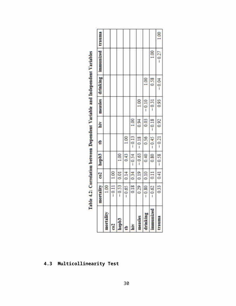
Before doing regression analysis, correlation analysis is conducted to check for the
relationship among all the variables. Then, a correlation matrix is also conducted for to
observe the correlations between variables. The correlation coefficient is a measure of
11
linear association between two variables. Values of the correlation coefficient are always
between -1 and +1. If a correlation coefficient of +1, it indicates that two variables are
perfectly related in a positive linear sense. If a correlation coefficient of -1, it indicates
that two variables are perfectly related in a negative linear sense; and if 0 indicates that
there is no linear relationship between the two variables.
3.2.2 Multiple Regression Analysis
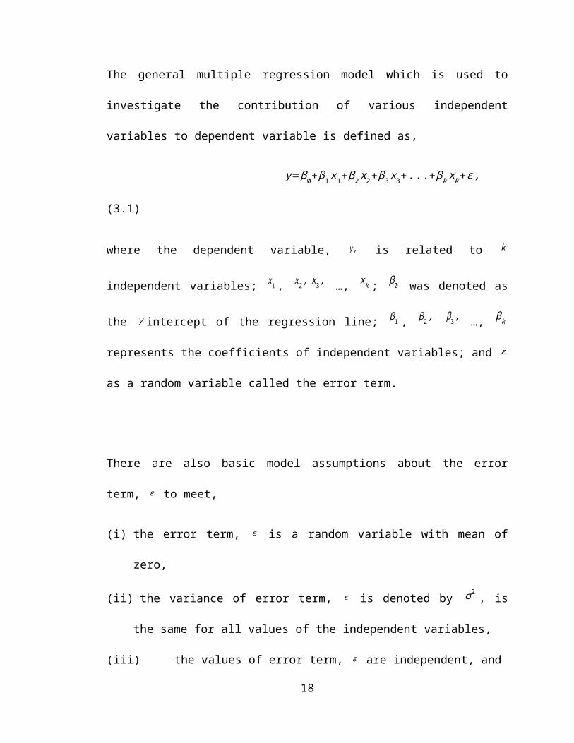
The general multiple regression model which is used to investigate the contribution of
various independent variables to dependent variable is defined as,
y=β0+β1 x1+ β2 x2+ β3 x3+.. .+βk xk+ε , (3.1)
where the dependent variable, y , is related to k independent variables; x1 , x2 , x3 , …,
xk ; β0 was denoted as the y intercept of the regression line; β1 , β2 , β3 , …, βk
represents the coefficients of independent variables; and ε as a random variable called
the error term.
There are also basic model assumptions about the error term, ε to meet,
12
(i) the error term, ε is a random variable with mean of zero,
(ii) the variance of error term, ε is denoted by σ2
, is the same for all values of the
independent variables,
(iii) the values of error term, ε are independent, and
(iv) the error term ε , is a normally distributed random variable.
OLS method is applied to illustrate the model that best characterizes the dataset of this
study, as well as to estimate the parameters.
3.2.3 Backward Elimination Technique
In the model selection phase of this Asian child mortality study, stepwise BE algorithm
is used. The BE technique starts by involving all the candidate independent variables
with calculating the F statistics in model, then deleting those variables one-by-one for
model improvement. This process is kept repeating until no improvement in the model is
possible. For BE methods, the default significant level in the statistical software SAS for
staying in the model is set as 0.15.
The details procedure in applying BE method are shown,
Step (a),
13
at the beginning, the original model is set as shown as Equation 3.1. Then, the following
k tests are carried out by setting the null hypothesis,
H0 j : β j=0 , j=1,2 ,. .. , k . (3.2)
The highest p-value which corresponding to
H0 l : β1=0 , (3.3)
is compared with the preselected significance p-value, which is 0.15.
Step 2(a), if p-value ¿ 0.15,
X l can be deleted and the new original model is
y=β0+β1 x1+ β2 x2+ β3 x3+.. .+β l−1 x l−1+β l+1 x l+1+. ..+βk xk +ε . (3.4)
Then, go back and repeat step 1.
Step 2(b), if p-value ¿ 0.15,
the original model is the model we should choose.
3.2.4 Data Transformation
14
To solve the potential modeling problems especially which caused by the violation of
assumptions while building a multiple regression model, a transformation in data is
needed to minimized or even fixed to improve the model accuracy.
A method which named as Box-Cox method is used to identify an appropriate
transformation on the response variable based on its set of independent variables.
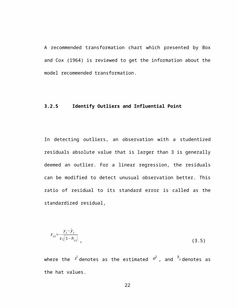
A recommended transformation chart which presented by Box and Cox (1964) is
reviewed to get the information about the model recommended transformation.
3.2.5 Identify Outliers and Influential Point
In detecting outliers, an observation with a studentized residuals absolute value that is
larger than 3 is generally deemed an outlier. For a linear regression, the residuals can be
modified to detect unusual observation better. This ratio of residual to its standard error
is called as the standardized residual,
r si=
y i− y i
s√(1−hii ) , (3.5)
where the s2
denotes as the estimated σ2
, and hii denotes as the hat values.
15
Then, studentized residual is further developed when estimate σ2
by s2( i ) , the estimate
σ 2is obtained after deleting the i
thobservation,
rti=
y i− y i
s( i)√1−hii . (3.6)
For indentifying influential data points in this study, difference in fits (DFITS) measure
is used. The basic idea of this measure is to delete each observation one-by-one, then
refitting the regression model on the remaining n−1 observation each time. Next, the
results using all the n observations to the results with the deleted ith
observation is
compared, and then it is able to see the influence impact on the analysis.
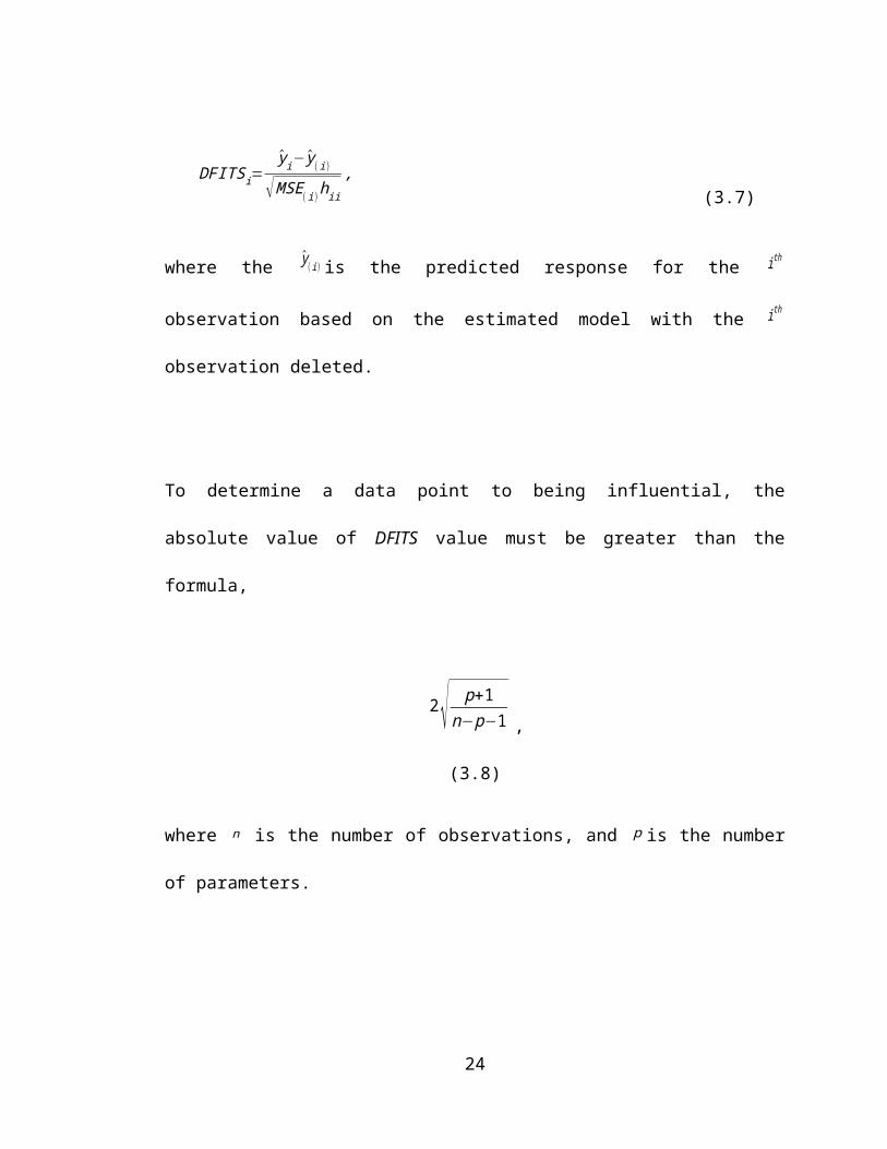
DFITSi for observation ith
is defined as,
DFITSi=
yi− y( i)
√ MSE( i)hii, (3.7)
where the y(i ) is the predicted response for the ith
observation based on the estimated
model with the ith
observation deleted.
16
To determine a data point to being influential, the absolute value of DFITS value must
be greater than the formula,
2√ p+1
n−p−1 , (3.8)
where n is the number of observations, and p is the number of parameters.
3.2.6 Robust Regression
Robust regression is a useful and important tool in analyzing a data set that
contaminated with outliers. While fitting a least squares regression, there might detect
some high leverage data points or outliers, and is confirmed not data entry errors. In this
situation, robust regression is a good strategy where it can be used in detecting outliers
and provided a stable results in presenting outliers. Robust regression also showed the
characteristics of weighted and reweighted least squares regression.
Basically, there are four methods under robust regression for the statistical applications
of outliers detection which are the M estimation, LTS estimation, S estimation, and MM
estimation. In my study, MM estimation is used due to this method is combining high
breakdown value estimation and the M estimation. Furthermore, it is able to achieve the
17
high breakdown point and perform higher statistical efficiency than S estimation
method.
CHAPTER 4
RESULTS AND DISCUSSION
4.1 Descriptive Statistics of the Data
There is a total of 8 independent variables and 47 observations in this study. For the
independent variables of co2, it is meant by the carbon dioxide emission which carried
the mean of 378354.47 metric tons per capita, standard deviation of 1249863.79, with a
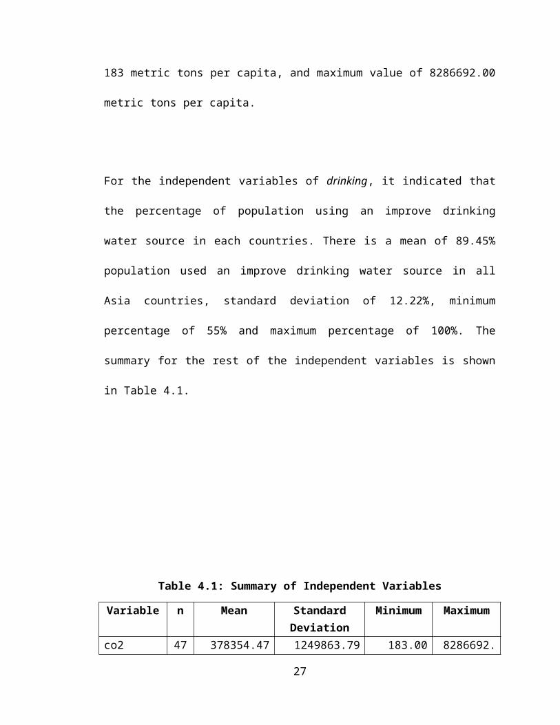
minimum value of 183 metric tons per capita, and maximum value of 8286692.00 metric
tons per capita.
For the independent variables of drinking, it indicated that the percentage of population
using an improve drinking water source in each countries. There is a mean of 89.45%
population used an improve drinking water source in all Asia countries, standard
18
deviation of 12.22%, minimum percentage of 55% and maximum percentage of 100%.
The summary for the rest of the independent variables is shown in Table 4.1.
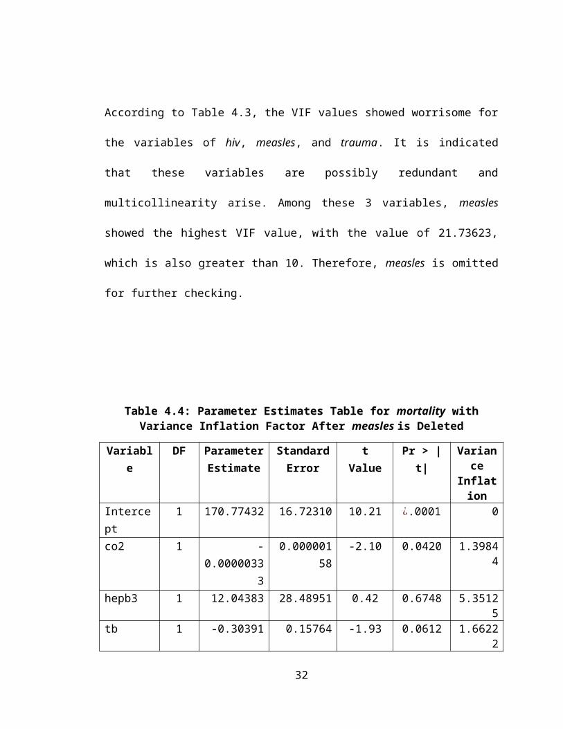
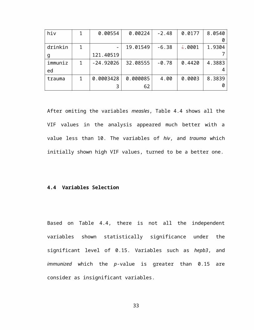
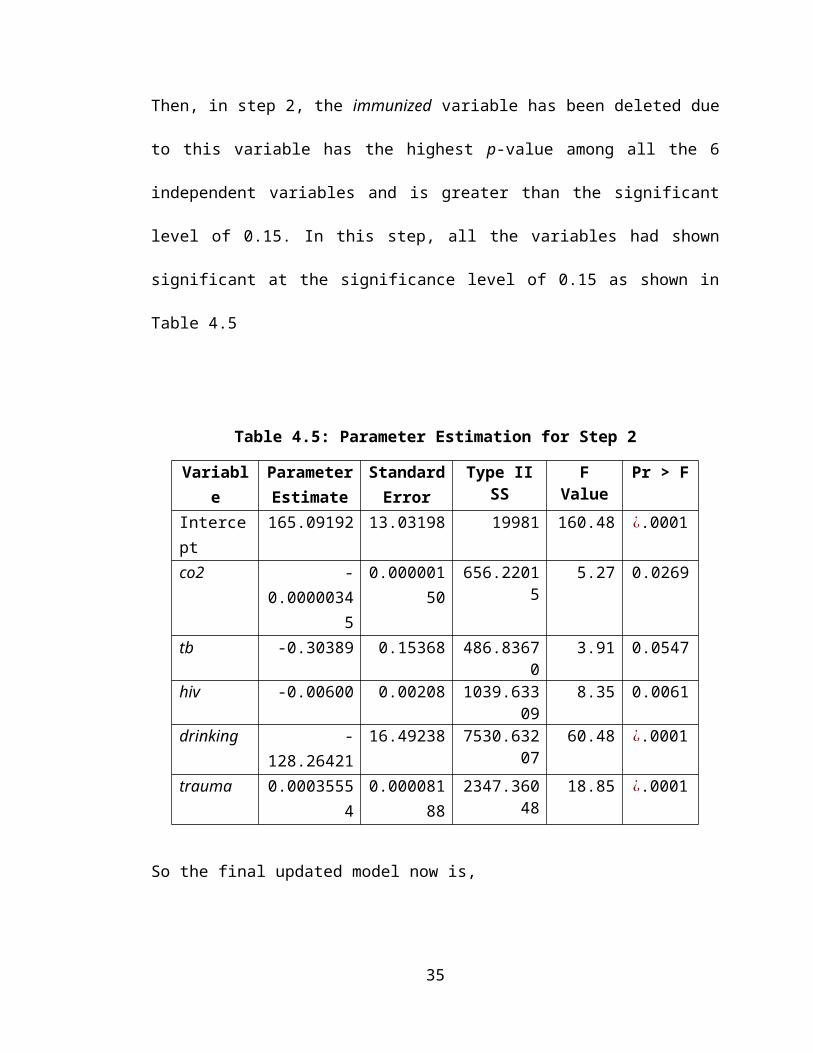
Note that, in this step 2, all the remaining variables which are co2, tb, hiv, drinking, and
trauma have the p-value less than 0.15. Therefore, the final reduced model is as shown
in Equation 4.1.
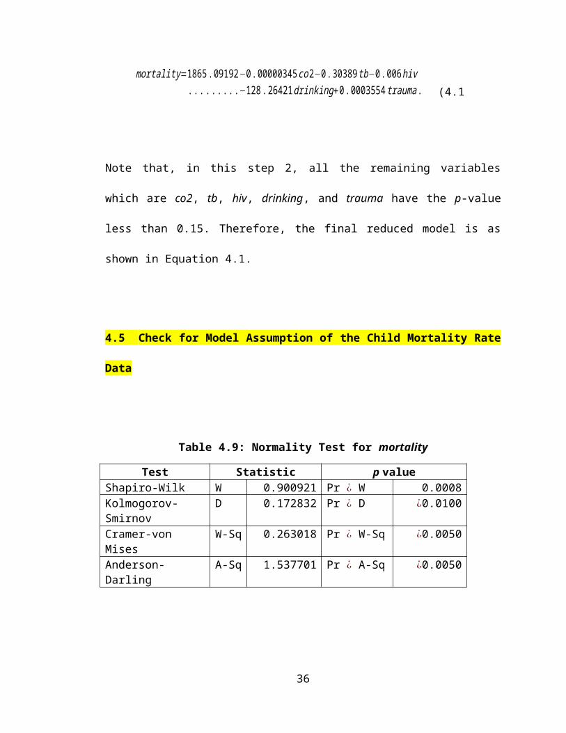
4.5 Check for Model Assumption of the Child Mortality Rate Data
Table 4.9: Normality Test for mortality
Test Statistic p valueShapiro-Wilk W 0.900921 Pr ¿ W 0.0008Kolmogorov-Smirnov D 0.172832 Pr ¿ D ¿0.0100Cramer-von Mises W-Sq 0.263018 Pr ¿ W-Sq ¿0.0050Anderson-Darling A-Sq 1.537701 Pr ¿ A-Sq ¿0.0050
25
(4.1)
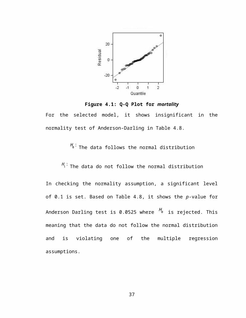
Figure 4.1: Q-Q Plot for mortality
For the selected model, it shows insignificant in the normality test of Anderson-Darling
in Table 4.8.
H0 : The data follows the normal distribution
H1 :The data do not follow the normal distribution
In checking the normality assumption, a significant level of 0.1 is set. Based on Table
4.8, it shows the p-value for Anderson Darling test is 0.0525 where H 0 is rejected. This
meaning that the data do not follow the normal distribution and is violating one of the
multiple regression assumptions.
Besides that, normality assumption also can be check through Q-Q plot as show in
Figure 4.1. It shown a linear trend with a slight deviation at the tail, this suggests that the
normality assumption is satisfied.
26
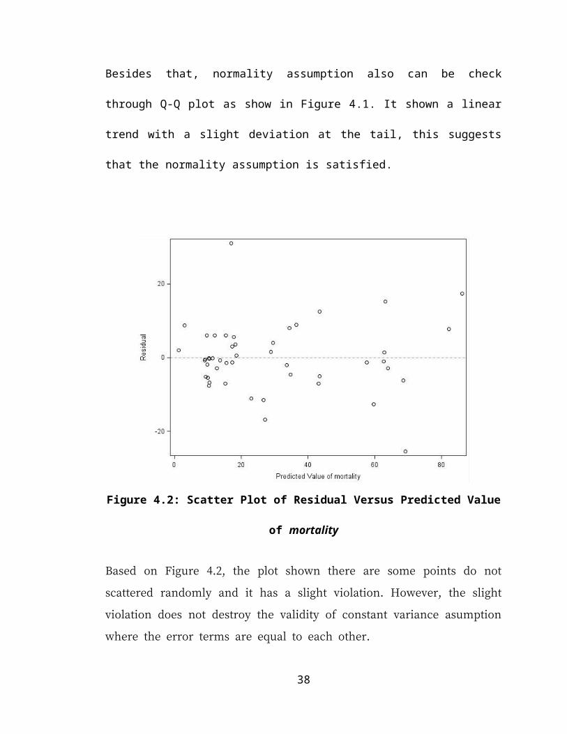
Figure 4.2: Scatter Plot of Residual Versus Predicted Value of mortality
Based on Figure 4.2, the plot shown there are some points do not scattered randomly and
it has a slight violation. However, the slight violation does not destroy the validity of
constant variance asumption where the error terms are equal to each other.
27
Figure 4.3: Scatter Plot of Residual Versus Regressors of mortality
By referring to Figure 4.3, there are 4 scatter plots shown which are residual versus to
the 4 selected independent variables such as co2, measles, drinking, and trauma. For all
the plots shown, they are not scattered randomly, and was scattered at one side.
Therefore, the linearity assumption is not valid in this mortality regression model.
From all the output shown, the regression model does not fulfill with multiple regression
assumptions, violation problem which may bring the model to be inefficient, seriosly
biased or misleading exited. So some apropriate statistical steps should take to overcome
this violation problem.
4.4 Data Transformation
28
To solve this violation assumptions problem, appropriate data transformation method is
needed in helping to minimize these violation problems. In this study a data
transformation method in making data to be normal is used which is based on Box and
Cox (1964). Their proposed on the recommended transformation table in referred.
According to the procedure developed, the λ value is indicating the power to which all
data should be raised. Therefore, the Box-Cox power transformation searches from
λ=−5 to λ =+ 5 until the best value is found.
Figure 4.4: Box-Cox Analysis for mortality
29
Based on Figure 4.4, the lambda value shown is 0.5 where according to the
recommended transformation table, the suggested transformation is to transform the
dependent variable, mortality to √mortality .
Table 4.10: Parameter Estimates Table for sqrtmortality
After a transformation is done, according to Table 4.9, the regression analysis showed
all the selected variables through BE search algorithm is statistically significance at the
significant level set. Furthermore, in Table 4.9 also showed all the estimated regression
coefficients have different values as shown in Table 4.7 which the regression analysis is
done before the transformation is done.
For the assumption checking process is needed to check there is no assumptions
violation problem on the data of this child mortality rate study. When there are any
assumptions which stated in Section 3.2.2 is violated, then the predictions and
confidence intervals by a regression model maybe inefficient, seriously biased or even
causes misleading.
30
According to the previous normality test before data transformation is done, the data
shown the error distribution is significantly non-normal. Therefore, Box-Cox
transformation method is used to overcome this violation problem.
Table 4.11: Normality Test for sqrtmrtality
Test Statistic p valueShapiro-Wilk W 0.951442 Pr ¿ W 0.0835Kolmogorov-Smirnov D 0.10437 Pr ¿ D ¿ 0.1500Cramer-von Mises W-Sq 0.124595 Pr ¿ W-Sq 0.1941Anderson-Darling A-Sq 0.733602 Pr ¿ A-Sq 0.1953
According to Table 4.10, it is statistical significance in the normality test of Anderson-
Darling for the regression model after the transformation data is done.
H0 : The data follows the normal distribution
H1 :The data do not follow the normal distribution
In checking the normality assumption, a significant level of 0.1 is set. Based on Table
4.10, it shows the p-value for Anderson Darling test is 0.1953 where H0 is fail to reject.
This meaning that the child mortality rate data follow the normal distribution.
31
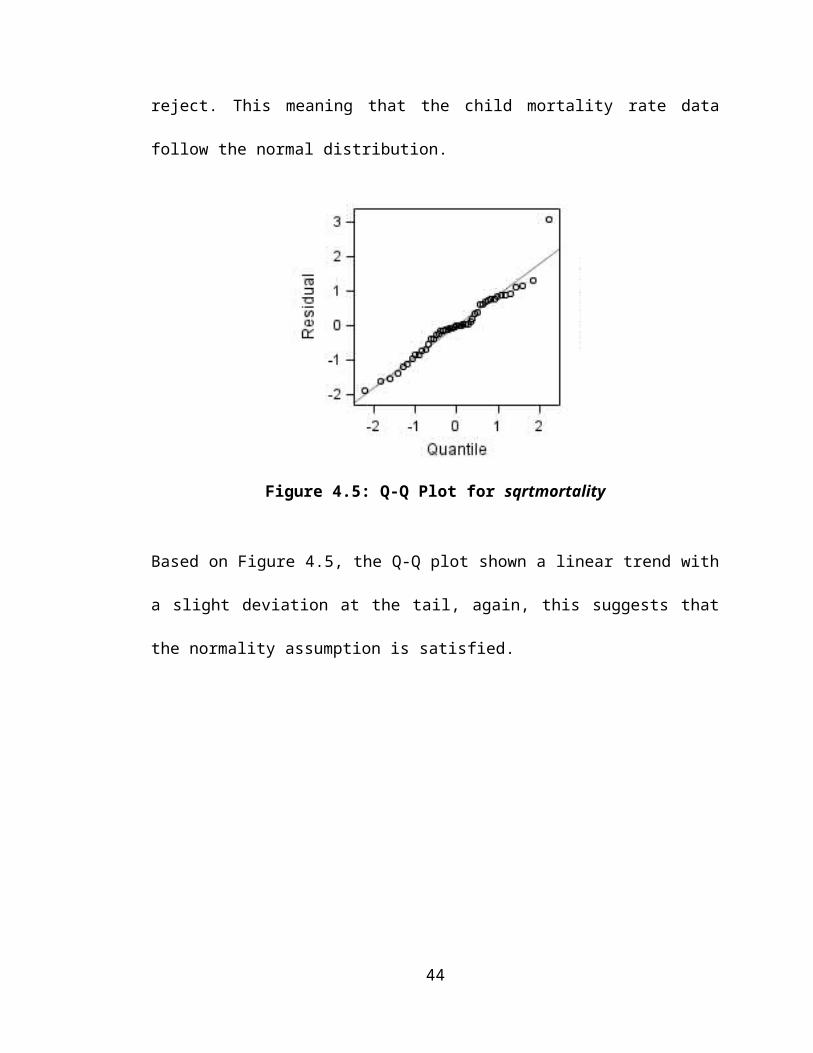
Figure 4.5: Q-Q Plot for sqrtmortality
Based on Figure 4.5, the Q-Q plot shown a linear trend with a slight deviation at the tail,
again, this suggests that the normality assumption is satisfied.
Figure 4.6: Scatter Plot of Residual Versus Predicted Value of sqrtmortality
32
Based on Figure 4.6, the plot shown there are some points do not scattered randomly and
it has a slight violation. However, the slight violation does not destroy the validity of
constant variance asumption where the error terms are equal to each other.
Figure 4.7: Scatter Plot of Residual Versus Regressors of sqrtmortality
By referring to Figure 4.7, there are 4 scatter plots shown which are residual versus to
the 4 selected independent variables such as co2, measles, drinking, and trauma. For all
the plots shown, they are not scattered randomly, and was scattered at one side.
Therefore, the linearity assumption is not valid in this sqrtmortality regression model.
33
Figure 4.8: Scatter Plot of Studentized Residual Versus Leverage
Since the data transformation method yet to overcome the assumption violation problem,
and there is also presence of potential outliers, influential points and high leverage point
as shown in Figure 4.8. Therefore, Robust Regression is used to obtain a fit that is
resistant to the presence of high leverage points and outliers.
4.5 Indentifying Outliers and Influential Points
4.5.1 Outliers Determination
Outliers are referring to a data point which its response y does not follow the general
trend of the data, or in other words, it is an observation point that us distant from other
observations. Influential point is a data point which it is immoderately influencing any
34
part of a regression analysis, such as the predicted responses, the estimated slope
coefficients, or the hypothesis test result. In this study, there are few data points shown
the potential characteristics of outliers and influential points.
Figure 4.9: Scatter Plot of Studentized Residual Versus Predicted Value of sqrtmortality
Figure 4.9 gave evidence of the presence of outlying observations, it shown there are 2
points fall behind the band. In order to identify which data points are the outliers, an
observation with a studentized residuals absolute value that is larger than 3 is generally
deemed an outlier.
Table 4.12: Studentized Residuals Absolute Value Larger Than 3
Observation Country Studentized Residual6 Bhutan 3.308878 Cambodia -2.13049
35
Table 4.11 showed the 2 highest absolute studentized residual values among the 47
observations. However, there is only one observation shown its absolute value greater
than 3. Therefore, only observation 6, which is Bhutan is identified as the outlier.
The reason behind of the child mortality rate in Bhutan has a vary observation compared
to other Asia countries may cause by there was a flash floods from major rivers in May
2009. According to Central Intelligence Agency (CIA) World Factbook (2012), this
flash floods been caused major destruction to lives and properties, as well as the many
death cases been reported.
Furthermore, the Bhutan newly elected government in year 2009 just began to focus a
program named by Early Childhood Care and Education (ECCD) which focus on
enhancing the development of Bhutan children, prepare them to school, and to overcome
children basic health problem in year 2010. This late action also might cause the child
mortality rate in Bhutan to be different.
4.5.2 Influential Points Determination
To identify influential point in this child under age of five mortality study, DFITS
measure is used. Therefore, any absolute DFITS values greater than
2√ 5+1
47−5−1=0 .7651
, (4.6)
36
are consider as influential data points.
Table 4.13: Absolute DFITS Values Lager than 0.7651
Observation Country DFITS Value8 Cambodia -0.7963812 India -3.69008
Table 4.12 shown that there are 2 influential data points in this study which are
Cambodia with just a slight influencing and India which playing the most influencing
role to the data. This is not surprise, as India has the biggest population and the highest
child mortality rate in the region of Asia.
4.6 Robust Regression
Since there are still outliers and influential points detected even the data had been
transformed. Therefore, robust regression with MM method which able to obtain a fit
that is resistant to the presence of outliers and influential data points is used in this study.
Hence, the estimated regression coefficients are compared between robust regression
and OLS regression.
37
All of the independent variables are tested in robust regression at first and the highest p-
value which greater than significant level, 0.15 is deleted each time. The insignificant
variables are deleted one-by-one until only those significant variables are remained in
Table 4.17 shown that all the estimated regression coefficients have different value, as
well as the number of significance parameters have been increasing from 4 variables to 5
variables in the OLS regression and robust regression respectively.
The difference observed is due to robust regression which able to obtain a fit that is
resistant to the presence of outliers and influential data points. Robust regression is a
design which not overly affected by assumptions violations whereas OLS can give
misleading result when there are any violation problems. Therefore, the result of
estimated regression coefficients for robust regression is believe to be more accurate
compared with the result from OLS regression.
CHAPTER 5
41
CONCLUSION AND FUTURE WORK
5.1 Conclusion
The findings of this study reveal that the main determinants affecting child under age of
five mortality rate in Asia countries are carbon dioxide emission, case detection rate for
all forms of tuberculosis, number of reported deaths on measles, population using an
improved drinking water source, children immunized against measles, and number of
birth trauma reported. These 5 independent variables have statistically significant
impacts on the dependent variables.
Bhutan where occurred a flash flood in May 2009 caused major destroyed and death in
this country, hence it was shown that Bhutan has a different child mortality observation
compared to other countries in Asia. India, one of the countries which has the biggest
population and highest mortality rate in Asia, it showed that it has a characteristic of
influencing to this study.
Children are the future leader of a country. They the group of people who we need to
protect the most to make sure they have a healthy environment to survive, to grow up.
Then only they are able to lead the country to a brighter future. Government of each
Asia countries should come out with a rules or guidelines to improve the living quality
42
of children, to let all the children are live healthy and safely. Moreover, regional
cooperation among the Asia communities should be included to overcome this child
mortality problem, and reduce the case to minimum.
5.2 Future Work
In the future, this child mortality rate analysis can be carried out by using the method of
robust regression with other estimation such as the M estimation, LTS estimation or S
estimation.
Besides that, more factors which may cause child mortality in Asia can also be in
included in the further analysis in future. The example of factors such as the income
group, gross domestic product (GDP), cases of child malnutrition, underweight are
suggested to use in the analysis of child mortality in Asia.
REFERENCES
43
Aiken, L. S., West, S. G. and Pitts, S. C. Multiple Linear Regression in Handbook of Psychology ed. Schinka, J. A., Velicer, W. F. and Weiner, I. B. Canada: John Wiley & Sons Inc., 2003.
Bianco, A. M., Ben, M. G. and Yohai, V. J. 2005. Robust Estimation for Linear Regression with Asymmetric Errors, Canadian Journal of Statistics. 33: 511-528.
Black, R. E., Morris, S. S. and Bryce, J. 2003. Where and Why are 10 Million Children Dying Every Year, The Lancet. 361: 2226-2234.
Box, G. E. P., and Cox, D. R. 1964. An Analysis of Transformations, Journal Royal Statistics Society, Series B. 26: 211-234.
Broadhurst, D., Goodacre, R., Jones, A., Rowland, J. J. and Kell, D. B. 1996. Genetic Algorithms as a Method for Variable Selection in Multiple Linear Regression and Partial Least Squares Regression, with Applications to Pyrolysis Mass Spectrometry, Analytica Chimica Acta. 348: 71-86.
Chatterjee, S. and Hadi, A.S. 1986. Influential Observations, High Leverage Points, and Outliers in Linear Regression, Statistical Science. 1: 379-416.
Draper, N. R. and Smith, H. Applied Regression Analysis 2nd Edition: John Wiley and Sons, New York, 1981.
Gabriele, A. and Schettino, F. 2008. Child Malnutrition and Mortality in Developing Countries: Evidence from a Cross-Country Analysis, Analysis of Social Issue and Public Policy. 8: 53-81.
Grossman, Y. L., Ustin, S. L., Jacquemoud, S., Sanderson, E. W., Schmuck, G. and Verdebout, J. 1996. Critique of Stepwise Multiple Linear Regression for the Extraction of Leaf Biochemistry Information from Leaf Reflectance Data, Remote Sensing of Environment. 56: 182-193.
44
Hall, R., Fienberg, S. E. and Nardi, Y. 2011. Secure Multiple Linear Regression Based on Homomorphic Encrption, Journal of Official Statistics. 27: 1-23.
Huber, P. J. 1973. Robust Regression: Asymptotics, Conjectures and Monte Carlo, Ann. Stat., 1: 799-821.
Maronna R. A. and Yohai, V. J. 2013. Robust Functional Linear Regression Based on Splines, Computational Statistics & Data Analysis. 65: 46-55.
Quinino, R. C., Reis, E. A. and Bessegato, L. F. 2011. Using the Coefficient of Determination R2 to Test the Significance of Multiple Linear Regression, Teaching Statistics. 35: 84-88.
Rousseeuw, P. J. 1984. Least Median of Squares Regression, Journal of the American Statistical Association, 79: 871-880.
Rousseeuw, P. J. and Yohai, V. Robust Regression by Means of S Estimatiors in Robust and Nonlinear Time Series Analysis ed. Franke, J., Härdle W. and Martin, R. D. New York: Springer Verlag, 1984.
Sarmin, M., Ahmed, T., Bardhan, P. K. and Chisti, M. J. 2014. Specialist Hospital Study Shows that Septic Shock and Drowsiness Predict Mortality in Children Under Five with Diarrhoea, Acta Paediatrica. 1-6.
Telmo, C., Lousada, J. and Moreira, N. 2010. Proximate Analysis, Backward Stepwise Regression Between Gross Calorific Value, Ultimate and Clinical Analysis of Wood, Bioresource Technology. 101: 3808-3815.
45
Yohai, V. J. 1987. High Breakdown Point and High Efficiency Robust Estimates for Regression, Annals of Statistics. 15: 642-656.
Zainodin, H. J., Noraini, A. and Yap, S. J. 2011. An Alternative Multicollinearity Approach in Solving Multiple Regression Problem, Trends in Applied Sciences Research. 6: 1241-1255.