MLSP2012 Tutorial: Manifold Learning: Modeling and Algorithms Dr. Raviv Raich (presenting) Behrouz Behmardi School of Electrical Engineering and Computer Science Oregon State University, Corvallis, OR 97331-5501
Transcript
MLSP2012 Tutorial:
Manifold Learning: Modeling and
Algorithms
Dr. Raviv Raich (presenting)
Behrouz Behmardi
School of Electrical Engineering and Computer Science
Oregon State University, Corvallis, OR 97331-5501
Acknowledgment
• Behrouz Behmardi, PhD candidate,
Oregon State University
• Dr. Alfred Hero, Prof. EECS, University
of Michigan
• Dr. Kevin Carter, Lincoln Labs
• Dr. Steve Damelin, Prof. math.
Outline
• Motivation
• Mathematical Background
– Linear models and algorithms
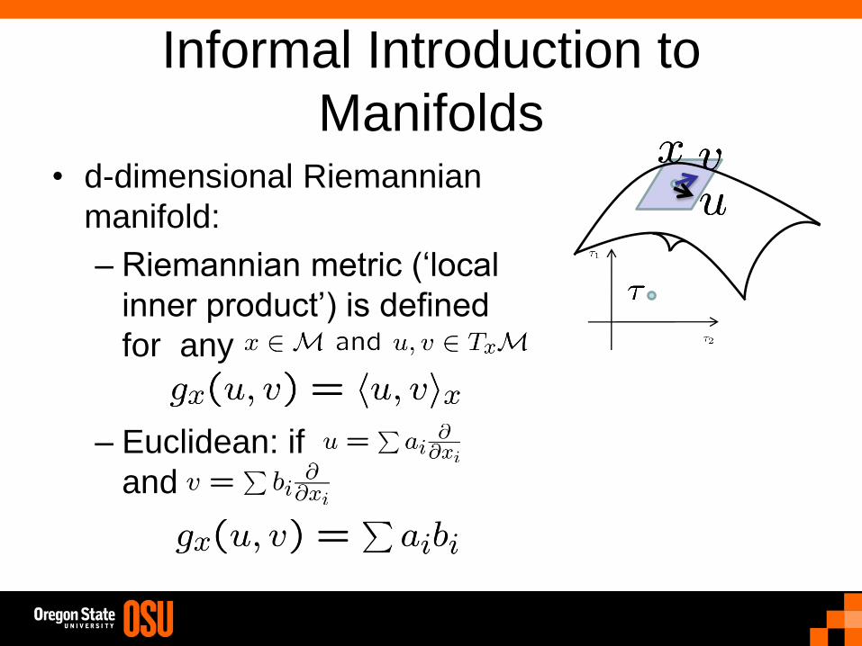
– Manifolds (terminology)
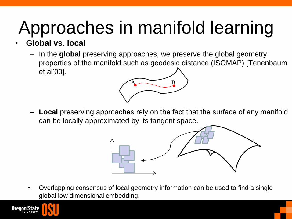
• Manifold learning approaches
– Geometric
– Probabilistic
• New directions
Motivation
• Large volume, high dimensional data
• Dimension reduction for:
– Visualization: insight into the dataset
– Compression: storage
– Denoising: remove redundant dimensions,
reduce classifier complexity = improve
generalization
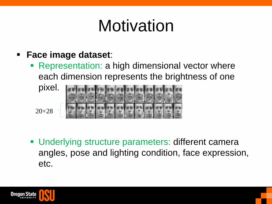
Motivation
Face image dataset:
Representation: a high dimensional vector where
each dimension represents the brightness of one
pixel.
Underlying structure parameters: different camera
angles, pose and lighting condition, face expression,
etc.
20×28
Motivation
Character recognition:
Representation: a high dimensional vector where
each dimension represents the brightness of one
pixel.
Underlying structure parameters: orientation,
curvature, style (e.g., 2 with/without loops )
28×28
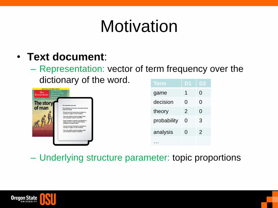
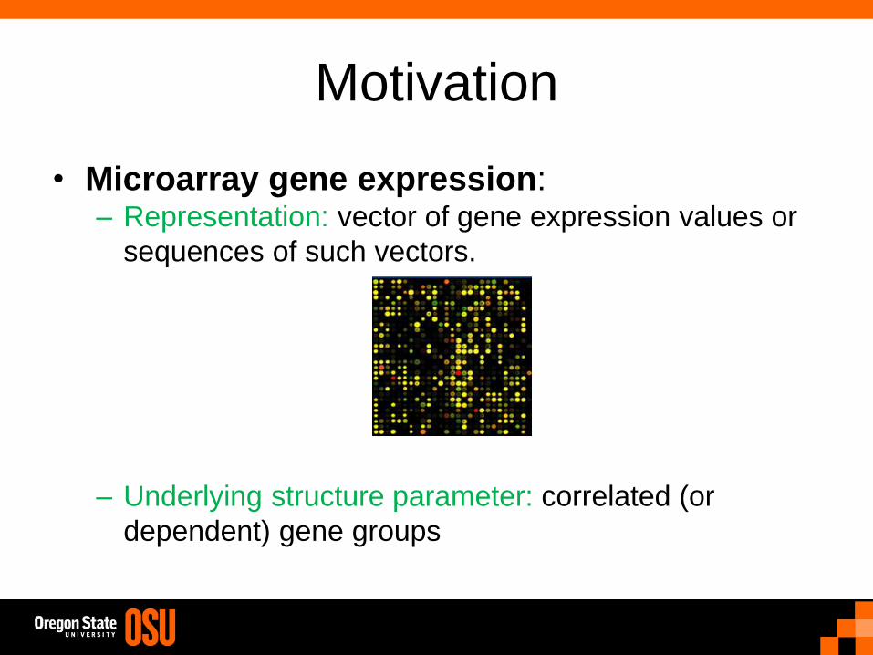
Motivation
• Text document: – Representation: vector of term frequency over the
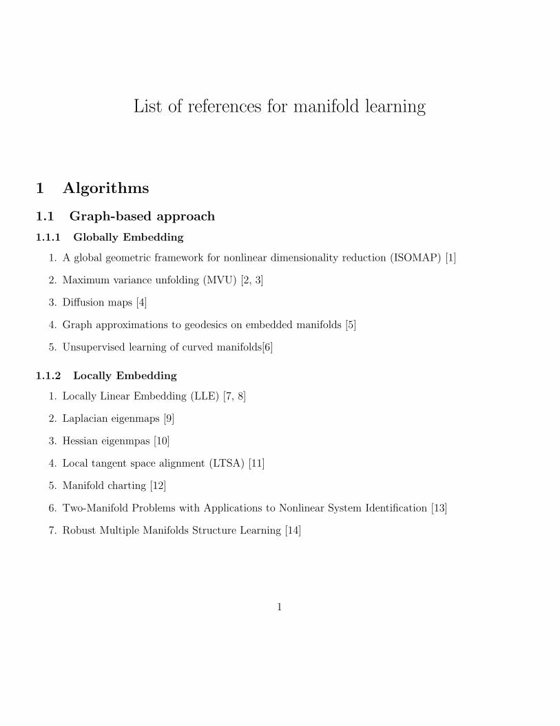
2. Graph laplacian regularization for large-scale semidefinite programming [16]
3. Modified locally linear embedding [17]
4. Colored maximum variance unfolding [18]
5. Grouping and dimensionality reduction by locally linear embedding [19]
6. Sparse multidimensional scaling using landmark points [20]
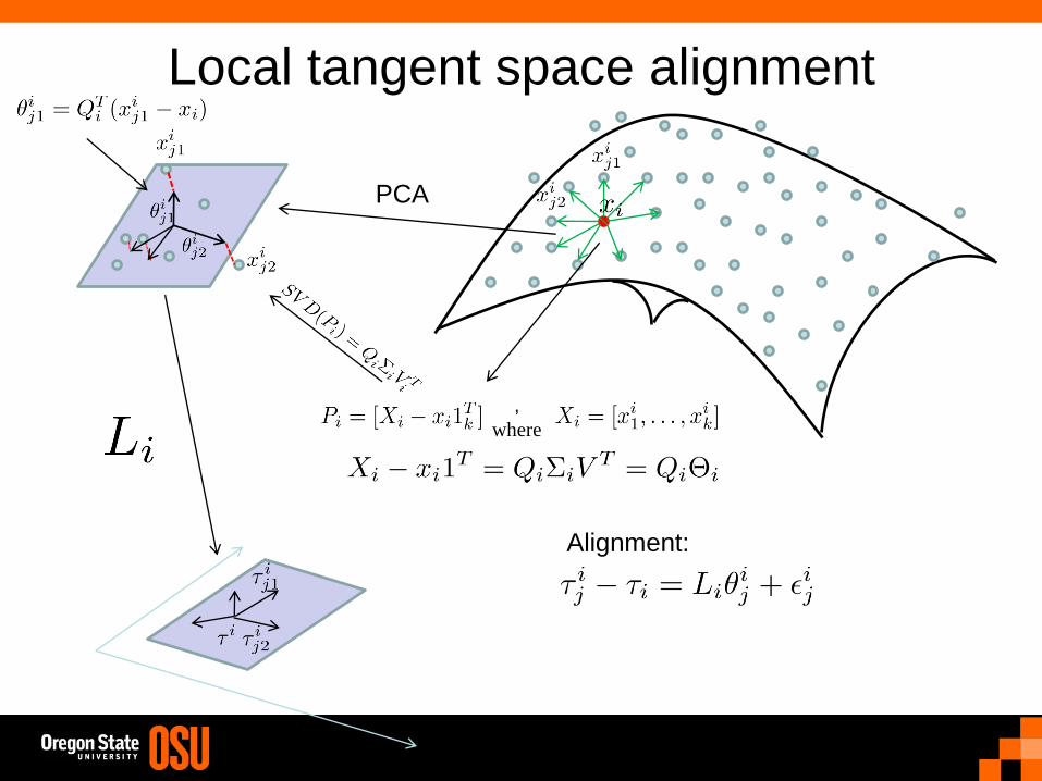
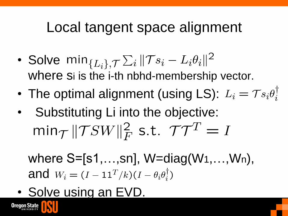
7. Improved local coordinate coding using local tangents [21]
1.2 Probabilistic approach
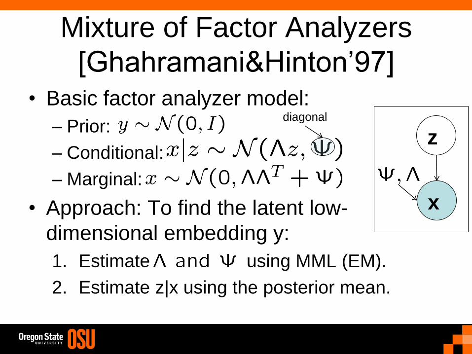
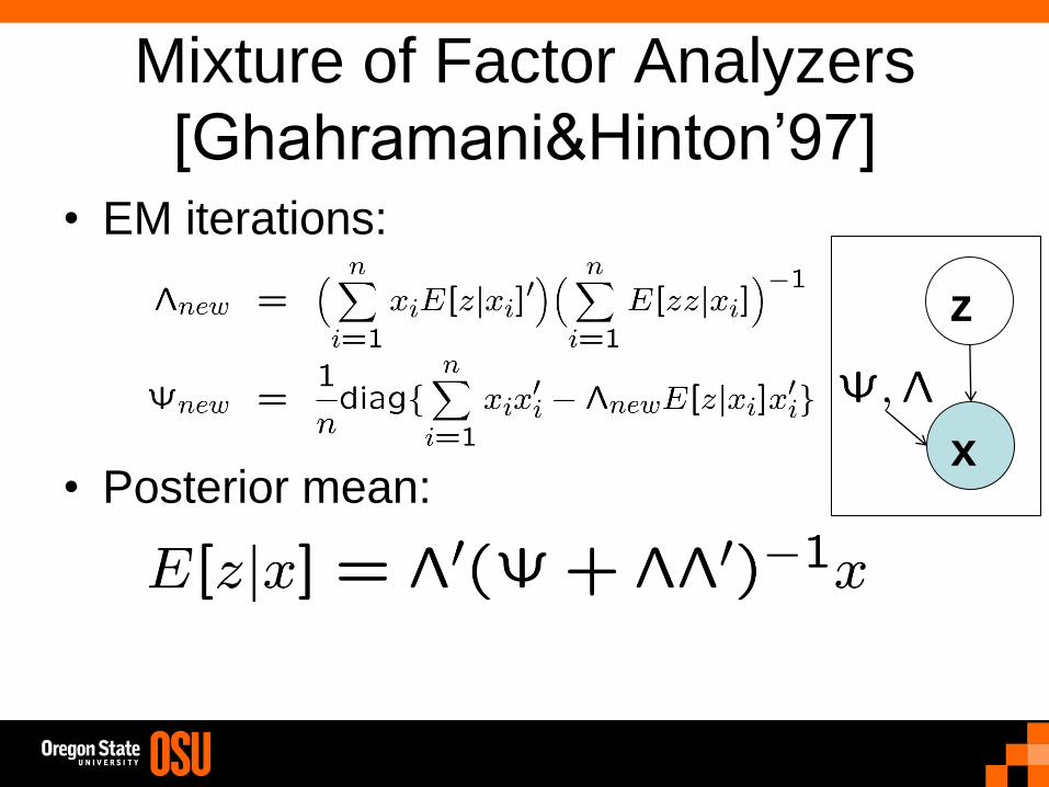
1. Mixture of factor analysis (MFA) [22]
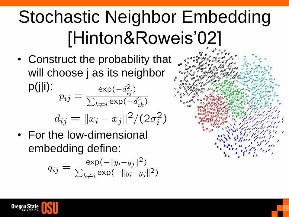
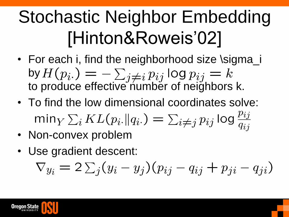
2. Stochastic neighborhood embedding (SNE) [23]
3. The generative topographic mapping (GTM) [24]
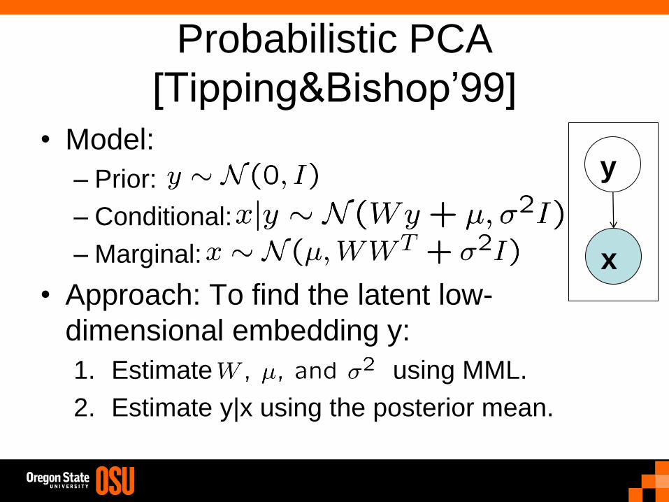
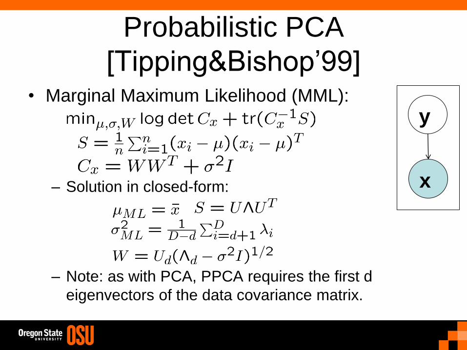
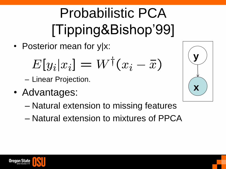
4. Probabilistic principal component analysis [25]
5. Global coordinate of local linear models [26]
6. Automatic alignment of local representations [27]
7. Coordinating principal component analysis [28]
1.3 Non-probabilistic approach
1. Multilayer autoencoders [29]
2. The self-organizing map [30]
3. Sammon mapping [31]
4. Kernel PCA [32]
5. Principal curves [33]
6. A variational approach to recovering a manifold from sample points [34]
2
7. Out-of-sample extensions for LLE, Isomap, MDS, Eigenmaps, and spectral clustering [35]
8. Continuous nonlinear dimensionality reduction by kernel eigenmaps [36]
9. Learning eigenfunctions links spectral embedding and kernel PCA [37]
10. Sparse manifold clustering and embedding [38]
1.4 Supervised and semisupervised manifold learning
1. Vector-valued manifold regularization [39]
2. Multiple instance learning with manifold bags [40]
3. The manifold tangent classifier [41]
2 Applications
1. Maximum covariance unfolding: Manifold learning for bimodal data [42]
2. Humans learn using manifolds, reluctantly [43]
3. Learning multiple tasks using manifold regularization [44]
4. Online learning in the manifold of low-rank matrices [45]
5. Manifold Precis: An Annealing Technique for Diverse Sampling of Manifolds [46]
6. Nonlinear dimensionality reduction as information retrieval [47]
7. Information retrieval perspective to nonlinear dimensionality reduction for data visualization [48]
8. Unified Locally Linear Embedding and Linear Discriminant Analysis Algorithm (ULLELDA) forFace Recognition [49]
9. Generative modeling for continuous non-linearly embedded visual inference [50]
10. Manifold learning and applications in recognition [51]
11. Graph-driven features extraction from microarray data using diffusion kernels and kernel CCA [52]
12. Manifold based analysis of facial expression [53]
13. A dimensionality reduction approach to modeling protein flexibility [54]
3
14. Face recognition from face motion manifolds using robust kernel resistor-average distance [55]
15. Coloring of DT-MRI fiber traces using Laplacian eigenmaps [56]
16. Freeway traffic stream modeling based on principal curves and its analysis [57]
17. Super-resolution through neighbor embedding [58]
3 Dimension Estimation
1. Manifold-adaptive dimension estimation [59]
2. Towards manifold-adaptive learning [60]
3. Maximum likelihood estimation of intrinsic dimension [61]
4. Manifold learning using Euclidean k-nearest neighbor graphs [62]
5. An intrinsic dimensionality estimator from near-neighbor information [63]
6. Intrinsic dimension estimation of manifolds by incising balls [64]
7. Intrinsic dimension estimation by maximum likelihood in probabilistic PCA [65]
References
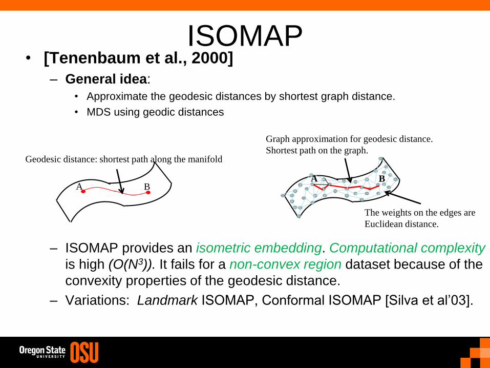
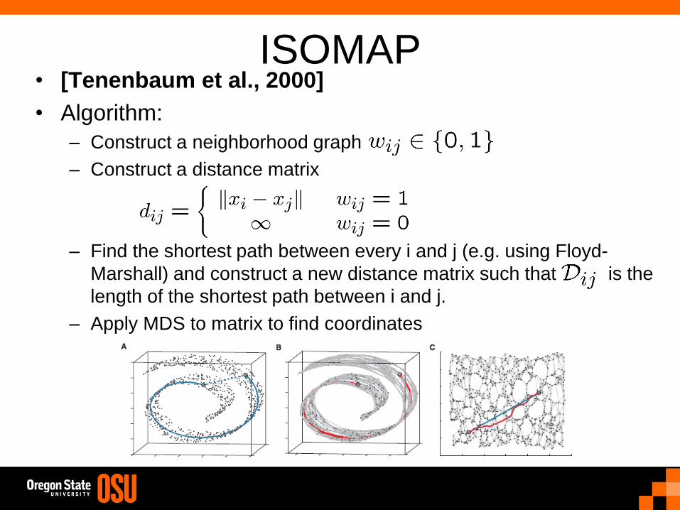
[1] J.B. Tenenbaum, V. De Silva, and J.C. Langford, “A global geometric framework for nonlineardimensionality reduction,” Science, vol. 290, no. 5500, pp. 2319–2323, 2000.
[2] K.Q. Weinberger and L.K. Saul, “Unsupervised learning of image manifolds by semidefinite pro-gramming,” in Computer Vision and Pattern Recognition, 2004. CVPR 2004. Proceedings of the2004 IEEE Computer Society Conference on. IEEE, 2004, vol. 2, pp. II–988.
[3] K.Q. Weinberger, F. Sha, and L.K. Saul, “Learning a kernel matrix for nonlinear dimensionalityreduction,” in Proceedings of the twenty-first international conference on Machine learning. ACM,2004, p. 106.
[4] R.R. Coifman and S. Lafon, “Diffusion maps,” Applied and Computational Harmonic Analysis, vol.21, no. 1, pp. 5–30, 2006.
[5] M. Bernstein, V. De Silva, J.C. Langford, and J.B. Tenenbaum, “Graph approximations to geodesicson embedded manifolds,” Tech. Rep., Technical report, Department of Psychology, Stanford Uni-versity, 2000.
4
[6] V. de Silva and J. Tenenbaum, “Unsupervised learning of curved manifolds,” in Proceedings of theMSRI workshop on nonlinear estimation and classification, 2002.
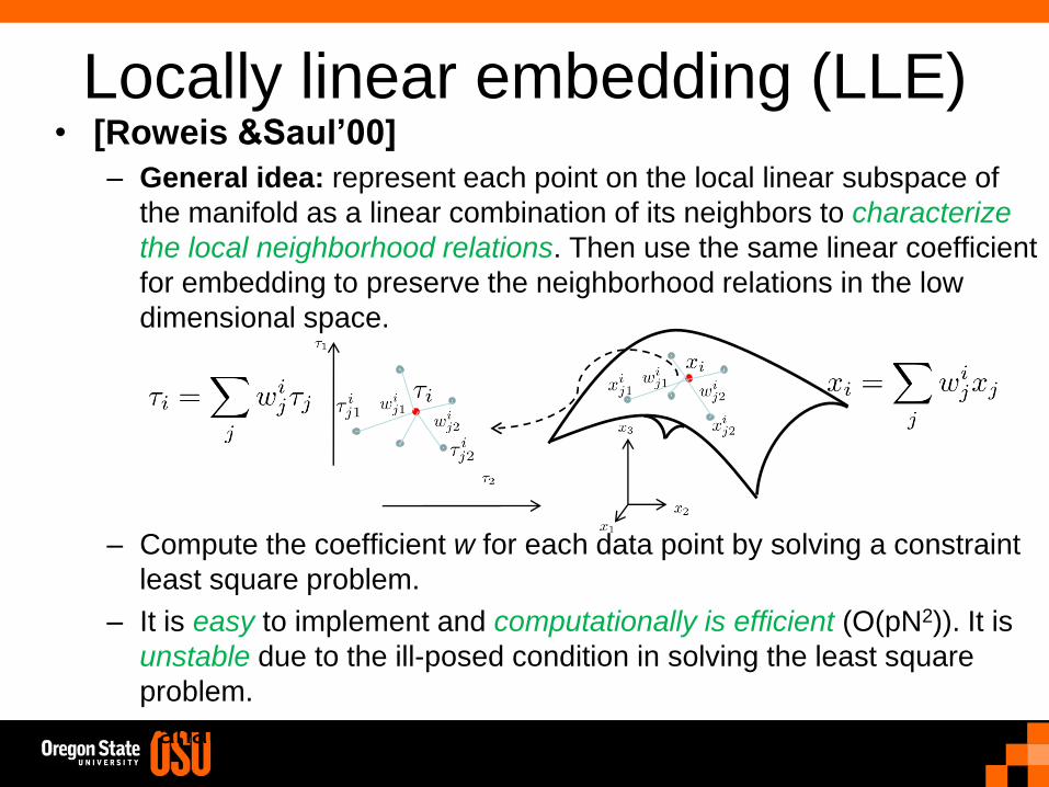
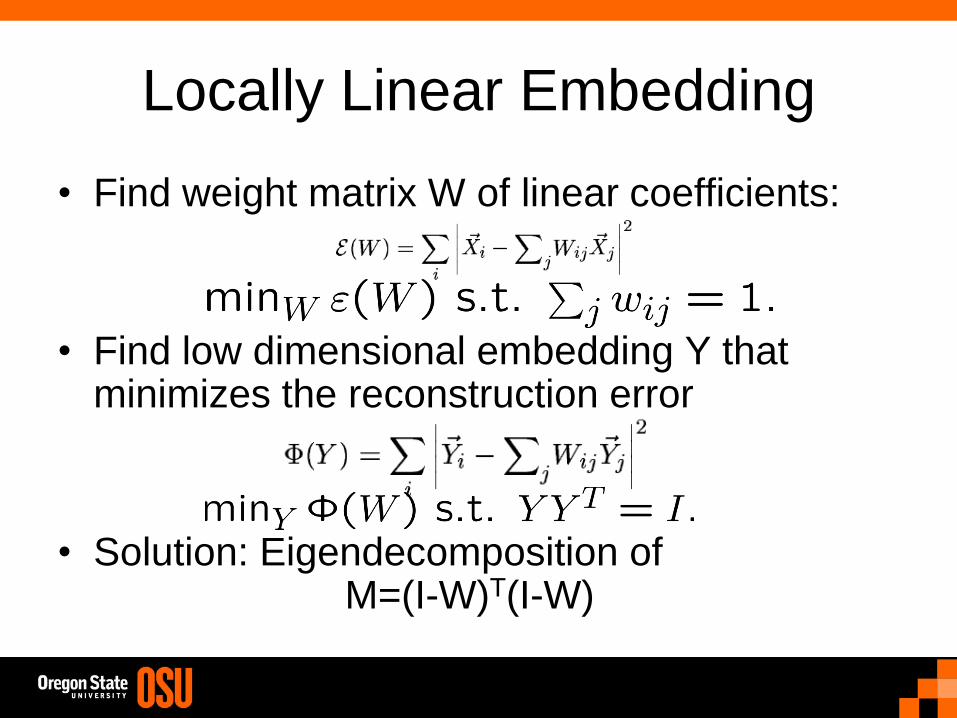
[7] S.T. Roweis and L.K. Saul, “Nonlinear dimensionality reduction by locally linear embedding,”Science, vol. 290, no. 5500, pp. 2323–2326, 2000.
[8] L.K. Saul and S.T. Roweis, “An introduction to locally linear embedding,” unpublished. Availableat: http://www. cs. toronto. edu/˜ roweis/lle/publications. html, 2000.
[9] M. Belkin and P. Niyogi, “Laplacian eigenmaps and spectral techniques for embedding and cluster-ing,” Advances in neural information processing systems, vol. 14, pp. 585–591, 2001.
[10] D.L. Donoho and C. Grimes, “Hessian eigenmaps: Locally linear embedding techniques for high-dimensional data,” Proceedings of the National Academy of Sciences of the United States of America,vol. 100, no. 10, pp. 5591, 2003.
[11] T. Zhang, J. Yang, D. Zhao, and X. Ge, “Linear local tangent space alignment and application toface recognition,” Neurocomputing, vol. 70, no. 7, pp. 1547–1553, 2007.
[12] M. Brand, “Charting a manifold,” Advances in neural information processing systems, pp. 985–992,2003.
[13] B. Boots and G. Gordon, “Two-manifold problems with applications to nonlinear system identifica-tion,” ICML2012, 2012.
[14] D. Gong, X. Zhao, and G. Medioni, “Robust multiple manifolds structure learning,” ICML2012,2012.
[15] V. Silva and J.B. Tenenbaum, “Global versus local methods in nonlinear dimensionality reduction,”Advances in neural information processing systems, vol. 15, pp. 705–712, 2003.
[16] K.Q. Weinberger, F. Sha, Q. Zhu, and L.K. Saul, “Graph laplacian regularization for large-scalesemidefinite programming,” Advances in neural information processing systems, vol. 19, pp. 1489,2007.
[17] Z. Zhang and J. Wang, “Mlle: Modified locally linear embedding using multiple weights,” Advancesin Neural Information Processing Systems, vol. 19, pp. 1593, 2007.
[18] L. Song, A. Smola, K. Borgwardt, and A. Gretton, “Colored maximum variance unfolding,” Advancesin neural information processing systems, vol. 20, pp. 1385–1392, 2008.
[19] M. Polito and P. Perona, “Grouping and dimensionality reduction by locally linear embedding,”Advances in Neural Information Processing Systems, vol. 14, pp. 1255–1262, 2001.
5
[20] V. De Silva and J.B. Tenenbaum, “Sparse multidimensional scaling using landmark points,” Tech-nology, pp. 1–41, 2004.
[21] K. Yu and T. Zhang, “Improved local coordinate coding using local tangents,” in Proc. of the IntlConf. on Machine Learning (ICML), 2010.
[22] Z. Ghahramani and G.E. Hinton, “The em algorithm for mixtures of factor analyzers,” Tech. Rep.,Technical Report CRG-TR-96-1, University of Toronto, 1996.
[23] G. Hinton and S. Roweis, “Stochastic neighbor embedding,” Advances in neural information pro-cessing systems, vol. 15, pp. 833–840, 2002.
[24] C.M. Bishop, M. Svensen, and C.K.I. Williams, “Gtm: The generative topographic mapping,”Neural computation, vol. 10, no. 1, pp. 215–234, 1998.
[25] M.E. Tipping and C.M. Bishop, “Probabilistic principal component analysis,” Journal of the RoyalStatistical Society: Series B (Statistical Methodology), vol. 61, no. 3, pp. 611–622, 1999.
[26] ST Roweis, L.K. Saul, and G.E. Hinton, “Global coordination of local linear models,” Advances inneural information processing systems, vol. 2, pp. 889–896, 2002.
[27] Y.W. Teh and S. Roweis, “Automatic alignment of local representations,” Advances in neuralinformation processing systems, vol. 15, pp. 841–848, 2002.
[28] J. Verbeek, N. Vlassis, and B. Krose, “Coordinating principal component analyzers,” ArtificialNeural NetworksICANN 2002, pp. 140–140, 2002.
[29] D. DeMers and G. Cottrell, “Non-linear dimensionality reduction,” Advances in neural informationprocessing systems, pp. 580–580, 1993.
[30] T. Kohonen, “The self-organizing map,” Proceedings of the IEEE, vol. 78, no. 9, pp. 1464–1480,1990.
[31] J.W. Sammon Jr, “A nonlinear mapping for data structure analysis,” Computers, IEEE Transactionson, vol. 100, no. 5, pp. 401–409, 1969.
[32] B. Scholkopf, A. Smola, and K.R. Muller, “Kernel principal component analysis,” Artificial NeuralNetworksICANN’97, pp. 583–588, 1997.
[33] T. Hastie and W. Stuetzle, “Principal curves,” Journal of the American Statistical Association, pp.502–516, 1989.
[34] J. Gomes and A. Mojsilovic, “A variational approach to recovering a manifold from sample points,”Computer VisionECCV 2002, pp. 3–17, 2002.
6
[35] Y. Bengio, J.F. Paiement, P. Vincent, O. Delalleau, N. Le Roux, and M. Ouimet, “Out-of-sampleextensions for lle, isomap, mds, eigenmaps, and spectral clustering,” Advances in neural informationprocessing systems, vol. 16, pp. 177–184, 2004.
[36] M. Brand, “Continuous nonlinear dimensionality reduction by kernel eigenmaps,” in InternationalJoint Conference on Artificial Intelligence. LAWRENCE ERLBAUM ASSOCIATES LTD, 2003,vol. 18, pp. 547–554.
[37] Y. Bengio, O. Delalleau, N.L. Roux, J.F. Paiement, P. Vincent, and M. Ouimet, “Learning eigenfunc-tions links spectral embedding and kernel pca,” Neural Computation, vol. 16, no. 10, pp. 2197–2219,2004.
[38] E. Elhamifar and R. Vidal, “Sparse manifold clustering and embedding,” Advances in NeuralInformation Processing Systems, vol. 24, pp. 55–63, 2011.
[39] H.Q. Minh and V. Sindhwani, “Vector-valued manifold regularization,” ICML2011, 2011.
[40] N. Dollar P. Babenko, B. Verma and S. Belongie, “Multiple instance learning with manifold bags,”ICML2011, 2011.
[41] S. Rifai, Y. Dauphin, P. Vincent, Y. Bengio, and X. Muller, “The manifold tangent classifier,”Advances in Neural Information Processing Systems, 2011.
[42] V. Mahadevan, C.W. Wong, J.C. Pereira, T.T. Liu, N. Vasconcelos, and L.K. Saul, “Maximum co-variance unfolding: Manifold learning for bimodal data,” Advances in Neural Information ProcessingSystems, vol. 24, 2011.
[43] B. Gibson, X. Zhu, T. Rogers, C. Kalish, and J. Harrison, “Humans learn using manifolds, reluc-tantly,” Advances in neural information processing systems, vol. 24, 2010.
[44] A. Agarwal, H. Daume III, and S. Gerber, “Learning multiple tasks using manifold regularization,”Advances in neural information processing systems, vol. 23, pp. 46–54, 2010.
[45] U. Shalit, D. Weinshall, and G. Chechik, “Online learning in the manifold of low-rank matrices,”Advances in Neural Information Processing Systems, vol. 23, pp. 2128–2136, 2010.
[46] N. Shroff, P. Turaga, and R. Chellappa, “Manifold precis: An annealing technique for diversesampling of manifolds,” Advances in Neural Information Processing Systems, 2011.
[47] J. Venna and S. Kaski, “Nonlinear dimensionality reduction as information retrieval,” AISTAT,2007.
[48] J. Venna, J. Peltonen, K. Nybo, H. Aidos, and S. Kaski, “Information retrieval perspective to non-linear dimensionality reduction for data visualization,” The Journal of Machine Learning Research,vol. 11, pp. 451–490, 2010.
7
[49] J. Zhang, H. Shen, and Z.H. Zhou, “Unified locally linear embedding and linear discriminant analysisalgorithm (ullelda) for face recognition,” Advances in Biometric Person Authentication, pp. 1–16,2005.
[50] C. Sminchisescu and A. Jepson, “Generative modeling for continuous non-linearly embedded visualinference,” in Proceedings of the twenty-first international conference on Machine learning. ACM,2004, p. 96.
[51] J. Zhang, S. Li, and J. Wang, “Manifold learning and applications in recognition,” IntelligentMultimedia Processing with Soft Computing, pp. 281–300, 2005.
[52] J.P. Vert and M. Kanehisa, “Graph-driven features extraction from microarray data using diffusionkernels and kernel cca,” Advances in Neural Information Processing Systems, vol. 15, pp. 1425–1432,2002.
[53] Y. Chang, C. Hu, R. Feris, and M. Turk, “Manifold based analysis of facial expression,” Image andVision Computing, vol. 24, no. 6, pp. 605–614, 2006.
[54] M.L. Teodoro, G.N. Phillips Jr, and L.E. Kavraki, “A dimensionality reduction approach to modelingprotein flexibility,” in Proceedings of the sixth annual international conference on Computationalbiology. ACM, 2002, pp. 299–308.
[55] O. Arandjelovic and R. Cipolla, “Face recognition from face motion manifolds using robust ker-nel resistor-average distance,” in Computer Vision and Pattern Recognition Workshop, 2004.CVPRW’04. Conference on. IEEE, 2004, pp. 88–88.
[56] A. Brun, H.J. Park, H. Knutsson, and C.F. Westin, “Coloring of dt-mri fiber traces using laplacianeigenmaps,” Computer Aided Systems Theory-EUROCAST 2003, pp. 518–529, 2003.
[57] D. Chen, J. Zhang, S. Tang, and J. Wang, “Freeway traffic stream modeling based on principalcurves and its analysis,” Intelligent Transportation Systems, IEEE Transactions on, vol. 5, no. 4,pp. 246–258, 2004.
[58] H. Chang, D.Y. Yeung, and Y. Xiong, “Super-resolution through neighbor embedding,” in ComputerVision and Pattern Recognition, 2004. CVPR 2004. Proceedings of the 2004 IEEE Computer SocietyConference on. IEEE, 2004, vol. 1, pp. I–275.
[59] A. massoud Farahmand, C. Szepesvari, and J.Y. Audibert, “Manifold-adaptive dimension estima-tion,” in Proceedings of the 24th international conference on Machine learning. Citeseer, 2007, pp.265–272.
[60] A. Farahmand, C. Szepesvari, and J. Audibert, “Towards manifold-adaptive learning,” 2007.
8
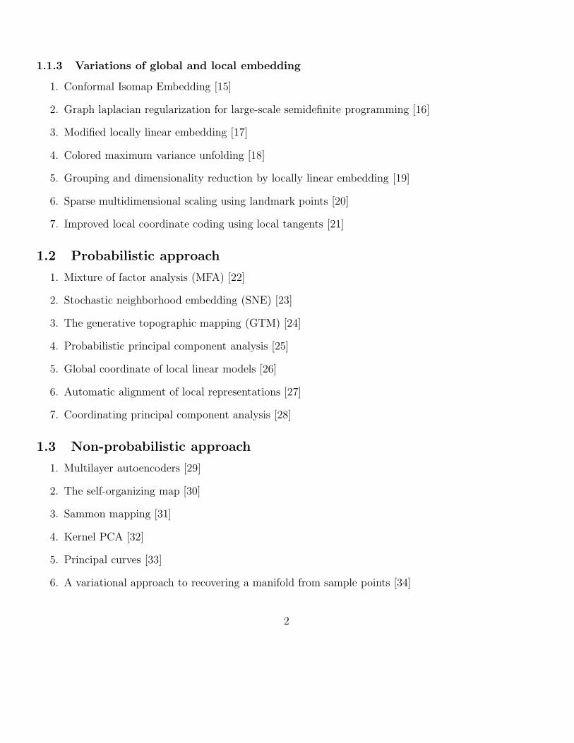
[61] E. Levina and P.J. Bickel, “Maximum likelihood estimation of intrinsic dimension,” Ann Arbor MI,vol. 48109, pp. 1092, 2004.
[62] J.A. Costa and A.O. Hero III, “Manifold learning using euclidean k-nearest neighbor graphs [imageprocessing examples],” in Acoustics, Speech, and Signal Processing, 2004. Proceedings.(ICASSP’04).IEEE International Conference on. IEEE, 2004, vol. 3, pp. iii–988.
[63] K.W. Pettis, T.A. Bailey, A.K. Jain, and R.C. Dubes, “An intrinsic dimensionality estimator fromnear-neighbor information,” Pattern Analysis and Machine Intelligence, IEEE Transactions on, ,no. 1, pp. 25–37, 1979.
[64] M. Fan, H. Qiao, and B. Zhang, “Intrinsic dimension estimation of manifolds by incising balls,”Pattern Recognition, vol. 42, no. 5, pp. 780–787, 2009.
[65] C. Bouveyron, G. Celeux, S. Girard, et al., “Intrinsic dimension estimation by maximum likelihoodin probabilistic pca,” in 73rd Annual Meeting of the Institute of Mathematical Statistics, Gothenburg,Sweden, 2010.