M/M/C/K/N systems: part II - TUT analysis and dimensioning I D.Moltchanov, TUT, 2013 2. M/M/m...

M/M/C/K/N systems: part II

Lecturer: Dmitri A. Moltchanov

E-mail: [email protected]

http://www.cs.tut.fi/kurssit/ELT-53606/

Network analysis and dimensioning I D.Moltchanov, TUT, 2013

OUTLINE:

• M/M/1 queuing system with state-dependent arrivals;

• M/M/m queuing system;

• M/M/m/m queuing system;

• M/M/1/K queuing system;

• M/M/1/∞/K queuing system;

• M/M/∞/-/K queuing system.

• Service time variation in M/-/C/K/N systems.

Lecture: M/M/C/K/N systems: part II 2


1. M/M/1 with state dependent arrivalsWhat we assume here:

• rate of the arrival is slowing down when the state goes up;

• where it may occur: some feedback mechanism controlling arrivals.

Parameters are given as follows:

λk =λ

k + 1, k = 0, 1, . . . ,

µk = µ, k = 1, 2, . . . ,

µ0 = 0. (1)

0 1 2 i... ...

2ll

3l

il

1il

+

m m m m m

Figure 1: Birth-death process of M/M/1 queuing system with state dependent arrivals.



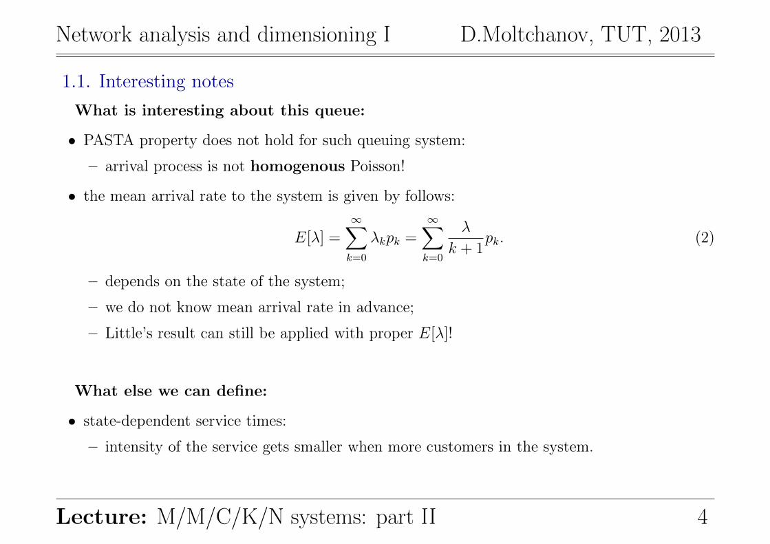
1.1. Interesting notes

What is interesting about this queue:

• PASTA property does not hold for such queuing system:

– arrival process is not homogenous Poisson!

• the mean arrival rate to the system is given by follows:

E[λ] =∞∑k=0

λkpk =∞∑k=0

λ

k + 1pk. (2)

– depends on the state of the system;

– we do not know mean arrival rate in advance;

– Little’s result can still be applied with proper E[λ]!

What else we can define:

• state-dependent service times:

– intensity of the service gets smaller when more customers in the system.



1.2. Steady-state distribution

Existence of steady-state distribution (capacity is infinite!):

• E[λ]/µ is always limited irrespective of initial λ

E[λ]

µ<∞. (3)

– even when λ >>> µ!

Solution for steady-state probabilities:

pk = p0

k−1∏i=0

λiµi+1

= p0

k−1∏i=0

λ

(i+ 1)

1

µ= p0

(λ

µ

)k1

k!, k = 1, 2, . . . , (4)

• where we can find p0 from normalizing condition:

p0 = 1−∞∑i=1

pk = 1−∞∑i=1

p0

(λ

µ

)k1

k!= e−(λ/µ). (5)

• λ is the arrival rate that decreases as the state number increases.



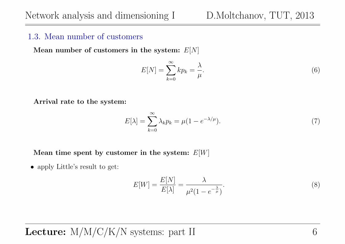
1.3. Mean number of customers

Mean number of customers in the system: E[N ]

E[N ] =∞∑k=0

kpk =λ

µ. (6)

Arrival rate to the system:

E[λ] =∞∑k=0

λkpk = µ(1− e−λ/µ). (7)

Mean time spent by customer in the system: E[W ]

• apply Little’s result to get:

E[W ] =E[N ]

E[λ]=

λ

µ2(1− e−λµ ). (8)



2. M/M/m queuing systemNote the following:

• the system has m servers each of which requires 1/µ time to serve customer;

• the birth-death process has the following parameters:

λk = λ, k = 0, 1, . . . ,

µk = kµ, k = 1, 2, . . . ,m,

µk = mµ, k = m+ 1, . . . . (9)

Note: steady-state distribution exists when ρ = λ/(mµ) < 1.

0 1 m-1 m...

1ì 2ì 1)ì-(m mì 1)ì+(m

ë

...

ë ë ë ë

n-1 n ...

ë ë ë

mì mì mì

Figure 2: Birth-death process associated with M/M/m queuing system.




The equilibrium state distribution is given by product form solution:

pk = p0ρk

k!, k = 1, 2, . . . ,m,

pk = p0ρk

m!mk−m , k = m+ 1, . . . , (10)

• where p0 can be derived from normalizing condition:

p0 =

(m−1∑k=0

ρk

k!+

mρm

m!(m− ρ)

)−1. (11)

Note the following:

• M/M/m queues was (is) extensively used in teletraffic theory;

• example: waiting time to get the free line.



2.2. Performance measures

The most important measure:

• probability that arriving customer will wait which is given by:

C(m, ρ) =∞∑k=m

pk =

mρm

m!(m−ρ)∑m−1k=0

ρk

k!+ mρm

m!(m−ρ)

. (12)

– this formula is extensively tabulated in literature.

Mean number of customers in the buffer: E[NQ]

• we obtain it directly from steady-state distribution:

E[NQ] =∞∑k=m

kpk =pm

1− ρ

∞∑k=0

k(1− ρ)ρn = C(m, ρ)ρ

1− ρ. (13)

Mean waiting time in the buffer: E[WQ]

• using Little’s result we get:

E[WQ] =E[NQ]

λ= C(m, ρ)

ρ

(1− ρ)λ. (14)



3. M/M/m/m queuing systemNote the following:

• there are no waiting positions in this queue;

• capacity of the system is limited and equal to the number of servers.

Parameters of birth-death process are as follows:

λk = λ, k = 0, 1, . . . ,m− 1

λk = 0, k ≥ m− 1

µk = kµ, k = 1, 2, . . . ,m,

µk = 0, k > m. (15)

0 1 m-1 m...

1ì 2ì 1)ì-(m mì

ë ë ë ë

Figure 3: Birth-death process associated with M/M/m/m queuing system.




Note the following:

• customers enters the queue if at least one position is free!

• otherwise, the customer is immediately rejected: loss system!

Condition of existence of steady-state distribution:

• state-space is limited;

• system is always stable irrespective of λ/mµ!

Defining ρ = λ/µ, the steady-state distribution is given by:

pk = p0ρk

k!, k = 1, 2, . . . ,m,

pk = 0, k = m+ 1, . . . , (16)

• where from the normalizing conditions we get p0:

p0 =

(m∑k=0

ρk

k!

)−1. (17)




Application of the M/M/m/m queue:

• call service process between telephone exchanges.

Exchange

...

cu

sto

me

rs

Exchange...

m links

Figure 4: Using M/M/m/m as a model in telephone network.

Most important parameter: probability of blocking:

• probability that an arrival finds all server busy forcing customer to leave without service.

Note: blocking is often used to describe the situation when the system is full:

• we say this system is with blocking;

• we say customer is blocked, etc.



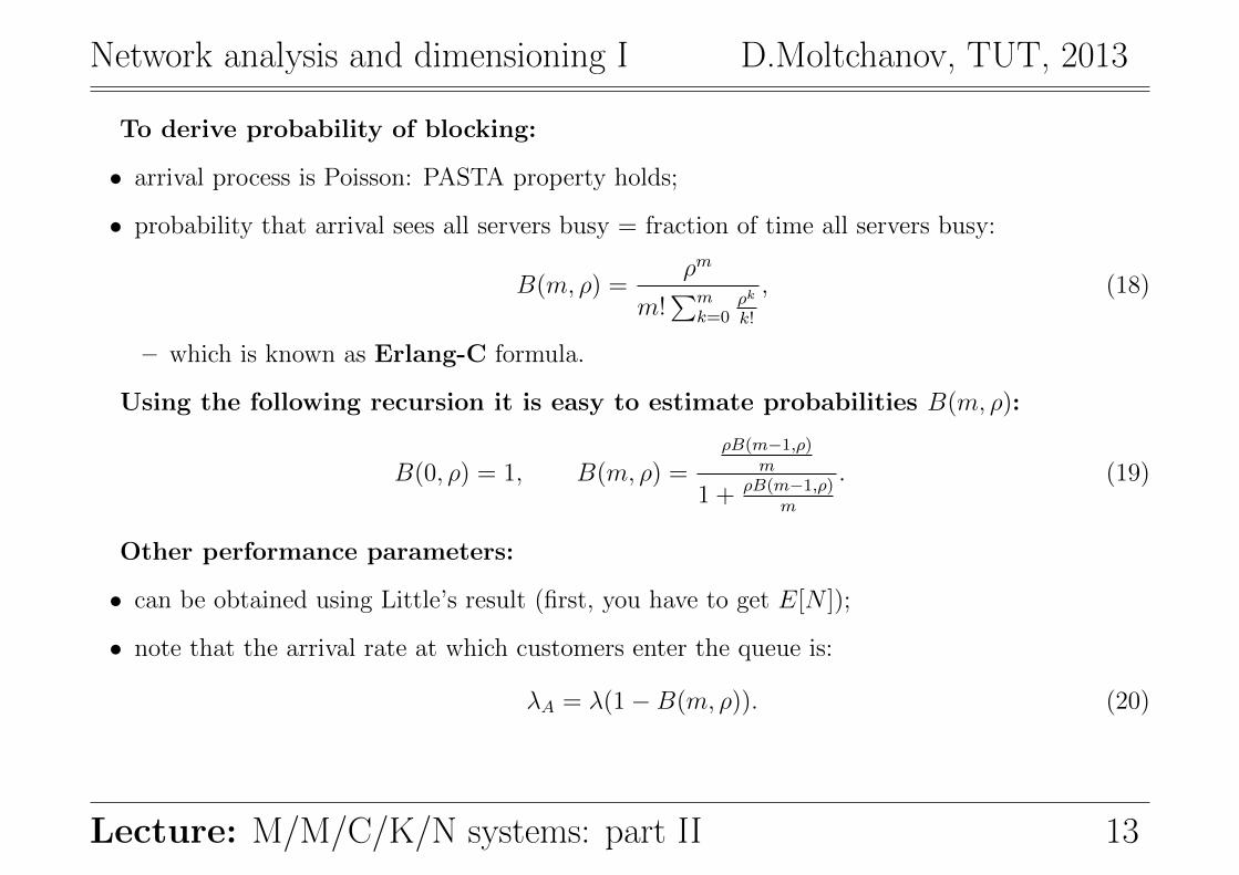
To derive probability of blocking:

• arrival process is Poisson: PASTA property holds;

• probability that arrival sees all servers busy = fraction of time all servers busy:

B(m, ρ) =ρm

m!∑m

k=0ρk

k!

, (18)

– which is known as Erlang-C formula.

Using the following recursion it is easy to estimate probabilities B(m, ρ):

B(0, ρ) = 1, B(m, ρ) =ρB(m−1,ρ)

m

1 + ρB(m−1,ρ)m

. (19)

Other performance parameters:

• can be obtained using Little’s result (first, you have to get E[N ]);

• note that the arrival rate at which customers enter the queue is:

λA = λ(1−B(m, ρ)). (20)



4. M/M/1/K queuing systemNote the following:

• frequently used in performance evaluation of packet networks;

• birth-death process associated with M/M/1/K has the following parameters:

λk = λ, k = 0, 1, . . . , K − 1

λk = 0, k ≥ K

µk = µ, k = 1, 2, . . . , K,

µk = 0, k > k. (21)

0 1 K-1 K...

ì ì ì ì

Kë

1-Kë

2ë

1ë

Figure 5: Birth-death process associated with M/M/1/K queuing system.




Existence of steady-state distribution:

• state space of the system is limited: {0, 1, .., K};

• steady-state distribution exist for all λ and µ irrespective of λ/µ!

Steady-state distribution is given by:

pk = p0ρk, k = 1, 2, . . . , K, (22)

pk = 0, k = K + 1, . . . , (23)

• where p0 can be found from the normalizing condition:

p0 =(1− ρ)

(1− ρK+1)(24)

Note: from equilibrium state distribution all mean parameters can be found.



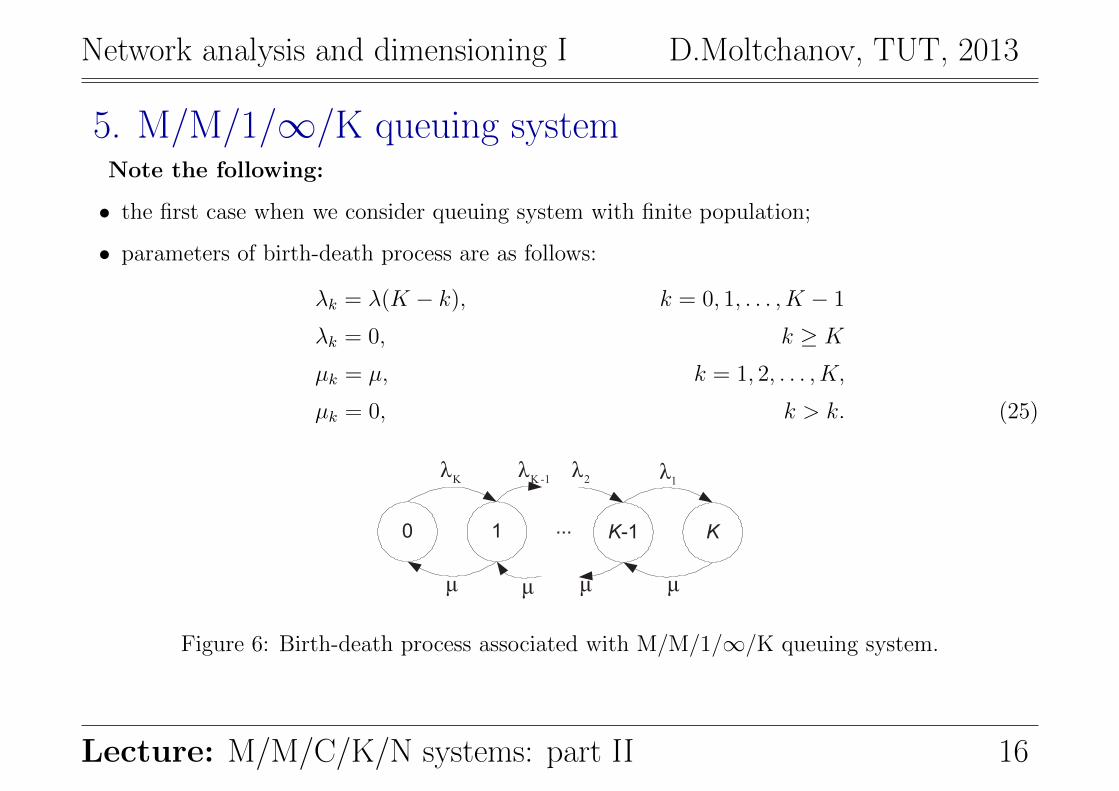
5. M/M/1/∞/K queuing systemNote the following:

• the first case when we consider queuing system with finite population;

• parameters of birth-death process are as follows:

λk = λ(K − k), k = 0, 1, . . . , K − 1

λk = 0, k ≥ K

µk = µ, k = 1, 2, . . . , K,

µk = 0, k > k. (25)

0 1 K-1 K...

ì ì ì ì

Kë

1-Kë

2ë

1ë

Figure 6: Birth-death process associated with M/M/1/∞/K queuing system.






• arrival rate decreases when state increases;


Defining ρ = λ/µ the steady-state distribution is:

pk = p0ρk K!

(K − k)!, k = 1, 2, . . . , K,

pk = 0, k > K, (26)

• where p0 can be found from normalizing condition:

p0 =

(K∑k=0

ρkK!

(K − k)!

)−1(27)

Note: performance parameters can be found immediately.



6. M/M/∞/-/KNote the following: number of servers need not be more K:

• limited population of customers.

Parameters of birth-death process are given:

λk = λ(K − k), k = 0, 1, . . . , K − 1

λk = 0, k ≥ K

µk = kµ, k = 1, 2, . . . , K,

µk = 0, k > k. (28)

0 1 K-1 K...

1ì 2ì 1)ì-(K Kì

Kë

1-Kë

2ë

1ë

Figure 7: Birth-death process associated with M/M/∞/-/K queuing system.







Defining ρ = λ/µ, steady-state distribution is given by:

pk = p0ρk K!

k!(K − k)!, k = 1, 2, . . . , K,

pk = 0, k > K, (29)

• where p0 can be found from normalizing condition:

p0 =

(K∑k=0

ρkK!

k!(K − k)!

)−1(30)

The mean arrival rate to the system is:

E[λ] =K∑k=0

λkpk = Kλ1

1 + ρ(31)




Mean number of customers in the system: E[N ]

E[N ] =Kρ

1 + ρ. (32)

Mean number of customers in the buffer: E[NQ]

E[NQ] = 0. (33)

• since the number of servers is infinite.

Mean time spent by customer in the system: E[W ]

E[W ] =E[N ]

E[λ]=

1

µ. (34)

• since any arriving customer immediately enters the server.

Mean time spent by customer in the buffer – E[Wb]

E[Wb] = 0. (35)

• since the number of servers is infinite.



7. Service time variation in M/-/C/K/N systemWhy service time variations:

• exponential distribution gives poor approximation;

• which other distribution we can use:

– Erlang distribution;

– hyperexponential distribution;

– Cox distribution;

– phase type distribution.

How we can analyze these systems:

• analyzing M/G/- queuing system;

– complete lack of memoryless property in service process.

• analyzing M/PH/- queuing systems and its special cases:

– we may still benefit from memoryless property of components.



7.1. Method of stages for M/Er/1

When this method is useful:

• service time is not exponentially distributed;

• service time is a combination of exponentials.

Consider the example of queuing system:

• Kendall’s notation: M/Er/1;

• Poisson arrivals, single server, infinite waiting room, Erlang service times.

Server: Erlang

Buffer

l 1m

Figure 8: Illustration of the queue of M/Er/1 type.



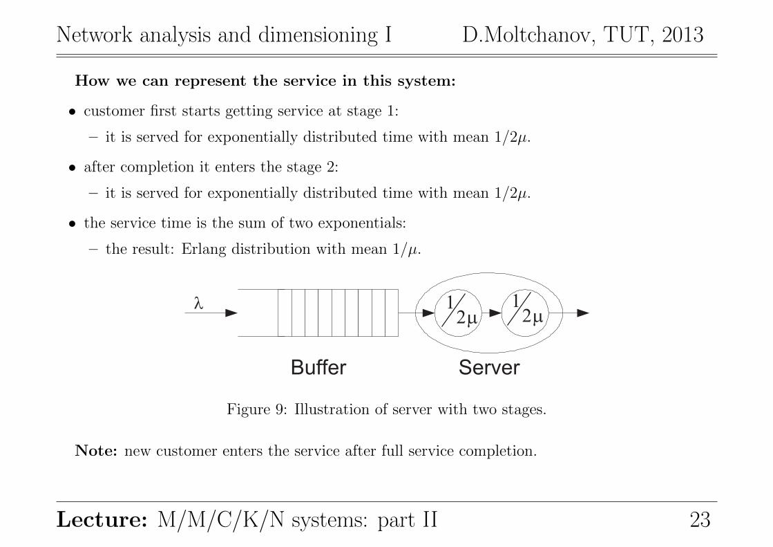
How we can represent the service in this system:

• customer first starts getting service at stage 1:

– it is served for exponentially distributed time with mean 1/2µ.

• after completion it enters the stage 2:

– it is served for exponentially distributed time with mean 1/2µ.

• the service time is the sum of two exponentials:

– the result: Erlang distribution with mean 1/µ.

ServerBuffer

l 12m

12m

Figure 9: Illustration of server with two stages.

Note: new customer enters the service after full service completion.



7.2. State of the system

State of the system:

• pair (n, j):

– n: total number of customers in the system;

– j: stage at which the current customer is served.

Do the following:

• SS = {0, 1, . . . }: number of customers in the system;

• SB = {1, 2}: phase of the service process;

• state space of the system is given by Cartesian product:

SS × SB = {0, 1, . . . } × {1, 2}, (36)



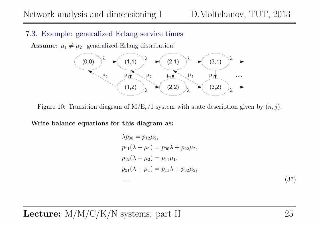
7.3. Example: generalized Erlang service times

Assume: µ1 6= µ2: generalized Erlang distribution!

(0,0) (1,1)

(1,2)

(2,1)

(2,2) (3,2)

(3,1)l l l l

lll

1m

1m 1

m2

m2

m2

m ...

Figure 10: Transition diagram of M/Er/1 system with state description given by (n, j).

Write balance equations for this diagram as:

λp00 = p12µ2,

p11(λ+ µ1) = p00λ+ p22µ2,

p12(λ+ µ2) = p11µ1,

p21(λ+ µ1) = p11λ+ p32µ2,

. . . (37)



Rewrite it as follows:

p12 =λ

µ2

p00,

p11 =λ(λ+ µ2)

µ1µ2

p00,

. . . (38)

Analyze as follows:

• express all pii, i = 1, 2, . . . as a function of p00;

• use normalizing condition to find p00.

This approach can be extended to:

• r stages of service time;

• finite number of waiting positions in the buffer;

• more general service time: hyperexponential, Cox, phase-type.



7.4. Alternative state description

What is bad about (n, j) description:

• (n, j) description is two-dimensional;

• when n or j are large it is getting complicated!

Another state description:

• number of uncompleted phases of work in the system:

– each waiting customer adds r phases of work;

– served customer adds j ≤ r phases of work:

• there is one-to-one correspondence between (n, j) and uncompleted phases of work:

(n, j) = (n− 1)r + j, (39)

– j is the number of phases left for customer currently being served;

– r is the total number of phases in service time;

– n is the number of customers in the system.



7.5. Example: Erlang service times

Assume: µ1 = µ2 = µ: Erlang distribution.

0 1 r r+1...

ì ì ì ì

ë

...

ë

Figure 11: Transition diagram of M/Er/1 system with a single state descriptor.

Note: any arrival adds r phases of work to the system.

Denote: pn be the steady-state probability that n phases of work are in the system:

• use global balance principle to get:

p0λ = p1µ,

pn(λ+ µ) = pn+1µ, n = 1, 2, . . . , r − 1,

pn(λ+ µ) = pn−rλ+ pn+1µ, n = r, r + 1, r + 2, . . . . (40)



Do not forget normalizing condition:

∞∑n=0

pn = 1, (41)

How to get the solution:

• one can solve equations to get uncompleted phases of work;

• we do not directly get any interesting quantity;

• after obtaining steady-state distribution we have to find distribution of states.


Date post:	14-Mar-2019
Category:	Documents
Upload:	leliem
View:	218 times
Download:	1 times

M/M/C/K/N systems: part II - TUT analysis and dimensioning I D.Moltchanov, TUT, 2013 2. M/M/m...

Documents