MNB Working Papers 2006/6. · Cochrane, Darrell Duffie, Zsuzsi Elek, Antoine Faure-Grimaud, Miklós...

MNB WORKING

PAPERS

2006/6

PÉTER KONDOR

Risk in Dynamic Arbitrage:

Price Effects of Convergence Trading

Risk in Dynamic Arbitrage:

Price Effects of Convergence Trading

May 2006

The MNB Working Paper series includes studies that are aimed to be of interest to the academic community, as well as

researchers in central banks and elsewhere. Starting from 9/2005, articles undergo a refereeing process, and their

publication is supervised by an editorial board.

The purpose of publishing the Working Paper series is to stimulate comments and suggestions to the work prepared

within the Magyar Nemzeti Bank. Citations should refer to a Magyar Nemzeti Bank Working Paper. The views

expressed are those of the authors and do not necessarily reflect the official view of the Bank.

MNB Working Papers 2006/6

Risk in Dynamic Arbitrage: Price Effects of Convergence Trading*

(A dinamikus arbitrázs kockázata)

Written by: Péter Kondor

Magyar Nemzeti Bank

Szabadság tér 8–9, H–1850 Budapest

http://www.mnb.hu

ISSN 1585 5600 (online)

* Email address: [email protected]. This paper is part of my PhD thesis. I am grateful for the guidance of Hyun Shin

and Dimitri Vayanos and the helpful comments from Péter Benczúr, Margaret Bray, Markus Brunnermeier, John

Cochrane, Darrell Duffie, Zsuzsi Elek, Antoine Faure-Grimaud, Miklós Koren, John Moore, Andrei Shleifer, Jakub

Steiner, Gergely Ujhelyi, Wei Xiong and seminar participants at Berkeley, Central Bank of Hungary (MNB), CEU,

Chicago, Columbia, Harvard, HEC, INSEAD, LBS, LSE, MIT, NYU, Princeton, Stanford, UCL, Wharton and the 2005

European Winter Meeting of the Econometric Society in Istanbul. All remaining errors are my own. I gratefully acknowl-

edge the EU grant ”Archimedes Prize” (HPAW-CT-2002-80054), the GAM Award and the financial support from the

MNB.

http://www.mnb.hu

Abstract 4

1. Introduction 5

2. A simple model of risky arbitrage 8

2.1. Assets 8

2.2. Local traders and the window of arbitrage opportunity 8

2.3. Arbitrageurs 11

3. The robust equilibrium 13

3.1. Equilibria in general 13

3.2. Equilibrium selection 16

4. Comparative statics and discussion 20

4.1. A calibrated example 22

5. Robustness 25

5.1. Partially flexible capital supply: reaching for yield 25

6. Conclusion 27

References 28

Appendix 29

A.1. Microfoundation of local traders’ behavior 29

A.2. Proofs 32

MNB WORKING PAPERS · 2006/6 3

Contents

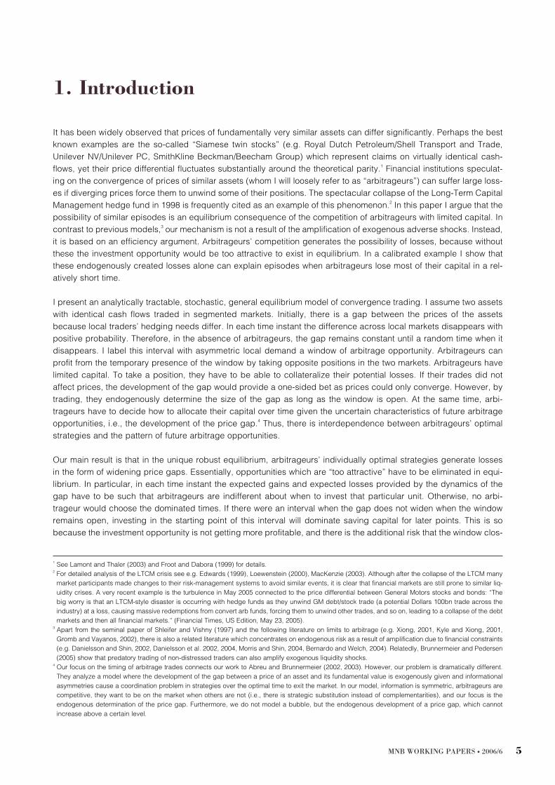
This paper studies the adverse price effects of convergence trading. I assume two assets with identical cash flows trad-

ed in segmented markets. Initially, there is gap between the prices of the assets, because local traders’ face asymmet-

ric temporary shocks. In the absence of arbitrageurs, the gap remains constant until a random time when the difference

across local markets disappears. While arbitrageurs’ activity reduces the price gap, it also generates potential losses:

the price gap widens with positive probability at each time instant. With the increase of arbitrage capital on the market,

the predictability of the dynamics of the gap decreases, and the arbitrage opportunity turns into a risky speculative bet.

In a calibrated example we show that the endogenously created losses alone can explain episodes when arbitrageurs

lose most of their capital in a relatively short time.

JEL classification: G10, G20, D5.

Keywords: Convergence trading, Limits to arbitrage, Liquidity crisis.

Abstract

A tanulmány az arbitrázs stratégiák árhatását vizsgálja. Tegyük fel, hogy létezik két nagyon hasonló értékpapír két szeg-

mentált piacon, amelyek árai idõlegesen eltérnek, mert a helyi piaci szereplõk keresletét eltérõ sokkok érik. Ha az arbi-

trázsõrök nincsenek jelen a piacon, az árak eltérése konstans egy véletlen idõpontig, amikor is a különbség megszûnik.

Megmutatom, hogy az arbitrázsõrök stratégiája csökkenti az árkülönbség nagyságát, de ugyanakkor megteremti a

veszteségek lehetoségét is: az árkülönbség pozitív valószínûséggel növekszik tetszõleges ideig. Minél több az arbi-

trázsõrök tõkéje a piacon, annál kevésbé elõre jelezhetõ az árkülönbség dinamikája. Az arbitrázslehetõség egy egyszerû

spekulatív befektetéssé válik. Egy kalibrált példában megmutatom, hogy az endogén módon keletkezett veszteségek

elegendõek olyan epizódok létrejöttéhez, amikor az arbitrázsõrök rövid idõ alatt tõkéjük nagy részét elvesztik.

Összefoglalás

4 MNB WORKING PAPERS · 2006/6


It has been widely observed that prices of fundamentally very similar assets can differ significantly. Perhaps the best

known examples are the so-called “Siamese twin stocks” (e.g. Royal Dutch Petroleum/Shell Transport and Trade,

Unilever NV/Unilever PC, SmithKline Beckman/Beecham Group) which represent claims on virtually identical cash-

flows, yet their price differential fluctuates substantially around the theoretical parity.

1

Financial institutions speculat-

ing on the convergence of prices of similar assets (whom I will loosely refer to as “arbitrageurs”) can suffer large loss-

es if diverging prices force them to unwind some of their positions. The spectacular collapse of the Long-Term Capital

Management hedge fund in 1998 is frequently cited as an example of this phenomenon.

2

In this paper I argue that the

possibility of similar episodes is an equilibrium consequence of the competition of arbitrageurs with limited capital. In

contrast to previous models,

3

our mechanism is not a result of the amplification of exogenous adverse shocks. Instead,

it is based on an efficiency argument. Arbitrageurs’ competition generates the possibility of losses, because without

these the investment opportunity would be too attractive to exist in equilibrium. In a calibrated example I show that

these endogenously created losses alone can explain episodes when arbitrageurs lose most of their capital in a rel-

atively short time.

I present an analytically tractable, stochastic, general equilibrium model of convergence trading. I assume two assets

with identical cash flows traded in segmented markets. Initially, there is a gap between the prices of the assets

because local traders’ hedging needs differ. In each time instant the difference across local markets disappears with

positive probability. Therefore, in the absence of arbitrageurs, the gap remains constant until a random time when it

disappears. I label this interval with asymmetric local demand a window of arbitrage opportunity. Arbitrageurs can

profit from the temporary presence of the window by taking opposite positions in the two markets. Arbitrageurs have

limited capital. To take a position, they have to be able to collateralize their potential losses. If their trades did not

affect prices, the development of the gap would provide a one-sided bet as prices could only converge. However, by

trading, they endogenously determine the size of the gap as long as the window is open. At the same time, arbi-

trageurs have to decide how to allocate their capital over time given the uncertain characteristics of future arbitrage

opportunities, i.e., the development of the price gap.

4

Thus, there is interdependence between arbitrageurs’ optimal

strategies and the pattern of future arbitrage opportunities.

Our main result is that in the unique robust equilibrium, arbitrageurs’ individually optimal strategies generate losses

in the form of widening price gaps. Essentially, opportunities which are “too attractive” have to be eliminated in equi-

librium. In particular, in each time instant the expected gains and expected losses provided by the dynamics of the

gap have to be such that arbitrageurs are indifferent about when to invest that particular unit. Otherwise, no arbi-

trageur would choose the dominated times. If there were an interval when the gap does not widen when the window

remains open, investing in the starting point of this interval will dominate saving capital for later points. This is so

because the investment opportunity is not getting more profitable, and there is the additional risk that the window clos-

1. Introduction

1

See Lamont and Thaler (2003) and Froot and Dabora (1999) for details.

2

For detailed analysis of the LTCM crisis see e.g. Edwards (1999), Loewenstein (2000), MacKenzie (2003). Although after the collapse of the LTCM many

market participants made changes to their risk-management systems to avoid similar events, it is clear that financial markets are still prone to similar liq-

uidity crises. A very recent example is the turbulence in May 2005 connected to the price differential between General Motors stocks and bonds: “The

big worry is that an LTCM-style disaster is occurring with hedge funds as they unwind GM debt/stock trade (a potential Dollars 100bn trade across the

industry) at a loss, causing massive redemptions from convert arb funds, forcing them to unwind other trades, and so on, leading to a collapse of the debt

markets and then all financial markets.” (Financial Times, US Edition, May 23, 2005).

3

Apart from the seminal paper of Shleifer and Vishny (1997) and the following literature on limits to arbitrage (e.g. Xiong, 2001, Kyle and Xiong, 2001,

Gromb and Vayanos, 2002), there is also a related literature which concentrates on endogenous risk as a result of amplification due to financial constraints

(e.g. Danielsson and Shin, 2002, Danielsson et al. 2002, 2004, Morris and Shin, 2004, Bernardo and Welch, 2004). Relatedly, Brunnermeier and Pedersen

(2005) show that predatory trading of non-distressed traders can also amplify exogenous liquidity shocks.

4

Our focus on the timing of arbitrage trades connects our work to Abreu and Brunnermeier (2002, 2003). However, our problem is dramatically different.

They analyze a model where the development of the gap between a price of an asset and its fundamental value is exogenously given and informational

asymmetries cause a coordination problem in strategies over the optimal time to exit the market. In our model, information is symmetric, arbitrageurs are

competitive, they want to be on the market when others are not (i.e., there is strategic substitution instead of complementarities), and our focus is the

endogenous determination of the price gap. Furthermore, we do not model a bubble, but the endogenous development of a price gap, which cannot

increase above a certain level.

es during the interval. But if arbitrageurs do not save capital for later time points, the gap will widen.

5

Hence, the com-

petition of arbitrageurs transforms the price process in a fundamental way. Without arbitrageurs the price gap could

only converge. While arbitrageurs’ activity reduces the price gap, it also generates potential losses: the price gap

widens with positive probability in each time instant.

The robust equilibrium is selected from a large number of possible equilibria by a simple selection method. This is the

only equilibrium which is compatible with the presence of arbitrarily small holding cost like a shorting fee. I show that

the inclusion of a positive shorting fee always results in a unique equilibrium with very similar properties to the robust

equilibrium. Indeed, as the holding cost diminishes the unique equilibrium of a world with positive holding cost con-

verges to the unique robust equilibrium of a world where trading is free. It is one of the non-robust equilibria, where

the gap is fully eliminated in all periods.

I demonstrate with the help of a calibrated example that these losses created by the competition of arbitrageurs can

be quantitatively substantial. In particular, these endogenous losses alone are enough to cause arbitrageurs to lose

most of their capital in a relatively short time with positive probability.

The robust equilibrium illustrates how arbitrageurs’ competition transforms the arbitrage opportunity. The change of

the gap is highly predictable when arbitrageurs are not present on the market: prices can only converge, just the time

of the convergence is uncertain. When arbitrageurs enter the market, divergence of price will be possible and the pre-

dictability of the change of the gap decreases. The more active arbitrage-capital enters the market, the more similar

the dynamics of the gap gets to a martingale process of unpredictable gap changes. Thus, arbitrageurs’ competition

transforms the arbitrage opportunity into a standard speculative bet where the probability weighted gains exceed the

probability weighted losses less and less. This implies that the presence of price differentials between very similar

assets does not imply the lack of arbitrage activity. In the robust equilibrium, the gap is never fully eliminated and

occasionally can be substantial. The valid question to valuate the activity of arbitrageurs is to what extent the dynam-

ics of the price gap is predictable.

The analytical tractability of our model stems from the reduced state space in our structure. The state of the window

influences the distribution of the price gap in a trivial manner. If the window closes in a given period, then the price

gap jumps to zero in that period and our modelled world ends. It is thus sufficient to characterize the path of the price

gap conditional on an open window. This result in a one-dimensional system, where one state variable, time (or equiv-

alently the aggregate level of capital at that point in time) determines the equilibrium development of the price gap

and the aggregate portfolio of arbitrageurs.

Our model naturally belongs to the literature on general equilibrium analysis of risky arbitrage (e.g., Gromb and

Vayanos, 2002, Zigrand, 2004, Xiong, 2001, Kyle and Xiong, 2001, Basak and Croitoru, 2000). However, to the best

of my knowledge, this paper is the first to show that competition of arbitrageurs alone can generate losses. In con-

trast to previous models focusing on potential losses in convergence trading (Shleifer and Vishny, 1997, Xiong, 2001,

Gromb and Vayanos, 2003, Liu and Longstaff, 2004), my mechanism is not based on the amplification of exogenous

shocks by the capital constraint. Instead, it is based on an efficiency argument. The reason for my unique finding is

that this is the first attempt to analyze the price effect of arbitrageurs whose dynamic portfolio choice is influenced by

uncertain future arbitrage possibilities over a long time span. Shleifer and Vishny (1997) and Gromb and Vayanos

(2002) touch upon one of the elements of our mechanism. Allowing uncertainty of future opportunities in one period

only, they show that arbitrageurs may be reluctant to take a maximal position as they fear that they will make losses

when the arbitrage possibility will be the most attractive. I show that allowing uncertainty over a longer time span, this

consideration is sufficient to transform the price process in a systematic way. In spirit, our paper is close to Liu and

Longstaff (2004) who argue that arbitrage with limited capital might lead to substantial losses. However, in their model,

this is a result of an exogenously defined price process, while my focus is on the determination of the price process.

The closest paper to my model in its stochastic structure is Xiong (2001) as he also considers arbitrage possibilities

MAGYAR NEMZETI BANK

MNB WORKING PAPERS · 2006/66

5

Interestingly, our argument is similar to the text-book mechanism of full elimination of price discrepancies by risk-neutral arbitrageurs with unlimited cap-

ital. There, price discrepancies providing positive expected profit would attract large investments and would be eliminated. In our case, price gaps which

cannot diverge would be similarly attractive possibilities and would be eliminated.

which are present for an uncertain time span. However, a crucial difference is that in his model, because of their spe-

cific preferences, the uncertainty over future arbitrage opportunities does not influence the decisions of arbitrageurs.

Furthermore, his results rely mostly on numerical results, while my equilibrium can be fully characterized analytically.

This paper proceeds as follows. In section 2, I present the structure of the model. In section 3, I derive the unique

robust equilibrium. In section 4, I discuss the results and in section 5, I analyze the robustness of my equilibrium.

Finally, I conclude.

INTRODUCTION


The structure of the model is based on three groups of agents: two groups of local traders in two segmented markets

and a group of arbitrageurs taking positions on both markets. A temporary asymmetry in the demand curves of local

traders creates an arbitrage opportunity. As the asymmetry is bound to disappear sooner or later, so is the arbitrage

opportunity. As arbitrageurs can take positions on both markets, they can exploit the price discrepancy. They are in the

focus of my analysis. They have limited capital so they have to decide how to allocate it over time given the distribution

of future arbitrage opportunities. Their strategies in turn determine the development of the price gap through market

clearing. Hence, there is interdependence between the distribution of future arbitrage opportunities and the individual

strategies of the arbitrageurs.

First, I describe the available assets in the economy, then I introduce traders and finally I present arbitrageurs.

2.1. ASSETS

There are two markets represented by two islands, i = A, B. On each island a single risky asset is traded. I will call them

A-asset and B-asset respectively. Both assets are in zero net supply. The two assets of the two islands have identical

payoff structure: both pays a R(td

) dividend regularly, at each time of dt = ∆d

,2∆d

..., where R(td

) is random, i.i.d., and

distributed according to the cumulative distribution function F (R) of bounded support with mean E (R) and ∆d

is an arbi-

trary positive constant. Time is infinite and except of the discreet timing of the dividend payments, the time of the model,

t, is continuous. A riskless bond with a zero net return is available on both islands as a storage technology.

2.2. LOCAL TRADERS AND THE WINDOW OF ARBITRAGE OPPORTUNITY

Each island is inhabited by a continuum of local traders: A-traders live on island A and B-traders live on island B. Each

local traders can trade only with the asset on her own island

6

and they are price takers. In the main text, I take local

traders’ demand curves as the primitives of the model. I provide possible microfoundations for the demand curve in

Appendix A.1.

The inverse demand curve of a representative local trader on island i in a given period t is

for i = A, B where θ i

(t) is the demand for the asset for the given price and p

~i

(h)h>t

is a stochastic function representing

the possible prices in all periods of the future. The arbitrage possibility arises because demand curves differ initially

across the two islands. Demand curves differ until a random time t

~

. In particular, for any t > t

~

i.e., for the same possible future prices A-traders are willing to hold the same amount of assets only for a higher price.

At period t

~

, the demand curves jump to the same level to

where p

~c

(h)h>t

is the stochastic function of future prices when demand curves coincide. I call the interval between time

0 and t

~

a window of arbitrage opportunity of random length. I also use the term that the window is open before time t

~

and closes at time t

~

. The distribution of t

~

is exponential: given that the window is still open, in each instant there is a con-

stant probability δ that the window closes. To endogenize price process when the window is closed, in Appendix I allow


2. A simple model of risky arbitrage

6

As my focus is not the source of the arbitrage possibility, I take market segmentation for local traders as given. Gromb and Vayanos (2002) and Zigrand

(2004) use similar assumptions. Nieuwerburgh and Veldkamp (2005) provide a mechanism which results in endogenous market segmentation.

for the possibility of reopening windows. However, in the main text we focus only on the first window, so for all practical

purposes, we can think of the random time t

~

as the end of the model-time and the price of the asset when the window

is closed, p

A

(t

~

) = p

B

(t

~

) = p

C

, as an exogenous constant. This treatment simplifies the exposition without changing the

results.

From the point of view of the analysis, the exact cause of the temporary difference in the demand curves is immaterial.

It can be an asymmetric shock to risk-aversion, to local traders’ income or any other type of demand shock.

7

The struc-

ture intends to catch the intuition that prices of similar assets which are traded by different groups of traders can tem-

porarily differ if arbitrageurs do not eliminate the price gap. The focus of this analysis is the activity of arbitrageurs in such

cases.

To be able to concentrate on arbitrageurs’ activity, it is necessary to keep the behavior of local traders as simple as pos-

sible. An important simplification is that the inverse demand of local traders does not have backward looking compo-

nents.

Assumption 1 The inverse demand curves d

i

(θ i

(t), p

~

(h)h>t

do not depend on past holdings of local traders or past prices,

θ i

(u) , p (u), for u < t; and i = A;B.

This assumption implies that the analysis abstracts away from the wealth effects of past gains or losses on local traders’

demand. In the microfoundation provided in Appendix A.1, these features are justified by new local traders entering in

each time instant with fixed trading horizon. However, the intuition of the main results would also go through with more

general demand functions.

Assumption 1 and the i.i.d. distribution of dividends are the reasons of the fact that the only source of uncertainty influenc-

ing prices will be the state of the window.

8

Hence, the conditional distribution of future prices p

~i

(h)h>t

given that t > t

~

is

characterized by p

c

and a deterministic function:

where p

~i

(h)h>t

is the price in island i in period h if the window is still open. Hence, we can write the inverse demand func-

tions as

(1)

Naturally, all realized prices depend on the equilibrium actions of different group of agents.

For a moment, let us assume that there are no arbitrageurs who trade between markets, so both markets have to clear

separately. I will refer to this case as autarchy. In autarchy, the aggregate supply of the risky asset which has to be held

on each island is zero unit. It is natural to suspect that the price process will remain constant if neither the quantity, nor

the state of the window changes, i.e. in autarchy θ i

(t) = 0 hence p

i

(t) ≡ p

i*

Hence, autarchy prices of p

A*

, p

B*

are given as

the solution of the following equations

(1)

(2)

A SIMPLE MODEL OF RISKY ARBITRAGE


7

In the appendix, an example is provided where initially local traders have different, non-tradable, stochastic endowments which implies different hedging

needs. This difference in the endowment disapears in period

8

This would not be true if arbitrageurs, who give the other side of the market, were allowed to use the same external randomization device to coordinate

their actions. As I discuss it at the presentation of the arbitrageurs, I rule this possibility out.

where the constant as the second argument of the demand functions denotes a constant function. The next assumption

states that autarchy prices are well defined. This is guaranteed in the example provided in Appendix A.1.

Assumption 2 There is a unique solution, p

A

*; p

B

* of equations (2)-(3) for p

c

and p

B

* < p

c

< p

A

*:

In the absence of arbitrageurs, the gap between the prices of the two assets is constant. In particular, g* ≡ p

A

* – p

B

*,

when the window is open and it is g* ≡ p

A

*– p

B

* when the gap is closed. Without loss of generality I will assume that

g

A

* > 0. Since in autarchy the gap is constant until the uncertain time when it closes, it would provide a safe an very prof-

itable bet for anyone who could trade on both markets.

The following assumptions ensure that the inverse demand curves are well behaving.

Assumption 3 For any future prices, p

c

, p

i

(h)h>t

where p

A

(h)h>t

, p

B

(h)h>t

∈ [p

B

*, p

A

*], there exists a positive, finite, mini-

mal θ–

= θ–

(p

A

(h)h>t

, p

B

(h)h>t

) such that

Assumption 4 Let us define θ–

max

as

Then the inverse demand functions, d

i

(θ i

(t), p

i

(h)h>t

, p

c

), i = A, B exist, continuous and di¤erentiable in t for any

θ A

(t) ∈ [0, – θ–

max

], θ B

(t) ∈ [0, – θ–

max

] and p

A

(h)h>t

, p

B

(h)h>t

∈ [p

B

*, p

A

*]

Assumption 5 Let us suppose that there is a θ +

which satisfies

where the constant as the second argument of the demand functions denote a constant function. Then p

A

+ – p

B+

> g*

implies θ +

< 0 and p

A+

– p

B+

< 0 implies + θ +

> 0: Furthermore, for every such θ +

there are sufficiently small open sets

around θ +

and p

i+

that the inverse demand function is continuous in these sets.

Assumption 6 Suppose that (p

i+

(h)h≥t

, p

c

, θ i+

(t)) and (p

i–

(h)h≥t

, p

c

, θ i–

(t)) are two combinations of prices and quantities

which satisfy the demand function for trader i. and θ A+

(t), θ A–

(t) ∈ [0, θ max

], θ B+

(t), θ B–

(t) ∈ [–θ max

, 0], and p

i+

(h)h>t

,

p

i–

(h)h>t

∈ p

B

*; p

A

*. If for all h > t which , the distribution of possible pay-offs p

~+i

(h) – p

+i

(t) + ~Rh

stochastically

dominates p

~+i

(h) – p

–i

(t) + R

~

h

in the first order sense; then θ +i

(t) > θ –i

(t).

Assumption 3 is an innocuous requirement that the price gap can be eliminated with sufficiently large, opposite positions

on the two markets. Assumption 4 defines a relevant domain where continuous inverse demand functions has to exist.

Assumption 5 is a week regularity requirement which has to hold outside of this relevant domain of the inverse demand

functions. It requires that as long as arbitrageurs keep selling the expensive A asset and buying the cheap B asset and

the price gap remains constant if the window survives, the gap cannot increase above g*. Similarly, as long as arbi-

trageurs do the opposite, the price of the B-asset cannot exceed the price of the A-asset. Although, I will use Assumption

6 in other ways in the proofs too, its main role that it directly implies that the inverse demand functions are downward

sloping in the relevant domain.

Lemma 1 For any θ A

(t) ∈ [θ–

max

, 0], θ B

(t) ∈ [0, –θ–

max

] and p

A

(h)h>t

, p

B

(h)h>t

∈ [p

B

*, p

A

*], .

In Appendix A.1 I show that Assumptions 1-6 are automatically satisfied under some standard assumptions about the

utility functions of local traders.

MAGYAR NEMZETI BANK


2.3. ARBITRAGEURS

Because of the asymmetric demand shocks on the two markets, if markets on the two islands clear separately, there will

be a price differential of g* between asset prices, although the assets have identical dividend structure. Arbitrageurs can

reduce this gap by taking positions on both markets. Arbitrageurs are the model-equivalent of global hedge funds with

the resources and the expertise to discover such price anomalies and to take positions in distant local markets.

Arbitrageurs live forever, they are risk neutral and operate in a competitive environment: they are small and they have a

unit mass. Arbitrageurs take positions x

i

(t) on island i = A, B. To keep our analysis simple I assume that arbitrageurs

face with symmetric local markets in the following sense.

Assumption 7 If p

A

(h) – p

c

= p

c

– p

B

(h) for all h > t then

The main reason to make this assumption is to ensure that arbitrageurs take exactly opposite positions on the two mar-

kets, i.e., x

A

(t) = –x

B

t) = x (t). If markets are symmetric, choosing an optimal strategy for one of the markets and do the

exact opposite on the other markets must be optimal. This property makes the model much more tractable without the

loss of any significant intuitive content.

9

We can interpret this property that arbitrageurs engage in market neutral arbi-

trage trades. I call the composite asset of one long unit of the B-asset and one short unit of the A-asset the gap asset.

I will show that in equilibrium x (t) is non-negative, i.e., arbitrageurs always buy the cheap asset and sell the more expen-

sive one. I will label such strategy as short selling x (t) unit of the gap.

Note that if arbitrageurs were not financially constrained, the strategy of short selling the gap would be riskless and would

lead to unbounded profit. However, because of the financial constraints specified below, sometimes arbitrageurs are

forced to liquidate before the prices of the assets converge, which can (and in equilibrium will) lead to losses. In effect,

their strategy is neutral only to the random payoff of the assets, R(td

), but not to the endogenous fluctuations of relative

prices caused by the random time of t

~

and arbitrageurs’ trades. Consequently, their arbitrage strategy is risky.

When the window is closed, demand curves in the two markets coincide, the arbitrage opportunity disappears and arbi-

trageurs stay inactive. This validates are treatment of the price p

c

as a constant. I focus on the dynamic strategies of arbi-

trageurs during the interval of the open window of arbitrage opportunity. From the assumptions on the demand of traders,

it is simple to construct the inverse demand function for the gap asset

which determines the gap g (t) ≡ p

A

(t) – p

B

(t) as a function of arbitrageurs’ aggregate position x

–

(t) and future prices

given that the window is still open. To keep the notation clear, I use g

~

(t) for the size of the gap as a stochastic function

while g (t) will denote the realized gap in the case that t < t

~

, i.e., the conditional distribution of g

~

(h)h>t

given that the win-

dow was open in time t is

Because of Assumption 7, prices on the two markets will be always symmetric: g (t) = 2 (p

A

(t) – p

c

). Thus, we can use

the simpler notation of

A SIMPLE MODEL OF RISKY ARBITRAGE


9

The example of the microfoundation provided in Appendix satisfies this property. Both Xiong (2001) and Gromb and Vayanos (2002) make assumptions

to ensure that arbitrageurs do not take asymmetric positions across local markets. It simplifies the analysis substantially, because it implies that arbi-

trageurs’ trades are neutral to the uncertainty of assets’ payoff, Rt

. Xiong (2001) makes a direct assumption, while Gromb and Vayanos (2002) assume

that traders have CARA utility and opposite endowment shocks very similarly to the structure in our example in Appendix A.1.

The assumptions on local demand curves also imply the most important properties of g (·). The inverse demand function

for the gap asset, f x

–

(t), p

A

(h)h>t

, p

B

(h)h>t

is exists and continuous if x

–

(t) [0, θ–

max

] and p

i

(h)h>t

∈ [p

B

*; p

A

*] and it is decreas-

ing in x

–

(t). If there is no arbitrage activity either at present or in the future, the gap is g*. Thus, in terms of g (·), the

autarchy price is given as g* = g (0, g*).

Arbitrageurs are financially constrained by the following institutional environment. Each arbitrageur starts her activity with

the same amount of capital

10

, ν (0) = ν–

0

where ν–

0

is the aggregate capital available in the economy. They do not get any

extra funds as long as the window is open.

11

They need funds for their activity because arbitrageurs are required to fully

collateralize their potential losses. For example, if their largest potential loss on an invested unit in the next time instant

is g

··

(t) to take a position of the size ,

an arbitrageur has to be able to present ν (t) cash, i.e., deposit ν (t) on a

margin account as the maximal possible loss on each unit is g

··

(t). This assumption can also be regarded as the formal-

ization of endogenous margin requirements or VaR constraints. Putting it another way, the assumption requires that the

marked-to-market value of arbitrageurs portfolios together with their capital always has to be non-negative. This con-

straint is clearly endogenous. When potential losses are large, arbitrageurs need to present more cash to be able to take

positions of a given size. This endogeneity will play an important role in the analysis.

We are looking for a rational expectation equilibrium of the problem. In this equilibrium, both local traders and arbi-

trageurs maximize their utility for given prices and both local markets clears. There are two sources of uncertainty in this

model.

12

Both risky assets pay the random dividend t

~

and the window disappears in the random time t

~

. However, the

structure of the model implies that we can reduce the stochastic problem into a deterministic one. First, Assumption

implies that the demand curves of local traders are independent of the realized dividend, R (td

). Similarly, Assumption 7

implies that R (td

) will not influence arbitrageurs’ pay-off, because it cancels out from the value of their portfolio. Hence,

the only relevant source of uncertainty is the state of the window. At the same time, it is clear what happens when the

window is closed. The gap disappears, arbitrageurs do not take any positions and local markets clear independently.

Consequently, to find the equilibrium we only have to find the conditional values of the equilibrium variables for each peri-

od t given that the window is still open at that time, t < t

~

. Thus, the problem of arbitrageurs reduces to the problem of

(4)

The maximand shows that the relative probability that the window closes in time instant t is δe

–δt

. If this happens, the arbi-

trageur gains g (t) x (t) profit on her current holdings and she gets her cumulated profit or loss, v (t). The first constraint

shows the dynamics of the capital level of the arbitraguer. In each period, the capital level of the previous period is

adjusted for the current gains or losses, x (t) g

··

(t). The last inequality is the collateralization. constraint. It shows that arbi-

trageurs are not allowed to take a position in any period which would make them bankrupt if the window survived that

given period and if their liabilities are marked to market.

The solution of problem (4) is a continuous and differentiable function {x(t)}∞t=0

of conditionally optimal portfolios for each

period t, given that the window is still open, t < t

~

. This strategy has to be optimal given the continuous and differentiable

conditional gap path {g (t)}∞t=0

. It is an equilibrium if the aggregate positions {x

–

(t)}∞t=0

support this conditional gap path,

(5)

i.e., both local markets clear. In the next section I present the equilibrium.

MAGYAR NEMZETI BANK


10

There is no significance of ν0

being the same across arbitrageurs. The analysis would be virtually the same if the initial capital was distributed in any other

way.

11

In section 5 I will relax this assumption.

12

I do not allow for an exogenous randomization device which could be used by arbitrageurs to coordinate their random actions. Hence, it is not possible

that all arbitrageurs decide to do simultaneously a certain action with a given probability and another action with some other probability. This would be

an additional source of uncertainty in the model.

In this section I present the unique robust equilibrium of the model. I proceed in two steps. In first part, I show that

generally the model has a continuum of equilibria. In the second part I show that only one of these equilibria is robust

to a simple and plausible perturbation of the model. Namely, if arbitrageurs have to pay an arbitrarily small shorting

fee for their portfolio holdings, all equilibria is eliminated but one. I discuss the implications of this robust equilibrium

in section 4.

3.1. EQUILIBRIA IN GENERAL

When arbitrageurs choose their strategy, they have to solve an intertemporal capital allocation problem. For each peri-

od, each of them has to decide how much of her capital to commit to the arbitrage at that period and how much of it to

save for later. The danger of saving capital for later is that the window might close today, and the arbitrageur might miss

out on the opportunity. The danger of committing the capital today is that if the window gets wider the arbitrageur will

have less capital for investing exactly when the possibility would be more profitable.

13

I argue that the aggregate investment plan {x

–

(t)}∞t=0

and the conditional gap path {g (t)}∞t=0

in all but one equilibria (includ-

ing the only robust equilibrium) are characterized by the following three intuitive conditions.

1) The gap path, {g (t)}∞t=0

has to be such that each arbitrageur has to be indifferent in which period to invest a dollar,

because investing in any period gives the same positive expected profit.

2) The level of aggregate positions, {x

–

(t)}∞t=0

has to be such that markets clear for the given gap path, i.e.,

f (x

–

(t), g p (h)h>t

) = g (t) for all t.

3) The sum of all possible aggregate losses exactly drains up the aggregate capital of arbitrageurs

(6)

i.e., the multiperiod budget constraint is binding.

These three conditions are sufficient to describe equilibria, because of the following logic. The first condition describes gap

paths where each arbitrageur is indifferent how to allocate her money between periods. Such indifference paths are possi-

ble, because arbitrageurs are risk-neutral. If investment in each period gives the same expected profit, they will be indiffer-

ent. With the help of the market clearing conditions, we can figure out the aggregate levels of investment which are consis-

tent with each g (t). If arbitrageurs have enough capital to follow this investment strategy in the aggregate, i.e., it does not

violate the aggregate budget constraint, the strategy will be feasible on the individual level as well. For example, each arbi-

trageur might follow the same strategy. In this case the aggregate variables coincide with the individual ones. Note also that

if all the three conditions are satisfied, the strategy must be optimal for the given prices. Increasing some investment level

is impossible because the budget constraint is binding. Cutting back positions in some periods to be able to increase posi-

tions in other periods is pointless as all periods give the same expected profit. Decreasing some positions to save some

money and not to commit it to any periods is suboptimal, because there is positive expected profit in each period.

Unless ν–

0

is very large

14

, this three conditions describe a continuum of conditional gap paths which are all increasing and

converge to a finite positive level less than or equal to g*. The conditional gap path typically has an S shape: convex for


13

The provided arguments build on the fact that the aggregate position x

–

t

is always non-negative i.e. arbitrageurs never speculate on the widening of the

gap. We will show in the formal proof why it is the case. The intuition relies on the point that x

–

t

< 0 would be consistent only with a bubble path of gt

. But

a bubble path is not consistent with the finite level of aggregate capital of arbitrageurs.

14

When ν–

0

is very large, there is no gap path, {g(t)}∞t=0

and corresponding average position path, {x

–

(t)}∞t=0

which would imply . It is so, because

the left hand side of the budget constraint is bounded from above. Arbitrageurs cannot lose more than g*θ–

max

for any gap path where θ–

max

is the maxi-

mal position which is needed to push down the gap to 0 defined in Assumption 4.

3. The robust equilibrium

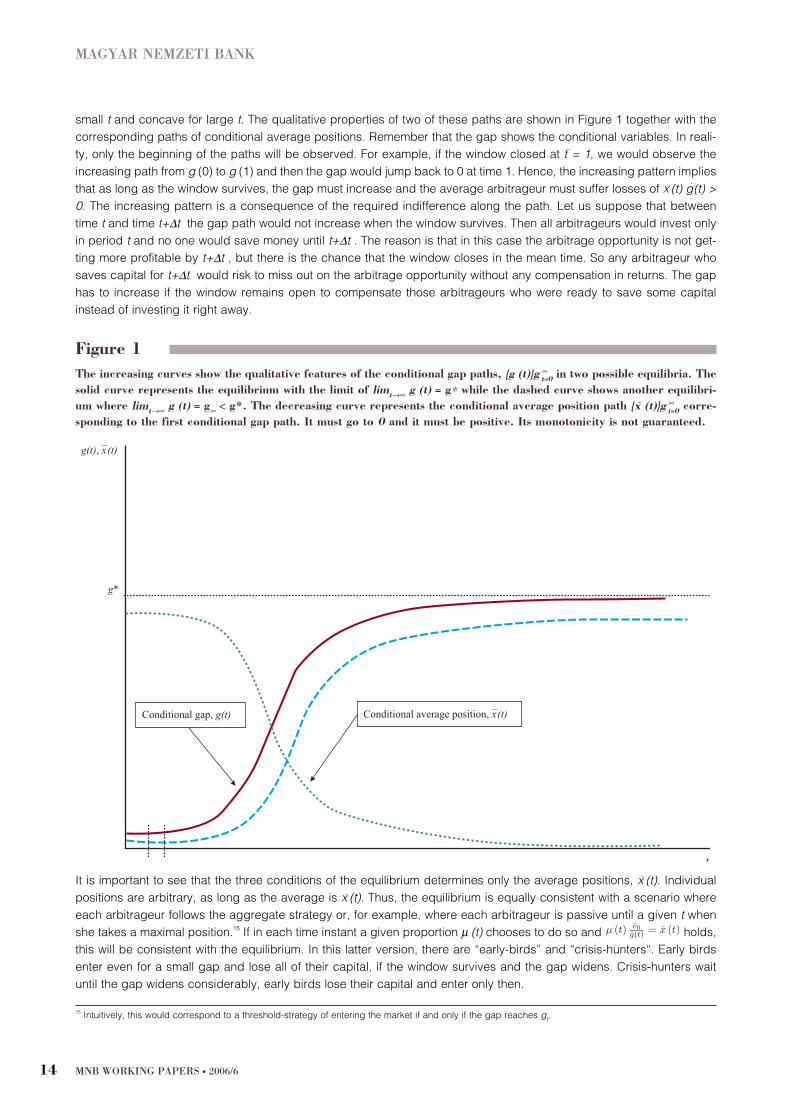
small t and concave for large t. The qualitative properties of two of these paths are shown in Figure 1 together with the

corresponding paths of conditional average positions. Remember that the gap shows the conditional variables. In reali-

ty, only the beginning of the paths will be observed. For example, if the window closed at t

~

= 1, we would observe the

increasing path from g (0) to g (1) and then the gap would jump back to 0 at time 1. Hence, the increasing pattern implies

that as long as the window survives, the gap must increase and the average arbitrageur must suffer losses of x

–

(t) g

··

(t) >

0. The increasing pattern is a consequence of the required indifference along the path. Let us suppose that between

time t and time t+∆t the gap path would not increase when the window survives. Then all arbitrageurs would invest only

in period t and no one would save money until t+∆t . The reason is that in this case the arbitrage opportunity is not get-

ting more profitable by t+∆t , but there is the chance that the window closes in the mean time. So any arbitrageur who

saves capital for t+∆t would risk to miss out on the arbitrage opportunity without any compensation in returns. The gap

has to increase if the window remains open to compensate those arbitrageurs who were ready to save some capital

instead of investing it right away.

It is important to see that the three conditions of the equilibrium determines only the average positions, x

–

(t). Individual

positions are arbitrary, as long as the average is x

–

(t). Thus, the equilibrium is equally consistent with a scenario where

each arbitrageur follows the aggregate strategy or, for example, where each arbitrageur is passive until a given t when

she takes a maximal position.

15

If in each time instant a given proportion µ (t) chooses to do so and holds,

this will be consistent with the equilibrium. In this latter version, there are “early-birds” and “crisis-hunters“. Early birds

enter even for a small gap and lose all of their capital, if the window survives and the gap widens. Crisis-hunters wait

until the gap widens considerably, early birds lose their capital and enter only then.

MAGYAR NEMZETI BANK


Figure 1

The increasing curves show the qualitative features of the conditional gap paths, {g (t)}g ∞t=0

in two possible equilibria. The

solid curve represents the equilibrium with the limit of limt→∞ g (t) = g∗ while the dashed curve shows another equilibri-

um where limt→∞ g (t) = g∞ < g*. The decreasing curve represents the conditional average position path {x

–

(t)}g ∞t=0

corre-

sponding to the first conditional gap path. It must go to 0 and it must be positive. Its monotonicity is not guaranteed.

Conditional average position, x—(t)

t

Conditional gap, g(t)

g(t), x—(t)

g*

15

Intuitively, this would correspond to a threshold-strategy of entering the market if and only if the gap reaches gt

.

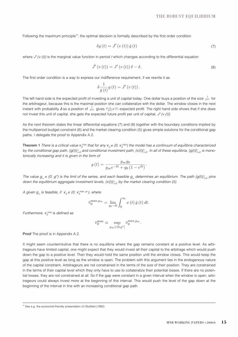
Following the maximum principle

16

, the optimal decision is formally described by the first order condition

(7)

where J′ (v (t)) is the marginal value function in period t which changes according to the differential equation

(8)

The first order condition is a way to express our indifference requirement, if we rewrite it as

The left hand side is the expected profit of investing a unit of capital today. One dollar buys a position of the size for

the arbitrageur, because this is the maximal position she can collateralize with the dollar. The window closes in the next

instant with probability δ so a position of gives expected profit. The right hand side shows that if she does

not invest this unit of capital, she gets the expected future profit per unit of capital, J′ (v (t)).

As the next theorem states the linear differential equations (7) and (8) together with the boundary conditions implied by

the multiperiod budget constraint (6) and the market clearing condition (5) gives simple solutions for the conditional gap

paths. I delegate the proof to Appendix A.2.

Theorem 1 There is a critical value ν–

0

max

that for any ν–

0

∈ (0, ν–

0

max

) the model has a continuum of equilibria characterized

by the conditional gap path, {g(t)}∞t=0

and conditional investment path, {x

–

(t)}∞t=0

. In all of these equilibria, {g(t)}∞t=0

is mono-

tonically increasing and it is given in the form of

The value g∞ ∈ (0, g*) is the limit of the series, and each feasible g∞ determines an equilibrium. The path {g(t)}∞t=0

pins

down the equilibrium aggregate investment levels, {x

–

(t)}∞t=0

by the market clearing condition (5).

A given g∞ is feasible, if ν–

0

∈ (0, ν–

0

max, g∞), where

Furthermore, ν–

0

max

is defined as

Proof The proof is in Appendix A.2.

It might seem counterintuitive that there is no equilibria where the gap remains constant at a positive level. As arbi-

trageurs have limited capital, one might expect that they would invest all their capital to the arbitrage which would push

down the gap to a positive level. Then they would hold the same position until the window closes. This would keep the

gap at this positive level as long as the window is open. The problem with this argument lies in the endogenous nature

of the capital constraint. Arbitrageurs are not constrained in the terms of the size of their position. They are constrained

in the terms of their capital level which they only have to use to collateralize their potential losses. If there are no poten-

tial losses, they are not constrained at all. So if the gap were constant in a given interval when the window is open, arbi-

trageurs could always invest more at the beginning of this interval. This would push the level of the gap down at the

beginning of the interval in line with an increasing conditional gap path.

THE ROBUST EQUILIBRIUM


16

See e.g. the economist-friendly presentation of Obstfeld (1992).

As the next Theorem states, there is one equilibrium which violates one of the three conditions described above. In this

equilibrium the conditional gap path is not increasing, but constant at the zero level, i.e., g (t) = 0 for all t. As this pro-

vide zero return on investment in any of the periods, arbitrageurs are indifferent between the periods. Just as before, the

aggregate positions are given by the market clearing condition, g (t) = f (x

–

(t), 0). However, the budget constraint will not

bind because the sum all potential losses in this equilibrium is 0. Arbitrageurs could increase their positions, but there is

no point to do so. The expected profit on any strategy is zero. The corresponding strategy profile will never violate the

collateralization. Constraint, because arbitrageurs are not limited if there are no potential losses.

Theorem 2 For any ν–

0

there is an equilibrium where g (t) = 0 for all t. This is the only additional equilibrium which is not

described by Theorem 1.

Proof. The proof is in Appendix A.2.

Intuitively, the multiplicity of equilibria can be seen as a coordination problem. The g (t) = 0 equilibrium is achievable,

but for this arbitrageurs should coordinate their future actions, i.e., they have to push down the gap in all states. As a

consequence, there will be no losses in any state of the world, arbitrageurs do not have to provide collateral for their

trades and the equilibrium is consistent with the budget constraint. Alternatively, if arbitrageurs coordinate on an equi-

librium with positive and increasing conditional gap path, the collateral constraint will be relevant because losses are

possible. In the following section, we will see that this coordination problem disappears by a small and plausible pertur-

bation of the model. Although the equilibrium where the gap is always fully eliminated seems intuitive, this – similarly to

all other equilibria but one – does not survive this equilibrium selection mechanism. This will leave us with the unique

robust equilibrium where the conditional gap path is increasing and it converges to g*.

3.2. EQUILIBRIUM SELECTION

I introduce a small perturbation to the model to select one of the many possible equilibria. Let us assume that there is a

small positive unit cost

16

, m of short selling the gap. If an arbitrageur takes a position of x (t) she has to pay a cost of

x (t) m. This is the carry cost of the position. The level of m is arbitrary as long as it is small in the following sense:

(9)

This perturbation changes Problem (4) only to the extent that the constraint for the development of the capital level is

modified to ν··

(t) = – (g

··

(t) + m) x (t).

We will see that this modified version have a unique equilibrium for any positive ν–

0

level. It will also turn out that as

m → ∞ the equilibrium converges to an equilibrium of the m = 0 case, the one where g∞ = g* and

Intuitively, the main reason why an arbitrarily small exogenous holding cost eliminates all but one equilibria lies in the

budget constraint. In any equilibria but the one where the conditional gap path converges to g* arbitrageurs commit to

invest at non-diminishing level for arbitrarily long. Even if the cost of investing is very small, sustaining such strategy for

a very long time has the potential to be extremely costly. Formally, the sum of all potential losses,

(10)

can converge only if limt →∞ x

–

(t) = 0. This implies that the conditional gap path must converge to g*.

17

It is also intuitive to follow the construction of the unique equilibrium when m>0. The qualitative features of this equilibri-

um is shown on Figure 2. The graph shows that if the window survives until time T, from time T on that period on arbi-

MAGYAR NEMZETI BANK


17

Assuming positive cost of holding is not the only way to eliminate all equilibria, but the robust equilibrium. For example, assuming positive cost of capi-

tal, i.e., that arbitrageurs pay back a fixed share of v0

to their investors in each period until they realize profit, would lead to very similar results.

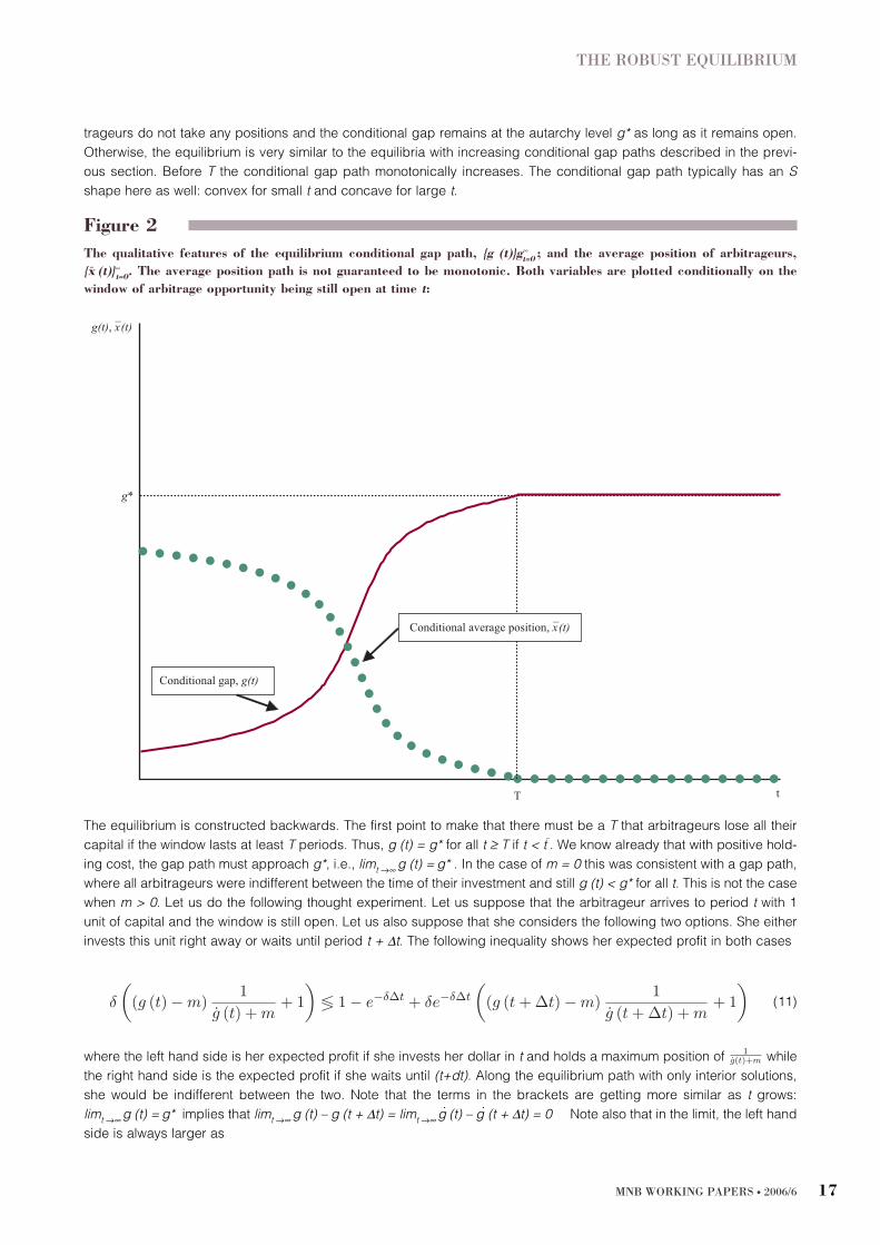
trageurs do not take any positions and the conditional gap remains at the autarchy level g* as long as it remains open.

Otherwise, the equilibrium is very similar to the equilibria with increasing conditional gap paths described in the previ-

ous section. Before T the conditional gap path monotonically increases. The conditional gap path typically has an S

shape here as well: convex for small t and concave for large t.

The equilibrium is constructed backwards. The first point to make that there must be a T that arbitrageurs lose all their

capital if the window lasts at least T periods. Thus, g (t) = g* for all t ≥ T if t < t

~

. We know already that with positive hold-

ing cost, the gap path must approach g*, i.e., limt →∞ g (t) = g* . In the case of m = 0 this was consistent with a gap path,

where all arbitrageurs were indifferent between the time of their investment and still g (t) < g* for all t. This is not the case

when m > 0. Let us do the following thought experiment. Let us suppose that the arbitrageur arrives to period t with 1

unit of capital and the window is still open. Let us also suppose that she considers the following two options. She either

invests this unit right away or waits until period t + ∆t. The following inequality shows her expected profit in both cases

(11)

where the left hand side is her expected profit if she invests her dollar in t and holds a maximum position of while

the right hand side is the expected profit if she waits until (t+dt). Along the equilibrium path with only interior solutions,

she would be indifferent between the two. Note that the terms in the brackets are getting more similar as t grows:

limt →∞ g (t) = g* implies that lim

t →∞ g (t) – g (t + ∆t) = limt →∞ g

⋅(t) – g

⋅(t + ∆t) = 0 Note also that in the limit, the left hand

side is always larger as



Figure 2

The qualitative features of the equilibrium conditional gap path, {g (t)}g∞t=0

; and the average position of arbitrageurs,

{x–

(t)}∞t=0

. The average position path is not guaranteed to be monotonic. Both variables are plotted conditionally on the

window of arbitrage opportunity being still open at time t:

Conditional gap, g(t)

g(t), x—(t)

g*

T t

Conditional average position, x—(t)

Intuitively, if the market tomorrow and today is very similar, there is no point to wait and risk to miss out on the opportu-

nity. Thus, there must be a large enough T, that at the instant before T the left hand side of (11) is strictly larger so arbi-

trageurs decide to invest all their capital and risk to lose all this capital if the window survives until T. Thus, x

–

= 0 and

g (t) = g* for all t ≥ T.

The observation that by T, arbitrageurs would be happy to invest all their remaining capital implies that the marginal value

function at T is given by this strategy is

Hence, with the help of the perturbed versions of (7) and (8)

and with the boundary condition g (T) = g*, we can construct the equilibrium conditional gap path backwards from time

T. This path will be monotonously increasing and makes each arbitrageur indifferent in which period to invest before T.

The last remaining question is where we should stop with this process: what is the value of T ? Time T is pinned down

by the budget constraint. In equilibrium, if the window survives, by period T arbitrageurs have to use up all their capital

to validate the definition of T, i.e.,

(12)

The proof of the next theorem ensures that this procedure indeed leads to a unique equilibrium.

Theorem 3 There is a unique equilibrium in the economy in terms of average positions, which consists of a period T a

path of average positions {x

–

(t)}∞t=0

and a conditional gap path {g (t)}∞t=0

. The equilibrium is characterized by the follow-

ing expressions:

(13)

and

(14)

Furthermore, {g (t)}

T

t=0

is strictly monotonically increasing in t.

MAGYAR NEMZETI BANK


Proof Details of the proof are in Appendix A.2.

After the construction of the equilibrium with m > 0 it might be unsurprising that as m diminish, T increases without bound

and the equilibrium converges to the equilibrium described in Theorem 1 with g∞ = g*. After all, the equilibrium with

m > 0 is also determined by the indifference condition, the market clearing condition and the budget constraint and we

also know that any arbitrarily small holding cost rules out any equilibria where limt→∞ ≠ g*. This is why I call the equilibri-

um where g∞ = g* the robust equilibrium of the system. This result is summarized in the next Proposition.

Theorem 4 If v

–

0

∈ (0,v

–

0

max,g*

), as m → 0, the equilibrium of the perturbed system with m > 0 converges to the equilibrium

described in Theorem 1 where

(16)

Proof The proof is in Appendix A.2.

In the next section I discuss the properties of the robust equilibrium.



The main observation of this model is that arbitrageurs’ individually optimal strategies transform the arbitrage opportuni-

ty in a systematic way. First of all, arbitrageurs create their own potential losses. Remember the assumption that if arbi-

trageurs were not present on the market, the gap between the prices could never increase. Hence, the first arbitrageur

who could bet (without affecting prices) on the convergence would make a sure profit without having the chance of suf-

fering a loss in any time point. However, as soon as a positive mess of arbitrageur enter the market, in each period when

the window remains open, the gap increases. The average arbitrageur loses some capital.

It is interesting to contrast the presence of endogenous losses with the intuition of other models of limits to arbitrage, e.g.,

Shleifer and Vishny (1997), Xiong (2001), Gromb and Vayanos (2002) and Liu and Longstaff (2004). They all emphasize

that arbitrageurs might lose money because they might be forced to liquidate early if the gap widens. However, in those

models the initial widening of the gap happens for reasons which are exogenous to the arbitrageurs’ strategies. In par-

ticular, it is a result of noise traders trading against fundamentals (Shleifer and Vishny, 1997, Xiong, 2001, Gromb and

Vayanos, 2002) or an exogenously specified price process (Liu and Longstaff, 2004). These models focus on different

mechanisms which amplify the first exogenous shock. In contrast, the mechanism of my model is not based on an ampli-

fication argument. If arbitrageurs do not trade, the price gap cannot widen in any way. The possibility of diverging prices

is the equilibrium consequence of arbitrageurs individually optimal actions..

The mechanism of this model is based on an efficiency argument. In this respect, it bears some resemblance to the stan-

dard text-book case for efficient markets. In the text-book equilibrium, different prices for assets with the same cash-flows

cannot exist, because they would provide a very attractive opportunity for arbitrageurs. Thus, arbitrageurs would instant-

ly make large bets on the convergence, which would automatically eliminate the anomaly by pushing the prices to the

same level. The robust equilibrium gap path of my model is sustained by a similar mechanism. Along the gap path, each

arbitrageur is indifferent when to invest. However, if in any time, the gap were above the equilibrium path, it would pro-

vide a very attractive opportunity for the arbitrageurs. All of them would prefer to save money until this time instant and

invest all if the window is still open. But this would push back the gap to the equilibrium level. Similarly, no one would

invest at times in which the gap is below the equilibrium path, which would increase the gap at that period up to the equi-

librium level. The main difference here compared to the text-book case is that the aggregate capital level of arbitrageurs

is limited, so the gap is not fully eliminated. In this sense, we can label the equilibrium price gap as “limited-arbitrage-

free prices”.

18

Probably, the most intuitive way to see how arbitrageurs action transforms the arbitrage opportunity is to have a look on

the effect on the predictability of the gap. As we expect from an arbitrage opportunity, in autarchy the expected change

of the gap is highly predictable from the current gap:

i.e., prices are expected to converge. In the robust equilibrium, from equation (16)

(17)

with


4. Comparative statics and discussion

18

Another potentially important difference here compared to the text-book case is that arbitrageurs have to compare current prices with expected future

prices to decide on their actions. In the text-book arbitrage trades they only have to realize a mismatch in contemporanous prices. Thus, possibly our

mechanism requires more sophisticated arbitrageurs. As real-world equivalents of arbitrageurs are hedge funds, institutions considered to be among the

most sophisticated investors, this should not be a problem.

where M

t,h

(v

–

0

) depends on v

–

0

through g0

. In following proposition, we will see that although the difference

(18)

is always positive, it is decreasing and goes to zero as the level of capital increases towards its maximum, v

–

0

max,g*

. Thus,

although the gap is always expected to decrease, as there are more and more arbitrageurs enter the market, the gap

approaches a martingale process. Arbitrageurs’ competition with limited capital turn arbitrage into standard speculative

bets where the probability-weighted gains are – almost – equal to the probability weighted losses.

Proposition 1 In the robust equilibrium

1) for any fixed t, and

2) as v

–

0→ v–

0

max,g*

, g (t) approaches a martingale

Proof It is clear from the proof of Theorem 1 that and limv

–

0

→v

–

0

max,g* g0

= 0. All statements of the proposition are

straightforward consequences of this fact and equations (16), (17) and

(19)

from the proof of Theorem 1.

The fact that more arbitrage-capital in the market pushes the arbitrage opportunity into the direction of a standard spec-

ulative asset also sheds some new light on pricing anomalies like “Siamese twin stocks”

19

. This model suggests that if

we believe that arbitrageurs have limited capital, we should not valuate positive gaps between very similar assets as

the lack of arbitrage activity. The gap is never fully eliminated by arbitrageurs. What we should check is to what extent

these price gaps move in a predictable way. If there is a strong mean reversion then it indeed suggests a week arbi-

trage activity. However, if the gap process moves in a rather unpredictable way, it might be a sign of active influence

of rational arbitrageurs.

Another way to look at the effect of arbitrageurs’ competition on prices is to analyze the expected profit of arbitrage. Note

that the value function at time 0, J (v0

) is the expected profit of an arbitrageur by definition,

where the last equation comes from expression (19). From Proposition 1, it is clear that more aggregate arbitrage-

capital decreases the available expected profit. This is quite intuitive if we think of the aggregate level of capital is the

measure of arbitrageurs who know about the arbitrage opportunity. If the arbitrage opportunity is widely known among

potential arbitrageurs then they all enter the market and the available profit is reduced by the competition. But if only

few arbitrageurs find a new opportunity, they can expect large expected profit. This is also consistent with the reduc-

tion of predictability when the arbitrage capital is high in the market. Less predictable prices provide less expected

profit.

Given its level of abstraction, it might be surprising that – under certain circumstances – this model can also generate

the skewed distribution of returns observed in the data. In particular, in the robust equilibrium the distribution of the aver-

COMPARATIVE STATICS AND DISCUSSION


19

See Lamont and Thaler (2003) and Froot and Dabora (1999) for details.

age arbitrageur’s total return is skewed toward the left

20

if the level of aggregate positions is decreasing, .

21

This

is so, because in this case, the realized return on capital of the average arbitrageur given that the window closes at t

~

,

is decreasing with the length of the window. Intuitively, the average arbitrageur loses capital as the window

gets longer, if her position decreases, because if she liquidates a part of her portfolio as the gap widens, she suffers

losses on the liquidated units. She makes a net gain if the window closes instantly as , but if the window is

long enough, she loses most of her capital. Since longer windows occur with smaller probability, the average arbitrageur

will make a positive net return with large probability and larger losses with smaller probability during each window. The

next lemma shows the formal result.

Proposition The density function of the average arbitrageur’s gross return in each opportunity is given by

for all t

~

>0

where is decreasing in t

~

if and . Thus, if this distribution is skewed

toward the left.

Proof The statement is the direct consequence of the exponential distribution of t

~

and

In the next section, I present a calibrated example to quantify the risk and level of endogenous losses in equilibrium.

4.1. A CALIBRATED EXAMPLE

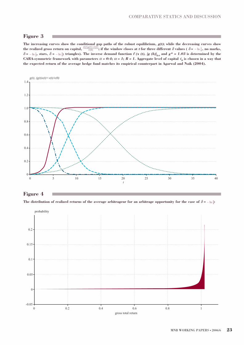
A simple calibration exercise is illustrated by Figure 3. The increasing curves show three conditional gap paths of the

robust equilibrium corresponding to three different δ values ( )

21

. The decreasing curves show the

total gross return of the average arbitrageur for different δ values given that the window closes in period t

~

,

I use the CARA-symmetric framework defined in Appendix A.1 for the specification of the inverse demand function

f (x

–

(t), g (h)h>t

). I choose parameters

22

which imply g* = 2. With these parameters Assumptions 1-3 are satisfied.

23

For

the calibration I assume that each unit interval corresponds to a week. Then I choose the aggregate level of capital, v

–

0

in each case in a way to ensure that the annualized return of an average arbitrageur following the optimal strategy cor-

responds to the historical average return of hedge funds between 1994-2000 (see Agarwal and Naik, 2004).

24

MAGYAR NEMZETI BANK


20

We analyze the arbitrageurs’ total return during a window of arbitrage opportunity, instead of their period per period return. On one hand it is reasonable

as the observed skewness of hedge funds’ returns in the empirical literature (e.g. Agarwal and Naik, 2004) comes from monthly or quaterly data, while in

our calibration excercise a period corresponds to a week and the expected length of a window ranges from 9 days to 1 month. On the other hand, the fact

that the length of a window is a random variable while returns in the empirical literature are calculated for a fixed interval makes the interpretation harder.

For results on the distribution of returns for a fixed interval, more structure would be needed on the distribution of arbitrage opportunities an arbitrageur

can find during a fixed interval. However, as long as the interval is long relative to the expected length of a window, our result is expected to hold.

21

These δ values imply that the window survives any unit interval with probability ¼, ½ and ¾ respectively.

22

In terms of the example in the appendix, I choose a level of absolute risk aversion of α = 0.5 the size of the endowment shock is ω = 1 and the variance

of the dividend rate is σ 2

= 1.

23

We show in Appendix A.1.1 how to determine g* from the primitives and how to ensure that Assumptions 1-3 are satisfied.

24

The annualized return is calculated by valuating the marginal value function at period 0 and by using the fact that expected length of the window is 1/δweeks by the properties of the exponential distribution. In each case the annualized net return is 17.23%. The Matlab 7.0 code of the calibration exercise

is available on request from the author.

COMPARATIVE STATICS AND DISCUSSION


Figure 3

The increasing curves show the conditional gap paths of the robust equilibrium, g(t); while the decreasing curves show

the realized gross return on capital, ; if the window closes at t for three different δ values ( δ = , no marks,

δ = , stars, δ = ; triangles). The inverse demand function f (x (t), {g (h)}h>t

and g* = 1.03 is determined by the

CARA-symmetric framework with parameters α = 0:4; ω = 1; R = 1. Aggregate level of capital v–

0is chosen in a way that

the expected return of the average hedge fund matches its empirical counterpart in Agarwal and Naik (2004).

1.4

1.2

1.0

0

0.2

0.4

0.6

0.8

0 5 10 15 20 25 30 35 40t

g(t), (g(t)x(t)+v(t)/v(0)

Figure 4

The distribution of realized returns of the average arbitrageur for an arbitrage opportunity for the case of δ = :

0.2

0.15

0.1

0.05

0

-0.050 0.2 0.4 0.6 0.8 1

gross total return

probability

The main lesson from the calibration exercise is that even in the limit equilibrium, price effects from the competition of

arbitrageurs alone can explain episodes when arbitrageurs lose most of their capital relatively fast. Consistently with

Theorem 1 and Lemma 2, Figure 3 illustrates that the longer the window the wider the gap and the larger the loss of the

average arbitrageur. In particular, the total gross return on capital exceeds one if the window closes early. Hence, arbi-

trageurs make a positive profit only in these large probability cases. If the window survives longer, the average arbi-

trageur loses a larger proportion of her capital. The following two tables quantify our observations.

The first table shows the minimum length of the window (rounded to the nearest half unit) which is necessary to wipe out

a given proportion of the initial capital of arbitrageurs, while the second table shows the corresponding probabilities of

these events. For example, the second cell of first row in the first table shows that if δ = – ln ½ and the window remains

open for at least 5 weeks, the average arbitrageur will make a negative net return. The same cell in the second table

shows that this happens with the probability of 2.2%. The second cell in the second row of the tables show that if the

window is still open after 2 and a half month, the average arbitrageur loses 50% of her initial capital and the probability

of this event is 1%. This may seem a small probability event, but it is important to note that this is the probability of such

crisis if arbitrageurs bet in a single window of arbitrage opportunity. When δ = – ln ½ the expected length of a window

is about 10 days. Most probably arbitrageurs would take positions in a large number of subsequent windows in each

year. Hence, the probability that one of these windows is long enough to generate a crisis with substantial losses can be

significant.

Finally, Figure illustrates the distribution of the total gross return of the average arbitrageur in a window of arbitrage

opportunity for the case of δ = – ln 0.75. The distributions for the other two cases are very similar. The Figure demon-

strates – consistently with Lemma 2 – that the average arbitrageur will make a small profit most of the time, while she will

make large losses infrequently.

MAGYAR NEMZETI BANK


weeks δ = – ln ¼ δ = – ln ½ δ = – ln ¾

0% 3 5 10

50% 5.5 9.5 19.5

90% 10 12.5 27

% δ = – ln ¼ δ = – ln ½ δ = – ln ¾

0% 0.7 2.2 4.8

50% 0.01 1 0.3

99% 10

–7

0.01 0.05

The main observation of this model is that arbitrageurs following their individually optimal strategies create losses

endogenously. Their competition does not eliminate the price gap fully, but reduces the predictability of relative price

movements: transforms the arbitrage opportunity into a speculative bet. I expect that this result is robust to a wide range

of set-ups, but I consider three of the assumptions particularly important for this result. The first one is that the duration

of the window of arbitrage opportunity is uncertain and, in particular, that it can be arbitrarily long. An example for the

departure from this assumption is Gromb and Vayanos (2002). They assume a window with a fixed length i.e. the gap

disappears in an exogenously fixed period. They show – in contrast with our result – that the gap path will typically

decrease in that case. The other critical assumption is that arbitrageurs take both prices and the probability of conver-

gence as given. Zigrand (2004) presents a model where there is imperfect competition among arbitrageurs, while Abreu

and Brunnermeier (2002,2003) analyze the case where arbitrageurs are strategic and the time of convergence is deter-

mined in equilibrium. The third important assumption is that there is no capital inflow into the market during the window

of arbitrage opportunity. In this section, I focus on the implications of relaxing this assumption.

I argue that the effect of more flexible capital supply in the industry depends on the exact way we think about it. One

view is that as the gap gets wider and the arbitrage opportunity gets more profitable, so we should expect more capital

to enter into the industry. I will focus on this argument in the next section and show that in certain scenarios the equilib-

rium remains virtually unchanged, even if there is a positive relationship between profitability and the level of the enter-

ing capital. Another argument is related to the agency view of the arbitrage sector. Hedge funds (arbitrageurs) get their

capital from investors who delegate their portfolio decisions hoping that hedge funds know and have access to better

opportunities. However, there investors do not have exact information on the abilities and opportunities of hedge funds.

Hence, investors use arbitrageurs’ past performance as a signal about their abilities. If this effect is strong, there might

even be a capital outflow from the market when the gap increases as this is the time when arbitrageurs lose money. Here

I do not consider this case, but in Kondor (2006) I adjust the current set up with a formal model of this agency problem

and analyze the additional effects on arbitrageurs strategies and equilibrium prices in detail.

5.1. PARTIALLY FLEXIBLE CAPITAL SUPPLY: REACHING FOR YIELD

Let us suppose that there is a positive relationship between the expected profit in the arbitrage market and the level of

capital inflow in a given period. The idea is that there is an external pool of investors who are faced with different costs

or outside options. In each period they decide whether to enter the arbitrage market for the given prices and future

opportunities. As the arbitrage market gets more profitable, more investors decide to join. This is consistent with the

anecdotal evidence that fund managers enter more risky markets when safer opportunities do not provide sufficient prof-

it, i.e., they “reach for yield”. The simplest formalization for such a relationship is to assume that there is one such pool

of potential entrants of unit measure with aggregate capital v

– E

and they all enter if the expected profit per unit of capital

from the arbitrage opportunity exceeds the threshold J

+

. I will show that as long as v

– E

or J

+

is relatively small, this exten-

sion does not change the qualitative properties of the equilibrium.

The idea is related to the fact that the equilibrium of the model is consistent with a scenario when arbitrageurs follow het-

erogenous strategies. For example, there might be early birds, who concentrate their investments into early periods and

lose all their capital if the window survives longer, while there might also be crisis hunters who are sitting on the sideline

and waiting for long windows when early birds already lost their capital and the gap is wider. Only the measure of arbi-

trageurs following different strategies has to be consistent with the aggregate investment level described by the equilib-

rium. Notice, that crisis hunters in the original set-up and new entrants in the current extension are following the exact

same strategy. They enter the market only when the gap is wide enough. Thus, we only have to make sure that the meas-

ure of new entrants is consistent with the equilibrium. Then, new entrants can play the role of crisis hunters while incum-

bents will concentrate their investment on the early periods.

The following proposition states the result.


5. Robustness

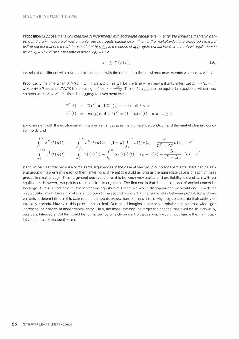
Proposition Suppose that a unit measure of incumbents with aggregate capital level v

– I

enter the arbitrage market in peri-

od 0 and a unit measure of new entrants with aggregate capital level v

– E

enter the market only if the expected profit per

unit of capital reaches the J

+

threshold. Let {v

–

(t)}∞t=0

is the series of aggregate capital levels in the robust equilibrium in

which v

–

0

= v

– E

+ v

– I

and τ the time in which v

–

(t) = v

– E

.If

(20)

the robust equilibrium with new entrants coincides with the robust equilibrium without new entrants where v

–

0

= v

– E

+ v

– I

.

Proof Let κ the time when J′ (v(k)) = J

+

. Thus κ ≤ τ This will be the time when new entrants enter. Let ∆v

–

= v

–

(κ) – v

– E

,

where ∆v

– ≥ 0 because J′ (v(t)) is increasing in t. Let . Then if {x

–

(t)}∞t=0

are the equilibrium positions without new

entrants when v

–

0

= v

– E

+ v

– I

, then the aggregate investment levels

are consistent with the equilibrium with new entrants, because the indifference condition and the market clearing condi-

tion holds and

It should be clear that because of the same argument as in the case of one group of potential entrants, there can be sev-

eral group of new entrants each of them entering at different threshold as long as the aggregate capital of each of these

groups is small enough. Thus, a general positive relationship between new capital and profitability is consistent with our

equilibrium. However, two points are critical in this argument. The first one is that the outside pool of capital cannot be

too large. If (20) did not hold, all the increasing equilibria of Theorem 1 would disappear and we would end up with the

only equilibrium of Theorem 2 which is not robust. The second point is that the relationship between profitability and new

entrants is deterministic in this extension. Incumbents expect new entrants, this is why they concentrate their activity on

the early periods. However, this point is not critical. One could imagine a stochastic relationship where a wider gap

increases the chance of larger capital entry. Thus, the larger the gap the larger the chance that it will be shut down by

outside arbitrageurs. But this could be formalized by time-dependent q values which would not change the main quali-

tative features of the equilibrium.

MAGYAR NEMZETI BANK


In this paper I present an analytically tractable general equilibrium model of dynamic arbitrage. In our model arbitrage

opportunities arise because of a temporary pressure on local demand curves of two very similar assets traded in seg-

mented markets. The temporary demand pressure is present for an uncertain, arbitrarily long time span, but disappears

in finite time with probability one. Risk-neutral arbitrageurs can take positions in both local markets, and have to decide

how to allocate their limited capital across uncertain future arbitrage opportunities. This allocation – together with the

uncertain duration of the local demand pressure – determines the future distribution of the price gap between the two

assets. Hence, the individually optimal intertemporal allocation of capital and the distribution of future arbitrage oppor-

tunities are determined simultaneously in equilibrium.

I argued that competition among arbitrageurs with limited capital transforms the dynamic properties of arbitrage prices.

In particular, even if the fundamental process is riskless in the sense that the price gap could never widen, arbitrageurs’

activity introduces potential losses. Interestingly, the intuition behind this result is of the same type as the text-book argu-

ment of why unconstrained arbitrageurs eliminate price discrepancies. There, price discrepancies cannot exist, because

they are so attractive for arbitrageurs that they would eliminate them. I showed that when arbitrageurs are financially con-

strained, there cannot be any time period when there are no potential losses, because this would be a too attractive arbi-

trage opportunity. Arbitrageurs would increase their positions in these periods relative to other periods, which would cre-

ate potential losses.

Importantly, I highlighted that our mechanism is not based on amplification of an external shock. In the robust equilibri-

um, there are no exogenous reasons which would result in losses for arbitrageurs in any states of the world. Arbitrageurs

total losses are created endogenously. In a calibrated example, I showed that in this case, arbitrageurs lose most of their

capital with positive probability in a relatively short time.

The model illustrates that the presence of price gaps between fundamentally very similar assets does not necessarily

indicate the lack of arbitrage activity, even if these gaps are occasionally substantial. In the robust equilibrium, arbi-

trageurs with limited capital never fully eliminate price gaps. The main effect of their activity is different. They transform

the dynamics of the price gap so it will move in a much less predictable way. Thus the arbitrage opportunity becomes

much less profitable. Decreasing the predictability of price differentials is the way how positive expected profits are trad-

ed away by arbitrageurs.

The simplicity of our framework provides the potential of wide applicability to different problems related to limited arbi-

trage. In Kondor (2006), I demonstrate this potential by building an extension of career concerns on top of our structure.

As future work I consider the applicability of our model to a multi-asset set up to analyze contagion across markets and

the effects of flight-to-quality and flight-to-liquidity in times of market depression. I believe that our mechanism will shed

more light on these issues.


6. Conclusion

[1] ABREU, D., BRUNNERMEIER, M., 2002. Synchronization risk and delayed arbitrage, Journal of Financial Economics, 66,

341-360.

[2] ABREU, D., BRUNNERMEIER, M., 2003. Bubbles and crashes, Econometrica, 71(1), 173-204.

[3] AGARWAL, V., NAIK, N. Y., 2004. Risks and portfolio decisions involving hedge funds, Review of Financial Studies,

17(1), 63-98.

[4] BASAK, S., CROITORU, B., 2000. Equilibrium mispricing in a capital market with portfolio constraints, Review of

Financial Studies 13, 715-748.

[5] BERNARDO, A., WELCH, I., 2004. Liquidity and financial market runs, Quarterly Journal of Economics 119(1), 135-158.

[6] BRUNNERMEIER, M. K., PEDERSEN, L. H., 2005. Predatory trading, Journal of Finance, 60(4), 1825-1863.

[7] DANIELSSON, J., SHIN, H.S., 2002. Endogenous risk, LSE, mimeo.

[8] DANIELSSON, J., SHIN, H.S., ZIGRAND, J-P., 2004. The impact of risk regulation on price dynamics, Journal of Banking

and Finance, 28, 1069-108.

[9] DIXIT, A., PINDYCK, R., 1994. Investment under uncertainty, Princeton: Princeton University Press.

[10] EDWARDS, F., 1999. Hedge funds and the collapse of long-term capital management, Journal of Economic

Perspectives 13, 189-210.

[11] ENGLE, R. F., ROSENBERG, J. V., 2002. Empirical pricing kernels, Journal of Financial Economics, 64, 341-372.

[12] FROOT, K. A. DABORA, E. M., 1999. How are stock prices affected by the location of trade?, Journal of Financial

Economics, 53(2), 189-216.

[13] FROOT, K., SCHARFSTEIN, D., STEIN, J., 1993. Risk management: coordinating corporate investment and financing poli-

cies, Journal of Finance, 48, 1629-1658.

[14] GROMB, D., VAYANOS, D., 2002. Equilibrium and welfare in markets with financially constrained arbitrageurs, Journal

of Financial Economics, 66, 361-407.

[15] HOLMSTRÖM, B., TIROLE, J., 2001. LAPM: A liquidity-based asset pricing model, Journal of Finance, 56(5), 1837-1867.

[16] KONDOR, P., 2006. Career concerns and dynamic arbitrage, LSE, mimeo.

[17] KUMAR, M. S., PERSAUD, A., 2001. Pure contagion and investors shifting risk appetite: analytical issues and empirical

evidence, IMF Working Papers: 01/134.

[18] KYLE, A. S., XIONG, W., 2001. Contagion as a wealth effect, Journal of Finance, 56, 1401-1440.

[19] LAMONT, O. A., THALER, R. H., 2003. Anomalies: the law of one price in financial markets, Journal of Economic

Perspectives, 17(4), 191-202.

[20] LIU, J., LONGSTAFF, F., 2004. Losing Money on Arbitrage: Optimal Dynamic Portfolio Choice in Markets with Arbitrage

Opportunities, Review of Financial Studies, 17(3), 611-641.

[21] LOEWENSTEIN, R., 2000. When genius failed: the rise and fall of long-term capital management, New York, Random

House.

[22] LUCAS, R. E. JR., 1978. Asset prices in an exchange economy, Econometrica, 46(6), 1426-1445.

[23] MACKENZIE, D, 2003. Long-Term Capital Management and the sociology of arbitrage, Economy and Society 32(3),

349-380.

[24] MERTON, ROBERT C., 1971. Optimum consumption and portfolio rules in a continuous-time model, Journal of

Economic Theory, 3, (December):373-413. Reprinted in Merton (1992, Ch. 5).

[25] MERTON, ROBERT C., 1992. Continuous-time finance. Rev. ed. Oxford, U.K.: Basil Blackwell.

[26] MORRIS, S., SHIN, H. S., 2004. Liquidity black holes, Review of Finance, 8, 1-18.

[27] NIEUWERBURGH, S. VAN, VELDKAMP, L., 2005. Information acquisition and portfolio under-diversification, NYU, mimeo.

[28] PLANTIN, G., SHIN, H. S., 2005. Weight of Money Pricing and Speculative Dynamics, LSE, mimeo.

[29] SHLEIFER, A., VISHNY, R., 1997. The limits of arbitrage. Journal of Finance 52, 35-55.

[30] XIONG, W., 2001. Convergence trading with wealth effects. Journal of Financial Economics 62, 247-292.

[31] ZIGRAND, J-P., 2004. General equilibrium analysis of strategic arbitrage, Journal of Mathematical Economics, 40(8),

923-952.


References

A.1. MICROFOUNDATION OF LOCAL TRADERS’ BEHAVIOR

In this appendix I provide a possible microfoundation of local traders’ behavior which is consistent with Assumptions 1-

7. First I show that a standard OLG set-up with general utility functions is sufficient to satisfy Assumptions 1 and 2 and I

give the necessary restriction on the utility function which makes the structure consistent with Assumption 6. For

Assumptions 3-7, more structure is needed. Thus I present an example with CARA utilities which satisfy all assumptions.

The reader may observe that Assumption 7 is the most demanding. It is virtually equivalent with the requirement of the

negative exponential utility function in a representative agent framework. Although it might seem too restrictive, this

Assumption is not critical for the main results of the paper. It only simplifies the analysis enormously.

Let us suppose that each trader lives for a fixed interval of ∆d

and a new generation of traders is born in each time

instant.

25

As the assets pay a dividend once in each ∆d

interval, all traders receive dividend payments exactly once in

his lifetime. Each trader receives a lifetime endowment and makes a buy-and-hold investment decision when born, and

liquidates her investment and consumes the proceeds just before she dies. Her lifetime endowment, n

i

(t) consists of a

constant wage, n, and a non-tradable stochastic component which is correlated with the pay-off of the risky asset, R (td

).

In particular, the stochastic component pays w

i

R (td

) units at each t if the window is open. Hence, the value of her

endowment just before she dies will be

and ωB

= ω′ ≠ ωA

= ω′′. The window closes when the stochastic component disappears, i.e., ωA

= ωB

= 0.

Each young trader born at time t on island i makes the investment decision of buying θ i

(t) units of the risk asset when

born,. In time t + ∆t when old, she liquidates her investment and consume her total income: the value of her endowment

plus the proceeds of her investment decision. Each of them values her consumption according to a standard, strictly

increasing and concave utility function u (⋅). Hence, an i-trader, i = A,B, born at t in a window solves the problem

(21)

where the notation is the same as in the main text. The first order condition of this problem implicitly determines the

inverse demand curves p

i

(t) = d

i

(θ i

(t), p

i

(t + ∆t), p

c

(t + ∆t)) as long as the window is open. Note that this demand curve

is a special case of (1), as it depends only on one future price

Here, I endogenize the price when the window is closed, p

c

(t). I assume that windows can reopen but only after staying

closed at least for an interval of ∆d

. Hence, the window can change its state only once in each trader’s lifetime. The new

window will be one of two types. It will be either the same as the first one, or it can be a reverse window, where the roles

of the two group of traders are reversed, i.e., ωB

= ω′′ ≠ ωA

= ω′. Conditional on a closed window, a new window of each

type opens with probability in each time instant. This symmetric structure ensures that arbitrageurs do not have any

motivation to trade when the window is closed, which is consistent with the main text. Hence, when the window is closed,

traders born in period t solve a very similar problem to (21):


Appendix

25

Our OLG formulation is a simplifying assumption to keep our model tractable. It is not necessary for our story to go through. For example, infinitely lived

agents of Lucas (1978) would be consistent with the intuition. However, this would make the model much less tractable as in this case asset prices would

depend on both future and present consumption, hence they depend on past, present and future asset-holding. This would complicate the analysis with-

out providing virtually any added value.

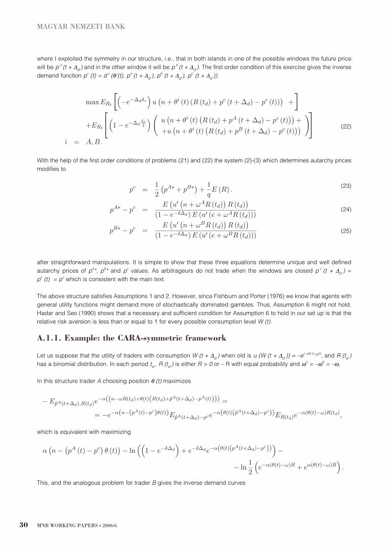
where I exploited the symmetry in our structure, i.e., that in both islands in one of the possible windows the future price

will be p

A

(t + ∆d

) and in the other window it will be p

B

(t + ∆d

). The first order condition of this exercise gives the inverse

demand function p

c

(t) = d

c

(θ i

(t), p

A

(t + ∆d

), p

B

(t + ∆d

), p

C

(t + ∆d

)).

(22)

With the help of the first order conditions of problems (21) and (22) the system (2)-(3) which determines autarchy prices

modifies to

(23)

(24)

(25)

after straightforward manipulations. It is simple to show that these three equations determine unique and well defined

autarchy prices of p

A

*, p

B

* and p

c

values. As arbitrageurs do not trade when the windows are closed p

c

(t + ∆d

) =

p

c

(t) = p

c

which is consistent with the main text.

The above structure satisfies Assumptions 1 and 2. However, since Fishburn and Porter (1976) we know that agents with

general utility functions might demand more of stochastically dominated gambles. Thus, Assumption 6 might not hold.

Hadar and Seo (1990) shows that a necessary and sufficient condition for Assumption 6 to hold in our set up is that the

relative risk aversion is less than or equal to 1 for every possible consumption level W (t).

A.1.1. Example: the CARA-symmetric framework

Let us suppose that the utility of traders with consumption W (t + ∆d

) when old is u (W (t + ∆d

)) = –e

(–aW (t+∆d))

, and R (td

)

has a binomial distribution. In each period td

, R (td

) is either R > 0 or – R with equal probability and ωA

= –ωB

= –ω.

In this structure trader A choosing position θ (t) maximizes

which is equivalent with maximizing

This, and the analogous problem for trader B gives the inverse demand curves

MAGYAR NEMZETI BANK


(26)

Thus, the structure is symmetric in the sense of Assumption 7.

The autarchy prices are given by

Because of p

A

(t) – p

c

= p

c

– p

B

(t) for any θ (t), θ–

= θ–

(p

A

t+1

+ p

B

t+1

) the position which eliminates the gap between current

prices for given future prices, is given as the unique and positive solution of

θ–

is well defined and positive, because the left hand side is a positive and monotonically decreasing function in θ–

while

the right hand side is monotonically increasing in θ–

and at θ–

= 0, the right hand side is larger than the left hand side.

Hence, Assumption 3 is satisfied. As the domain of right hand side of (26) contains R

+

for both arguments, Assumption

4 is also satisfied.

I show now that Assumption 5 holds for demand curve (26). I have to demonstrate that if θ–

+

is a solution of the equation

(28)

for a given g

+

then g

+

> g* implies θ +

< 0 and g

+

< 0 implies θ +

> 0. Let us start with the first case. Observe that the right-

hand side is a monotonically increasing function of θ +

while the right hand side is monotonically decreasing in θ +

for all

g

+

. We know from the definition of g* that if g

+

= 0 then θ +

= 0 Thus, if g

+

> g* then

Consequently, if g

+

> 0 θ +

must be negative to make the two sides of (28) equal. Similarly, g

+

= 0 and θ +

= ω satisfies

(28). But if g

+

< 0

Thus, if g

+

< 0, then θ +

must be larger than ω to make the two sides of (28) equal.

The last step is to check whether the relative risk aversion is less then or equal to 1 in the relevant range of θ ∈ [0, θ–

max

]

and gt+1

∈ [0,g*] . This implies that

has to hold for all R (td

) and θ ∈ [0, θ–

max

] and gt+1

∈ [0,g*] . As the supports of all variables on the right hand side are

bounded, there must be a small enough α which makes the inequality hold.

APPENDIX


A.2. PROOFS

Proof The interior solutions of the dynamic system are characterized by the differential equations First, let us check

whether corner solutions are possible. In a corner solution, there is at a time T when the aggregate budget constraint

binds and arbitrageurs cannot take positions. However, if v

–

(T) = 0, v

–

(T + τ) for all τ ≥ 0, because arbitrageurs cannot

realize gains without taking positions. Hence, if such a period existed, x

–

T+τ = 0 and gt+1

∈ [T + τ] = 0 for τ ≥ 0 as in

autarchy. But observe, that the expected marginal profit in autarchy is infinity as investing one unit in T would give

but g

⋅= 0. Which is a contradiction as it would imply that arbitrageurs would not save capital for a period with infinite mar-

ginal profit. Thus we have only interior solutions.

By standard methods the general solution of the non-homogenous linear differential equation of (8) is

where c1

is a constant. Plugging in the general solution of (8) into (7) gives the homogenous linear differential equation

with the general solution of

(29)

where c2

is a constant. Thus, limt→∞ g (t) = and g (0) = .

There is evidently an equilibrium, if g (t) = 0 for all t.This satisfies all the conditions with c1

= c2

= 0 and it also satisfies

the and the budget constraint for this case

(30)

To find the other solutions, note that form the construction of the system, g (t) and g

⋅(t) must have the same sign.

Otherwise the gap can move only in one direction and arbitrageurs have a safe profit opportunity. This would make them

to increase their positions without bounds so g (t) would reach 0 by Assumption 3. Thus, c1

> 0.

Let us suppose first that c2

< 0. In this case, g (t) would be always negative, monotonically increasing and would con-

verge to the negative level . Let us suppose that there exist a {x

–

(t)}∞t=0

which supports this path. Because of the conti-

nuity of f (x

–

t

,g (h)h>t

), there must be a large enough T that for any T + τ, the market clearing aggregate investment lev-

els {x

–

(t)}∞t=T+τ implied by the market clearing condition

would not change sing. As the limit of this series must be given by Assumption 5 implies that

x

–

(T+τ) is positive for all τ ≥ 0. In this case the potential loss in each period on each unit is hence, the budget constraint

has the form of g (T+τ)

(31)

MAGYAR NEMZETI BANK


But – as neither x

–

(t) nor g (t) converges to 0 – the left hand side is not convergent which is a contradiction. Analogous

arguments rule out the possibility of c2

> c1

g* where the aggregate positions are negative by Assumption 5 at least after

a fixed time T.

Thus, the only possibility that = g∞ ∈ [0, g*]. In this case all g (t) are positive and g (t) is monotonically increasing. From

g (0) = g0

and limt→∞ g (t) = g∞ we get , thus

(32)

(33)

Observe, that if we compare local traders’ distribution of pay-offs in the autarchy case and when 0 < g (t) < g* is monot-

onically increasing, by Assumption 6, we have to conclude that x (t) ∈ (0, θ–

max

) for all t. Thus the largest loss in each peri-

od is g

⋅(t). As the expected instantaneous profit is positive in each period, the budget constraint has to be strict:

(34)

The last step is to find a g0

as a function of ν–

0

for a given g∞ to satisfy the budget constraint (34). The series {g (t)}∞t=0

will

give the series x

–

(t) by the market clearing condition. First note that for a given g∞ if {g (t)}∞t=0

is the series with g (0) = g0

and {g

+

(t)}∞t=0

is the series with a g (0) = g

+

0

where g0

< g

+

0

then the two series differ only in their starting points, i.e., there

is a h that g

+

(t) = g (t+h) for all t.To see this, observe that as g (t) is continuous and monotonically increasing between

g0

and g∞ there must be a h that g (h) = g

+

0

. But then

This implies that

thus ∫ ∞

0

x

–

(t) g

⋅(t) is monotonically decreasing in g

0

for any fixed g∞ . Consequently, if

for any ν–

0

∈ (0, ν–

0

max,g∞) there exists a single g

0

that

Proof of Theorem 3 Interior solutions of the dynamic system with m > 0 are given by

(35)

(36)

APPENDIX


The general solution is

(37)

(38)

It is clear that the budget constraint can only converge if limt→∞ x

–

(t) = 0 so imt→∞ x

–

(t) = g*. As is

not convergent, there cannot be an interior solution for all t. Hence, by large enough T arbitrageurs will lose all their cap-

ital and we must have a corner solution of x

–

(T+τ) = 0 and g (T+τ) = g* for τ ≥ 0. As this implies a stationary environment

and δ > 0, in this case arbitrageurs would choose to invest all their capital in time T if they had any. Thus,

and . From g (T) = g*.

Consequently, for all 0 ≥ t > T

Observe that

Similarly to the proof of Theorem 1, we know that there is {x

–

(t)}∞t=0

∈ (0, θ–

max

) which satisfy the market clearing condition

g (t) = f (x

–

(t), g (h)h>t

) for all t. The last step is to find T. By definition of T, we know that

(39)

must hold. Since g (t) depends on time only through T – t the left hand side of (39) is monotonically increasing in T. As

and

for any ν–

0

> 0, there must be a unique T which satisfies (39).

Proof Theorem 4 As I showed in the proof of Theorem 1, the robust equilibrium is given by the general solution of differ-

ential equations (7)-(8), (29) and two boundary conditions. The first one is limt→∞ g (t) = g* which gives c

2

= g*c1

. The

second one is the budget constraint (34). In the proof, I defined g0

in terms of c1

and used (34) to pinned down g0

. An

equivalent step is to pin down c1

by (34). Observe also that the unique equilibrium when m > 0 can be given by the fol-

lowing steps. We know that for all t ≤ T the general solution is

(40)

MAGYAR NEMZETI BANK


where I added subscript m to the constants c

m

1

and c

m

2

to distinguish from the corresponding constants in the robust equi-

librium. Instead of expressing c

m

1

from the boundary condition

we can equivalently express T as

Substituting T into (40), the boundary condition g (T) = g* gives

(41)

Finally, c

m

1

is pinned down by the modified budget constraint after substituting (41) into (40):

(42)

Observe that as m → 0, the general solution (38) converges to (29), limm→∞ c

m

2

= c

m

1

g*, limm→0

T = ∞, thus the left hand

side of (42) converges to the left hand side of (34). Consequently, limm→0

c

m

1

= c1

and the equilibrium with m >0 must

converge to the robust equilibrium.

APPENDIX


MNB Working Papers 2006/6

Risk in Dynamic Arbitrage: Price Effects of Convergence Trading

Print: D-Plus

H–1033 Budapest, Szentendrei út 89–93.

Date post:	06-Sep-2018
Category:	Documents
Upload:	phamthuy
View:	224 times
Download:	0 times

MNB Working Papers 2006/6. · Cochrane, Darrell Duffie, Zsuzsi Elek, Antoine Faure-Grimaud, Miklós...

Documents