Connected Dominating Set forTopology Control in Ad HocNetworks
Bo Han,1 Lizhuo Zhang,2 and Weijia Jia2
1 Department of Computer Science, University of Maryland, College Park, MD2 Department of Computer Science, City University of Hong Kong, Kowloon, Hong Kong
2.1 Introduction 262.2 Related Work 282.3 Network Assumptions and Preliminaries 292.4 Area-Based CDS Formation Algorithm 302.5 Experimental Simulations 362.6 Conclusion and Future Work 39Acknowledgments 40References 41
2.1 INTRODUCTION
In wireless ad hoc networks that are formed by autonomous mobile devices commu-nicating through radio, topology control plays an important role in the performance ofthe protocols used in the network, such as routing, clustering, and broadcasting. Thereare two approaches for topology control in ad hoc networks—transmission range con-trol and hierarchical topology organization (clustering). The goal of this technique isto control the topology of the graph representing the communication links betweennetwork nodes, with the purpose of maintaining some global graph property (such as
connectivity) while reducing energy consumption. Moreover, topology control has thepositive effect of reducing contention when accessing wireless channels. In general,when the nodes’ transmission ranges are relatively short, many nodes can transmitsimultaneously without interfering with each other, and the network capacity is thusincreased. Ideally, the nodes’ transmission ranges should be set to the minimum valuesuch that the communication graph is connected.
As mentioned above, transmission range control is a general approach for topol-ogy control in ad hoc networks. The construction of hierarchical topology (clustering)is another effective solution. Cluster-based constructions are commonly regarded asa variant of topology control in the sense that energy-consuming tasks can be sharedamong the members of a cluster. The basic idea of clustering is to group the networknodes that are in physical proximity to provide the network with a logical organi-zation that is smaller in scale, and hence simpler to manage [6]. The notion ofcluster organization has been investigated for ad hoc networks since their appear-ance. Baker et al. [27] introduced a fully distributed linked cluster architecture anddemonstrated adaptability of the network to topological changes. With the adventof multimedia communications, the use of the cluster has been revisited by Gerlaand Tsai [22] with the emphasis on the allocation of resources to support the multi-media traffic in ad hoc networks. Basagni proposed a distributed clustering algo-rithm that generalizes these clustering protocols in that the choice of the cluster-head is performed based on a generic “weight” associated with a node [17]. Thisattribute basically expresses how fit that node is to become a clusterhead. Clus-tering algorithms have also been proposed explicitly for wireless sensor networks.Among these protocols, one of the first is the low-energy adaptive clustering hie-rarchy (LEACH) protocol presented in Ref. [28]. LEACH uses randomized rotationof the clusterheads to evenly distribute the energy load among the sensors for networklongevity.
Although wireless ad hoc networks have no physical infrastructure, it is naturalto construct clusters through connected dominating set (CDS) formation. In general,a dominating set (DS) of a graph G = (V, E) is a subset V ′ ⊂ V such that each nodein V − V′ is adjacent to at least one node in V′, and a connected dominating set is adominating set whose induced subgraph is connected. It has been pointed out that“the most basic clustering that has been studied in the context of ad hoc networks isbased on dominating sets” [4]. Moreover, the CDS can also play an important role inmessage broadcasting in ad hoc networks [3]. Unfortunately, the dominating set andconnected dominating set problems have been shown to be NP-complete [5]. Evenfor a unit disk graph (UDG) [1], the problem of finding a minimum CDS (MCDS) isstill NP-complete [7].
This chapter presents a novel distributed algorithm, named the Area algorithm,for CDS formation in wireless ad hoc networks. In this algorithm, we partition thenodes into different areas and selectively connect two dominators that are two orthree hops away. Note that the clusterheads in most clustering algorithms [17, 22]usually form a DS. Since they focused on clusterhead selection, the clusterheads andgateways (selected to connect two clusterheads) construct a CDS with a relativelylarge size. Thus, our contribution mainly lies in that we introduce the Area concept to
28 Connected Dominating Set for Topology Control in Ad Hoc Networks
significantly reduce the number of connectors that connect two neighboring domina-tors, therefore reduce the size of final CDS.
The rest of the chapter is organized as follows. Section 2.2 introduces the re-lated work. Section 2.3 describes the network assumption and some preliminaries. InSection 2.4, we present our novel distributed CDS formation algorithm and give theperformance analysis. Section 2.5 presents the simulation results. We point out futuredirections and summarize major results in Section 2.6.
2.2 RELATED WORK
In this section, we discuss related work with respect to topology control in two cat-egories: transmission range control and hierarchical topology organization (in thecontext of connected dominating set formation).
2.2.1 Transmission Range Control
Most of the existing topology control algorithms select a less-than-normal transmis-sion range (also called the actual transmission range) while maintaining network con-nectivity. Centralized algorithms [26] construct optimized solutions based on globalinformation and, therefore, are not suitable in wireless ad hoc networks. Some prob-abilistic algorithms [8] adjust transmission range to maintain an optimal number ofneighbors. However, probabilistic algorithms do not provide hard guarantees on net-work connectivity. Most of the localized topology control algorithms use nonuniformactual transmission ranges computed from one-hop information (under the normaltransmission range) and take advantage of some original research topics in computa-tional geometry, such as the minimum spanning tree [20], the Delaunay triangulation[19], or the relative neighborhood graph [21]. Most of these contributions mainlyconsidered energy efficiency of paths in the resulting topology. The CBTC algorithm[18] was the first construction to focus on several desired properties. A nice literaturereview of transmission range control can be found in Ref. [4].
2.2.2 Connected Dominating Set
Das et al. proposed a MCDS-based routing algorithm for wireless ad hoc networks [2].This algorithm is a distributed version of Guha and Khuller’s centralized algorithm tocalculate a connected dominating set [10]. The algorithm proposed by Wu and Li firstfinds a connected dominating set and then prunes certain redundant nodes from theCDS using two rules (Rule 1 and Rule 2) [11]. In the first phase, each node is markedtrue (dominator) if it has two unconnected neighbors. According to Rule 1, a markednode can unmark itself if its neighbor set is covered by another neighboring markednode. According to Rule 2, a marked node can unmark itself if its neighborhood iscovered by two other neighboring directly connected marked nodes. The combinationof Rules 1 and 2 is fairly efficient in reducing the size of CDS. This algorithm is fully
2.3 Network Assumptions and Preliminaries 29
localized, but does not guarantee a good approximation ratio. Hereafter, this algorithmis referred to as Rule 1&2 (so named for the two pruning rules). Stojmenovic et al.also presented a distributed construction of CDS in the context of clustering andbroadcasting [12]. The solution proposed in Ref. [23] relies on all nodes having acommon clock and requires two-hop neighbor information. In CEDAR [13], a virtualinfrastructure called the core is constructed to approximate a minimum dominatingset (not connected) of the underlying network.
For distributed clustering algorithm, it is undesirable to have neighboring clus-terheads [17]. It is also undesirable to have one-hop away neighboring dominators indominating set formation. This leads to the well-known concept of maximal indepen-dent set (MIS). An independent set of graph G = (V, E) is a subset S ⊂ V such thatfor any pair of vertices in S, there is no edge between them. Obviously, an MIS S isalso an independent DS. The two heuristic algorithms proposed by Alzoubi et al. [14]take advantage of the property of MIS, thus may guarantee a constant approximationratio of 8 and 12, respectively. Although these two algorithms are distributed, theyare not localized. To address the problem of nonlocalized computation, Alzoubi et al.also proposed a message-optimal localized algorithm with linear time and messagecomplexity [15]. This algorithm can be briefly described as two phases. In the firstphase, an MIS is constructed. As mentioned above, this MIS is also a DS. In thesecond phase, each dominatee identifies the dominators that are at most two hopsaway from itself and broadcasts this information. Using such information from allneighbors, each dominator identifies a path to each dominator that is at most threehops away from itself and informs all nodes in this path to become the connectorsand join the final CDS. The approximation ratio of this algorithm is bounded by 192.For simplicity, we call this algorithm AWF in the following. Recently, Wang et al.proposed an efficient distributed method to construct a low-cost weighted minimumconnected dominating set [24].
2.3 NETWORK ASSUMPTIONS AND PRELIMINARIES
In this chapter, we assume that an ad hoc network comprises a group of nodes com-municating with the same transmission range. Scheduling of transmission is the re-sponsibility of the MAC layer. Each node has a unique ID and each node knows theID and degree of its neighbors, which can be achieved through periodically broad-casting “HELLO” messages by each node. Since the emphasis of this chapter ison the CDS formation, we do not consider the node mobility. We call the nodesin the dominating set dominators, the nodes not in the dominating set dominatees,and the nodes that connect two or three hops away dominators connectors. Espe-cially, we call the connectors that connect dominators two and three hops away one-hop connector and two-hop connector, respectively. Next, we give some well-knownpreliminaries.
Preliminary 2.1. By building a dominating set through MIS construction, for everynode u, the number of dominators inside the disk centered at u with radius k-unit isbounded by a constant lk .
30 Connected Dominating Set for Topology Control in Ad Hoc Networks
Proof. Alzoubi et al. gave a proof through calculation of lk < (2k + 1)2 − 1 [15]. Whenk = 2, 3, we have lk = 23, 47. Recently, Li et al. have proved that l3 = 42 [16].
Preliminary 2.2. Let G be a UDG and opt be the size of a minimum CDS for G, thenthe size of any MIS for G is at most 3.8 × opt + 1.2.
The proof of this preliminary bounds the size of any MIS in G and can be foundin Ref. [9].
Preliminary 2.3. In a DS, the maximum distance to another closest dominator fromany dominator is 3.
Proof. By contradiction. Assume that the maximum distance from a dominator u tothe closest dominator v is 4, and the shortest path between u and v is {u, x, y, z, v}.According to the definition of dominating set, node y must have a dominator, say w,which is one hop closer (three hops) to u than v. This contradicts the assumption thatv is the closest dominator to u.
2.4 AREA-BASED CDS FORMATION ALGORITHM
2.4.1 Overview
A well-known method for building connected dominating set is to construct an MISfirst, which is also a dominating set, and then add some connectors to guarantee theconnectivity. This method was utilized by Alzoubi et al. [14, 15]. The algorithms inRef. [14] were implemented by first electing a leader r among the nodes, which wasgoing to be the root of a spanning tree T. The approximation ratios of these algorithmsare attractive; however, the message complexity O(n log n), which is bounded by thedistributed leader election, is quite high in real practice [6]. Moreover, they are notlocalized algorithms. The algorithm presented in Ref. [15] has an optimal messagecomplexity O(n), but it connects any pair of dominators (at most three hops away) byadding one or two connectors. Consequently, the resultant CDS has a relative largesize with some redundant connectors.
Our main objective of this Area algorithm is to reduce the size of CDS. Weuse the most-valued nodes as the metric to select the nodes among all nodes in thegraph for the CDS. The value of a node is a performance-related characteristic suchas node ID, node degree, or remaining battery life. In this chapter, we define twokinds of most-valued nodes, one is the nodes with the minimum ID among all thecandidates of dominators or connectors (the resulting Area algorithm is called MinID) and the other is the nodes with the maximum degree among all the candidates(hence, called Max Degree). In the following description of Area algorithm, we willuse node degree as the selection metric. We stress that the proposed algorithm canalso be easily extended to support other node values.
2.4 Area-Based CDS Formation Algorithm 31
2.4.2 Max Degree Algorithm
Define the rank of node u to be an ordered pair of (δu , idu ), where δu is the nodedegree and idu is the node ID of u. We say that a node u with rank (δu , idu ) has ahigher order than a node v with rank (δv , idv ) if δu > δv , or δu = δv and idu < idv . Eachnode is in one of the four states: unmarked, dominatee, dominator, or connector. Eachnode is initially in an unmarked state and subsequently enters either the dominatee ordominator state. The connector state can only be entered from the dominatee state.In this Area algorithm, we partition the nodes into different areas and each area issupposed to have a unique area ID. Thus, each node is also assigned an area ID toindicate which area it belongs to. For simplicity of description, we first give somedefinitions below.
Definition 2.1 (Seed Dominator). A dominator that has the highest rank among itsone-hop neighbors.
Definition 2.2 (Nonseed Dominator). A dominator that has at least one one-hopneighbor with higher rank.
Definition 2.3 (Border Dominator). A dominator that has two or three hops awayneighboring dominators with different area IDs.
2.4.2.1 Area Formation
First, an unmarked node u with the highest rank among its unmarked one-hop neigh-bors becomes a dominator and broadcasts a DOMINATOR message to its neighbors.Note that such a node does exist in the beginning. After receiving a DOMINATORmessage, a node, say v, changes its state to be the dominatee if its current state isunmarked. If it is the first time that v receives a DOMINATOR message, v also broad-casts a DOMINATEE message to its neighbors. The same procedure is repeated untileach node becomes either a dominator or a dominatee.
In fact, seed dominators are the starting points of the process of these MIS-basedalgorithms and they are the cores of the areas. The ID of a seed dominator automat-ically becomes the ID of the corresponding area. During the area formation, we addan item, Area ID, into the DOMINATOR message to indicate the area that the domi-nator belongs to. When an unmarked node receives the first DOMINATOR message,it becomes a dominatee of the area indicated in this message. Each dominatee alsoinserts its area ID into the DOMINATEE message that it broadcasts to its neighbors.Then every nonseed dominator can know the area it belongs to from its neighboringdominatees. If neighboring dominatees have different area IDs, the nonseed domina-tor can arbitrarily select one area to join. The nodes with the same area ID form anarea eventually.
32 Connected Dominating Set for Topology Control in Ad Hoc Networks
2.4.2.2 Area Connection
After the nodes are partitioned into different areas, the following steps are executedby the related nodes:
1. Each dominatee broadcasts a ONE-HOP-DOMINATOR message that containsall node IDs and area IDs of its one-hop away dominators.
2. After receiving a ONE-HOP-DOMINATOR message, each node knows itstwo-hop away dominators and the corresponding neighbors to connect thesedominators. The neighbor with higher rank has the priority to be chosen as aconnector (maybe NOT the connector in the final CDS).
3. Upon reception of the ONE-HOP-DOMINATOR message from all its neigh-boring dominatees, a dominatee broadcasts a TWO-HOP-DOMINATOR mes-sage that contains all node IDs and area IDs of its two-hop away dominators.
4. After receiving a TWO-HOP-DOMINATOR message, each dominator knowsits three-hop away neighboring dominators and the relevant neighbors to con-nect these dominators. Also, the neighbor with higher rank has the priority tobecome a connector.
After having the knowledge of all the two-hop and three-hop away neighboringdominators, each dominator can know whether it is a border dominator. Dominatorsinside an area try to connect only their two-hop away neighboring dominators withlarger IDs by selecting one connector. Border dominators connect only one two-hop or three-hop away neighboring dominator with larger ID in an adjacent area byselecting one or two connectors. That is, if a border dominator has connected to atwo-hop away neighboring dominator in an adjacent area, it will not try to connect thethree-hop away neighboring dominator in the same adjacent area. Then the dominatingset is constructed through a sweep of the network spreading outward from the seeddominators. To illustrate the algorithm, Figure 2.1 gives an example of the CDSformation using Max Degree algorithm.
2.4.2.3 Example
In Figure 2.1, the IDs of nodes are labeled beside the nodes. Black nodes repre-sent the dominators, black nodes with outer circle represent the seed dominators,and gray nodes represent the connectors. A possible execution scenario is shown inFigure 2.1(b)–(d), as explained below.
1. Initially, all nodes are unmarked (Figure 2.1(a)).
2. Nodes 7 and 14 declare themselves as dominators, since they have the highestranks among their unmarked one-hop neighbors. These two dominators arealso seed dominators. After receiving a DOMINATOR message, nodes 5, 9,13, 15, 16, 20, 22, 23, 24, 25, 26, and 27 declare themselves as the dominateesand broadcast DOMINATEE messages (Figure 2.1(b)).
3. After receiving DOMINATEE messages from their neighbors, nodes 6, 10,18, 19, and 21 declare themselves as dominators and broadcast DOMINATOR
2.4 Area-Based CDS Formation Algorithm 33
7
8
6
5
4 3
2
1
27
26
24
23
2221
20
19
18
17
16
1513
12
14
11
10
9
25
(a) Initial topology
7
8
6
5
4 3
2
1
27
26
24
23
2221
20
19
18
17
16
1513
12
14
11
10
9
25
(b) Seed dominators selected
7
8
6
5
4 3
2
1
27
26
24
23
2221
20
19
18
17
16
1513
12
14
11
10
9
25
(c) More dominators selected
7
8
6
5
4 3
2
1
27
26
24
23
2221
20
19
18
17
16
1513
12
14
11
10
9
25
(d) Complete CDS formation
Figure 2.1 CDS construction by Max Degree algorithm.
messages. The reason is that all their neighbors with higher ranks became dom-inatees, thus their ranks become the highest among their unmarked neighbors.At this time, all the dominators form an MIS and there are two areas centeredat dominators 7 and 14, respectively. Suppose dominators 10 and 6 choose tojoin the areas with ID 7 and 14, respectively (Figure 2.1(c)).
4. After each dominatee broadcasts ONE-HOP-DOMINATOR and TWO-HOP-DOMINATOR messages, every dominator knows its two-hop and three-hopaway neighboring dominators. According to the definition, dominators 6, 10,and 14 know that they are border dominators. Finally, dominatees 22 and 24are selected to become connectors by dominator 7 to connect dominators 10,18, and 19; dominatee 27 is selected as connector by dominator 6 to connectdominator 14. Dominatee 17 is selected by dominator 6 to connect the twoadjacent areas. Obviously, all the black and gray nodes form a connected dom-inating set of the graph and the induced subgraph is indicated by the thickblack lines (Figure 2.1(d)).
Note that compared to dominatee 9 whose rank is (3, 9), dominatee 27 has a higherrank (4, 27), so it is selected by dominator 6 to connect dominator 14. Dominatee27 is also the only node that connects dominators 14 and 21. Since dominator 10has a two-hop away neighboring dominator (node 6) in the adjacent area, it will nottry to connect its three-hop away neighboring dominator (node 14) in the same area.From the above example, we can see that the benefit of using the area concept isthat dominators can selectively connect to their two or three hops away neighboringdominators, thus reduce the size of the final CDS.
34 Connected Dominating Set for Topology Control in Ad Hoc Networks
Figure 2.2 A sample network with 140 nodes: (a) entire network, (b) CDS by Rule 1&2, (c) CDS byAWF, (d) CDS by Min ID, and (e) CDS by Max Degree.
Figure 2.2 shows a comparison of our two Area algorithms, Min ID and MaxDegree with Rule 1&2 [11] and AWF [15]. We use a sample network with 200 nodes.The original topology of the network is depicted in Figure 2.2(a). Figure 2.2(b)–(e)shows the CDS generated by Rule 1&2 (Figure 2.2(b)), AWF (Figure 2.2(c)), MinID (Figure 2.2(d)), and Max Degree algorithms (Figure 2.2(e)), respectively. In thesefour figures, only nodes in the CDS and their induced graph are shown. The size ofthe CDS constructed by these four algorithms is 101 (Rule 1&2), 98 (AWF), 76 (MinID), and 55 (Max Degree), respectively. We can see that the CDS constructed by MaxDegree algorithm contains the least number of nodes, followed by Min ID algorithm.
2.4.3 Performance Analysis
In this subsection, we show the correctness, analyze the time and message complexityof the Area algorithm, and give the approximation ratio of this algorithm.
Theorem 2.1. The dominators and connectors selected by the Area algorithm forma CDS.
Proof. In this Area algorithm, it can be easily proved that each dominator has atleast one two-hop away neighboring dominator in the area it belongs to if there is
2.4 Area-Based CDS Formation Algorithm 35
any other dominator existing in the same area. To connect each pair of two-hop awaydominators, we can guarantee the connectivity inside these areas. Note that we alsoconnect two adjacent areas using at least one path; thus, this theorem is proved.
Theorem 2.2. The Area algorithm has both time and message complexity of O(n).
Proof. The time complexity of this algorithm is bounded by MIS construction thathas the worst time complexity O(n). The worst case occurs when all nodes are dis-tributed in a line and in either ascending or descending order of their ranks. The restof the process has time complexity at most O(n). Since each node sends a constantnumber of messages, the total number of messages is also O(n).
Theorem 2.3. Let G be a unit disk graph and opt be the size of a minimum CDSfor G, then the size of CDS constructed by this Area algorithm is within a constantapproximation ratio of opt.
Proof. From Preliminary 2.2, we know that the size of MIS is at most 3.8 ×opt + 1.2. Since each pair of nodes in MIS introduces at most two nodes to CDS,from Preliminary 2.1, the number of nodes in the CDS is at most (42×2/2 + 1) ×(3.8×opt + 1.2) = 163.4×opt + 51.6.
The density μ of graph can be calculated as
μ(r) = (nπr2)/A (2.1)
where n is the number of nodes in the graph, A is the area of the graph, and r is thetransmission range. Let D be the maximum density of packing of n equal circles in acircle. The upper bound of D is given in Ref. [25]:
D ≤ n[1 −
√3
2 +√
34 + 2
√3
π(n − 1)
]2 (2.2)
From (2.1) and (2.2), we can further refine l2 in Preliminary 2.1 to be 21. Rememberthat, in this Area algorithm, the dominators and one-hop connectors form a CDS inthe induced subgraph of each area. Let opt’ be the size of a minimum CDS for theinduced subgraph of an area. Through the similar analysis of Theorem 2.3, the sizeof CDS for an area is at most (21/2+1)×(3.8×opt′+1.2) < 44×opt′+14.
2.4.4 Discussion of Mobility Issues
Mobility management is an important research topic in wireless ad hoc networks andsometimes node mobility can have good effects on the protocol design. For example,epidemic routing [29] exploits rather than overcomes mobility to achieve a certaindegree of connectivity in occasionally partitioned networks; message ferrying is amobility-assisted approach that can provide efficient data delivery in sparse ad hoc
36 Connected Dominating Set for Topology Control in Ad Hoc Networks
networks where network partitions can last for a significant period [30]. However,node mobility is treated as undesirable for the CDS construction, since it will causeinconsistent local view. Dynamic topology change resulting from node mobility canbe handled by the methods proposed in Refs. [11, 15]. Generally, there are two kindsof mechanism: periodical reconstruction and on-demand update. Each method hasits own pros and cons. In the former scheme, the period of time elapses before thereconstruction is critical to the system performance. On-demand update is efficientin slight topology change and will lose its effectiveness when facing major topologychange. In our future work, we plan to integrate both of these two methods with theproposed Area algorithm to maintain the CDS for mobile ad hoc networks. However,how to update the topology efficiently while preserving the approximation quality isstill an open problem.
The next section gives extensive simulation study to verify the efficiency of thisArea algorithm in terms of the size of CDS and the communication overhead.
2.5 EXPERIMENTAL SIMULATIONS
We compare the performance of the proposed two Area algorithms, Min ID and MaxDegree, with Rule 1&2 [11] and Alzoubi’s algorithm [15] in this section. In thesimulation scenario, a given number of nodes (ranging from 60 to 200 with an incre-ment step of 20 and from 200 to 1000 with an increment step of 100, respectively)were randomly and uniformly distributed in a square simulation area of size 100 by100 units. Each node has a fixed transmission range r (r = 15 and 30 units, respec-tively). All the simulation results presented here were obtained by running thesealgorithms on 300 connected graphs. This allows us to test these algorithms on in-creasing density of network from n = 60, r = 15, and μ(r) = 4 (sparse network) ton = 1000, r = 30, and μ(r) = 283 (very dense network).
When the CDS is used for routing in ad hoc networks, the number of nodesresponsible for routing can be reduced to the number of nodes in the CDS. Thus,we prefer smaller size of CDS. Figure 2.3(a) and (b) shows the simulation resultswhen the node’s transmission range is 15 units. Figure 2.3(a) shows the trend whenthe number of nodes in the network ranges from 60 to 200 (the corresponding graphis sparse), whereas Figure 2.3(b) shows the trend when the number of nodes in thenetwork ranges from 200 to 1000 (the corresponding graph is dense). The number ofnodes in the CDS increases when more nodes join the network because the number ofdominators increases and more nodes may be selected as the connectors, thus the sizeof CDS increases. From the two figures, we also notice that the size of CDS is moresensitive to the number of nodes in the range from 60 to 200 (sparse network) than tothat in the range from 200 to 1000 (dense network). As the number of nodes increases,the gap between the two Area algorithms and the other two becomes significant. Andamong these four algorithms, the performance of Max Degree is the best. Whenthe number of nodes in the network reaches 1000, the number of nodes in the CDSconstructed by Max Degree is only about 60% of that constructed by Rule 1&2 orAWF.
2.5 Experimental Simulations 37
30
40
50
60
70
80
90
100
60 80 100 120 140 160 180 200
Num
ber
of n
odes
in th
e C
DS
Min ID
Max Degree
AWF
Rule 1&2
(a) Number of nodes in CDS (n ∈ [60, 200])
60
80
100
120
140
160
180
200
200 300 400 500 600 700 800 900 1000Number of nodes in the network
Num
ber
of n
odes
in th
e C
DS
Min ID
Max Degree
AWF
Rule 1&2
(b) Number of nodes in CDS (n ∈ [200, 1000])
Number of nodes in the network
Figure 2.3 The number of nodes in CDS when r is 15 units.
Figure 2.4(a) and (b) shows the results when the node’s transmission range is setas 30 units and the number of nodes in the networks ranges from 60 to 200 and from200 to 1000, respectively. When the transmission range increases, as more nodes maybe connected, the network becomes denser if the number of nodes is fixed. In thiscase, the size of CDS increases only slightly as the size of the network increases.Based on our simulation results, we find that among these four algorithms, MinID outperforms the other three, followed by Max Degree, in very dense networks.Comparing Figure 2.3(a) and (b) with Figure 2.4(a) and (b), we find that increasing thenode’s transmission range can increase the coverage area of each node and, therefore,increase the density of the network, which leads to a smaller size of the CDS. Whenthe number of nodes in the network reaches 1000, the number of nodes in the CDSconstructed by Min ID is only about 45% of that constructed by Rule 1&2.
We also compared the number of two-hop connectors in the CDS constructed byMin ID, Max Degree, and AWF and the simulation results are given in Figure 2.5(a)
38 Connected Dominating Set for Topology Control in Ad Hoc Networks
12
16
20
24
28
32
36
40
44
60 80 100 120 140 160 180 200Number of nodes in the network
Num
ber
of n
odes
in th
e C
DS Min ID
Max Degree
AWF
Rule 1&2
(a) n ranges from 60 to 200
2025303540
4550556065
200 300 400 500 600 700 800 900 1000Number of nodes in the network
Num
ber
of n
odes
in th
e C
DS Min ID
Max Degree
AWF
Rule 1&2
(b) n ranges from 200 to 1000
Figure 2.4 The number of nodes in CDS when r is 30 units.
and (b), respectively. We can see that both Min ID and Max Degree select muchless two-hop connectors than AWF. In very dense networks, the number of two-hopconnectors in the CDS constructed by Min ID and Max Degree approximates tozero.
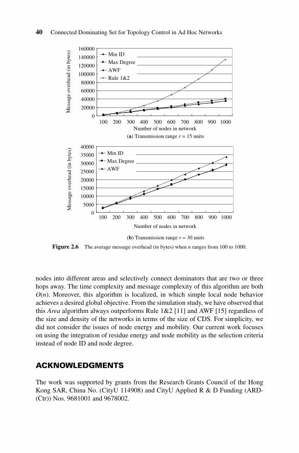
Figure 2.6(a) and (b) relates the message overhead to the number of nodes inthe network (ranging from 100 to 1000 with an increment step of 100) when thetransmission range r is 15 and 30 units, respectively. In both cases, the y-axis denotesthe average number of bytes of messages transmitted by the nodes. Among thesealgorithms, Rule 1&2 consumes the most number of bytes of messages because inthis algorithm each node needs to exchange its one-hop neighbor information with itsone-hop neighbors. When n = 1000 and r = 15, this kind of information exchangeaccounts for about 96% of the total message overhead and demands significant timeand energy consumption. AWF, Min ID, and Max Degree show similar performance
2.6 Conclusion and Future Work 39
0
10
20
30
40
50
60
70
80
100 200 300 400 500 600 700 800 900 1000
Number of nodes in the network
Num
ber
of tw
o-ho
pco
nnec
tors
in th
e C
DS Min ID
Max Degree
AWF
(a) Transmission range r = 15 units
0
4
8
12
16
20
100 200 300 400 500 600 700 800 900 1000
Number of nodes in the network
Num
ber
of tw
o-ho
pco
nnec
tors
in th
e C
DS Min ID
Max Degree
AWF
(b) Transmission range r = 30 units
Figure 2.5 The number of nodes in CDS when r is 30 units.
because in these algorithms each node requires only the knowledge of its one-hopneighbors and a constant number of two-hop and three-hop neighbors. Compared toAWF, Min ID and Max Degree introduce slightly more message overhead in sparsenetworks because one extra item, area ID, is associated with each node in the messageexchange. When n = 1000 and r = 30, the number of bytes of messages consumedby Rule 1&2 is 439,808, nearly 13 times more than that of the other three. To showthe difference between AWF, Min ID, and Max Degree clearly, in Figure 2.6(b) weomit the curve of Rule 1&2.
2.6 CONCLUSION AND FUTURE WORK
In this chapter, we proposed a novel distributed algorithm for connected dominatingset formation in wireless ad hoc networks. In this Area algorithm, we partition the
40 Connected Dominating Set for Topology Control in Ad Hoc Networks
0
20000
40000
60000
80000
100000
120000
140000
160000
100 200 300 400 500 600 700 800 900 1000Number of nodes in network
Mes
sage
ove
rhea
d (i
n by
tes) Min ID
Max Degree
AWF
Rule 1&2
(a) Transmission range r = 15 units
0
5000
10000
15000
20000
25000
30000
35000
40000
100 200 300 400 500 600 700 800 900 1000
Number of nodes in network
Mes
sage
ove
rhea
d (i
n by
tes)
Min ID
Max Degree
AWF
(b) Transmission range r = 30 units
Figure 2.6 The average message overhead (in bytes) when n ranges from 100 to 1000.
nodes into different areas and selectively connect dominators that are two or threehops away. The time complexity and message complexity of this algorithm are bothO(n). Moreover, this algorithm is localized, in which simple local node behaviorachieves a desired global objective. From the simulation study, we have observed thatthis Area algorithm always outperforms Rule 1&2 [11] and AWF [15] regardless ofthe size and density of the networks in terms of the size of CDS. For simplicity, wedid not consider the issues of node energy and mobility. Our current work focuseson using the integration of residue energy and node mobility as the selection criteriainstead of node ID and node degree.
ACKNOWLEDGMENTS
The work was supported by grants from the Research Grants Council of the HongKong SAR, China No. (CityU 114908) and CityU Applied R & D Funding (ARD-(Ctr)) Nos. 9681001 and 9678002.
References 41
REFERENCES
1. B. N. Clark, C. J. Colbourn, and D. S. Johnson. Unit disk graphs. Discrete Math., 86(1–3):165–177,1990.
2. B. Das, R. Sivakumar, and V. Bhargavan. Routing in ad-hoc networks using a spine, Proceedings ofICCCN’1997, pp. 1–20.
3. J. Wu and F. Dai. A generic distributed broadcast scheme in ad hoc wireless networks, Proceedingsof ICDCS’2003, May 2003, pp. 460–468.
4. R. Rajaraman. Topology control and routing in ad hoc networks: a survey, SIGACT News, 33(2):60–73,2002.
5. M. Garey and D. Johnson. Computers and Intractability: A Guide to the Theory of NP-Completeness,Freeman, New York, 1979.
6. S. Basagni, M. Mastrogiovanni, and C. Petrioli. A performance comparison of protocols for clusteringand backbone formation in large scale ad hoc network, Proceedings of MASS’2004, October 2004,pp. 70–79.
7. M. V. Marathe, H. Breu, H. B. Hunt III, S. S. Ravi, and D. J. Rosenkrantz. Simple heuristics for unitdisk graphs. Networks, 25:59–68, 1995.
8. D. Blough, M. Leoncini, G. Resta, and P. Santi. The K-neigh protocol for symmetric topology controlin ad hoc networks. Proceedings of MobiHoc’2003, June 2003, pp. 141–152.
9. W. Wu, H. Du, X. Jia, Y. Li, S. C.-H. Huang, and D.-Z. Du.Maximal independent set and minimumconnected dominating set in unit disk graphs, submitted.
10. S. Guha and S. Khuller. Approximation algorithms for connected dominating sets. Algorithmica,20(4):374–387, 1998.
11. J. Wu and H. Li. On calculating connected dominating set for efficient routing in ad hoc wirelessnetworks, Proceedings of DIALM’1999, pp. 7–14.
12. I. Stojmenovic, S. Seddigh, and J. Zunic. Dominating sets and neighbor elimination based broadcastingalgorithms in wireless networks, IEEE Trans. Parallel Distributed Syst., 13(1):14–25, 2002.
13. R. Sivakumar, P. Sinha, and V. Bharghavan. CEDAR: a core-extraction distributed ad hoc routingalgorithm, IEEE J. Selected Areas Commun., 17(8):1454–1465, 1999.
14. K. M. Alzoubi, P.-J. Wan, and O. Frieder. Distributed heuristics for connected dominating set inwireless ad hoc networks, IEEE ComSoc/KICS J. Commun. Networks, 4(1):22–29, 2002.
15. K. Alzoubi, P.-J. Wan, and O. Frieder. Message-optimal connected dominating sets in mobile ad hocnetworks, Proceedings of MobiHoc’2002, June 2002, pp. 157–164.
16. Y. Li, S. Zhu, M. T. Thai, and D.-Z. Du. Localized construction of connected dominating set in wirelessnetworks, Proceedings of TAWN’2004, June 2004.
17. S. Basagni, Distributed clustering for ad hoc networks, Proceedings of I-SPAN’1999, June 1999,pp. 310–315.
18. R. Wattenhofer, L. Li, P. Bahl, and Y.-M. Wang. Distributed topology control for power efficientoperation in multihop wireless ad hoc networks, Proceedings of IEEE INFOCOM’2001, vol. 3, April2001, pp. 1388–1397.
19. X.-Y. Li, G. Calinescu, and P.-J. Wan. Distributed construction of a planar spanner and routing forad hoc wireless networks. Proceedings of IEEE INFOCOM’2002, vol. 3, June 2002, pp. 1268–1277.
20. R. Ramanathan and R. Rosales-Hain. Topology control of multihop wireless networks using trans-mit power adjustment, Proceedings of IEEE INFOCOM’ 2000, vol. 2, March 2000, pp. 26–30.
21. B. Karp and H. Kung. GPSR: greedy perimeter stateless routing for wireless networks, Proceedingsof MOBICOM’2000, August 2000, pp. 243–254.
22. M. Gerla and J. T.-C. Tsai. Multicluster, mobile, multimedia radio network, Wireless Networks,1(3):255–265, 1995.
23. L. Bao and J. J. Garcia-Luna-Aceves. Topology management in ad hoc networks, Proceedings ofMobiHoc’2003, June 2003, pp. 129–140.
42 Connected Dominating Set for Topology Control in Ad Hoc Networks
24. Y. Wang, W. Wang, and X.-Y. Li, Distributed low-cost backbone formation for wireless ad hocnetworks, Proceedings of MobiHoc’2005, May 2005, pp. 2–13.
25. Z. Gaspar and T. Tarnai. Upper bound of density for packing of equal circles in special domains inthe plane, Periodica Polytech. Ser. CIV. Eng., 44(1):13–32, 2000.
26. E. L. Lloyd, R. Liu, M. V. Marathe, R. Ramanathan, and S. S. Ravi. Algorithmic aspects of topol-ogy control problems for ad hoc networks, Proceedings of MobiHoc’2002, June 2002, pp. 123–134.
27. D. J. Baker, A. Ephremides, and J. A. Flynn. The design and simulation of a mobile radio networkwith distributed control. IEEE J. Selected Areas Commun., 2(1):226–237, 1984.
28. W. R. Heinzelman, A. Chandrakasan, and H. Balakrishnan. Energy efficient communication protocolfor wireless microsensor networks, Proceedings of HICSS’2000, January 2000, pp. 3005–3014.
29. A. Vahdat and D. Becker. Epidemic routing for partially connected ad hoc networks, Technical ReportCS-200006, Duke University, April 2000.
30. W. R. Zhao, M. Ammar, and E. Zegura. A message ferrying approach for data delivery in sparsemobile ad hoc networks, Proceedings of MOBIHOC’2004, May 2004, pp. 187–198.