Modality and Databases Melvin Fitting Dept. Mathematics and Computer Science Lehman College (CUNY), Bronx, NY 10468 e-mail: fi[email protected]web page: comet.lehman.cuny.edu/fitting Abstract. Two things are done in this paper. First, a modal logic in which one can quantify over both objects and concepts is presented; a semantics and a tableau system are given. It is a natural modal logic, ex- tending standard versions, and capable of addressing several well-known philosophical difficulties successfully. Second, this modal logic is used to introduce a rather different way of looking at relational databases. The idea is to treat records as possible worlds, record entries as objects, and attributes as concepts, in the modal sense. This makes possible an in- tuitively satisfactory relational database theory. It can be extended, by the introduction of higher types, to deal with multiple-valued attributes and more complex things, though this is further than we take it here. 1 Introduction A few years ago my colleague, Richard Mendelsohn, and I finished work on our book, “First-Order Modal Logic,” [2]. In it, non-rigidity was given an extensive examination, and formal treatments of definite descriptions, designation, exis- tence, and other issues were developed. I next attempted an extension to higher- order modal logic. After several false starts (or rather, unsatisfactory finishes) this was done, and a book-length manuscript is on my web page inviting com- ments, [1]. Carrying out this extension, in turn, led me to rethink the first-order case. There were two consequences. First, I came to realize that the approach in our book could be extended, without leaving the first-order level, to produce a quite interesting logic with a natural semantics and a tableau proof procedure. And second, I realized that this modal logic provided a natural alternative set- ting for relational databases, which are usually treated using first-order classical logic. In this paper I want to sketch both the modal logic and its application to databases. In a full treatment of first-order modal logic, one must be able to discourse about two kinds of things: individual objects and individual concepts. “George Washington” and “Millard Fillmore” denote individual objects, while “the Pres- ident of the United States” denotes an individual concept, which in turn denotes various individuals at different times. Or again, at the time I am writing this the year is 2000. This particular year is an individual object. “The current year” is an individual concept, and will not always denote 2000. In [2] we had quan- tifiers ranging over individual objects, and constant symbols with values that
Transcript
Modality and Databases
Melvin Fitting
Dept. Mathematics and Computer ScienceLehman College (CUNY), Bronx, NY 10468
Abstract. Two things are done in this paper. First, a modal logic inwhich one can quantify over both objects and concepts is presented; asemantics and a tableau system are given. It is a natural modal logic, ex-tending standard versions, and capable of addressing several well-knownphilosophical difficulties successfully. Second, this modal logic is used tointroduce a rather different way of looking at relational databases. Theidea is to treat records as possible worlds, record entries as objects, andattributes as concepts, in the modal sense. This makes possible an in-tuitively satisfactory relational database theory. It can be extended, bythe introduction of higher types, to deal with multiple-valued attributesand more complex things, though this is further than we take it here.
1 Introduction
A few years ago my colleague, Richard Mendelsohn, and I finished work on ourbook, “First-Order Modal Logic,” [2]. In it, non-rigidity was given an extensiveexamination, and formal treatments of definite descriptions, designation, exis-tence, and other issues were developed. I next attempted an extension to higher-order modal logic. After several false starts (or rather, unsatisfactory finishes)this was done, and a book-length manuscript is on my web page inviting com-ments, [1]. Carrying out this extension, in turn, led me to rethink the first-ordercase. There were two consequences. First, I came to realize that the approach inour book could be extended, without leaving the first-order level, to produce aquite interesting logic with a natural semantics and a tableau proof procedure.And second, I realized that this modal logic provided a natural alternative set-ting for relational databases, which are usually treated using first-order classicallogic. In this paper I want to sketch both the modal logic and its application todatabases.
In a full treatment of first-order modal logic, one must be able to discourseabout two kinds of things: individual objects and individual concepts. “GeorgeWashington” and “Millard Fillmore” denote individual objects, while “the Pres-ident of the United States” denotes an individual concept, which in turn denotesvarious individuals at different times. Or again, at the time I am writing thisthe year is 2000. This particular year is an individual object. “The current year”is an individual concept, and will not always denote 2000. In [2] we had quan-tifiers ranging over individual objects, and constant symbols with values that
2 Melvin Fitting
were individual concepts. That was a good combination to elucidate a numberof well-known philosophical problems, but it is not a full picture. In this paperthe formal system presented will have quantifiers over individual objects, andalso a second kind of quantifier ranging over individual concepts. Likewise therewill be two kinds of constant symbols. The system of [2] can be embedded in thepresent one. (Of course this is only approximate. In our book we had functionsymbols, and we do not have them here. There are other differences as well, butthe embedability claim is essentially correct.) I’ll begin with a presentation ofthe logic, and then consider its applications to databases.
In a sense, using the modal logic of this paper to supply a semantics for rela-tional databases does not give us anything new. We are able to treat things that,previously, had been treated using classical first-order logic. The modal point ofview is substantially different, and hence interesting, but does not expand ourconcept of relational database. The real significance lies in what comes next,just after the conclusion of this paper. The modal logic presented here is thefirst-order fragment of a higher-order modal logic, with both extensional and in-tensional objects at each level. When such a logic is applied to database theory,we get a natural setting within which to model multiple-valued relations, rela-tions having a field whose values are sets of attributes, and more complex thingsyet. Think of the present paper, then, as providing a different point of view onwhat is generally understood, and as signaling the approach of an extension,which can be glimpsed down the road.
2 Syntax
The syntax of this version of first-order modal logic is a little more complex thanusual, and so some care must be taken in its presentation.
There are infinitely many variables and constants, in each of two categories:individual objects and individual concepts. I’ll use lowercase Latin letters x, y,z as object variables, and lowercase Greek letters α, β, γ as concept variables.(Based on the notion that the ancient Greeks were the theoreticians, while theRomans were the engineers.) The Greek letter %, with or without subscripts,represents a variable of either kind. For constants, I’ll use lowercase Latin letterssuch as a, b, c for both kinds, and leave it to context to sort things out.
Definition 1 (Term). A constant symbol or a variable is a term. It is an ob-ject term if it is an individual object variable or constant symbol. Similarly forconcept terms.
If t is a concept term, ↓t is an object term. It is called a relativized term.
The idea is, if t is a concept term, ↓t is intended to designate the objectdenoted by t, in a particular context. Sometimes I’ll refer to ↓ as the evaluate atoperator.
Since there are two kinds of variables and constants, assigning an arity torelation symbols is not sufficient. By a type I mean a finite sequence of o’s and c’s,such as 〈c, o, c〉. Think of an o as marking an object position and a c as marking
Modality and Databases 3
a concept position. There are infinitely many relation symbols of each type. Inparticular there is an equality symbol, =, of type 〈o, o〉. That is, equality is arelation on individual objects. One could also introduce a notion of equality forindividual concepts, but it will not be needed here. I allow the empty sequence〈〉 as a type. It corresponds to what are sometimes called propositional letters,taking no arguments.
Definition 2 (Formula). The set of formulas, and their free variables, is de-fined as follows.
1. If P is a relation symbol of type 〈〉, it is an atomic formula, and has no freevariables.
2. Suppose R is a relation symbol of type 〈n1, n2, . . . , nk〉 and t1, t2, . . . , tk isa sequence of terms such that ti is an individual object term if ni = o andis an individual concept term if ni = c. Then R(t1, t2, . . . , tk) is an atomicformula. Its free variables are the variable occurrences that appear in it.
3. if X is a formula, so are ¬X, 2X, and 3X. Free variable occurrences arethose of X.
4. If X and Y are formulas, so are (X∧Y ), (X∨Y ), and (X ⊃ Y ). Free variableoccurrences are those of X together with those of Y .
5. If X is a formula and % is a variable (of either kind), (∀%)X and (∃%)X areformulas. Free variable occurrences are those of X, except for occurrences of%.
6. If X is a formula, % is a variable (again of either kind), and t is a term of thesame kind as %, 〈λ%.X〉(t) is a formula. Free variable occurrences are thoseof X, except for occurrences of %, together with those of t.
As usual, parentheses will be omitted from formulas to improve readability.Also = (x, y) will be written as x = y. And finally, a formula like
〈λ%1.〈λ%2.〈λ%3.X〉(t3)〉(t2)〉(t1)
will be abbreviated by the simpler expression
〈λ%1, %2, %3.X〉(t1, t2, t3)
and similarly for other formulas involving iterated abstractions.
3 Semantics
I will only formulate an S5 logic—the ideas carry over directly to other logics,but S5 is simplest, the ideas are clearest when stated for it, and it is all that isactually needed for databases.
Frames essentially disappear, since we are dealing with S5. A model has aset of possible worlds, but we can take every world to be accessible from everyother, and so no explicit accessibility relation is needed.
4 Melvin Fitting
The usual constant/varying domain dichotomy is easily ignored. For first-order modal logics generally, a constant domain semantics can simulate a varyingdomain version, through the use of an explicit existence predicate and the rela-tivization of quantifiers to it. Here I’ll take object domains to be constant—notworld dependent—which makes things much simpler.
Since the language has two kinds of terms, we can expect models to havetwo domains—two sorts, in other words. There will be a domain of individualobjects, and a domain of individual concepts. Concepts will be functions, frompossible worlds to individual objects. It is not reasonable, or desirable, to insistthat all such functions be present. After all, if there are countably many possibleworlds, there would be a continuum of such concept functions even if the set ofindividual objects is finite, and this probably cannot be captured by a proofprocedure. But anyway, the notion of an individual concept presupposes a kindof coherency for that individual concept—not all functions would be acceptableintuitively. I simply take the notion of individual concept as basic; I do not tryto analyize any coherency condition. It is allowed that some, not necessarily all,functions can serve as individual concepts.
Definition 3 (Model). A model is a structure M = 〈G,Do,Dc, I〉, where:
1. G is a non-empty set, of possible worlds;2. Do is a non-empty set, of individual objects;3. Dc is a non-empty set of functions from G to Do, called individual concepts;4. I is a mapping that assigns:
(a) to each individual object constant symbol some member of Do;(b) to each individual concept constant symbol some member of Dc;(c) to each relation symbol of type 〈〉 a mapping from G to {false, true};(d) to each relation symbol of type 〈n1, n2, . . . , nk〉 a mapping from G to
the power set of Dn1 ×Dn2 × · · · × Dnk . It is required that I(=) be theconstant mapping that is identically the equality relation on Do.
Some preliminary machinery is needed before truth in a model can be char-acterized.
Definition 4 (Valuation). A valuation v in a model M is a mapping thatassigns to each individual object variable some member of Do, and to each indi-vidual concept variable some member of Dc.
Definition 5 (Value At). Let M = 〈G,Do,Dc, I〉 be a model, and v be avaluation in it. A mapping (v ∗ I) is defined, assigning a meaning to each term,at each possible world. Let Γ ∈ G.
1. If % is a variable, (v ∗ I)(%, Γ ) = v(%).2. If c is a constant symbol, (v ∗ I)(c, Γ ) = I(c).3. If ↓t is a relativized term, (v ∗ I)(↓t, Γ ) = (v ∗ I)(t)(Γ ).
Modality and Databases 5
Item 3 is especially significant. If ↓t is a relativized term, t must be a constantor variable of concept type, and so (v ∗ I)(t) has been defined for it in parts 1and 2, and is a function from worlds to objects. Thus (v ∗ I)(t)(Γ ) is a memberof Do.
Now the main notion, which is symbolized byM, Γ °v Φ, and is read: formulaΦ is true in modelM, at possible world Γ , with respect to valuation v. To makereading easier, the following special notation is used. Let %1, . . . , %k be variablesof any type, and let d1, . . . , dk be members of Do ∪ Dc, with di ∈ Do if thevariable %i is of object type, and di ∈ Dc if %i is of concept type. Then
M, Γ °v Φ[%1/d1, . . . , %k/dk]
abbreviates: M, Γ °v′ Φ where v′ is the valuation that is like v on all variablesexcept %1, . . . , %k, and v′(%1) = d1, . . . , v′(%k) = dk.
Here is the central definition. For simplicity, take ∨, ⊃, ∃, and 3 as definedsymbols, in the usual way.
Definition 6 (Truth in a Model). Let M = 〈G,Do,Dc, I〉 be a model, andv be a valuation in it.
1. If P is of type 〈〉, M, Γ °v P iff I(P )(Γ ) = true.2. If R(t1, . . . , tk) is atomic, M, Γ °v R(t1, . . . , tk) iff〈(v ∗ I)(t1, Γ ), . . . , (v ∗ I)(tk, Γ )〉 ∈ I(R)(Γ ).
3. M, Γ °v ¬Φ iff M, Γ 6°v Φ.4. M, Γ °v Φ ∧ Ψ iff M, Γ °v Φ and M, Γ °v Ψ .5. M, Γ °v (∀x)Φ iff M, Γ °v Φ[x/d] for all d ∈ Do.6. M, Γ °v (∀α)Φ iff M, Γ °v Φ[α/d] for all d ∈ Dc.7. M, Γ °v 2Φ iff M, ∆ °v Φ for all ∆ ∈ G.8. M, Γ °v 〈λ%.Φ〉(t) if M, Γ °v Φ[%/d], where d = (v ∗ I)(t, Γ ).
Definition 7 (Validity). A closed formula X is valid in a model if it is trueat every world of it.
A notion of consequence is a little more complicated because, in modal set-tings, it essentially breaks in two. These are sometimes called local and globalconsequence notions. For a set S of formulas, do we want X to be true at everyworld at which members of S are true (local consequence), or do we want X tobe valid in every model in which members of S are valid (global consequence).These have quite different flavors. Fortunately, for S5, the situation is somewhatsimpler than it is for other modal logics since, to say X is valid in a model isjust to say 2X is true at some world of it. So, if we have a notion of local con-sequence, we can define a corresponding global consequence notion simply byintroducing necessity symbols throughout. So, local consequence is all we needhere.
Definition 8 (Consequence). A closed formula X is a consequence of a set Sof closed formulas if, in every model, X is true at each world at which all themembers of S are true.
6 Melvin Fitting
4 Rigidity
An individual concept term t can vary from world to world in what it designates.Call t rigid in a model if it is constant in that model, designating the same objectat each world. This is a notion that plays an important role in philosophy. Forinstance Kripke [3], among others, asserts that names are rigid designators. Thenotion of rigidity can be captured by a formula. Assume c is an individual conceptconstant symbol in the following.
〈λx.2(x =↓c)〉(↓c) (1)
It is quite straightforward to show that (1) is valid in a model if and only if theinterpretation of c is rigid in that model. In [2] this, in turn, was shown to beequivalent to the vanishing of the de re/de dicto distinction, though this will notbe needed here.
One can also speak of relativized notions of rigidity. Let us say the interpre-tation of c is rigid on a particular subset G0 of the collection G of possible worldsof a model provided it designates the same object throughout G0. And let us sayc is rigid relative to d in a model provided the interpretation of c is rigid on anysubset of worlds on which the interpretation of d is rigid. (Of course, this notionapplies to individual concept terms that are variables as well. I’m using constantsymbols just as a matter of convenience.) The notion of c being rigid relative tod is captured by formula (2).
〈λx, y.2[x =↓d ⊃ y =↓c]〉(↓d, ↓c) (2)
One can also consider more complicated situations. Formula (3) asserts thatc is rigid relative to the rigidity of d and e jointly.
〈λx, y, z.2[(x =↓d ∧ y =↓e) ⊃ z =↓c]〉(↓d, ↓e, ↓c) (3)
Finally, one can even say that all individual concepts are rigid relative toc. This is done in formula (4). Individual concept quantification is obviouslyessential here.
(∀α)〈λx, y.2[x =↓c ⊃ y =↓α]〉(↓c, ↓α) (4)
5 Databases With a Single Relation
In this section we begin taking a look at relational databases. What we consideris quite basic, and can be found in any textbook on databases—[4] is a goodsource. Relational databases are commonly reasoned about using classical first-order logic. I want to show that modal logic is also a natural tool for this purpose.For now, only a single relation will be considered—this will be extended later.
Modality and Databases 7
The record is the basic unit of a relational database, yet it is not a first-classobject in the sense that it is not something we can get as an answer to a query.We could get a record number, perhaps, but not a record. We will take therecords of a relational database to be the possible worlds of a Kripke model. Inany standard modal language possible worlds, in fact, cannot be directly spokenof. The accessibility relation will be the usual S5 one, though there could becircumstances where something more complex might be appropriate.
Entries that fill fields of a relational database generally can be of several datatypes. To keep things simple, let’s say there is just one data type used for thispurpose. (In examples I’ll use strings.) Looking at this in terms of modal logic,these field entries will be the individual objects of a Kripke model.
Next come the attributes themselves. If the database is one listing familyrelationships, say, and there is an attribute recording “father-of,” it has a valuethat varies from record to record, but in every case that value is what we havetaken to be an individual object. In other words, attributes are simply individualconcepts.
The next question is, what about things like functional dependencies, keys,and so on? Let’s begin with the notion of functional dependency. Say we havea relational database in which there are two attributes, call them c and d, andc is functionally dependent on d. Then, if we are at an arbitrary possible world(record) at which c and d have particular values, at any other world at whichd has the value it has in this one, c must also have the same value it has inthis one. This can be expressed by requiring validity of the following formula, inwhich we assume c and d of the Kripke model also occur as individual conceptconstants of the language, and designate themselves.
〈λx, y.2[x =↓d ⊃ y =↓c]〉(↓d, ↓c)But this is just formula (2), and says c is rigid relative to d. In this case, afunctional dependency can be expressed by a relative rigidity assertion.
More complicated functional dependencies also correspond to relative rigidityformulas. For instance, if c is functionally dependent on {d, e}, this is expressedby (3).
Next, what about the notion of keys? As usually treated, to say an attributec is a key is to say there cannot be two records that agree on the value of c.We cannot quite say that, since records cannot directly be spoken of. What wecan say is that two possible worlds agreeing on the value of c must agree on thevalues of all attributes. More formally, this is expressed by the validity of thefollowing formula.
(∀α)〈λx, y.2[x =↓c ⊃ y =↓α]〉(↓c, ↓α)
Note that this is our earlier formula (4).Now, what does the design of a relation schema look like from the present
modal point of view? We must specify the domain for atomic values of the re-lation schema. Semantically, that amounts to specifying the set Do of a modal
8 Melvin Fitting
model. Proof-theoretically, it amounts to saying what the individual object con-stant symbols of the formal language are. (I’ll generally assume that constantsymbols of the language can also occur in models, and designate themselves.)
Next, we must specify what the attributes for the relation schema are. Thisamounts to specifying the set Dc of a model, or the set of individual conceptconstant symbols of a language.
Finally, we must impose some constraints, such as requiring that some at-tribute or set of attributes be a key, or that various functional dependenciesmust hold. This corresponds to taking appropriate relative rigidity formulas asaxioms.
6 A Simple Example
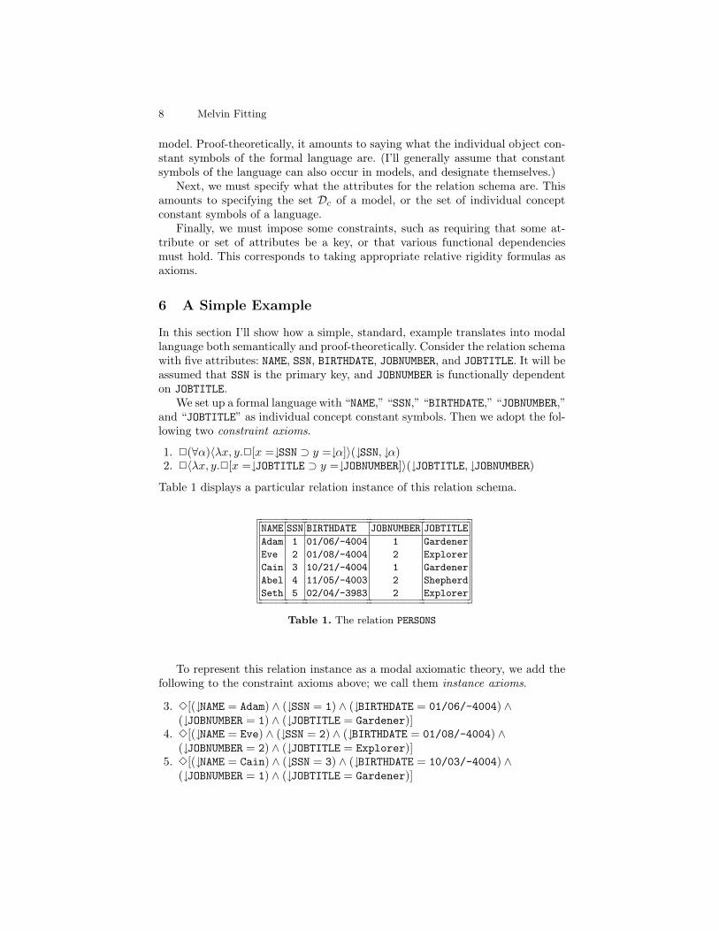
In this section I’ll show how a simple, standard, example translates into modallanguage both semantically and proof-theoretically. Consider the relation schemawith five attributes: NAME, SSN, BIRTHDATE, JOBNUMBER, and JOBTITLE. It will beassumed that SSN is the primary key, and JOBNUMBER is functionally dependenton JOBTITLE.
We set up a formal language with “NAME,” “SSN,” “BIRTHDATE,” “JOBNUMBER,”and “JOBTITLE” as individual concept constant symbols. Then we adopt the fol-lowing two constraint axioms.
1. 2(∀α)〈λx, y.2[x =↓SSN ⊃ y =↓α]〉(↓SSN, ↓α)2. 2〈λx, y.2[x =↓JOBTITLE ⊃ y =↓JOBNUMBER]〉(↓JOBTITLE, ↓JOBNUMBER)
Table 1 displays a particular relation instance of this relation schema.
NAME SSN BIRTHDATE JOBNUMBER JOBTITLE
Adam 1 01/06/-4004 1 Gardener
Eve 2 01/08/-4004 2 Explorer
Cain 3 10/21/-4004 1 Gardener
Abel 4 11/05/-4003 2 Shepherd
Seth 5 02/04/-3983 2 Explorer
Table 1. The relation PERSONS
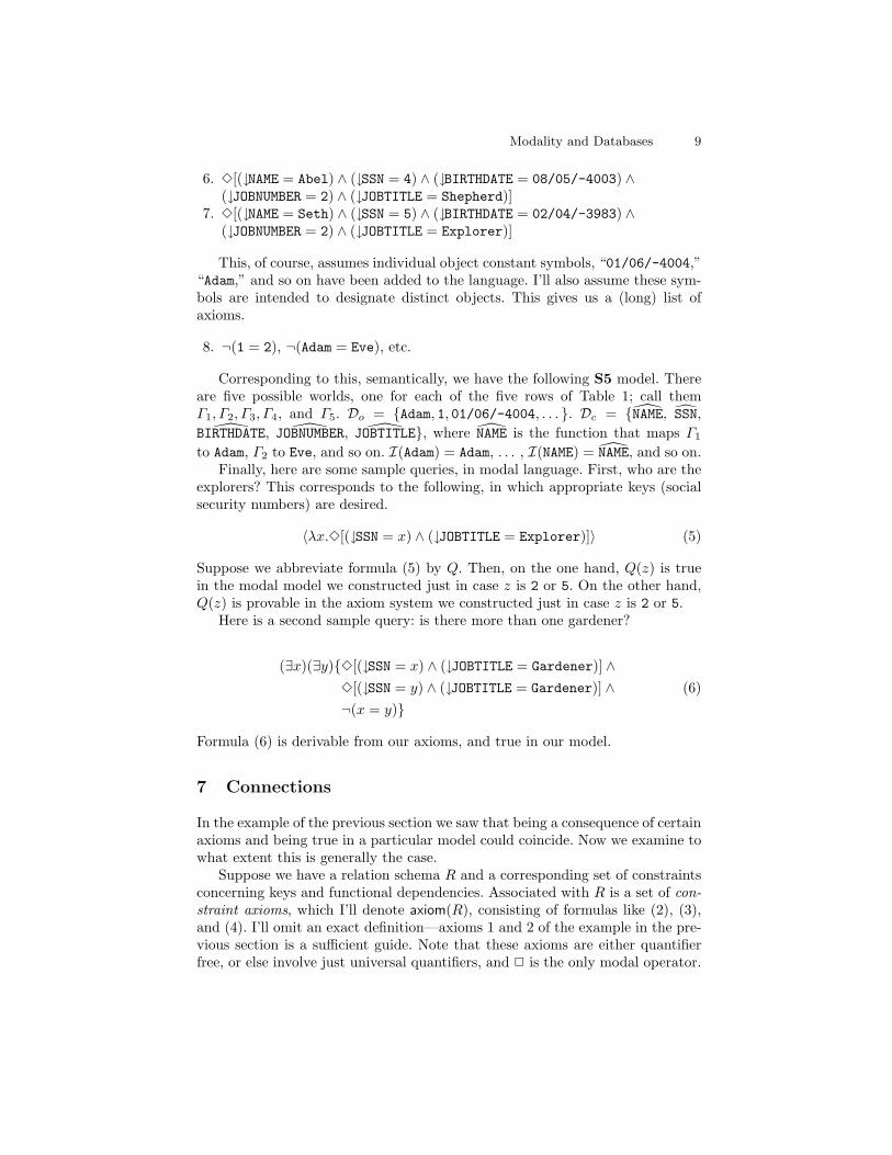
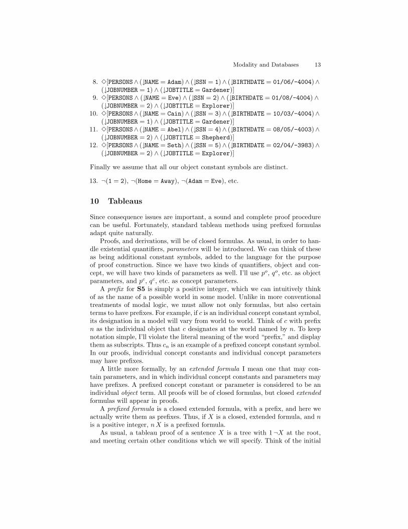
To represent this relation instance as a modal axiomatic theory, we add thefollowing to the constraint axioms above; we call them instance axioms.
This, of course, assumes individual object constant symbols, “01/06/-4004,”“Adam,” and so on have been added to the language. I’ll also assume these sym-bols are intended to designate distinct objects. This gives us a (long) list ofaxioms.
8. ¬(1 = 2), ¬(Adam = Eve), etc.
Corresponding to this, semantically, we have the following S5 model. Thereare five possible worlds, one for each of the five rows of Table 1; call themΓ1, Γ2, Γ3, Γ4, and Γ5. Do = {Adam, 1, 01/06/-4004, . . . }. Dc = {NAME, SSN,BIRTHDATE, JOBNUMBER, JOBTITLE}, where NAME is the function that maps Γ1
to Adam, Γ2 to Eve, and so on. I(Adam) = Adam, . . . , I(NAME) = NAME, and so on.Finally, here are some sample queries, in modal language. First, who are the
explorers? This corresponds to the following, in which appropriate keys (socialsecurity numbers) are desired.
〈λx.3[(↓SSN = x) ∧ (↓JOBTITLE = Explorer)]〉 (5)
Suppose we abbreviate formula (5) by Q. Then, on the one hand, Q(z) is truein the modal model we constructed just in case z is 2 or 5. On the other hand,Q(z) is provable in the axiom system we constructed just in case z is 2 or 5.
Here is a second sample query: is there more than one gardener?
Formula (6) is derivable from our axioms, and true in our model.
7 Connections
In the example of the previous section we saw that being a consequence of certainaxioms and being true in a particular model could coincide. Now we examine towhat extent this is generally the case.
Suppose we have a relation schema R and a corresponding set of constraintsconcerning keys and functional dependencies. Associated with R is a set of con-straint axioms, which I’ll denote axiom(R), consisting of formulas like (2), (3),and (4). I’ll omit an exact definition—axioms 1 and 2 of the example in the pre-vious section is a sufficient guide. Note that these axioms are either quantifierfree, or else involve just universal quantifiers, and 2 is the only modal operator.
10 Melvin Fitting
Next, suppose we have a relation instance r of the relation schema R—aparticular set of tuples. Associated with this is a set of instance axioms, all ofwhich are quantifier free. Again I omit an exact definition, but axioms 3–7 of theprevious section illustrate the notion sufficiently. Finally there are distinctnessaxioms, as in axiom 8 of the previous section. By axiom(r) I mean the collectionof these instance axioms and distinctness axioms, together with the members ofaxiom(R). Clearly, to say r is an instance of R and satisfies the constraints, isjust to say axiom(r) is a consistent set of model axioms.
Next, we want a designated modal model to correspond to relation instancer. Again, the example of the previous section serves as a guide. We want themodel, denote it by model(r), meeting the following conditions. The collectionof possible worlds G is the collection of tuples in r. The domain Do of individualobjects is just the collection of table entries in r. The domain Dc of individualconcepts is the collection of attributes of relation schema R. The interpretationI maps each table entry (as a constant of the modal language) to itself (as amember of Do). And I maps each attribute ATT to the function whose value attuple (possible world) Γ is the entry in the tuple Γ corresponding to ATT. Theonly relation symbol is =, which is interpreted as equality on Do.
Question: what are the connections between axiom(r) and model(r)? I don’tknow the most general answer to this, but here is something that accounts forwhat was seen in the previous section. Note that the queries considered there,formulas (5) and (6), were either quantifier free or involved existential quantifiersof individual object type only. This is significant.
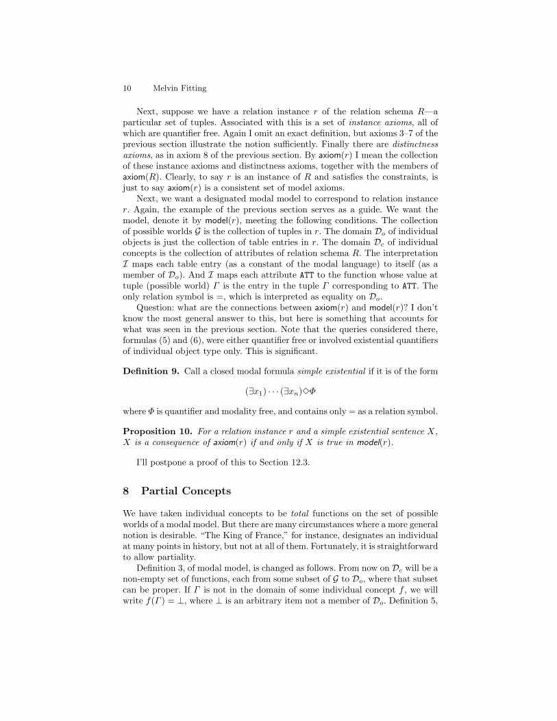
Definition 9. Call a closed modal formula simple existential if it is of the form
(∃x1) · · · (∃xn)3Φ
where Φ is quantifier and modality free, and contains only = as a relation symbol.
Proposition 10. For a relation instance r and a simple existential sentence X,X is a consequence of axiom(r) if and only if X is true in model(r).
I’ll postpone a proof of this to Section 12.3.
8 Partial Concepts
We have taken individual concepts to be total functions on the set of possibleworlds of a modal model. But there are many circumstances where a more generalnotion is desirable. “The King of France,” for instance, designates an individualat many points in history, but not at all of them. Fortunately, it is straightforwardto allow partiality.
Definition 3, of modal model, is changed as follows. From now on Dc will be anon-empty set of functions, each from some subset of G to Do, where that subsetcan be proper. If Γ is not in the domain of some individual concept f , we willwrite f(Γ ) = ⊥, where ⊥ is an arbitrary item not a member of Do. Definition 5,
Modality and Databases 11
value at, can be used with no change in wording, but notice that the scope ofpart 3 has been extended. If ↓t is a relativized term, and Γ is not in the domainof (v ∗ I)(t), then (v ∗ I)(↓t, Γ ) = (v ∗ I)(t)(Γ ) = ⊥.
Now Definition 6, truth in a model, must also be modified. I’ll follow thepretty obvious general principle that one cannot ascribe properties to what isdesignated by a non-designating term. In the Definition, item 2 is changed toread as follows.
2. If R(t1, . . . , tk) is atomic,(a) if any of (v∗I)(t1, Γ ), . . . , (v∗I)(tk, Γ ) is ⊥ thenM, Γ 6°v R(t1, . . . , tk);(b) otherwise M, Γ °v R(t1, . . . , tk) iff 〈(v ∗ I)(t1, Γ ), . . . , (v ∗ I)(tk, Γ )〉 ∈I(R)(Γ ).
Also item 8 must be changed.
8. For an abstract 〈λ%.Φ〉(t),(a) if (v ∗ I)(t, Γ ) = ⊥, M, Γ 6°v 〈λ%.Φ〉(t);(b) otherwiseM, Γ °v 〈λ%.Φ〉(t) ifM, Γ °v Φ[%/d], where d = (v ∗ I)(t, Γ ).
Notice that, with the definitions modified in this way, ↓t =↓t is true at aworld of a model if and only if the term t “designates” at that world. Thismakes possible the following piece of machinery.
Definition 11 (Designation Formula). D abbreviates the abstract 〈λα. ↓α =↓α〉.
Clearly M, Γ °v D(t) iff (v ∗ I)(t, Γ ) 6= ⊥, where M = 〈G,Do,Dc, I〉. Thus Dreally does express the notion of designation.
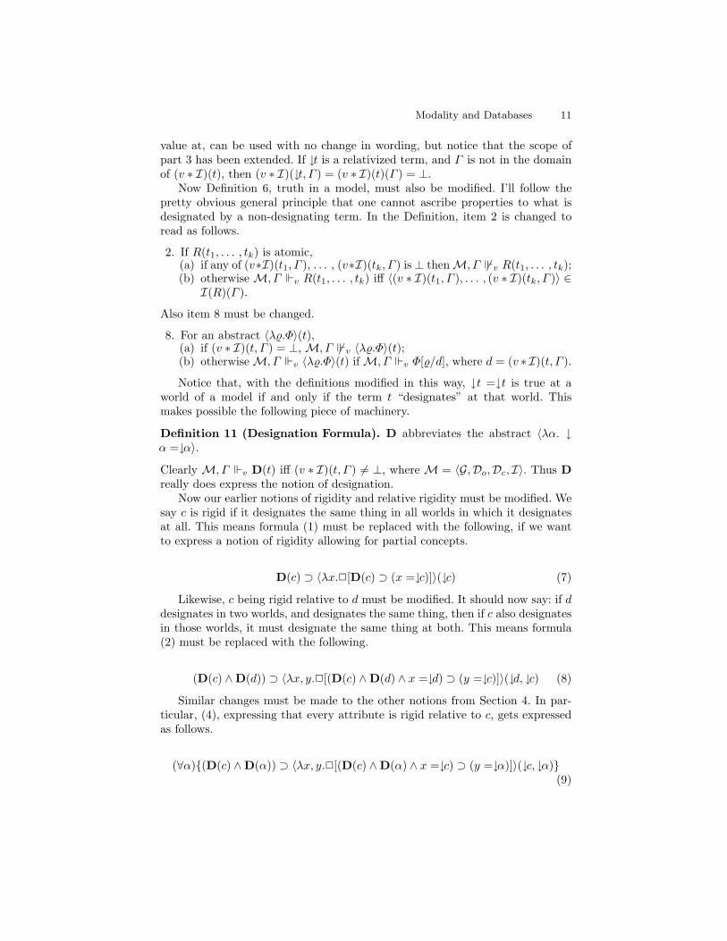
Now our earlier notions of rigidity and relative rigidity must be modified. Wesay c is rigid if it designates the same thing in all worlds in which it designatesat all. This means formula (1) must be replaced with the following, if we wantto express a notion of rigidity allowing for partial concepts.
D(c) ⊃ 〈λx.2[D(c) ⊃ (x =↓c)]〉(↓c) (7)
Likewise, c being rigid relative to d must be modified. It should now say: if ddesignates in two worlds, and designates the same thing, then if c also designatesin those worlds, it must designate the same thing at both. This means formula(2) must be replaced with the following.
Similar changes must be made to the other notions from Section 4. In par-ticular, (4), expressing that every attribute is rigid relative to c, gets expressedas follows.
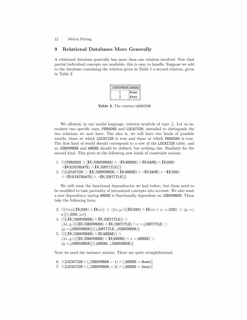
A relational database generally has more than one relation involved. Now thatpartial individual concepts are available, this is easy to handle. Suppose we addto the database containing the relation given in Table 1 a second relation, givenin Table 2.
JOBNUMBER WHERE
1 Home
2 Away
Table 2. The relation LOCATION
We allowed, in our modal language, relation symbols of type 〈〉. Let us in-troduce two specific ones, PERSONS and LOCATION, intended to distinguish thetwo relations we now have. The idea is, we will have two kinds of possibleworlds, those at which LOCATION is true and those at which PERSONS is true.The first kind of world should correspond to a row of the LOCATION table, andso JOBNUMBER and WHERE should be defined, but nothing else. Similarly for thesecond kind. This gives us the following new kinds of constraint axioms.
We still want the functional dependencies we had before, but these need tobe modified to take partiality of intensional concepts into account. We also wanta new dependency saying WHERE is functionally dependent on JOBNUMBER. Thesetake the following form.
Finally we assume that all our object constant symbols are distinct.
13. ¬(1 = 2), ¬(Home = Away), ¬(Adam = Eve), etc.
10 Tableaus
Since consequence issues are important, a sound and complete proof procedurecan be useful. Fortunately, standard tableau methods using prefixed formulasadapt quite naturally.
Proofs, and derivations, will be of closed formulas. As usual, in order to han-dle existential quantifiers, parameters will be introduced. We can think of theseas being additional constant symbols, added to the language for the purposeof proof construction. Since we have two kinds of quantifiers, object and con-cept, we will have two kinds of parameters as well. I’ll use po, qo, etc. as objectparameters, and pc, qc, etc. as concept parameters.
A prefix for S5 is simply a positive integer, which we can intuitively thinkof as the name of a possible world in some model. Unlike in more conventionaltreatments of modal logic, we must allow not only formulas, but also certainterms to have prefixes. For example, if c is an individual concept constant symbol,its designation in a model will vary from world to world. Think of c with prefixn as the individual object that c designates at the world named by n. To keepnotation simple, I’ll violate the literal meaning of the word “prefix,” and displaythem as subscripts. Thus cn is an example of a prefixed concept constant symbol.In our proofs, individual concept constants and individual concept parametersmay have prefixes.
A little more formally, by an extended formula I mean one that may con-tain parameters, and in which individual concept constants and parameters mayhave prefixes. A prefixed concept constant or parameter is considered to be anindividual object term. All proofs will be of closed formulas, but closed extendedformulas will appear in proofs.
A prefixed formula is a closed extended formula, with a prefix, and here weactually write them as prefixes. Thus, if X is a closed, extended formula, and nis a positive integer, nX is a prefixed formula.
As usual, a tableau proof of a sentence X is a tree with 1¬X at the root,and meeting certain other conditions which we will specify. Think of the initial
14 Melvin Fitting
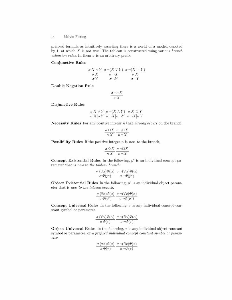
prefixed formula as intuitively asserting there is a world of a model, denotedby 1, at which X is not true. The tableau is constructed using various branchextension rules. In them σ is an arbitrary prefix.
Conjunctive Rules
σX ∧ YσXσ Y
σ ¬(X ∨ Y )σ ¬Xσ ¬Y
σ ¬(X ⊃ Y )σXσ ¬Y
Double Negation Rule
σ ¬¬XσX
Disjunctive Rules
σX ∨ YσX σ Y
σ ¬(X ∧ Y )σ ¬X σ ¬Y
σX ⊃ Yσ ¬X σ Y
Necessity Rules For any positive integer n that already occurs on the branch,
σ2XnX
σ ¬3Xn¬X
Possibility Rules If the positive integer n is new to the branch,
σ3XnX
σ ¬2Xn¬X
Concept Existential Rules In the following, pc is an individual concept pa-rameter that is new to the tableau branch.
σ (∃α)Φ(α)σ Φ(pc)
σ ¬(∀α)Φ(α)σ ¬Φ(pc)
Object Existential Rules In the following, po is an individual object param-eter that is new to the tableau branch.
σ (∃x)Φ(x)σ Φ(po)
σ ¬(∀x)Φ(x)σ ¬Φ(po)
Concept Universal Rules In the following, τ is any individual concept con-stant symbol or parameter.
σ (∀α)Φ(α)σ Φ(τ)
σ ¬(∃α)Φ(α)σ ¬Φ(τ)
Object Universal Rules In the following, τ is any individual object constantsymbol or parameter, or a prefixed individual concept constant symbol or param-eter.
σ (∀x)Φ(x)σ Φ(τ)
σ ¬(∃x)Φ(x)σ ¬Φ(τ)
Modality and Databases 15
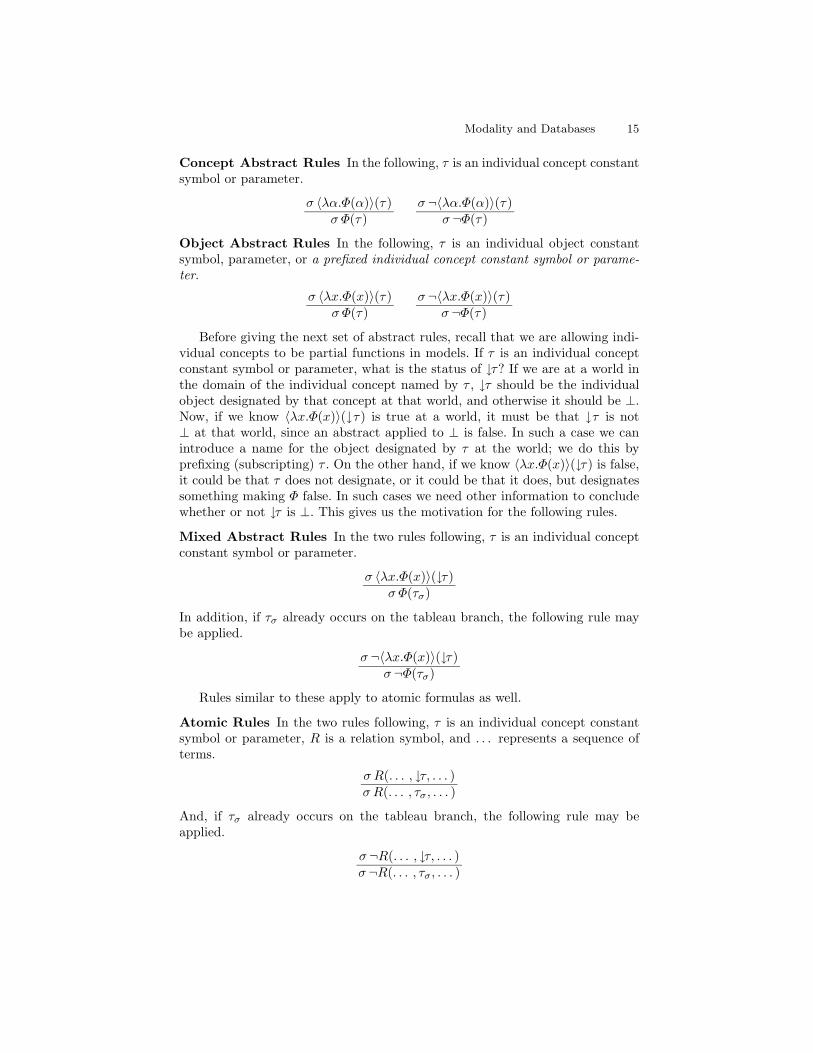
Concept Abstract Rules In the following, τ is an individual concept constantsymbol or parameter.
σ 〈λα.Φ(α)〉(τ)σ Φ(τ)
σ ¬〈λα.Φ(α)〉(τ)σ ¬Φ(τ)
Object Abstract Rules In the following, τ is an individual object constantsymbol, parameter, or a prefixed individual concept constant symbol or parame-ter.
σ 〈λx.Φ(x)〉(τ)σ Φ(τ)
σ ¬〈λx.Φ(x)〉(τ)σ ¬Φ(τ)
Before giving the next set of abstract rules, recall that we are allowing indi-vidual concepts to be partial functions in models. If τ is an individual conceptconstant symbol or parameter, what is the status of ↓τ? If we are at a world inthe domain of the individual concept named by τ , ↓τ should be the individualobject designated by that concept at that world, and otherwise it should be ⊥.Now, if we know 〈λx.Φ(x)〉(↓τ) is true at a world, it must be that ↓τ is not⊥ at that world, since an abstract applied to ⊥ is false. In such a case we canintroduce a name for the object designated by τ at the world; we do this byprefixing (subscripting) τ . On the other hand, if we know 〈λx.Φ(x)〉(↓τ) is false,it could be that τ does not designate, or it could be that it does, but designatessomething making Φ false. In such cases we need other information to concludewhether or not ↓τ is ⊥. This gives us the motivation for the following rules.
Mixed Abstract Rules In the two rules following, τ is an individual conceptconstant symbol or parameter.
σ 〈λx.Φ(x)〉(↓τ)σ Φ(τσ)
In addition, if τσ already occurs on the tableau branch, the following rule maybe applied.
σ ¬〈λx.Φ(x)〉(↓τ)σ ¬Φ(τσ)
Rules similar to these apply to atomic formulas as well.
Atomic Rules In the two rules following, τ is an individual concept constantsymbol or parameter, R is a relation symbol, and . . . represents a sequence ofterms.
σ R(. . . , ↓τ, . . . )σ R(. . . , τσ, . . . )
And, if τσ already occurs on the tableau branch, the following rule may beapplied.
σ ¬R(. . . , ↓τ, . . . )σ ¬R(. . . , τσ, . . . )
16 Melvin Fitting
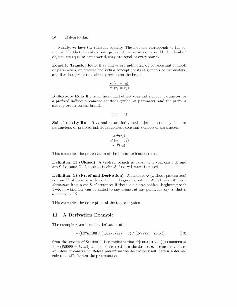
Finally, we have the rules for equality. The first one corresponds to the se-mantic fact that equality is interpreted the same at every world; if individualobjects are equal at some world, they are equal at every world.
Equality Transfer Rule If τ1 and τ2 are individual object constant symbolsor parameters, or prefixed individual concept constant symbols or parameters,and if σ′ is a prefix that already occurs on the branch
σ (τ1 = τ2)σ′ (τ1 = τ2)
Reflexivity Rule If τ is an individual object constant symbol, parameter, ora prefixed individual concept constant symbol or parameter, and the prefix σalready occurs on the branch,
σ (τ = τ)
Substitutivity Rule If τ1 and τ2 are individual object constant symbols orparameters, or prefixed individual concept constant symbols or parameters
σ Φ(τ1)σ′ (τ1 = τ2)σ Φ(τ2)
This concludes the presentation of the branch extension rules.
Definition 12 (Closed). A tableau branch is closed if it contains σX andσ ¬X for some X. A tableau is closed if every branch is closed.
Definition 13 (Proof and Derivation). A sentence Φ (without parameters)is provable if there is a closed tableau beginning with 1¬Φ. Likewise, Φ has aderivation from a set S of sentences if there is a closed tableau beginning with1¬Φ, in which 1X can be added to any branch at any point, for any X that isa member of S.
This concludes the description of the tableau system.
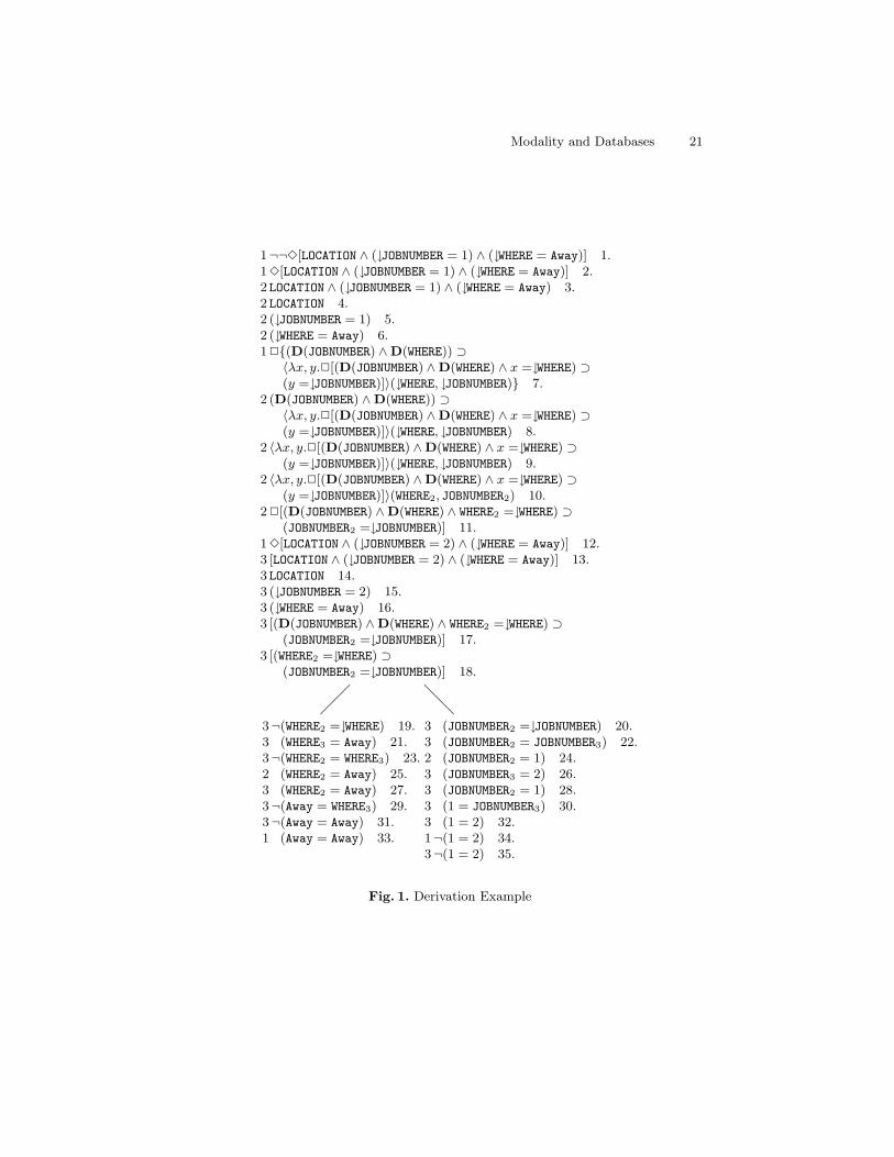
from the axioms of Section 9. It establishes that 3[LOCATION ∧ (↓JOBNUMBER =1) ∧ (↓WHERE = Away)] cannot be inserted into the database, because it violatesan integrity constraint. Before presenting the derivation itself, here is a derivedrule that will shorten the presentation.
Modality and Databases 17
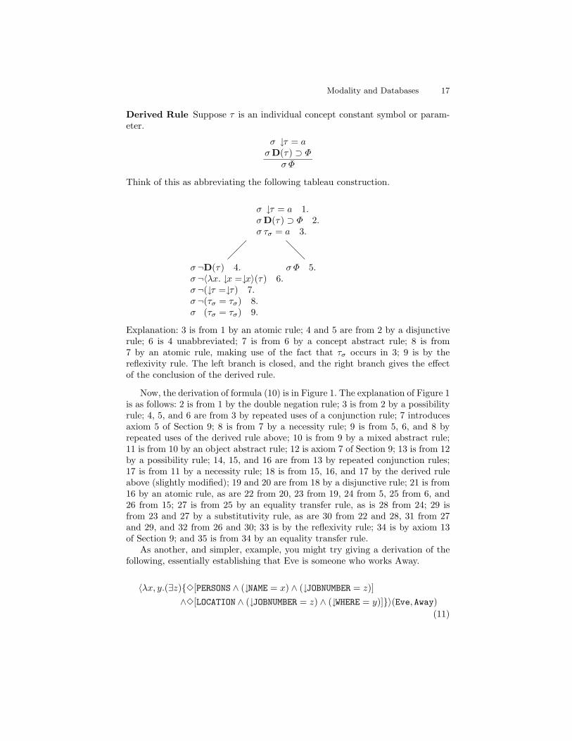
Derived Rule Suppose τ is an individual concept constant symbol or param-eter.
σ ↓τ = aσD(τ) ⊃ Φ
σ Φ
Think of this as abbreviating the following tableau construction.
Explanation: 3 is from 1 by an atomic rule; 4 and 5 are from 2 by a disjunctiverule; 6 is 4 unabbreviated; 7 is from 6 by a concept abstract rule; 8 is from7 by an atomic rule, making use of the fact that τσ occurs in 3; 9 is by thereflexivity rule. The left branch is closed, and the right branch gives the effectof the conclusion of the derived rule.
Now, the derivation of formula (10) is in Figure 1. The explanation of Figure 1is as follows: 2 is from 1 by the double negation rule; 3 is from 2 by a possibilityrule; 4, 5, and 6 are from 3 by repeated uses of a conjunction rule; 7 introducesaxiom 5 of Section 9; 8 is from 7 by a necessity rule; 9 is from 5, 6, and 8 byrepeated uses of the derived rule above; 10 is from 9 by a mixed abstract rule;11 is from 10 by an object abstract rule; 12 is axiom 7 of Section 9; 13 is from 12by a possibility rule; 14, 15, and 16 are from 13 by repeated conjunction rules;17 is from 11 by a necessity rule; 18 is from 15, 16, and 17 by the derived ruleabove (slightly modified); 19 and 20 are from 18 by a disjunctive rule; 21 is from16 by an atomic rule, as are 22 from 20, 23 from 19, 24 from 5, 25 from 6, and26 from 15; 27 is from 25 by an equality transfer rule, as is 28 from 24; 29 isfrom 23 and 27 by a substitutivity rule, as are 30 from 22 and 28, 31 from 27and 29, and 32 from 26 and 30; 33 is by the reflexivity rule; 34 is by axiom 13of Section 9; and 35 is from 34 by an equality transfer rule.
As another, and simpler, example, you might try giving a derivation of thefollowing, essentially establishing that Eve is someone who works Away.
In this section I’ll sketch soundness and completeness arguments for the tableausystem, as well as give a proof for Proposition 10. Nothing is given in muchdetail, because proofs are straightforward adaptations of what are, by now, fairlystandard arguments.
12.1 Soundness
Soundness is by the usual tableau method. One defines a notion of satisfiabilityfor prefixed formulas—a set S is satisfiable if there is a modelM, a mapping massigning to each prefix σ a possible world m(σ) of M, and a formula Φ is trueat world m(σ) ofM whenever σ Φ ∈ S. A tableau is called satisfiable if the set ofprefixed formulas on one of its branches is satisfiable. Then one shows that eachtableau rule preserves tableau satisfiability. This requires a case by case check.
Now, if there is a closed tableau for 1¬X, then X must be valid. For, other-wise, there would be some model in which X was false at some world. It followsthat the set {1¬X} is satisfiable, so we begin with a satisfiable tableau. Thenwe can only get satisfiable tableaus, and since we had a closed tableau for 1¬Xwe have the impossible situation of having a closed, satisfiable tableau.
12.2 Completeness
Suppose X is a sentence that has no tableau proof—it must be shown that Xis not valid. Again the methodology is standard. Also, while the proof sketchbelow is just for tableau provability, and not derivability, the argument extendsdirectly. I’m giving the simpler version, for simplicity.
Begin by constructing a tableau for 1¬X, and do so systematically, in sucha way that all tableau rules are fairly applied. That is, during the tableau con-struction, any rule that could eventually be applied is. There are many suchfair tableau construction procedures—I’ll leave the details to you. The result isa tableau that does not close—say it has an open branch θ (Konig’s lemma isneeded to guarantee such a branch exists, if the tableau construction is infinite).
Now, construct a model as follows.
1. The set G of possible worlds is the set of prefixes that occur on branch θ.2. The domain Do of objects is the set consisting of: all individual object con-
stant symbols of the language, all individual object parameters that occuron θ, and all subscripted (prefixed) individual concept constant symbols andparameters that occur on θ.
3. if f is an individual concept constant symbol, or individual concept param-eter that occurs on θ, a function f is defined as follows. The domain of f isthe set of prefixes σ such that fσ occurs on θ. And if σ is in the domain off then f(σ) = fσ. Note that f maps a subset of G to Do. The domain Dc ofconcepts is the set of all these f .
4. For the interpretation I:
Modality and Databases 19
(a) I assigns to each member of Do itself.(b) I assigns to each f that is an individual concept constant or parameter
(on θ) the function f .(c) I assigns to a relation symbol P of type 〈〉 the mapping from G to{false, true} such that I(P )(σ) = true iff σ P occurs on θ.
(d) To make this clause easier to state, I’ll use the following notation. If fis an object symbol, set f = f . If f is a concept constant or parameter,f has already been defined. Now, I assigns to a relation symbol R oftype 〈n1, n2, . . . , nk〉 a mapping on G such that 〈t1, . . . , tk〉 ∈ I(R)(σ)iff σ R(t1, . . . , tk) occurs on θ.
This completes the definition of a model, call it M. Actually, the equalitysymbol may not be interpreted by equality, but leaving this aside for the moment,one can show by standard methods involving an induction on formula degreethat, for any valuation v:
– If σ Φ occurs on θ then M, σ °v Φ.– If σ ¬Φ occurs on θ then M, σ 6°v Φ.
The valuation v can be arbitrary because free variables do not occur in tableaus.Since 1¬X begins the tableau, it occurs on θ, and hence X is not valid in Msince it is false at world 1.
Finally, one “factors” the modelM using the equivalence relation that is theinterpretation of the equality symbol, turning it into a normal modal model. TheEquality Transfer Rule tells us that the interpretation of the equality symbol willbe the same at every world of M. I’ll leave details to you.
12.3 A Sketch of Proposition 10
Assume r is a relation instance and X a simple existential sentence X. Allmembers axiom(r) are true in model(r), so if X is a consequence of axiom(r),then X will be true in model(r). It is the converse direction that needs work.
Suppose X is not a consequence of axiom(r). Then X does not have a tableauderivation from axiom(r). Suppose we now carry out the steps of the complete-ness argument, from Section 12.2. We begin a tableau for 1¬X, carry out itsconstruction systematically and, since it is a derivation, we introduce membersof axiom(r) onto the branch during the construction. As usual, I’ll omit details.
Members of axiom(r) that are constraint axioms all involve 2 in a positivelocation—they do not involve 3. The sentence X is simple existential, and so¬X contains 3 in a negative location—it behaves like 2. None of these formulas,then, can invoke applications of a possibility rule. Only the instance axioms ofaxiom(r) can do this. So, if there are n members of axiom(r) that are instanceaxioms, an open tableau branch will have exactly n + 1 different prefixes onit: prefix 1 with which we started, and the n additional prefixes introduced bypossibility rule applications to instance axioms.
Now, proceed with the construction of a model, using an open tableau branch,as outlined in Section 12.2. We get a model with n+ 1 worlds, with X is false at
20 Melvin Fitting
world 1, and a world corresponding to each instance axiom. Because of the formof X (only existential quantifiers and a single possibility symbol), since it is falseat world 1, it is also false at every world. If we now consider the submodel inwhich world 1 is dropped, it is not hard to check that truth values of membersof axiom(r) do not change at remaining worlds, nor does the truth value of X.And the resulting model is (isomorphic to) model(r).
13 Conclusion
I want to finish by describing two plausible directions for future work, one havingto do with the modal logic directly, the other with its applications to databases.
The tableau proof procedure given here used parameters and, as such, ismeant for human application. But it should be possible to develop a free-variableversion that can be automated. The S5 modality itself is a kind of quantifier,but it is of a simple nature. Object quantification is essentially classical. Con-cept quantification may create some difficulty—I don’t know. Equality plays afundamental role, but it is a rather simple one. Perhaps what is needed can becaptured efficiently in an automated proof procedure.
The databases considered here were all conventional relational ones. This iswhat the first-order modal language can handle. But one could consider multiple-valued databases, say, in which entries can be sets. Or for a more complicated ex-ample, consider this. Say a record represents a person, and among a person’s at-tributes are these three: FAVORITE BOOK, FAVORITE MOVIE, and MOST IMPORTANT.The first two attributes have the obvious meaning. The MOST IMPORTANT at-tribute records which that person considers most important in evaluating some-one, FAVORITE BOOK or FAVORITE MOVIE. Thus MOST IMPORTANT is an attributewhose value is an attribute. (This example is meant to be easily described, andhence is rather artificial. More realistic examples are not hard to come by.) Themodal logic of this paper is really the first-order fragment of a higher-type sys-tem, presented in full in [1]. If one uses that, one can easily have sets of objects,or attributes, as entries. Indeed, one can consider much more complex thingsyet. Of course the proof procedure also becomes more complex, as one wouldexpect. Whether such things are of use remains to be seen.
References
1. Melvin C. Fitting. Types, Tableaus, and Godel’s God. 2000. Available on my website: comet.lehman.cuny.edu/fitting.
2. Melvin C. Fitting and Richard Mendelsohn. First-Order Modal Logic. Kluwer, 1998.Paperback, 1999.
3. Saul Kripke. Naming and Necessity. Harvard University Press, 1980.4. Jeffrey D. Ullman. Principles of Database and Knowledge-Base Systems, volume 1.