MODE: Mix Driven On-line Resource Demand Estimation

Amir Kalbasi, Diwakar Krishnamurthy

Electrical and Computer Engineering

University of Calgary

Calgary, Canada

Jerry Rolia

Services Research Lab

Hewlett Packard Labs

Palo Alto, CA, USA

Michael Richter

Computer Science

University of Calgary

Calgary, Canada

Abstract— Adaptive performance management solutions often

rely on models that require accurate resource demand measures

that are estimated in an on-line manner. However it is typically

not possible to directly measure resource demands at the

abstraction they are needed, e.g., for a software service within an

application server that is invoked by a URL. For such cases,

linear regression techniques are often used to estimate resource

demands. We evaluate the effectiveness of the Least Squares

(LSQ) and Least Absolute Deviations (LAD) regression

techniques, used extensively by others, as well as Support Vector

Regression (SVR) for the purpose of demand estimation. To the

best of our knowledge SVR has not yet been evaluated for

computer resource demand estimation. We consider the

predictive accuracy of these methods for three different real and

simulated workloads. Our results demonstrate the importance of

tuning the regression parameters of the techniques. We propose

an on-line method named Mix Driven On-line Resource Demand

Estimation (MODE) that automatically and quickly tunes the

regression parameters for LSQ, LAD, and SVR to achieve their

best results. The method is novel in that it relies on pre-defined

workload mixes with known aggregate demand values to support

the tuning exercise. We show that when employed in an on-line

manner, tuning with respect to pre-defined mixes is significantly

more accurate than the traditional approach of using only step by

step data.

Keywords-component; Benchmarking, resource demand

prediction, statistical regression

I. INTRODUCTION

Quantitative performance models are often used to support the adaptive management of applications and systems. They typically require resource demand estimates for model parameters. However, resource demand prediction can be difficult because computer measurement systems do not always offer resource usage measurements at the desired abstraction. For example, total server CPU utilization over some time interval and operating system process CPU utilization over some time interval may be available whereas the utilization of a CPU by a particular software function or transaction is not. Software level monitoring and logging facilities often provide counts for the number of times software functions are invoked and even measures of response times. However relating these to demands is difficult, particularly in distributed and multi-tier environments. In these environments, application servers are often multi-threaded and frequently exploit virtualization technologies and hosts that have multiple CPUs. This paper considers several techniques that can be used to estimate resource demands in such environments.

Regression techniques have been widely used ‎[2] ‎[13] ‎[14] ‎[15] ‎[16] ‎[18] ‎[19] to support demand prediction by estimating per-function demands. The aggregate demand of a new

workload function mix can be estimated as the product of the expected throughput of software functions in the new workload and their corresponding demands as estimated by regression. The accuracy of the aggregate demand estimate depends on the accuracy of the individual per-function demand estimates. If such estimates are poor then the effectiveness of quantitative models and methods that depend on them will suffer.

Previous studies ‎[14] ‎[15] ‎[16] ‎[19] have shown that the accuracy of regression techniques suffer if the per-function demands for a system are not deterministic, which is generally the case for computer systems. Furthermore, many regression techniques suffer from the well-studied problem of multi-collinearity ‎[6] which can lead to unreliable predictions for demands. We applied the machine learning based Support Vector Regression (SVR) method to this same problem to determine whether it does better than standard regression techniques such as Least Squares (LSQ) and Least Absolute Deviations (LAD). Our results show that in some cases it does do better. However it does not always do better and it requires more effort to tune for good results. Our study reveals that each method outperforms the others in certain workload specific circumstances.

Our proposed solution to the demand estimation problem is a technique we call Mix Driven On-line Resource Demand Estimation (MODE) that supports a suite of regression-based demand estimation methods. In on-line demand estimation, recent traces of system activity are used to predict future per-function demands. Such methods exploit temporal correlations in resource demand patterns between successive periods of system activity. Our MODE technique assumes accurate aggregate demand measurements are available for a number of pre-existing workload function mixes. Then as demand estimates are required, these pre-existing measurements are used to automatically tune in an on-line manner each demand estimation technique employed at each step in the on-line prediction process. The use of pre-defined workload mixes for tuning significantly outperforms the traditional approach of tuning regression in a step by step manner using only recent information.

Section 2 describes related work on demand estimation. Our use of LSQ, LAD, and SVR for computer system demand estimation is described in Section 3. Section 4 provides a brief description of MODE. Section 5 describes our experimental setup and study. Section 6 presents the results of the traditional approach of using only step by step data and when using MODE. Section 7 offers summary and concluding remarks.

II. RELATED WORK

Bard and Shatzoff studied the problem of characterizing the resource‎usage‎of‎operating‎system‎functions‎in‎the‎1970’s‎‎[2]. The system under study did not have the ability to measure the resource demands of such functions directly. The execution rates of the functions and their aggregate resource consumption were measurable and were recorded periodically. Each recorded sample served as a window and the windows collected in this manner served as inputs to a regression problem. Bard used the LSQ technique to successfully estimate per-function resource consumption for the study.

Regression techniques have been employed to estimate the resource demands of distributed software systems since the 90’s‎ ‎[4] ‎[15] ‎[16] ‎[24]. Pacifici et al. ‎[13] describe an application of regression for on-line demand estimation that employed LSQ and the aging of measurement traces that contribute to estimates ‎[13]. Many of these studies reported challenges applying the techniques, in particular issues relating to non-deterministic demands and multi-collinearity.

Surprisingly, not many regression-based demand estimation studies have considered in detail the impact of selecting appropriate window sizes, i.e., the time duration of each measurement sample used by regression. Some studies consider a fixed window size when estimating per-function demand using LSQ and LAD ‎[4] ‎[18]. Zhang et al. apply LSQ regression technique to estimate the per-function demands and hence the resource utilizations of a TPC-W system ‎[21]. Their study considered 4 different window sizes and concluded that the larger window sizes are better. Our study shows that the accuracy of demand estimates can be very sensitive to the choice of window size and that this choice is workload dependent. In particular, our results show that accuracies can increase to a point with window size, but may then decrease again.

Recently several studies have investigated alternatives to

regression based approaches. Some techniques employ the use

of queuing models, and Kalman filters or maximum likelihood

estimation, to deduce workload parameters such as resource

demands ‎[7] ‎[23]. Specifically, these techniques rely on

measured response times from a system and an accurate

performance model for the system. Demand values are

computed‎such‎that‎the‎model’s‎mean‎response‎time‎prediction‎

closely matches the mean of the measured response times.

These techniques were introduced for single class models, i.e.,

to estimate the demand of one software function, but have

been extended by Kumar et al. to three classes ‎[8]. In general,

the techniques suffer due to the under-determined nature of

this problem for multi-class scenarios. In contrast to the

Kalman filter based techniques, MODE does not require a

performance model for the system under study and its

regression based techniques estimate the resource demands for

many software functions, i.e., they are multi-class. Another

method named DEC ‎[14] does not estimate per function

resource demands at all. Instead it estimates the demands for

new workload mixes based on known accurate aggregate

demand estimates of other pre-existing workload mixes. It is

reported to be more accurate than LSQ and LAD for

estimating the demands for new workload mixes. The

approach we present in this paper also requires accurate

aggregate demand measurements for a number of pre-existing

workload mixes. They are used to tune the regression methods

in an on-line manner. In contrast to DEC, the MODE

technique does estimate per function demands.

SVR is a machine learning based regression technique ‎[17]. It has been successfully used in several domains such as stock price prediction ‎[20] and pattern recognition ‎[9]. To the best of our knowledge it has not been used for estimating computer system resource demands.

Finally, the TPC-W ‎[21] data used for this work has also been used in another of our earlier work ‎[14]. However, the analysis and contribution presented in this paper are new. They differ from our earlier results ‎[14]. This paper focuses on on-line demand estimation where we estimate per-function resource demands.

III. LSQ, LAD, AND SVR REGRESSION TECHNIQUES

Equation (1) formalizes the LSQ regression problem for

estimating the demand at a given resource. The problem has

data from N measurement intervals each spanning a time

interval defined as window size. For each interval i there is a

resource usage measurement Yi and function execution count

measurements for M functions, namely F1,i…FM,i. Yi is the

dependent variable, F1,i…FM,i are the independent variables,

and Ei is a random error associated with measurement of Yi.

D1…DM are defined as coefficients of the independent

variables. From a computer systems perspective, Yi represents

the aggregate demand on a resource due to executing the M

functions as per F1,i…FM,i. The coefficients represent estimates

of per-function resource demands on some resource, e.g., a

CPU. Accordingly, the contribution of a function k towards the

aggregate demand Yi is estimated as DkFk,i, by applying the

utilization law ‎[6].

LSQ finds values for coefficients D1…DM such that the

objective function O is minimized. Furthermore, the

coefficients D1…DM are constrained to be positive since they

represent demands. It should be noted that the regression

model shown does not have a y intercept term. This is because

aggregate demands should be zero for intervals where no

functions are executed. For a desired customer mix of

functions F1…FM, Ŷ is an estimate of the resource demand for

the mix. In a system with R resources, equation (1) can be

independently applied at each individual resource to estimate

the R demand values corresponding to the resources. LSQ is

referred to as an l2 method because it solves for coefficients

such that the mean square of predictive errors with regard to

the dependent variable is minimized.

MM

i

iMMiiiM

i

iiMMiii

FDFDFDY

FDFDFDYDDO

NiD

NiEFDFDFDY

2211

2

,,22,111

,,22,11

,

..1,0

,2,1,

(1)

LAD regression is less sensitive to outliers for the

dependent variable than the LSQ technique. It has similar

assumptions to LSQ but assumes measurement errors have a

Laplacian distribution instead of the Normal distribution

assumed by LSQ. LAD is referred to as an l1 method because

it solves for coefficients to minimize the sum of the absolute

difference between predictions for the dependent variable and

the measured values for the dependent variable. The problem

statement for LAD is given in equation (2). Both LSQ and

LAD can perform poorly if regression assumptions are

violated ‎[6]. We used MATLAB implementations of LSQ and

LAD for this study.

MM

i

iMMiiiM

i

iiMMiii

FDFDFDY

FDFDFDYDDO

NiD

NiEFDFDFDY

2211

,,22,111

,,22,11

,

..1,0

,2,1,

(2)

SVR is based on a classification technique called Support

Vector Machines (SVM). The basic idea behind SVR is to

tolerate errors within a certain region while penalizing errors

that fall outside this region. There are several variants of the

SVR. We use the -SVR technique which can be formulated

as the optimization problem shown in equation (3).

In equation (3), C is known as the cost factor and can take a

value greater than 0. The parameter can take values from 0

to 1. For the sake of simplicity, let us assume the value of to

be 0 for the ensuing discussion. With this setting, SVR

ignores absolute errors of the dependent variable that are less

than or equal to the variable. Errors beyond this threshold,

as captured by the slack variables and are not tolerated by

SVR and are penalized as per the cost factor C. The

optimization finds D, , and the slack variables and such

that the errors not tolerated by SVR are minimized. Non-zero

values of allow a fraction of the error to be penalized.

Higher values of C and achieve a closer fit to the

measurement,‎ i.e.,‎ “training”, data. However, care must be

taken to avoid over-fitting which can compromise the

predictive accuracy of the regression model when applied to

non-training datasets. As a result, the value of C and must

be carefully chosen while applying SVR. We used the

LIBSVM ‎[5] toolkit for the SVR analyses in this study. We

note that LIBSVM does not constrain software function

demand estimates to positive values. Furthermore SVR

requires an intercept term b that is a bias and is not present

with LSQ and LAD.

IV. MODE: MIX DRIVEN ON-LINE DEMAND ESTIMATION

For each demand estimation step in an on-line method, for each regression technique, MODE applies the regression technique and tunes its regression parameters to obtain the results that best predict the measured aggregate demands of a number of pre-defined function mixes. We tune with respect to mixes since in general it is not possible to measure per-function demands in many real systems. For LSQ and LAD, MODE uses a binary search to identify the best window size for the data in the current on-line step. For SVR, MODE tunes its three parameters, i.e., window size, C, and simultaneously using a grid-search technique ‎[5].

The pre-defined workload mixes are chosen to cover a multi-dimensional space of demand value mixes for the system. An example illustrating this concept is given in Section V. The aggregate resource demands for the pre-defined workload mixes are carefully measured. They are measured for a sufficiently long enough time for the system to achieve a steady state with repeatable results that are verified using confidence intervals. To estimate the accuracy of resource demand predictions, we compare the demands predicted by LSQ, LAD, and SVR for each of these mixes using equations (1), (2), and (3), respectively, to their measured aggregate demands. Specifically, we calculate the mean absolute error as shown in the equation (4) where Ŷi,r and Yi,r are the aggregate demands predicted by regression and measured aggregate demands, respectively, for mix i.

mean absolute error =

(4)

We note that the coefficient of multiple determination R2

cannot be used as a goodness of fit metric for our LSQ and LAD models since they do not have a y intercept term ‎[12]. Finally, our approach only estimates the accuracy of demand predictions in an on-line mode because the per-step demand values are typically a small sample compared to the carefully measured aggregate demands for our pre-defined workload mixes. Regardless, the effectiveness of the approach is demonstrated in Section VI.

V. CASE STUDIES

To characterize the predictive accuracy of LSQ, LAD, and SVR we conducted a case study using the well-known TPC-W benchmark system ‎[21]. TPC-W implements a bookstore application that supports 14 different system functions such as Home, Search, and Buy that correspond to various URL request types. Emulated customer browsers interact with the system to conduct ordering, shopping, and browsing sessions. We also conducted two simulation case studies to investigate, in a controlled manner, the impact of service demand distributions for functions on the accuracy of the three techniques. Section V.A describes the TPC-W study while Section V.B outlines the simulation studies.

A. TPCW case study

This section describes the experimental setup for TPC-W, the gathering of data for use in regression, and the selection of pre-defined workload mixes for MODE.

1) Experiment setup

Our testbed consists of a Web server node, a database server node, and a client node connected by a non-blocking Ethernet switch that provides dedicated 1 Gbps connectivity between any two machines in the setup. The Web and database server nodes are used to execute the TPC-W bookstore application. We used the PHP-based TPC-W application developed at Rice University ‎[1]. The client node is dedicated for running the httperf ‎[11] Web request generator that was used to submit emulated customer sessions to the TPC-W system. All nodes in the setup contain an Intel 2.66 GHz Core 2 CPU and 2 GB of RAM. We used the Windows perfmon utility to collect resource usage information from the Web and database server nodes using a sampling interval of 1 second. The CPU demands are much larger than disk and network demands for this system so we focus on demand estimation for these values. We note that the very low disk demands are likely due to caching mechanisms employed by the operating system and the database management system.

2) Gathering data for regression For the case study, we submitted 10,000 valid customer

sessions to the TPC-W bookstore. These sessions were obtained by conducting random walks over the Browsing, Shopping, and Ordering Markov chains specified by TPC-W ‎[22]. Since our objective is demand estimation, each session was generated sequentially, i.e., the number of concurrent sessions using the system is 1. We defer evaluating load dependencies in resource demands for future work. Each session submits a sequence of URLs with stochastically generated arguments such as author names and book categories. As mentioned previously, we collect resource usage measurements from perfmon when the sessions are being served by the system. We use the resulting trace of URL submissions and resource usage information for our regression analyses.

3) Choice of pre-defined workload mixes To tune the regression techniques using MODE we

constructed a set of 120 pre-defined workload mixes and carefully measured the aggregate demands placed by these mixes on system resources. The well-known TPC-W Markov chains for Ordering, Shopping, and Browsing were utilized to derive the mixes. The 120 pre-defined workloads included 40 Ordering, 40 Shopping, and 20 Browsing mixes and a further 20 new mixes by considering 20 linear combinations of selected Ordering, Shopping, and Browsing mixes. As shown in Figure 1, these 120 mixes allowed us to cover behaviors throughout the Web and DB CPU demand space. A range of representative mixes spanning the 3 TPC-W Markov chains were chosen as described above and as seen in Figure 1. MODE's effectiveness depends on the diversity of the calibration mixes. This was considered while constructing the 120 mixes. Each workload mix submits a number of valid TPC-W sessions to the system. We collect resource usage information during each measurement run and use it to compute the demand placed by the workload mix as a whole on various system resources. We executed each workload mix 5 times to obtain statistical confidence in the measured demands.

Figure 1 illustrates the Database server node (DB) CPU demand versus the Web server node (Web) CPU demand values for the 120 mixes. From Figure 1, it can be observed that our workload mixes span behaviours throughout the Web

Figure 1. DB CPU demands vs. Web CPU demands for 120 mixes.

and DB CPU space. The figure also shows that different kinds of mixes impose very different per request demands upon the system. The Web CPU demands differ by a factor of 1.5 over all cases. However, the DB CPU demands differ by a factor of 1000 over all cases and by a factor of 265 if only cases where DB CPU demands greater than 1 ms are considered. For this system good demand estimates are needed for planning exercises, in particular for the DB CPU.

B. Simulation case studies

The simulation studies explore scenarios that differ from the

experimental TPC-W system. The first case considers a system

where the mean resource demands of functions are more

similar to one another than observed in the experimental

system. We refer to this as the Homogeneous case. The second

case considers a system where each function’s‎distribution‎of‎

resource demands has significantly higher variability than in

the TPC-W system. The second case is referred to as the

HighVariability case.

For the sake of simplicity the simulated systems consist of one tier with a single resource. To facilitate ease of comparison with the TPC-W study, we maintain a semantic one-to-one correspondence between the functions in the simulated system with the TPC-W system. This allows us to use the same workload and workload mixes as in the TPC-W study. However, synthetically generated resource demands are used during the simulation of the functions for both the Homogeneous and HighVariability cases. This lets us explore the impact of function demand distribution, with respect to the experimental system, upon the effectiveness of LSQ, LAD, and SVR.

Table 1 shows the mean function demands for the TPC-W, Homogeneous, and HighVariability cases. The coefficient of variation (COV) for the demands is also given. Since per-function demands cannot be directly measured for TPC-W, we estimate the aggregate demand placed by a function on the resources of the TPC-W system as the response time observed for that function during our experiments. The Homogeneous case has demands that are more similar to each other. The ratio of the largest to smallest mean demand for the Homogeneous

0

0.05

0.1

0.15

0.2

0.25

0.3

0.012 0.013 0.014 0.015 0.016 0.017 0.018

DB

CP

U d

em

and

s in

se

con

ds

Web CPU demands in seconds

and TPC-W cases are 80 and 475, respectively. The HighVariability case has the same mean per-function demands as the TPC-W system, but the per-function demands have a much higher COV near 10.

VI. RESULTS

This section is organized as follows. Sections VI.A and VI.B apply LSQ, LAD, and SVR to the entire trace generated using the process described in Section IV. Section VI.A investigates the impact of window sizes on the three techniques. Section VI.B studies the impact of the SVR parameters C and . Section VI.C considers the problem of on-line demand estimation. In particular, we step through the regression trace to continuously update the demand prediction model by considering the most recent, e.g., the last 1 hour, activity recorded in the trace.‎We‎refer‎to‎each‎step’s‎trace‎as‎a subtrace. Each has a sample of demands for software functions that may differ with respect to the overall long term average demands observed for a system. The results demonstrate the effectiveness of MODE at estimating demands corresponding to each subtrace.

A. Sensitivity to window size

Figure 2 shows the mean absolute errors as defined by equation (4) for LSQ, LAD, and SVR for the entire TPC-W trace for various window sizes. The figure shows that prediction accuracies are very sensitive to window size. For example, the mean absolute error of SVR is 11% for a window size of 600 sec while it is approximately 2% for a window size of 10 sec. From Figure 2, for the TPC-W case LSQ is least sensitive to window size.

Figure 3 gives results for the Homogeneous case. The simulation runs for the non-TPC-W cases were much longer so we could evaluate larger window sizes. For all three methods, the figure shows that prediction errors are higher for very small and very large window sizes. For very small windows, certain resource intensive functions, e.g., BestSellers, are likely to start in one window and complete in another. This violates the job flow balance assumption underlying the utilization law ‎[6] upon which the demand computations are based. For very large window sizes, the number of observations is small so there is insufficient information to distinguish per-function demands.

Figure 4 shows the accuracy of the three techniques for the HighVariability system. It shows that for this case SVR is more accurate than the other methods for small window sizes. For window sizes of 30 sec and 60 sec, SVR significantly outperforms LSQ and LAD. LSQ and LAD require a relatively large window size of 180 sec to be accurate. Since per-function demands have high variability in this system, a large number of observations are required per-window to obtain reliable demand estimates with LSQ and LAD. In contrast,

SVR’s‎ error criterion seems to tolerate variability much better for small window sizes. From Figure 4 LSQ and LAD significantly outperform SVR for very large window sizes.

To summarize, Figure 2, 3, and 4 show that the best choice of window size is regression technique and workload specific. For example, SVR generally behaves well for small window sizes, except for the 5 sec TPC-W case. It behaves particularly well for small windows sizes for the HighVariability case. For

Table 1. Mean and COV of Function Demands for TPC-W, Homogeneous, and HighVariability Function 1 2 3 4 5 6 7 8 9 10 11 12 13 14

Mean TPC-W 1084.2 102.9 56.6 55.9 29.7 14.2 13.7 13.5 13.1 12.9 12.7 12.6 12.2 2.3

Homogenous 400.0 100.0 60.0 50.0 30.0 15.0 15.0 15.0 15.0 15.0 15.0 15.0 15.0 5.0

HighVariability 1084.2 102.9 56.6 55.9 29.7 14.2 13.7 13.5 13.1 12.9 12.7 12.6 12.2 2.3

COV TPC-W 0.004 0.457 0.532 0.452 1.299 0.044 0.04 0.042 0.041 0.047 0.048 0.052 0.053 0.312

Homogenous 1.01 0.99 0.99 1.00 0.99 1.01 1.03 0.96 0.99 0.98 1.04 0.95 0.86 1.04

HighVariability 10.42 9.85 9.93 10.32 9.33 10.08 10.27 10.04 9.95 10.03 10.1 7.93 10.7 8.38

Figure 2. Window size vs. mean absolute error - TPCW

Figure 3. Window size vs. mean absolute error - Homogenous

Figure 4. Window size vs. mean absolute error - HighVariability

0

2

4

6

8

10

12

5 10 30 60 180 600

Me

an a

bso

lute

err

or

in p

erc

en

tage

Window size (seconds)

LSQ

LAD

SVR

0

2

4

6

8

10

12

14

16

5 10 30 60 180 600 1200 2400 3600 4800

Me

an a

bso

lute

err

or

in p

erc

en

tage

Window size (seconds)

LSQ

LAD

SVR

0

2

4

6

8

10

12

14

16

18

20

30 60 180 600 1200 2400 3600

Me

an a

bso

lute

err

or

in p

erc

en

tage

Window size (seconds)

LSQ

LAD

SVR

the TPC-W, Homogeneous, and HighVariability cases, LSQ and LAD both behaved well with window size ranges of 10-180 sec, 10-1200 sec, and 180-600 sec, respectively. These observations motivate the need for careful selection of window size and regression technique.

B. Sensitivity of SVR to C and

This section investigates the effect of the cost C and parameters for SVR described in Section III. For this section, the window size is fixed based on the best results from the previous section. We employ a grid search technique with exponential increments ‎[5] to find the best values for C and and plot the mean absolute errors for demand estimates with respect to our pre-defined workload mixes as a function of these two parameters.

Figure 5, Figure 6, Figure 7 show the results of the grid search for TPC-W, Homogeneous, and HighVariability, respectively. The figures show that SVR is very sensitive to the choice of values for these two parameters. The accuracy obtained with the default values of [C, ] = [1,0.5] for the LIBSVM toolset are very close to the values that gave best accuracy we were able to observe for both the TPC-W and Homogeneous systems. However, the default setting works very poorly for the HighVariability system shown in Figure 7. Specifically, the grid search improved predictive accuracy by 40% for the HighVariability system.

Table 2 gives the per function measured demands for the Homogeneous and HighVariability cases, where the actual per-function resource demands are known, along with estimates from LSQ, LAD, and SVR. The table provides results for the best regression parameters we found using the results presented so far. From Table 2, in general all three of the techniques

offer good estimates. In particular, only one demand estimate from SVR had a negative value for these long trace cases, 44 and 74 hours, respectively for Homogeneous and HighVariability.

C. On-line Demand Estimation

As mentioned previously, on-line demand estimation involves using short subtraces that capture the most recent activity for a system. The recent activity may have per-function demands that differ from long term averages. In this section we consider the impact of using short subtraces on the accuracy of the three regression techniques. Results are shown for the Homogeneous and HighVariability case where the simulated per function demands are known. These 44-hour and 74-hour long traces are divided into contiguous subtraces each spanning 1 hour. The full traces had approximately 80,000 and 50,000 requests per hour, for Homogeneous and HighVariability, respectively.

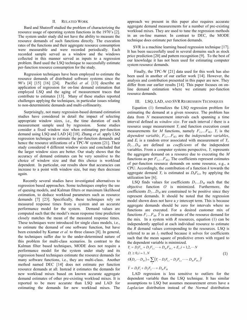
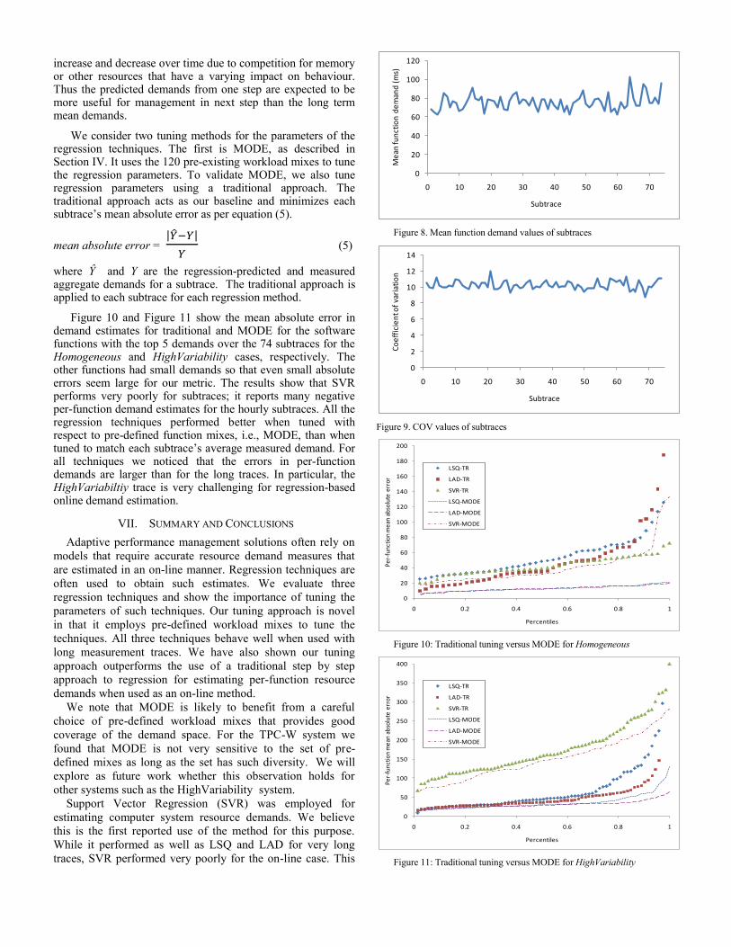
Figure 8 and Figure 9 show the mean function demand and COV of function demands for the 74 subtraces of the HighVariability case. As seen in the figure, the per-subtrace behaviour varies considerably with respect to overall mean demand. Hourly mean per-function demands, as averaged over the 50,000 function invocations, varied between 60 and 100 ms. The purpose of on-line demand estimation is to predict the per-function demands for each subtrace.

We note that the variation in demands illustrated in Figure 8 are random and due to the randomly generated high COV of demands for this case. In a real system we can expect temporal correlations in resource demand patterns between successive measurement intervals. For example, the demands may

Figure 5. SVR mean absolute errors for C and - TPC-W

Figure 6. SVR mean absolute errors for C and - Homogeneous

Figure 7. SVR mean absolute errors for C and - HighVariability

Table 2. Measured and estimated per-function demands for LSQ, LAD, and SVR

Function 1 2 3 4 5 6 7 8 9 10 11 12 13 14

Homogenous Measured 400.0 100.0 60.0 50.0 30.0 15.0 15.0 15.0 15.0 15.0 15.0 15.0 15.0 5.0

LSQ 399.1 101.9 57.9 36.8 0.0 16.1 16.5 38.8 15.5 14.5 13.2 0.0 29.3 32.4

LAD 396.7 101.0 59.7 52.2 0.0 12.1 17.1 0.0 13.5 15.3 15.4 35.5 11.7 28.8

SVR 400.5 102.5 59.4 46.5 9.8 16.1 14.4 15.5 15.0 14.6 19.2 113.6 -82.6 19.3

HighVariability Measured 1084.2 102.9 56.6 55.9 29.7 14.2 13.7 13.5 13.1 12.9 12.7 12.6 12.2 2.3

LSQ 1036.0 106.5 68.3 60.5 45.6 25.4 1.4 0.0 20.8 0.0 17.8 0.0 0.0 0.0

LAD 1032.5 112.2 67.9 55.3 0.0 36.0 0.0 0.0 29.7 0.0 9.1 0.0 0.0 66.3

SVR 1091.7 102.9 67.7 95.8 30.1 29.8 19.7 10.0 58.3 1.9 19.4 11.4 21.0 32.8

2^

-10

2^

-8

2^

-6

2^

-4

2^

-2

2^

0

2^

2

2^

4

2^

6

2^

8

0

20

40

60

80

100

120

140

160

180

2^-10

2^-6

2^-2

cost

Me

an a

bso

lute

err

or

ν

2^-6 2^-4 2^-2 2^0 2^2 2^4 2^6

0

10

20

30

40

50

60

2^-10

2^-7

2^-4

2^-1

cost

Me

an a

bso

lute

err

or

ν

2^-6 2^-4 2^-2 2^0 2^2 2^4 2^6

0

200

400

600

800

1000

1200

1400

2^-10

2^-7

2^-4

2^-1

cost

me

an a

bso

lute

err

or

ν

increase and decrease over time due to competition for memory or other resources that have a varying impact on behaviour. Thus the predicted demands from one step are expected to be more useful for management in next step than the long term mean demands.

We consider two tuning methods for the parameters of the regression techniques. The first is MODE, as described in Section IV. It uses the 120 pre-existing workload mixes to tune the regression parameters. To validate MODE, we also tune regression parameters using a traditional approach. The traditional approach acts as our baseline and minimizes each subtrace’s‎mean‎absolute error as per equation (5).

mean absolute error =

(5)

where Ŷ and Y are the regression-predicted and measured aggregate demands for a subtrace. The traditional approach is applied to each subtrace for each regression method.

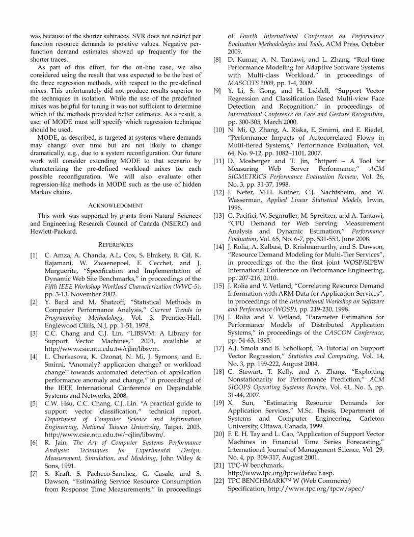
Figure 10 and Figure 11 show the mean absolute error in demand estimates for traditional and MODE for the software functions with the top 5 demands over the 74 subtraces for the Homogeneous and HighVariability cases, respectively. The other functions had small demands so that even small absolute errors seem large for our metric. The results show that SVR performs very poorly for subtraces; it reports many negative per-function demand estimates for the hourly subtraces. All the regression techniques performed better when tuned with respect to pre-defined function mixes, i.e., MODE, than when tuned‎to‎match‎each‎subtrace’s‎average‎measured‎demand.‎For‎all techniques we noticed that the errors in per-function demands are larger than for the long traces. In particular, the HighVariabiltiy trace is very challenging for regression-based online demand estimation.

VII. SUMMARY AND CONCLUSIONS

Adaptive performance management solutions often rely on

models that require accurate resource demand measures that

are estimated in an on-line manner. Regression techniques are

often used to obtain such estimates. We evaluate three

regression techniques and show the importance of tuning the

parameters of such techniques. Our tuning approach is novel

in that it employs pre-defined workload mixes to tune the

techniques. All three techniques behave well when used with

long measurement traces. We have also shown our tuning

approach outperforms the use of a traditional step by step

approach to regression for estimating per-function resource

demands when used as an on-line method.

We note that MODE is likely to benefit from a careful

choice of pre-defined workload mixes that provides good

coverage of the demand space. For the TPC-W system we

found that MODE is not very sensitive to the set of pre-

defined mixes as long as the set has such diversity. We will

explore as future work whether this observation holds for

other systems such as the HighVariability system.

Support Vector Regression (SVR) was employed for

estimating computer system resource demands. We believe

this is the first reported use of the method for this purpose.

While it performed as well as LSQ and LAD for very long

traces, SVR performed very poorly for the on-line case. This

Figure 8. Mean function demand values of subtraces

Figure 9. COV values of subtraces

Figure 10: Traditional tuning versus MODE for Homogeneous

Figure 11: Traditional tuning versus MODE for HighVariability

0

20

40

60

80

100

120

0 10 20 30 40 50 60 70

Me

an fu

nct

ion

de

man

d (

ms)

Subtrace

0

2

4

6

8

10

12

14

0 10 20 30 40 50 60 70

Co

eff

icie

nt o

f va

riat

ion

Subtrace

0

20

40

60

80

100

120

140

160

180

200

0 0.2 0.4 0.6 0.8 1

Per-

func

tion

mea

n ab

solu

te e

rror

Percentiles

LSQ-TR

LAD-TR

SVR-TR

LSQ-MODE

LAD-MODE

SVR-MODE

0

50

100

150

200

250

300

350

400

0 0.2 0.4 0.6 0.8 1

Per-

func

tion

mea

n ab

solu

te e

rror

Percentiles

LSQ-TR

LAD-TR

SVR-TR

LSQ-MODE

LAD-MODE

SVR-MODE

was because of the shorter subtraces. SVR does not restrict per

function resource demands to positive values. Negative per-

function demand estimates showed up frequently for the

shorter traces.

As part of this effort, for the on-line case, we also

considered using the result that was expected to be the best of

the three regression methods, with respect to the pre-defined

mixes. This unfortunately did not produce results superior to

the techniques in isolation. While the use of the predefined

mixes was helpful for tuning it was not sufficient to determine

which of the methods provided better estimates. As a result, a

user of MODE must still specify which regression technique

should be used.

MODE, as described, is targeted at systems where demands

may change over time but are not likely to change

dramatically, e.g., due to a system reconfiguration. Our future

work will consider extending MODE to that scenario by

characterizing the pre-defined workload mixes for each

possible reconfiguration. We will also evaluate other

regression-like methods in MODE such as the use of hidden

Markov chains.

ACKNOWLEDGMENT

This work was supported by grants from Natural Sciences

and Engineering Research Council of Canada (NSERC) and

Hewlett-Packard.

REFERENCES

[1] C. Amza, A. Chanda, A.L. Cox, S. Elnikety, R. Gil, K. Rajamani, W. Zwaenepoel, E. Cecchet, and J. Marguerite, “Specification and Implementation of Dynamic Web Site Benchmarks,” in proceedings of the Fifth IEEE Workshop Workload Characterization (WWC-5), pp. 3-13, November 2002.

[2] Y. Bard and M. Shatzoff, “Statistical Methods in Computer Performance Analysis,” Current Trends in Programming Methodology, Vol. 3, Prentice-Hall, Englewood Cliffs, N.J, pp. 1-51, 1978.

[3] C.C. Chang and C.J. Lin, “LIBSVM: A Library for Support Vector Machines,“ 2001, available at http://www.csie.ntu.edu.tw/cjlin/libsvm.

[4] L. Cherkasova, K. Ozonat, N. Mi, J. Symons, and E. Smirni, “Anomaly? application change? or workload change? towards automated detection of application performance anomaly and change,“ in proceedingd of the IEEE International Conference on Dependable Systems and Networks, 2008.

[5] C.W. Hsu, C.C. Chang, C.J. Lin. “A practical guide to support vector classification,“ technical report, Department of Computer Science and Information Engineering, National Taiwan University, Taipei, 2003. http://www.csie.ntu.edu.tw/~cjlin/libsvm/.

[6] R. Jain, The Art of Computer Systems Performance Analysis: Techniques for Experimental Design, Measurement, Simulation, and Modeling, John Wiley & Sons, 1991.

[7] S. Kraft, S. Pacheco-Sanchez, G. Casale, and S. Dawson, “Estimating Service Resource Consumption from Response Time Measurements,” in proceedings

of Fourth International Conference on Performance Evaluation Methodologies and Tools, ACM Press, October 2009.

[8] D. Kumar, A. N. Tantawi, and L. Zhang, “Real-time Performance Modeling for Adaptive Software Systems with Multi-class Workload,” in proceedings of MASCOTS 2009, pp. 1-4, 2009.

[9] Y. Li, S. Gong, and H. Liddell, “Support Vector Regression and Classification Based Multi-view Face Detection and Recognition,” in proceedings of International Conference on Face and Gesture Recognition, pp. 300-305, March 2000.

[10] N. Mi, Q. Zhang, A. Riska, E. Smirni, and E. Riedel, “Performance Impacts of Autocorrelated Flows in Multi-tiered Systems,” Performance Evaluation, Vol. 64, No. 9-12, pp. 1082–1101, 2007.

[11] D. Mosberger and T. Jin, “httperf – A Tool for Measuring Web Server Performance,” ACM SIGMETRICS Performance Evaluation Review, Vol. 26, No. 3, pp. 31-37, 1998.

[12] J. Neter, M.H. Kutner, C.J. Nachtsheim, and W. Wasserman, Applied Linear Statistical Models, Irwin, 1996.

[13] G. Pacifici, W. Segmuller, M. Spreitzer, and A. Tantawi, “CPU Demand for Web Serving: Measurement Analysis and Dynamic Estimation,” Performance Evaluation, Vol. 65, No. 6-7, pp. 531-553, June 2008.

[14] J. Rolia, A. Kalbasi, D. Krishnamurthy, and S. Dawson, “Resource Demand Modeling for Multi-Tier Services”, in proceedings of the the first joint WOSP/SIPEW International Conference on Performance Engineering, pp. 207-216, 2010.

[15] J. Rolia and V. Vetland, “Correlating Resource Demand Information with ARM Data for Application Services”, in proceedings of the International Workshop on Software and Performance (WOSP), pp. 219-230, 1998.

[16] J. Rolia and V. Vetland, “Parameter Estimation for Performance Models of Distributed Application Systems,” in proceedings of the CASCON Conference, pp. 54-63, 1995.

[17] A.J. Smola and B. Scholkopf, “A Tutorial on Support Vector Regression,” Statistics and Computing, Vol. 14, No. 3, pp. 199-222, August 2004.

[18] C. Stewart, T. Kelly, and A. Zhang, “Exploiting Nonstationarity for Performance Prediction,” ACM SIGOPS Operating Systems Review, Vol. 41, No. 3, pp. 31-44, 2007.

[19] X. Sun, “Estimating Resource Demands for Application Services,” M.Sc. Thesis, Department of Systems and Computer Engineering, Carleton University, Ottawa, Canada, 1999.

[20] F. E. H. Tay and L. Cao, “Application of Support Vector Machines in Financial Time Series Forecasting,” International Journal of Management Science, Vol. 29, No. 4, pp. 309-317, August 2001.

[21] TPC-W benchmark, http://www.tpc.org/tpcw/default.asp.

[22] TPC BENCHMARKTM W (Web Commerce) Specification, http://www.tpc.org/tpcw/spec/

tpcw_V1.8.pdf. [23] M. Woodside, T. Zhen, and M. Litoiu, “Service System

Resource Management Based on a Tracked Layered Performance Model,” in proceedings of the International Conference on Autonomic Computing, pp. 175-184, 2006.

[24] Q. Zhang L. Cherkasova, N. Mi, and E. Smirni, “A Regression-Based Analytic Model for Capacity Planning of Multi-Tier Applications,” in proceedings of Fourth IEEE International Conference on Autonomic Computing, June 2007.