61
Model Assessment and Selection in Multiple and Multivariate Regression Ho Tu Bao Japan Advance Institute of Science and Technology John von Neumann Institute, VNU-HCM

Model Assessment and Selection in Multiple and Multivariate Regression
Ho Tu Bao
Japan Advance Institute of Science and Technology
John von Neumann Institute, VNU-HCM

Statistics and machine learning
Statistics Long history, fruitful
Aims to analyze datasets
Early focused on numerical data
Multivariate analysis = linear methods on small to medium-sized data sets + batch processing.
1970s: interactive computing + exploratory data analysis (EDA)
Computing power & data storage machine learning and data mining (aka EDA extension).
Statisticians interested in ML
Machine learning Newer, fast development
Aims to exploit datasets to learn
Early focused on symbolic data
Tends closely to data mining (more practical exploitation of
large datasets
Increasing employs statistical methods
More practical with computing power
ML people: need to learn statistics!
2

Outline
1. Introduction
2. The Regression Function and Least Squares
3. Prediction Accuracy and Model Assessment
4. Estimating Predictor Error
5. Other Issues
6. Multivariate Regression
3 Hesterberg et al., LARS and l1 penalized regression

Introduction Model and modeling
4
Model:
Mô tả khái quát hoặc trừu tượng hóa của một thực thể (simplified description or abstraction of a reality).
Modeling: Quá trình tạo ra một mô hình.
Mathematical modeling: Description of a system using mathematical concepts and language
Linear vs. nonlinear; deterministic vs. probabilistic; static vs. dynamic; discrete vs. continuous; deductive, inductive, or floating.
A method for model assessment and selection
Model selection: Select the most appropriate model
Given the problem target and the data Choose appropriate methods and parameter settings for the most appropriate model.
No free lunch theorem.

Introduction History
The earliest form of regression was the method of least squares which was published by Legendre in 1805 and by Gauss in 1809.
The term “regression” coined by Francis Galton in the 19th century to describe a biological phenomenon which was extended by Udny Yule and Karl Pearson to a more general statistical context (1897, 1903).
In 1950s, 1960s, economists used electromechanical desk calculators to calculate regressions. Before 1970, it sometimes took up to 24 hours to receive the result from one regression.
Regression methods continue to be an area of active research. In recent decades, new methods have been developed for robust regression in , time series, images, graphs, or other complex data objects, nonparametric regression, Bayesian methods for regression, etc.
5

Introduction Regression and model
Given 𝐗𝑖, 𝐘𝑖 , 𝑖 = 1, … , 𝑛 where each 𝐗𝑖 is a vector of r random
variables 𝐗 = (𝑋1, … , 𝑋𝑟)𝜏 in a space 𝕏 and 𝐘i is a vector of s random
variables 𝐘 = (𝑌1, … , 𝑌𝑠)𝜏 in a space 𝕐
The problem is to learn a function 𝑓: 𝕏 ⟶ 𝕐 from 𝐗𝑖, 𝐘𝑖 , 𝑖 = 1, … , 𝑛 satisfies 𝑓 𝐗𝑖 = 𝐘𝑖 , 𝑖 = 1, … , 𝑛.
When 𝕐 is discrete the problem is called classification and when 𝕐 is continuous the problem is called regression. For regression:
When r = 1 and s =1 the problem is called simple regression.
When r > 1 and s =1 the problem is called multiple regression.
When r > 1 and s > 1 the problem is called multivariate regression.
6
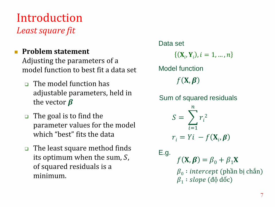
Introduction Least square fit
Problem statement Adjusting the parameters of a model function to best fit a data set
The model function has adjustable parameters, held in the vector 𝜷
The goal is to find the parameter values for the model which “best” fits the data
The least square method finds its optimum when the sum, 𝑆, of squared residuals is a minimum.
7
𝑓 𝐗, 𝜷
𝑆 = 𝑟𝑖2
𝑛
𝑖=1
𝑟𝑖 = 𝑌𝑖 − 𝑓 𝐗𝑖, 𝜷
Data set
Model function
Sum of squared residuals
E.g. 𝑓 𝐗, 𝜷 = 𝛽0 + 𝛽1𝐗
𝛽0 ∶ 𝑖𝑛𝑡𝑒𝑟𝑐𝑒𝑝𝑡 (phần bị chắn) 𝛽1 ∶ 𝑠𝑙𝑜𝑝𝑒 (độ dốc)
𝐗𝑖, 𝐘𝑖 , 𝑖 = 1, … , 𝑛

Introduction Least square fit
Solving the problem
Minimum of the sum of squared residuals is found by setting the gradient to zero.
The gradient equations apply to all least squares problems.
Each particular problem requires particular expression for the model and its partial derivatives.
𝜕𝑆
𝜕𝛽𝑗
= 2 𝑟𝑖
𝜕𝑟𝑖
𝜕𝛽𝑖
= 0,
𝑖
𝑗 = 1, … , 𝑚
Gradient on 𝛽
𝑟𝑖 = 𝑌𝑖 −
𝑓 𝐗𝑖, 𝜷
−2 𝑟𝑖
𝜕𝑓 𝐗𝑖, 𝜷
𝜕𝛽𝑗
= 0,
𝑖
𝑗 = 1, … , 𝑚
Gradient equation

Introduction Least square fit
Linear least squares
Coefficients 𝜑𝑖 are functions of X𝑖
Non-linear least squares
There is no closed-form solution to a non-linear least squares problem.
Numerical algorithms are used to find the value of the parameter 𝜷 which minimize the objective.
The parameters 𝜷 are refined iteratively and the values are obtained by successive approximation.
𝑓 𝐗𝑖, 𝜷 = 𝛽𝑗 𝜑𝑗 𝐗𝑖
𝑚
𝑗=1
Linear model function
𝑿𝑖𝑗 = 𝜕𝑓 𝐗𝑖, 𝜷
𝜕𝛽𝑗 = 𝜑𝑗 𝐗𝑖
𝜷 = 𝐗𝑇 𝐗 −1 𝐗𝑇 𝒀
Iterative approximation
𝛽𝑗𝑘+1 = 𝛽𝑗
𝑘 + ∆𝛽𝑗
Shift vector
𝑓 𝐗𝑖, 𝜷 = 𝑓𝑘 𝐗𝑖, 𝜷 + 𝜕𝑓 𝐗𝑖, 𝜷
𝜕𝛽𝑗
𝛽𝑗 − 𝛽𝑗𝑘
𝑚
𝑗=1
= 𝑓𝑘 𝐗𝑖, 𝜷 + 𝐽𝑖𝑗 ∆𝛽𝑗
𝑚
𝑗=1
Gradient equation
−2 𝐽𝑖𝑗 ∆𝑌𝑖 − 𝐽𝑖𝑗 ∆𝛽𝑗
𝑚
𝑗=1
= 0
𝑛
𝑖=1
Gauss-Newton algorithm
an expression is said to be a closed-form expression if it can be expressed
analytically in terms of a finite number of certain "well-known" functions.
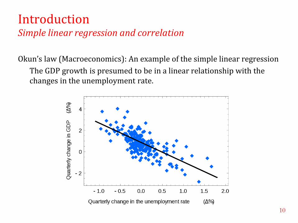
Introduction Simple linear regression and correlation
Okun’s law (Macroeconomics): An example of the simple linear regression
The GDP growth is presumed to be in a linear relationship with the changes in the unemployment rate.
10

Introduction Simple linear regression and correlation
Correlation analysis (correlation coefficient) is for determining whether a relationship exists.
Simple linear regression is for examining the relationship between two variables (if a linear relationship between them exists).
Mathematical equations describing these relationships are models, and they fall into two types: deterministic or probabilistic.
Deterministic model: an equation or set of equations that allow us to fully determine the value of the dependent variable from the values of the independent variables.
Contrast this with…
Probabilistic model: a method used to capture the randomness that is part of a real-life process.
11

Introduction Simple linear regression
Example: Do all houses of the same size sell for exactly the same price?
Models
Deterministic model: approximates the relationship we want to model and add a random term that measures the error of the deterministic component.
The cost of building a new house is about $75 per square foot and most lots sell for about $25,000. Hence the approximate selling price (Y) would be:
Y = $25,000 + (75$/ft2)(X)
(where X is the size of the house in square feet)
12

Introduction Background of model design
The facts
Having too many input variables in the regression model ⇒ an overfitting regression function with an inflated variance
Having too few input variables in the regression model ⇒ an underfitting and high bias regression function with poor explanation of the data
The “importance” of a variable
Depends on how seriously it will affects prediction accuracy if it is dropped.
The behind driving force
The desire for a simpler and more easily interpretable regression model combined with a need for greater accuracy in prediction.
13

Introduction Simple linear regression
A model of the relationship between house size (independent variable) and house price (dependent variable) would be:
In this model, the price of the house is completely determined by the size
14
House size
House Price
Most lots sell
for $25,000
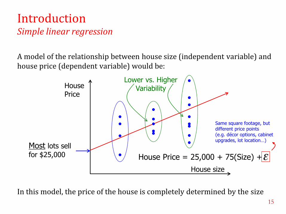
Introduction Simple linear regression
A model of the relationship between house size (independent variable) and house price (dependent variable) would be:
In this model, the price of the house is completely determined by the size
15
House size
House Price
Most lots sell
for $25,000
Lower vs. Higher Variability
House Price = 25,000 + 75(Size) +
Same square footage, but different price points (e.g. décor options, cabinet upgrades, lot location…)

Introduction Simple linear regression
Example: Do all houses of the same size sell for exactly the same price?
Probabilistic model:
𝑌 = 25,000 + 75 𝐗 + 𝜀
where 𝜀 is the random term (error variable). It is the difference between the actual selling price and the estimated price based on the size of the house. Its value will vary from house sale to house sale, even if the square footage (X) remains the same.
First order simple linear regression model:
𝑌 = 𝛽0 + 𝜷1𝑿 + 𝜀
16
Dependent variable
intercept slope
independent variable
error variable

Introduction Regression and model
Techniques for modeling and analyzing the relationship between dependent variables and independent variables.
17
𝑿𝑖 =𝑋1
𝑖
⋮𝑋𝑟
𝑖 𝒀𝑖 =
𝑌1𝑖
⋮𝑌𝑠
𝑖
Input (independent, predictor, explanatory) Output (dependent, predicted, response)
The relationship = Regression model
Different forms of
𝑓: 𝕏 ⟶ 𝕐
linear vs. nonlinear,
parametric vs. nonparametric.
Linear combination of the parameters (but need not be linear in the independent variables)

Introduction Model selection and model assessment
Model Selection: Estimating performances of different models to choose the best one (produces the minimum of the test error).
Model Assessment: Having chosen a model, estimating the prediction error on new data.
18

Outline
1. Introduction
2. The Regression Function and Least Squares
3. Prediction Accuracy and Model Assessment
4. Estimating Predictor Error
5. Other Issues
6. Multivariate Regression
19

Regression function and least squares
Consider the problem of predicting 𝑌 by a function, 𝑓 𝐗 , of 𝐗
Loss function
𝐿 𝑌, 𝑓 𝐗
measures the prediction accuracy gives the loss incurred if 𝑌 is predicted by 𝑓 𝐗 .
Risk function
𝑅 𝑓 = 𝐸 𝐿 𝑌, 𝑓 𝐗
(expected loss) measures the quality of 𝑓 𝐗 as a predictor.
Bayes rule and the Bayes risk
The Bayes rule is the function 𝑓∗ which minimizes 𝑅 𝑓 , and the Bayes risk is 𝑅 𝑓∗ .
20

Regression function and least squares Regression function
Squared-error loss function
𝐿 𝑌, 𝑓 𝐗 = 𝑌 − 𝑓 𝐗2
Mean square error criterion
𝑅 𝑓 = 𝐸 𝑌 − 𝑓 𝐗2
= 𝐸𝐗 𝐸𝑌 𝐗 𝑌 − 𝑓 𝐗2 𝐗
We can write Y − f(x) = (Y − μ(x)) + (μ(x) − f(x)) where
𝜇 𝐱 = 𝐸𝑌 𝐗 𝑌 𝐗 = 𝐱
is called regression function of Y on X . Squaring both sides and taking the conditional distribution of 𝑌 given 𝐗 = 𝐱, as 𝐸𝑌 𝐗 𝑌 − 𝜇(𝑥) 𝐗 = 𝐱 = 0,
we have
𝐸𝑌 𝐗 𝑌 − 𝑓 𝐗2 𝐗 = 𝐱 = 𝐸𝑌 𝐗 𝑌 − 𝜇 𝐱
2 𝐗 = 𝐱 + 𝜇 𝐱 − 𝑓 𝐱
𝟐
21

Regression function and least squares Least squares
Taking 𝑓∗ 𝐱 = 𝜇 𝐱 = 𝐸𝑌 𝑋*𝑌 𝐗 = 𝐱+, the
previous equation is minimized
𝐸𝑌 𝐗*(𝑌 − 𝑓∗ 𝐱 )2|𝐗 = 𝐱+
= 𝐸𝑌 𝐗*(𝑌 − 𝜇 𝐱 )2 𝐗 = 𝐱+
Taking expectations of both sides, we have Bayes risk
𝑅 𝑓∗ = min𝑓 𝑅 𝑓 = 𝐸 𝑌 − 𝜇 𝐗2
The regression function 𝜇 𝐗 of 𝑌 on 𝐗, evaluated at 𝐗 = 𝐱, is the “best” predictor (defined by using minimum mean squared error).
22
Data
Statistical
model
Systematic
component
+
Random
errors

Regression function and least squares
Assumption
The output variables 𝒀 are linearly related to the input variables 𝑿
The model 𝜇 𝐗 = 𝛽0 + 𝛽𝑖 𝑿𝑖
𝑟𝑖=1 ⟹ 𝑌 = 𝛽0 + 𝛽𝑖 𝑿𝑖
𝑟𝑖=1 + 𝑒
is treated depending on assumptions on how 𝑋1, … , 𝑋𝑟 were generated.
𝑿𝑖 : the input (or independent, predictor) variables 𝑌: the output (or dependent, response) variable 𝑒 : (error) the unobservable random variable with mean 0, variance 2ߪ
The tasks
To estimate the true values of 𝛽0, 𝛽1, … , 𝛽𝑟 , and 2ߪ To assess the impact of each input variable on the behavior of 𝑌 To predict future values of 𝑌 To measure the accuracy of the predictions
23

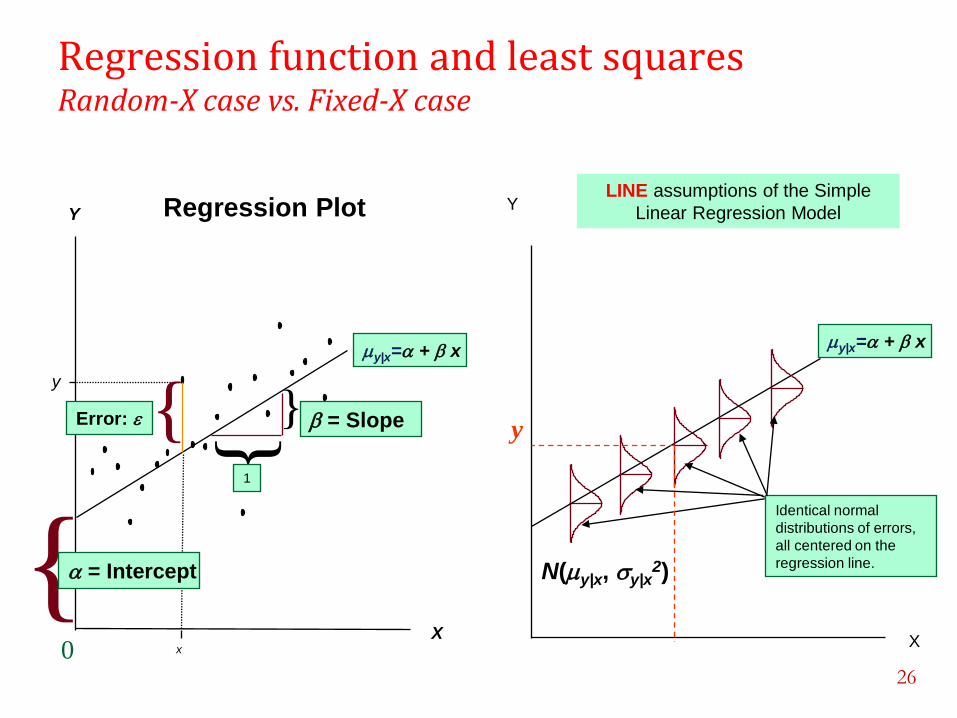
Regression function and least squares Random-X case vs. Fixed-X case
Random-X case
X is a random variable, also known as the structural model or structural relationship.
Methods for the structural model require some estimate of the variability of the variable X.
The least squares fit will still give the best linear predictor of Y, but the estimates of the slope and intercept will be biased.
E(Y|X) = β0 + β1X
Fixed-X case (Fisher, 1922)
X is fixed, but measured with noise, is known as the functional model or functional relationship.
The fixed-X assumption is that the explanatory variable is measured without error.
Distribution of the regression coefficient is unaffected by the distribution of X.
E(Y|X=x) = β0 + β1x
24

Regression function and least squares Random-X case vs. Fixed-X case
25
Regression function and least squares Random-X case vs. Fixed-X case
26
Regression Plot
0 X
Y
my|x=a + x
x
} }
= Slope
1
y
{ Error:
{ a = Intercept
X
Y LINE assumptions of the Simple
Linear Regression Model
Identical normal
distributions of errors,
all centered on the
regression line.
my|x=a + x
y
N(my|x, sy|x2)

Regression function and least squares Random-X case
Regression coefficients
𝜷 =𝛽1
⋮𝛽𝑟
, 𝜶 =
𝛽0
𝛽1
⋮𝛽𝑟
, 𝐙 =
1𝑿1
⋮𝑿𝑟
Regression function
𝜇 𝐗 = 𝐙𝜏𝜶 = 𝛽0 + 𝜷𝐗 = 𝛽0 + 𝛽𝑗 𝑿𝑗𝑟𝑗=1
Let
𝑆 𝜶 = 𝐸 𝑌 − 𝐙𝜏𝜶 2
and define 𝜶∗ = arg min𝜶 𝑆 𝜶
27

Regression function and least squares Random-X case
Setting differential of 𝑆 𝜶 with respect to 𝜶 to 0
𝜕𝑆 𝜶
𝜕𝜶= −2𝐸 𝐙𝑌 − 𝐙𝐙𝜏𝜶 = 0
We get 𝜶∗= E 𝐙𝐙τ −1E 𝐙𝑌
𝜷∗= 𝚺𝑋𝑋−1𝚺𝑋𝑌, 𝛽0
∗ = 𝜇𝑌 − 𝝁𝑋𝜏 𝜷∗
In practice, 𝝁𝑋, 𝜇𝑌, 𝚺𝑋𝑋, and 𝚺𝑋𝑌 are unknown, we estimate them by ML
using data generated by the joint distribution of 𝐗, 𝑌 . Let
𝒳 = (X1, · · · ,Xn)τ, 𝒴 = (Y1, · · · , Yn)τ, 𝐗 =1
𝑛 𝐗𝑗
n1 , 𝑌 =
1
𝑛 𝑌𝑗
𝑛1 ,
𝒳 = 𝐗 , … , 𝐗 𝜏, 𝒴 = 𝑌 , … , 𝑌 𝜏, 𝒳𝑐 = 𝒳 − 𝒳 , 𝒴𝑐 = 𝒴 − 𝒴 ,
𝜷 ∗ = 𝒳𝑐𝜏𝒳𝑐
−1𝒳𝑐𝜏𝒴𝑐 , 𝛽 0
𝜏 = 𝑌 − 𝐗 𝜏𝜷 ∗
28 Covariance matrix: ΣXX = cov(X,X) = E{(X − μX)(X − μX)τ }

Regression function and least squares Fixed-X case
𝑋1, … , 𝑋𝑟 are fixed in repeated sampling and 𝑌 may be selected in the designed experiment or 𝑌 may be observed conditional on the 𝑋1, … , 𝑋𝑟
𝒵 =1 𝑋1
1 ⋯ 𝑋𝑟1
⋮ ⋮ ⋱ ⋮1 𝑋1
𝑛 ⋯ 𝑋𝑟𝑛
- input variables, 𝒴 =𝑌1
⋮𝑌𝑟
- output variables
The regression function
𝑌𝑖 = 𝛽0 + 𝛽𝑗𝑋𝑖𝑗 + 𝑒𝑖
𝑟
𝑗=1
, 𝑖 = 1,2, … , 𝑛
𝒴 = 𝒵𝜷 + 𝒆
𝒆: random n-vector of unobservable errors with 𝐸 𝒆 = 0, var 𝒆 = 𝜎2𝐈𝑛 .
Error sum of squares
𝐸𝑆𝑆 𝜷 = e𝑖2 = 𝒆𝜏𝒆 = (𝒴 − 𝒵𝜷)𝜏𝑛
𝑖=1 (𝒴 − 𝒵𝜷)
29

Regression function and least squares Fixed-X case
Estimate 𝜷 by minimizing 𝐸𝑆𝑆 𝜷 w.r.t. 𝜷. Set differential w.r.t. 𝜷 to 0
𝜕𝐸𝑆𝑆(𝜷)
𝜕𝜷= −2𝒵𝜏 𝒴 − 𝒵𝜷 = 0
The unique ordinary least-squares (OLS) estimator of 𝜷 is
𝜷 𝑜𝑙𝑠 = (𝒵𝜏𝒵)−1𝒵𝜏𝒴
Even though the descriptions differ as to how the input data are generated, the ordinary least-squares estimator estimates turn out to be the same for the random-X case and the fixed-X case:
𝜷 ∗ = 𝒳𝑐𝜏𝒳𝑐
−1𝒳𝑐𝜏𝒴𝑐 , 𝛽 0
𝜏 = 𝑌 − 𝐗 𝜏𝜷 ∗
The components of the n-vector of OLS fitted values are the vertical projections of the n points onto the LS regression surface (or hyperplane)
𝑌 𝑖 = 𝜇 𝐗𝑖 = 𝐗𝑖𝜏𝜷 𝑜𝑙𝑠, 𝑖 = 1, … , 𝑛.
30

Regression function and least squares Fixed-X case
The variance of 𝑌 𝑖 for fixed Xi is given by
var 𝑌 𝑖 𝐗𝑖 = 𝐗𝑖𝜏 𝑣𝑎𝑟(𝛽 𝑜𝑙𝑠) 𝐗𝑖 = 𝜎2𝐗𝑖
𝜏(𝒵𝜏𝒵)−1𝐗𝑖
The n-vector of fitted values 𝒴 = (𝑌 1, … , 𝑌 𝑛)𝜏 is
𝒴 = 𝒵𝜷 𝑜𝑙𝑠 = 𝒵(𝒵𝜏𝒵)−1𝒵𝜏𝒴 = 𝐇𝒴
where the (n×n)-matrix H = 𝒵(𝒵𝜏𝒵)−1𝒵𝜏 is often called the hat matrix.
The variance of Y is given by
𝑣𝑎𝑟 𝒴 𝐗 = 𝐻 𝑣𝑎𝑟 𝒴 𝐇𝜏 = 𝜎2H
The residuals, 𝒆 = 𝒴 − 𝒴 = (In − H)𝒴 are the
OLS estimates of the unobservable errors e,
and can be written as 𝒆 = 𝐈𝑛 − 𝐇 𝒆.
31

Regression function and least squares ANOVA table for multiple regression model and F-statistic
Residual variance 𝜎 2 =𝑅𝑆𝑆
𝑛−𝑟−1
Total sum of squares 𝑆𝑌𝑌= (𝑛𝑖=1 𝑌𝑖 − 𝑌 )2 = 𝒴 − 𝒴 𝜏 𝒴 − 𝒴
Regression sum of 𝑆𝑆𝑟𝑒𝑔 = (𝑛𝑖=1 𝑌 𝑖 − 𝑌 𝑖)
2 = 𝛽 𝑜𝑙𝑠𝜏 (𝒵𝜏𝒵)𝛽 𝑜𝑙𝑠
of squares
Residual sum of squares 𝑅𝑆𝑆 = (𝑛𝑖=1 𝑌𝑖 − 𝑌 𝑖)
2 = (𝒴 − 𝒵𝛽 𝑜𝑙𝑠)𝜏(𝒴 − 𝒵𝛽 𝑜𝑙𝑠)
Use F-statistic, 𝐹 =𝑆𝑆𝑟𝑒𝑔 𝑟
𝑅𝑆𝑆 (𝑛−𝑟−1) , to see if there is a linear relationship
between Y and the Xs: F small not reject 𝛽 = 0, F large ∃𝑗, 𝛽𝑗 ≠ 0.
If 𝛽𝑗= 0, use t-statistic, 𝑡𝑗 =𝛽 𝑗
𝜎 𝑣𝑗𝑗, where 𝑣𝑗𝑗 is the jth diagonal entry of
(𝒵𝜏𝒵)−1. If 𝑡𝑗 large large 𝛽𝑗 ≠ 0, else (near zero) 𝛽𝑗 = 0. 32

Regression function and least squares Bodyfat data
n = 252 men, to relate the percentage of bodyfat to age, weight, height, neck, chest, abdomen, hip, thigh, knee, ankle, bicept, foream, wrist (13).
33
bodyfat = β0 + β1(age)
+ β2(weight) + β3(height)
+ β4(neck) + β5(chest)
+ β6(abdomen) + β7(hip)
+ β8(thigh) + β9(knee)
+ β10(ankle)
+ β11(biceps)
+ β12(forearm)
+ β13(wrist) + e
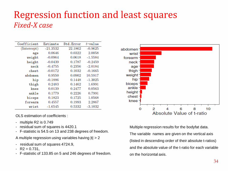
Regression function and least squares Fixed-X case
34
OLS estimation of coefficients :
- multiple R2 is 0.749
- residual sum of squares is 4420.1
- F-statistic is 54.5 on 13 and 238 degrees of freedom.
A multiple regression using variables having |t| > 2
- residual sum of squares 4724.9,
- R2 = 0.731,
- F-statistic of 133.85 on 5 and 246 degrees of freedom.
Multiple regression results for the bodyfat data.
The variable names are given on the vertical axis
(listed in descending order of their absolute t-ratios)
and the absolute value of the t-ratio for each variable
on the horizontal axis.

Outline
1. Introduction
2. The Regression Function and Least Squares
3. Prediction Accuracy and Model Assessment
4. Estimating Predictor Error
5. Other Issues
6. Multivariate Regression
35

Prediction accuracy and model assessment
The aims
Prediction is the art of making accurate guesses about new response values that are independent of the current data.
Good predictive ability is often recognized as the most useful way of assessing the fit of a model to data.
Practice
Learning data ℒ = * 𝐗𝑖 , 𝑌𝑖 , 𝑖 = 1, … , 𝑛+ for regression of 𝑌 on 𝑿.
Prediction of a new 𝑌𝑛𝑒𝑤 by applying the fitted model to a brand-new 𝑿𝑛𝑒𝑤 , from the test set 𝑇.
Predicted 𝑌𝑛𝑒𝑤 is compared with the actual response value. The predictive ability of the regression model is assessed by its prediction error (or generalization error), an overall measure of the quality of the prediction, usually taken to be mean squared error.
36

Prediction accuracy and model assessment Random-X case
Learning data set 𝐿 = 𝐗𝑖, 𝑌𝑖 , 𝑖 = 1, … , 𝑛 are observations from the
joint distribution of 𝐗, 𝑌 and
𝑌 = 𝛽0 + 𝛽𝑗 𝑋𝑗
𝑟
𝑗=1
+ 𝑒 = 𝜇 𝐗 + 𝑒
where 𝜇 𝐗 = 𝐸 𝑌 𝐗 , 𝐸 𝑒 𝐗 = 0, 𝑣𝑎𝑟 𝑒 𝐗 = 𝜎2
Given the test set 𝑇 = 𝐗𝑛𝑒𝑤, 𝑌𝑛𝑒𝑤 , if the estimated OLS regression
function at X is 𝜇 𝐗 = 𝛽 0 + 𝐗𝜏𝜷 𝑜𝑙𝑠
then the predicted value of 𝑌 at 𝐗new is 𝑌 = 𝜇 𝐗𝑛𝑒𝑤 .
37

Prediction accuracy and model assessment Random-X case
Prediction Error
𝑃𝐸𝑅 = 𝐸 𝑌𝑛𝑒𝑤 − 𝜇 𝐗𝑛𝑒𝑤 2 = 𝜎2 + 𝑀𝐸𝑅
Model Error (also called the “expected bias-squared”)
𝑀𝐸𝑅 = 𝐸 𝜇 𝐗𝑛𝑒𝑤 − 𝜇 𝐗𝑛𝑒𝑤 2 = 𝜷 − 𝜷 𝑜𝑙𝑠
𝜏𝚺𝑋𝑋 𝜷 − 𝜷 𝑜𝑙𝑠
38

Prediction accuracy and model assessment Fixed-X case
In 𝐿 = 𝐗𝑖, 𝑌𝑖 , 𝑖 = 1, … , 𝑛 , 𝑿𝑖 are fixed and only Y is random.
Assume that
𝑌𝑖 = 𝛽0 + 𝛽𝑗 𝑋𝑗𝑖
𝑟
𝑗=1
+ 𝑒𝑖 = 𝜇 𝐗𝑖 + 𝑒𝑖
where 𝜇 𝐗𝑖 = 𝛽0 + 𝛽𝑗 𝑋𝑗𝑖𝑟
𝑗=1 is the regression function evaluated at
𝐗𝑖 , and the errors 𝑒𝑖 are iid with mean 0 and variance
𝜎2 and uncorrelated with 𝑿𝑖 .
Assume the test data set generated by “future-fixed” 𝐗𝑛𝑒𝑤 and 𝑇 =
𝐗𝑖, 𝑌𝑖𝑛𝑒𝑤 , 𝑖 = 1, … , 𝑚 , where 𝑌𝑖
𝑛𝑒𝑤 = 𝜇 𝑋𝑖 + 𝑒𝑖𝑛𝑒𝑤 . The predicted
value of 𝑌𝑛𝑒𝑤at X is 𝜇 𝐗 = 𝛽 0 + 𝐗𝜏𝜷 𝑜𝑙𝑠.
39

Prediction accuracy and model assessment Fixed-X case
Prediction Error
𝑃𝐸𝐹 = 𝐸1
𝑚 𝑌𝑖
𝑛𝑒𝑤 − 𝜇 𝐗𝑖2
𝑚
𝑖=1
= 𝜎2 + 𝑀𝐸𝐹
Model Error
𝑀𝐸𝐹 =1
𝑚 𝑌𝑖
𝑛𝑒𝑤 − 𝜇 𝐗𝑖2
𝑚
𝑖=1
= 𝛽 − 𝛽 𝑜𝑙𝑠
𝜏 1
𝑚𝜒𝜏𝜒 Σ𝑋𝑋 𝛽 − 𝛽 𝑂𝐿𝑆
40

Outline
1. Introduction
2. The Regression Function and Least Squares
3. Prediction Accuracy and Model Assessment
4. Estimating Predictor Error
5. Other Issues
6. Multivariate Regression
41

42 Russ Greiner, ICML’04 PC co-chair
Observed from ICML 2004

Estimating prediction error Training, validation, and testing data
43
Data
Predictions
Y N
Results known
Training set
Validation set
+ + - - +
Model Builder
Evaluate
+
-
+
-
Final Model Final Test Set +
-
+
-
Final Evaluation
Model
Builder
Estimating prediction error Background
In cases the entire data set is not large enough and a division of the data into learning, validation, and test sets is not practical, we have to use alternative methods.
Apparent Error Rate
Applying the regression function obtained from OLS to the original sample data to see how well it predicts those same members
Cross-Validation
Split data set into two subsets, treating one subset as the learning set, and the other as the test set. Fit a model using this learning set and compute its prediction error. The learning set and the test set are then switched, and average all the prediction errors to estimate the test error.
44

Estimating prediction error Background
Bootstrap
Drawing a random sample with replacement having the same size as the parent data set. Fit a model using this bootstrap sample and compute its prediction error. Repeat the procedure, and average all the prediction errors to estimate the test error.
Random-X case: Cross-validation and “unconditional bootstrap” are appropriate;
Fixed-X case: “Conditional bootstrap” are appropriate but cross-validation is not appropriate for estimating prediction error.
45

Estimating prediction error
Apparent error rate (resubstitution error rate)
𝑃𝐸 𝜇 , 𝐷 =1
𝑛 𝑌𝑖
𝑛𝑒𝑤 − 𝜇 𝐗𝑖2
=𝑅𝑆𝑆
𝑛
𝑛
𝑖=1
Misleadingly optimistic, 𝑅𝑆𝑆 𝑛 will be PE too optimistic estimation with 𝑃𝐸 𝜇 , 𝐷 < 𝑃𝐸
Cross-Validation (V-fold)
𝐷 ⟹ 𝑇1, … , 𝑇𝑉 , 𝐷 = 𝑇𝑣𝑉𝑣=1 , 𝑇𝑣⋂𝑇𝑣′ = ∅
𝐿𝑣 = 𝐷 − 𝑇𝑣, 𝑃𝐸 𝐶𝑉/𝑉 =
1
𝑉 𝑌𝑖 − 𝜇 −𝑣 𝐗𝑖
2
𝐗𝑖𝑌𝑖 ∈𝑇𝑣
𝑉
𝑣=1
subtract 𝜎2 (obtain from the full data set) from 𝑃𝐸 to get 𝑀𝐸
Leave-one-out rule: 𝑉 = 𝑛, the most computationally intensive, but usually worse at model assessment than 10-fold (even 5-fold) CV.
46
1 2
3
da
ta 1 2 3
3 1 2
2 3 1
Training Testing
Random Partition
Learning
Average Error

Estimating prediction error
Bootstrap (Efron, 1979)
Unconditional Bootstrap
Random-X bootstrap sample (with replacement)
𝐷𝑅∗𝑏 = 𝐗𝑖
∗𝑏 , 𝑌𝑖∗𝑏 , 𝑖 = 1, … , 𝑛
𝑃𝐸 𝜇 𝑅∗𝑏 , 𝐷 =
1
𝑛 𝑌𝑖 − 𝜇 𝑅
∗𝑏 𝐗𝑖2
𝑛
𝑖=1
Simple bootstrap estimator of 𝑃𝐸
𝑃𝐸 𝑅 𝐷 =
1
𝐵 𝑃𝐸 𝜇 𝑅
∗𝑏 , 𝐷
𝐵
𝑏=1
=1
𝐵𝑛 𝑌𝑖 − 𝜇 𝑅
∗𝑏 𝐗𝑖2
𝑛
𝑖=1
𝐵
𝑏=1
Simple bootstrap estimator of 𝑃𝐸 using apparent error rate for 𝐷𝑅∗𝑏
𝑃𝐸 𝐷𝑅∗𝑏 =
1
𝐵 𝑃𝐸 𝜇 𝑅
∗𝑏 , 𝐷𝑅∗𝑏
𝐵
𝑏=1
=1
𝐵𝑛 𝑌𝑖
∗𝑏 − 𝜇 𝑅∗𝑏 𝐗𝑖
∗𝑏2
𝑛
𝑖=1
𝐵
𝑏=1
47

Estimating prediction error
Bootstrap
Unconditional Bootstrap
Simple estimators of 𝑃𝐸 are overly optimistic because there are
observations common to the bootstrap samples 𝐷𝑅∗𝑏 that
determined 𝜇 𝑅∗𝑏
The optimism (improvement of 𝑃𝐸 by estimating the bias for 𝐷𝑅∗𝑏
using 𝑅𝑆𝑆 𝑛 as an estimate of 𝑃𝐸 and then correcting 𝑅𝑆𝑆 𝑛 by subtracting its estimated bias)
𝑜𝑝𝑡 𝑅𝑏 = 𝑃𝐸 𝜇 𝑅
∗𝑏 , 𝐷 − 𝑃𝐸 𝜇 𝑅∗𝑏 , 𝐷𝑅
∗𝑏
𝑜𝑝𝑡 𝑅 =1
𝐵 𝑜𝑝𝑡 𝑅
𝑏
𝐵
𝑏=1
= 𝑃𝐸 𝑅 𝐷 − 𝑃𝐸 𝐷𝑅
∗𝑏
𝑃𝐸 𝑅 =
𝑅𝑆𝑆
𝑛+ 𝑜𝑝𝑡 𝑅
48

Estimating prediction error
Bootstrap
Unconditional Bootstrap
The optimism (improvement of 𝑃𝐸 by estimating the bias for 𝐷𝑅∗𝑏
using 𝑅𝑆𝑆 𝑛 as an estimate of 𝑃𝐸 and then correcting 𝑅𝑆𝑆 𝑛 by subtracting its estimated bias)
𝑃𝐸 𝑅 =
𝑅𝑆𝑆
𝑛+ 𝑜𝑝𝑡 𝑅
‒ Computationally more expensive than cross-validation
‒ Low bias, slightly better for model assessment than 10-fold cross-validation
About 37% of the observations in 𝒟 are left out of bootstrap sample
Prob( 𝑋𝑖 , 𝑌𝑖 ∈ 𝒟𝑅∗𝑏 = 1 − 1 −
1
𝑛
𝑛
⟶ 1 − 𝑒−1 ≈ 0.632 as 𝑛 → ∞
49

Estimating prediction error
Bootstrap
Conditional Bootstrap
Coefficients determination Estimate 𝜶 by minimizing 𝐸𝑆𝑆 𝜶 with respect to 𝜶.
𝜶 𝑂𝐿𝑆 = 𝒁𝜏𝒁 −1𝒁𝜏𝒀
Suppose 𝜶 𝑂𝐿𝑆 to be the true value of the regression parameter, for the b th bootstrap sample, we sample with replacement from the
residuals to get the bootstrapped residuals, 𝑒 𝑖∗𝑏, and then compute
the new set of responses
𝐷𝐹∗𝑏 = 𝐗𝑖 , 𝑌𝑖
∗𝑏 = 𝜇 𝑿𝑖 + 𝑒 𝑖∗𝑏 , 𝑖 = 1, 2, … 𝑛
𝜶 ∗𝑏 = 𝒁𝜏𝒁 −1𝒁𝜏𝒀∗𝑏
50

Outline
1. Introduction
2. The Regression Function and Least Squares
3. Prediction Accuracy and Model Assessment
4. Estimating Predictor Error
5. Other Issues
6. Multivariate Regression
51

Instability of least square estimates
If 𝒳𝑐𝜏𝒳𝑐 is singular (as 𝒳𝑐 has not less than full rank caused by columns of
𝒁 are collinear, or when 𝑟 > 𝑛 or the data is ill-conditioned) then the OLS estimate of 𝜶 will not be unique
Ill-conditioned data:
When the quantities to be computed are sensitive to small changes in the data, the computational results are likely to be numerically unstable.
Too many highly correlated variables (near collinearity)
The standard error of the estimated regression coefficients may be dramatically inflated (thổi phồng, khoa trương).
The most popular measure of the ill-conditioning is the condition number.
52

Biased regression method
As OLS estimates depend on (𝒵𝜏𝒵)-1 we would experience numerical
complications in computing 𝜷 𝑜𝑙𝑠if 𝒵𝜏𝒵 were singular or nearly singular.
If 𝒵 is ill-conditioned, small changes to 𝒵 lead to large changes in (𝒵𝜏𝒵)-1 ,
and 𝜷 𝑜𝑙𝑠 becomes computationally unstable.
One way: to abandon the requirement of an unbiased estimator of 𝜷 and, instead, consider the possibility of using a biased estimator of 𝜷.
Principal Components Regression Use the scores of the first t principal component of 𝒁.
Partial Least-Square Regression Construct latent variables from 𝒁 to retain most of the information that helps predict 𝑌 (reducing the dimensionality of the regression.)
Ridge Regression (ridge: chóp, dải đất hẹp dài trên đỉnh, luống, …) Add a small constant k to the diagonal entries of the matrix before taking its inverse
𝛽 𝑟𝑟 𝑘 = 𝒳𝜏𝒳 + 𝑘𝐈𝑟−1𝒳𝜏𝒴
53

Variable selection
Motivation
Having too many input variables in the regression model ⇒ an overfitting regression function with an inflated variance
Having too few input variables in the regression model ⇒ an underfitting and high bias regression function with poor explanation of the data
The “importance” of a variable
Depends on how seriously it will affects prediction accuracy if it is dropped
The behind driving force
The desire for a simpler and more easily interpretable regression model combined with a need for greater accuracy in prediction.
54

Regularized regression
A hybrid of these two ideas of Ridge Regression and Variable Selection.
General penalized least-squares criterion
𝜙 𝜷 = 𝒴 − 𝒳𝜷 𝜏 𝒴 − 𝒳𝜷 + λ𝑝(𝜷)
for a given penalty function p(·) and regularization parameter λ.
Define a family (indexed by q > 0) of penalized least-squares estimators in which the penalty function,
𝑝𝑞 𝜷 = 𝛽𝑗𝑞𝑟
𝑗=1 𝛽𝑗𝑞
≤ 𝑐𝑗
bounds the 𝐿𝑞-norm (Frank and Friedman, 1993)
𝛽𝑗𝑞
≤ 𝑐
𝑗
55

Regularized regression
q =2: ridge regression. The penalty function is rotationally invariant hypersphere centered at the origin, circular disk (r = 2) or sphere (r = 3).
q ≠ 2, the penalty is no longer invariant.
q < 2 (most interesting): penalty function collapses toward the coordinate axes ridge regression and variable selection.
𝑞 ≈ 0 penalty function places all its mass along the coordinate axes, and the contours of the elliptical region of ESS(β) touch an undetermined number of axes, the result is variable selection.
q = 1 produces the lasso method having a diamond-shaped penalty function with the corners of the diamond on the coordinate axes.
56
Two-dimensional contours
of the symmetric penalty
function
pq(β) = |β1|q + |β2|
q = 1 for
q = 0.2, 0.5, 1, 2, 5. The
case q = 1 (blue diamond)
yields the lasso and q = 2
(red circle) yields ridge
regression.
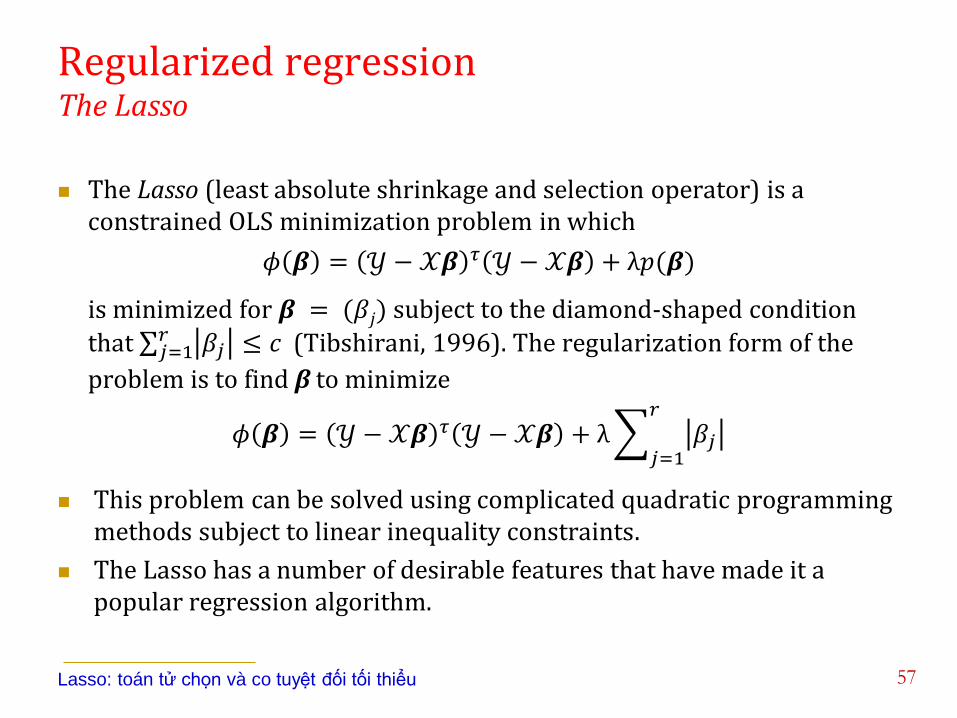
Regularized regression The Lasso
The Lasso (least absolute shrinkage and selection operator) is a constrained OLS minimization problem in which
𝜙 𝜷 = 𝒴 − 𝒳𝜷 𝜏 𝒴 − 𝒳𝜷 + λ𝑝(𝜷)
is minimized for 𝜷 = (𝛽𝑗) subject to the diamond-shaped condition
that 𝛽𝑗𝑟𝑗=1 ≤ 𝑐 (Tibshirani, 1996). The regularization form of the
problem is to find β to minimize
𝜙 𝜷 = 𝒴 − 𝒳𝜷 𝜏 𝒴 − 𝒳𝜷 + λ 𝛽𝑗
𝑟
𝑗=1
This problem can be solved using complicated quadratic programming methods subject to linear inequality constraints.
The Lasso has a number of desirable features that have made it a popular regression algorithm.
57 Lasso: toán tử chọn và co tuyệt đối tối thiểu

Regularized regression The Lasso
Like ridge regression, the Lasso is a shrinkage estimator of β, where the OLS regression coefficients are shrunk toward the origin, the value of c controlling the amount of shrinkage.
It behaves as a variable selection technique: for a given value of c, only
a subset of the coefficient estimates, 𝛽 𝑗 , will have nonzero values, and
reducing the value of c reduces the size of that subset.
58
Lasso paths for the bodyfat data.
The paths are plots of the
coefficients *β j} (left panel) and
the standardized coefficients,
*𝛽 𝑗 ∥ 𝒳𝑗 ∥ 2+ (right panel) plotted
against. The variables are added
to the regression model in the
order: 6, 3, 1, 13, 4, 12, 7, 11, 8,
2, 10, 5, 9.

Regularized regression The Garotte
A different type of penalized least-squares estimator (Breiman, 1995).
Let 𝜷 𝑜𝑙𝑠 be the OLS estimator and let W= diag{w} be a diagonal matrix with nonnegative weights w = (wj) along the diagonal. The problem is to find the weights w that minimize
𝜙 𝒘 = (𝒴 − 𝒳𝐖𝜷 ols)τ(𝒴 − 𝒳𝐖𝜷 ols)
subject to one of the following two constraints,
1. 𝐰 ≥ 𝟎, 𝟏𝑟𝜏𝐰 = w𝑗 ≤ 𝑐𝑟
𝑗=1 (nonnegative garotte, thắt cổ)
2. 𝐰𝛕𝐰 = w𝑖2 ≤ 𝑐𝑟
𝑗=1 (garotte)
As c is decreased, more of the wj become 0 (thus eliminating those particular variables from the regression function), while the nonzero
𝛽 ols,j shrink toward 0.
59

Outline
1. Introduction
2. The Regression Function and Least Squares
3. Prediction Accuracy and Model Assessment
4. Estimating Predictor Error
5. Other Issues
6. Multivariate Regression
60

Multivariate regression
Multivariate regression has s output variables 𝒀 = (𝑌1,· · · , 𝑌𝑠)𝜏, each
of whose behavior may be influenced by exactly the same set of inputs 𝑿 = (𝑋1,· · ·, 𝑋𝑟)
𝜏 .
Not only are the components of X correlated with each other, but in multivariate regression, the components of Y are also correlated with each other (and with the components of X).
Interested in estimating the regression relationship between Y and X, taking into account the various dependencies between the r-vector X and the s-vector Y and the dependencies within X and within Y.
61


