Model-based classification of radar images - Information...

1842 IEEE TRANSACTIONS ON INFORMATION THEORY, VOL. 46, NO. 5, AUGUST 2000

Model-Based Classification of Radar ImagesHung-Chih Chiang, Randolph L. Moses, Senior Member, IEEE, and Lee C. Potter, Senior Member, IEEE

Abstract—A Bayesian approach is presented for model-basedclassification of images with application to synthetic-apertureradar. Posterior probabilities are computed for candidate hy-potheses using physical features estimated from sensor data alongwith features predicted from these hypotheses. The likelihoodscoring allows propagation of uncertainty arising in both thesensor data and object models. The Bayesian classification, in-cluding the determination of a correspondence between unorderedrandom features, is shown to be tractable, yielding a classificationalgorithm, a method for estimating error rates, and a tool forevaluating performance sensitivity. The radar image features usedfor classification are point locations with an associated vector ofphysical attributes; the attributed features are adopted from aparametric model of high-frequency radar scattering. With theemergence of wideband sensor technology, these physical featuresexpand interpretation of radar imagery to access the frequency-and aspect-dependent scattering information carried in the imagephase.

Index Terms—Model-based classification, parametric modeling,point correspondence, radar image analysis.

I. INTRODUCTION

SYNTHETIC-aperture radar (SAR) provides all-weather,day-or-night remote sensing for mapping, search-and-

rescue, mine detection, and target recognition [1]. SAR dataprocessing entails forming an image from measured radarbackscatter returns, followed by processing to detect and rec-ognize targets from the formed image. Current SAR processingpractice decouples the image formation from the decision taskfor which the imagery is ultimately intended.

In this paper, a Bayesian-model-based imaging and decisionapproach is presented for classification of radar images. Theapproach provides a structured, implementable, scalable meansfor managing complexity of the hypothesis set and bypassingthe complexity of joint distributions on image pixels. Model-based classification, or pattern matching, combines uncertaintyin both the object class models and the sensor data to com-pute posterior probabilities of hypotheses. The Bayesian for-malism allows clear and explicit disclosure of all assumptions.The pattern matching permits tractable performance estimationand provides robustness against environments previously notmeasured, and hence not available for construction of imagetemplates.

Manuscript received September 1, 1999; revised April 6, 2000. This work wassupported by the U.S. Air Force Materiel Command under Contract F33615-97-1020.

H.-C. Chiang was with the Department of Electrical Engineering, The OhioState University, Columbus, OH 43210 USA. He is now with Etrend Electronics,Inc., Kaohsiung, Taiwan 80778, R.O.C. (e-mail: [email protected]).

R. L. Moses and L. C. Potter are with the Department of ElectricalEngineering, The Ohio State University, Columbus, OH 43210 USA (e-mail:[email protected]; [email protected]).

Communicated by J. A. O’Sullivan, Guest Editor.Publisher Item Identifier S 0018-9448(00)06070-3.

A. Problem Complexity

Classification of radar images, like many image inferencetasks, is characterized by a complex hypothesis space. The hy-pothesis set consists of classes, or objects; typical cases are

. The complexity arises in that each object may beobserved in a variety of poses, configurations, articulations, andenvironments, thereby resulting in an intractable density func-tion for the radar image conditioned solely on the object class.To manage the complexity, object classes are each expressed asa mixture density of subclasses. Each subclass is defined by adeterministic description of object pose, configuration, articu-lation, occlusion, sensor orientation, etc. Additional variabilitywithin subclasses is modeled stochastically to account for ob-ject differences due, for example, to manufacturing variationsor wear. The number of enumerated subclasses explodes expo-nentially; a typical application might dictate states for eachhypothesis class [2]. Moreover, an application may dictate thatmany more than decision classes be formed by defining setsof individual subclasses, ; e.g., the configuration of an ob-ject may be an important distinguishing characteristic.

Likewise, the classification of radar images is characterizedby a high-dimensional observation space defying a directrandom model. The observation, a collection of pixels, isa vector in . A typical case is a -by- array ofcomplex-valued pixels, yielding . A joint density onthe pixel values, when conditioned on a hypothesis ,is non-Gaussian and may be multimodal [7]. For example, asimple Gaussian uncertainty on the location of a scatteringmechanism leads to non-Gaussian image pixel uncertainties.Further, pixel values exhibit strong correlation due to thecoherent combination of scattered energy from an object’sconstituent parts. Multiple reflections or large conductingsurfaces can result in large distances between correlated pixels,and hence seemingly arbitrary correlation matrices.

B. Model-Based Classification

To proceed when confronting a large hypothesis space andcomplex image density functions, we adopt a model-based clas-sification approach. First, a physically based feature set providesa simple, constructive alternative to joint densities on pixels forexpressing uncertainty in the target and the sensor. The extrac-tion of features is performed by statistical estimation using thephysics-based parametric model of sensor data and specifica-tion of the image formation procedure. Second, a coarse-to-finestaged classification strategy is used to efficiently search the hy-pothesis space. Third, the sensor data model is combined withobject models to predict features conditioned on a hypothesis.The on-line prediction of features eliminates the need for a pro-hibitively large catalog of image templates.

0018–9448/00$10.00 © 2000 IEEE

CHIANG et al.: MODEL-BASED CLASSIFICATION OF RADAR IMAGES 1843

Fig. 1. A model-based approach to classification.

The model-based approach is depicted in Fig. 1. A state ofnature is characterized by the hypothesis of an object classwhich is further specified by one of finitely many subclasses

. The SAR measurement resulting from a sensor and animage-formation algorithm provides an image. Along the leftbranch in the figure, a Feature Extraction stage serves to com-press the image and assign uncertainties to features. For SARimaging, a sensor data model derived from high-frequency ap-proximation to scattering physics provides a parametric familyof densities for estimating features. Parameters are estimatedfrom imagery and used as low-dimensional surrogates for suffi-cient statistics; each feature is a location together with a vectorof attributes. The feature uncertainty is given as a density func-tion and acknowledges the sensitivity of parameter es-timates to noisy sensor data given the image data.

Along the right branch in the figure, complexity of the hy-pothesis space is addressed in a coarse-to-fine approach. AnIndex stage provides a list of candidate subclass hypotheses

based on a coarse partitioning of the hypothesis space.Evaluation of the candidate hypotheses then proceeds using amodel for the observations. A Feature Prediction stage com-putes a predicted feature set by combining the sensor data modelfrom the Feature Extraction stage and a computer-aided design(CAD) representation of a hypothesis . The feature set hasan associated uncertainty, acknowledging error in the modelingand variation among objects in the subclass. The uncertainty isexpressed as a density . Importantly, the use of phys-ically motivated features facilitates compatibility of extractedand predicted feature sets.

Finally, the predicted and extracted feature sets are combinedin a Match stage to compute a posterior probability of a can-didate hypothesis . The top hypotheses, and their like-lihoods, are reported as the output of the classification system.Computation of the likelihood scores requires a correspondencebetween the unordered lists of extracted and predicted featuresand an integration over feature uncertainty. Further, the likeli-

hood must incorporate the possibilities of missing or spuriousfeatures in the predicted or extracted feature lists. The matchingtask can be viewed as a probablistic graph match of fully con-nected, attributed graphs with deletions and insertions of nodes.

C. Contributions and Organization

This paper presents a Bayesian formalism for model-basedclassification. We demonstrate that the resulting hypothesistesting algorithm, including the feature correspondence, istractable, even for problem sizes encountered in SAR targetrecognition. In addition, the paper adopts a physics-basedmodel for extracting features from SAR images; the featuresuse the phase in complex-valued SAR images to infer thefrequency- and aspect-dependent scattering behavior of ob-jects. Recent advances in technology yield sensor bandwidthsexceeding 20% of the center frequency; for such systems, theproposed feature sets provide much greater information thandoes processing motivated by a narrowband point-scatteringmodel.

Detailed construction of the Index and Feature Predictionstages is not considered here; these stages are discussed in [3]and [7]. An adaptive refinement of the candidate hypothesislist from the Index stage is considered in [6]. Moreover, a Fea-ture Prediction stage that faithfully simulates frequency- and as-pect-dependent scattering behavior is currently under develop-ment [7].

The paper is organized as follows. In Section II we present aparametric model for radar sensor data, as required in the Fea-ture Extraction and Feature Prediction stages. Maximum-like-lihood estimation of parameters from images computed usingsensor data is discussed; also, parameter uncertainty, the defi-nition of image resolution, and the Fisher information in imagephase are addressed. Section III presents a Bayesian computa-tion of a hypothesis likelihood given sets of extracted and pre-dicted features. In particular, the problem of determining a fea-ture correspondence is addressed.

In Section IV, synthetic classification results are computedusing class means estimated from a measured set of-bandradar images for ten objects. The simulation results illustratefour points: 1) the Bayes approach to model-based classifica-tion, including feature correspondence, is tractable; 2) classifi-cation using the Bayes classifier permits estimation of the op-timal error rate, given the assumed priors and feature uncertain-ties; 3) classification using the Bayes classifier allows designersto explore the performance effects of sensor parameters, such asbandwidth; and iv) classification using the Bayes classifier pro-vides a simulation tool to investigate sensitivity of the estimatederror rate to the assumed priors and feature uncertainties.

II. A PHYSICAL MODEL FOR SENSOR DATA AND

FEATURE EXTRACTION

In this section we address the problem of feature extraction.We adopt a parametric model describing the sensor data, de-velop a feature estimation algorithm, and discuss feature uncer-tainty both for extraction and feature prediction. The model weemploy is based on high-frequency approximation of electro-magnetic scattering [9], [11] and represents the object of interest


as a set of scattering centers. The scattering centers are describedby attributes that characterize the scattering center geometry andorientation. The attributed scattering centers are used as featuresfor both the prediction and extraction stages in Fig. 1. The scat-tering model provides a method of constructing and succinctlyrepresenting hypotheses from CAD representations of class ob-jects. Additionally, the model allows feature extraction to be castas a parameter estimation problem.

For a Bayesian classifier, uncertainty must be characterizedfor both predicted and extracted feature sets. Because the pro-posed features relate directly to physical components in a CADrepresentation, uncertainty in predicted features can be esti-mated from uncertainty in the CAD model. This is an importantadvantage of using a physics-based model; other parametricmodels could be used to represent the measured data, but unlessthe model parameters relate to scattering physics, it is verydifficult to model the prediction uncertainty in Fig.1. In addition, a parameter-estimation formulation of featureextraction provides means for describing feature uncertainty

and for bounding it with the Cramér–Rao bound.The model-based interpretation of images permits an infor-

mation-theoretic view of SAR imaging. We consider two im-plications of this viewpoint. First, we define SAR image reso-lution in terms of uncertainty in estimated parameters. Second,we consider performance degradation when incomplete data areavailable. Incomplete data availability results in higher featureuncertainty as measured by relative information; as an example,we consider the increase in uncertainty that results from thecommon practice of discarding the phase of the SAR image.

A. A Parametric Model for Object Scattering

Most feature extraction models used with SAR rely onprocessing of the magnitude image. For example, featuresused in the MSTAR program are peaks (local maxima of theSAR magnitude image) and ridges obtained from directionalderivatives of the SAR magnitude image [3]. When the com-plex-valued SAR image is used, the point-scattering model ismost commonly employed; in this model, the backscattered am-plitude is assumed to be independent of frequency and aspect.The point-scattering assumption leads to a two-dimensionalharmonic scattering model, and parameter estimation becomesa two-dimensional harmonic retrieval problem [4], [5]. Onedrawback of peak and point scattering models is that a singlescattering object, such as a dihedral, is modeled as severalpeaks or point scatterers; in this case, the correlated uncertaintyin the estimated parameters is difficult to model. Similarly, therelationship of ridge features to scattering geometry is not wellunderstood, and feature uncertainty is hard to predict.

In this paper we adopt the physical radar scattering modelfrom Gerryet al. [9], which assumes a data collection scenarioconsistent with SAR imaging. A reference point is defined, andthe radar trajectory is required to be coplanar with the refer-ence point. This plane, the imaging plane, is labeled using an

Cartesian coordinate system with origin at the referencepoint. The radar position is then described by an angledefinedcounterclockwise from the direction. Far-zone backscatter isassumed, and therefore planewave incidence is obtained on il-luminated objects.

From the geometric theory of diffraction (GTD) [12], [13], ifthe wavelength of the incident excitation is small relative to theobject extent, then the backscattered field from an object con-sists of contributions from electrically isolated scattering cen-ters. The backscattered field of an individual scattering center isdescribed as a function of frequencyand aspect angle, andthe total scattered field from a target is then modeled as the sumof these individual scatterers [9]

(1)

In (1), is the center frequency of the radar bandwidth, andis the speed of propagation. Each ofscattering centers is

characterized by seven attributes: denotes the scatteringcenter location projected to the -plane, is a relativeamplitude, is the scattering center length, its orientationangle, characterizes frequency dependence of the scatteringcenter, and models the mild aspect dependence of scatteringcenter cross-section (for example, the projected cross-sectionalarea of a trihedral changes slightly with aspect angle). The scat-tering model is described by the parameter set ,where each vector is the col-lection of the seven parameters, or attributes, defining each scat-tering center.

The frequency and aspect dependence of the scattering cen-ters is an important distinction of this model and permits de-scription of a rich variety of scattering primitives. The frequencydependence relates directly to the curvature of the scatteringobject and is parameterized by , which takes on integer orhalf-integer values. For example, describes flat surfacescattering, describes scattering from singly curvedsurfaces, and indicates scattering from doubly curvedsurfaces or edges. Values ofless than zero describe diffrac-tion mechanisms, such as edges and tips. In addition, the sincaspect dependence in (1) reveals the effective lengthof thescattering primitive. Many scattering geometries, such as dihe-drals, corner reflectors, and cylinders, are distinguishable bytheir parameters [9], as shown in Fig. 2. Point scatteringis a special case of the model in (1) for .

The model in (1) is based on GTD and physical optics ap-proximations for scattering behavior and, while parsimonious,is able to describe a large class of scatterers. Scattering objectsseparated by approximately two or more wavelengths are dis-tinguishable [10]. Physical behaviors not well modeled by (1)for small include creeping waves and cavity scattering [9].

B. Parameter Estimation

Next, we describe an approximate maximum-likelihood tech-nique for extracting the model parameters in (1) from measuredsensor data. The measured data is modeled as

(2)


Fig. 2. Canonical scattering geometries that are distinguishable from(�;L)pairs in the scattering model.

where is a noise term that represents the modeling error(background clutter, sensor noise, model mismatch, incompletemotion compensation, antenna calibration errors, etc.) and canbe modeled as a zero-mean, Gaussian noise process with knowncovariance.

The measured data is often transformed into the image do-main as an array of complex-valued pixels. The transforma-tion comprises equalization (to compensate for nonideal sensorcharacteristics), windowing, zero padding, and discrete Fouriertransformation. The transformation can be represented by thelinear operator ; thus

(3)

for a finite array of sample points . We see that is azero-mean Gaussian noise process with known covariance. Thefeature-extraction problem is thus one of estimating the param-eter vector from the measurement .

R. A. Fisher’s pioneering work laid a foundation forparametric modeling as a method of data compression, andestablished maximum-likelihood procedures for estimationof the unknown parameters [8]. Since are Gaussianmeasurements, the parameter vectorwhich maximizes thelikelihood function is found as

(4)

(5)

where and are vectors obtained by stacking thecolumns of and respectively;

, and denotes Moore–Penrose pseudoinverse.Furthermore, this estimator is robust to model mismatch [15].Equation (4) is a nonlinear least squares minimization problem.

We make use of the fact that scattering center responses arelocalized in the image domain to develop a computationally sim-pler approximate maximum-likelihood estimator for[14]. Theminimization in (4) is decomposed into smaller estimation prob-lems. We partition the image into disjoint regions of highenergy and a remainder region . Defining as the projec-tion onto region , we have

(6)

where is a vector containing the parameters for scattering cen-ters in region and is a constant independent of. Since

the number of pixels in is much less than the total numberof image pixels in and the form a partition of , the in-dividual minimization problems in (6) are decoupled and havemany fewer unknowns than the minimization problem in (5).The weighted least squares estimator is tractable and providesnearly efficient parameter estimates for data satisfying the scat-tering model in (1) with colored Gaussian noise on image pixels[14].

An additional advantage of the approximate maximum-like-lihood (ML) algorithm is its robustness to the assumed noisemodel. The assumption of correlated Gaussian noise across theentire image is not very accurate for scenes where clutter ispresent in the form of trees, power lines, etc. However, this as-sumption is much better over small image regions that primarilycontain target-scattering centers. Image segmentation also fa-cilitates model order selection, which is implemented using theminimum description length principle.

As an illustration of the approximate ML estimation, Fig. 3shows the results of feature extraction on a measured SARimage from the MSTAR Public Targets dataset [26]. For

, the algorithm models 96.5% of the energy in theimage chip shown. In addition, the T-72 tank barrel segment ismodeled as a single scattering center whose length is modeledwithin 10 cm of the actual 1.37-m length. In comparison,peak-based scattering center extraction methods model thissegment as three peaks spaced along the barrel. Executiontime for extraction of 30 scattering features using unoptimizedMatlab code on a 450-MHz Pentium processor is approximately140 s using (5) and approximately 50 s if a suboptimal butcomputationally efficient estimator is employed.

C. Parameter Uncertainty

Use of estimated model parameters for Bayesian hypothesistesting requires that an uncertainty be associated with each es-timate. The inverse of Fisher information is used to predict theerror covariance of the approximate maximum-likelihood esti-mation algorithm in (6).

The Cramér–Rao lower bound is derived in [9] and providesan algorithm-independent lower bound on the error variance forunbiased estimates of the model parameters. The derivation as-sumes the data model in (3). For any choice of model param-eters, the covariance bound is computed by inversion of theFisher information matrix [16]

(7)

where is density on the sensor dataconditioned on theparameter .

D. Image Resolution

As noted in [17], “a universally acceptable definition of res-olution as a performance measure is elusive.” In SAR, imageresolution is typically reported as the width of a point-spreadfunction. This definition is a Rayleigh resolution and is deter-mined by sensor bandwidth, range of viewing angles, and de-gree of sidelobe suppression in image formation. In contrast,for model-based interpretation of SAR imagery we define reso-


Fig. 3. Measured SAR Image of T-72 Tank (top) and reconstruction from estimated parameters (bottom). Images are in decibel magnitude with a total range of40 dB.

lution in terms of a bound on the uncertainty in estimated param-eters. Prior knowledge of the scattering behavior, as encoded in(1), results in an uncertainty-based resolution that is often muchfiner than the Rayleigh resolution. For example, consider ap-plication of feature uncertainty to the classical notion of sepa-rating closely spaced point sources, i.e., in (1).For a given signal-to-noise ratio (SNR) of a single-point scat-terer (SNR per mode), let the resolution be defined as the min-imum distance between two equal amplitude scattering centersresulting in nonoverlapping 95% confidence regions for the es-timated locations [9], [18].

Adopting this definition, resolution versus SNR per mode isshown in Fig. 4 for a SAR with Rayleigh resolution of 30 cm.The resolution depends on the orientation of the two point scat-terers. The dashed line shows resolution for point scatterers sep-arated an equal distance in both down range and cross range (i.e.,aligned 45 to the aperture). The solid line and the dash–dotline show resolution for two point scatterers aligned paralleland orthogonal to the aperture, respectively. For an SNR permode of 5 dB and 500-MHz bandwidth, the limit of resolutionachievable by model-based scattering analysis is approximatelyone-half the Rayleigh resolution; model-based resolution is lim-ited by sensor bandwidth and SNR, which includes mismatchfrom the model in (3).

In the figure, we report signal-to-noise (SNR) values usingthe ratio of signal energy to noise energy computed for the fre-quency-aspect domain samples. Alternatively, SNR may be in-terpreted in the image space as a difference between peak signallevel and clutter floor. However, this image space definition ofSNR varies depending on the specific values of the parametervector describing the scattering center.

E. Magnitude-Only Fourier Data

The parameter uncertainty definition of resolution can be di-rectly applied to image reconstruction from incomplete data;for example, in SAR image formation a common practice is todiscard image phase. In this case, the estimation of be-comes reconstruction from magnitude-only Fourier data. TheFisher information can be computed for the sampledmagnitude of the image data, using (1) and knowledge of boththe sensor transfer function and the image formation operator.The relative information [19] is the ratio of Fisher matrices

and quantifies the loss of information incurred bydiscarding the image phase. Likewise, the increase in variancein any parameter estimate can be predicted, for efficient estima-tors, using the Cramér–Rao bounds.

For example, for 10 GHz, 3-GHz bandwidth, and10-dB SNR, the Cramér–Rao bound on standard deviation in


Fig. 4. Resolution versus SNR for three different orientations of two point scatterers;! =(2�) =10 GHz, and bandwidth is 500 MHz.

estimation error for is using a magnitude image. Incontrast, estimation of from the complex-valued image resultsin . Thus use of complex-valued imagery allows infer-ence of the frequency-dependent scattering behavior, whereasuse of magnitude-only imagery does not.

III. H YPOTHESISTESTING

A. Problem Statement

In this section we derive the Bayes match function used forclassification from feature vectors. At the input to the classifierstage, we have a given region of interest (a SAR image chip),along with a set of candidate target hy-potheses and their prior probabilities . Each hypothesiscontains both target class and subclass information; the setmay contain all possible hypotheses but typically contains a re-duced set as generated from an earlier Index stage as depicted inFig. 1. From the image chip we extract a feature vector, andfrom each candidate hypothesis we generate a predictedfeature vector , where

(8)

and where and are the number of predicted and extractedfeatures, respectively. Each feature and is an orderedvector of feature attributes; for example, these attributes can be

parameters from the model in (1). However,the features themselves are unordered. In addition, there is un-certainty in both the predicted and extracted features.

There are two hypothesis testing goals that may be of interest.First, we may wish to classify the extracted feature vectoras ameasurement of one of the class hypotheses. Second, we maywish to classify as one of the class–subclass hypotheses in

the set . For both cases, we adopt a maximuma posterioriprobability (MAP) rule; thus we must find the posterior likeli-hoods

(9)

If our goal is to classify as one of the Index hypotheses(which include both class and subclass information), we choosethe hypothesis that corresponds to the maximum. If our goalis to classify as one of the class hypotheses, we form

(10)

and choose the classcorresponding to the maximum .The above formulation gives an interpretation of the Index

block in Fig. 1 as modifying the prior probabilities on theclass and subclass hypotheses. The optimal MAP classifiermaximizes or sums over all possible classes, and not justthose provided by the Index stage. The Index stage computes astatistic from the image , and essentially updatesprobabilities of hypotheses by finding posterior probabili-ties . A subset of hypotheses with sufficiently highposterior probabilities are retained for further processing. Thefinal hypothesis test involves computing ; thus thefeature-based match processing seeks to extract information in

not contained in to obtain a final classificationdecision. We see that the Index stage does not impact opti-mality in (9) provided the correct hypothesis is one of thehypotheses passed. On the other hand, from (10) we see thatthe optimal MAP rule involves summation over all subclassesin class , not just those passed by the Index stage. Thus (10) isoptimal only under the stronger condition that the likelihoods

of all subclasses not passed by the Index stage are


equal to zero. In either case, the computational reduction ofmaximizing or summing on a reduced set of subclasses oftenjustifies the deviation from optimality of the resulting classifier.

To compute the posterior likelihood in (9), we apply Bayesrule for any to obtain1

(11)

The conditioning on is used because the number of featuresin is itself a random variable, but it suffices to consider onlyvectors of length in the right-hand side of (11). Since thedenominator of (11) does not depend on hypothesis, the MAPdecision is found by maximizingover . The priors and are assumed to beknown, or are provided by the Index stage.

The determination of includes both predictionand extraction uncertainties, which are related in the followingway. Assume we have an object in the field with feature vector

. We measure that object with a sensor, and obtain a featurevector . The measured feature vector differs fromdue tonoise, sensor limitations, etc. We write this difference notion-ally as where is some extracton error describedby an uncertainty probability density function (pdf) . Inaddition, if we suppose a hypothesis, we can predict a featurevector that differs from because of electromagnetic mod-eling errors, quantization errors of the assumed object subclassstates (e.g., pose angle quantization errors), and differences be-tween the actual object in the field and the nominal object thatis modeled. We express this difference as where

is a prediction error which we describe with an uncertainty. Note that is completely determined from . To

find the conditional uncertainty of given hypothesis , wehave

(12)

where models the predict uncertainty, andmodels extract uncertainty. The computation

of is complicated by the fact that the featuresin the and vectors are unordered, so a correspondencebetween the elements of and , or equivalently betweenand , is needed.

B. Feature Correspondence

Computing the likelihood requires that weform a correspondence mapbetween extracted and predictedfeatures. The correspondence map is a nuisance parameter thatarises because an extracted feature vector is not ordered withrespect to the predicted feature vector. The correspondencealso accounts for extracted features that are not in the predictedvector (false alarms) as well as predicted features that are notextracted (missed features).

For general pattern matching applications, a predicted featuremay correspond to none, one, or several extracted features

1For notational simplicity, we drop the subscripts on the hypotheses in thesequel, and consider a generalH 2 H.

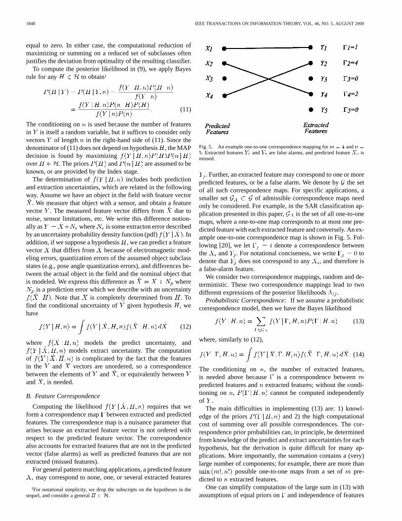
Fig. 5. An example one-to-one correspondence mapping form = 4 andn =5. Extracted featuresY andY are false alarms, and predicted featureX ismissed.

. Further, an extracted feature may correspond to one or morepredicted features, or be a false alarm. We denote bythe setof all such correspondence maps. For specific applications, asmaller set of admissible correspondence maps needonly be considered. For example, in the SAR classification ap-plication presented in this paper, is the set of all one-to-onemaps, where a one-to-one map corresponds to at most one pre-dicted feature with each extracted feature and conversely. An ex-ample one-to-one correspondence map is shown in Fig. 5. Fol-lowing [20], we let denote a correspondence betweenthe and . For notational conciseness, we write todenote that does not correspond to any , and therefore isa false-alarm feature.

We consider two correspondence mappings, random and de-terministic. These two correspondence mappings lead to twodifferent expressions of the posterior likelihoods.

Probabilistic Correspondence:If we assume a probabilisticcorrespondence model, then we have the Bayes likelihood

(13)

where, similarly to (12),

(14)

The conditioning on , the number of extracted features,is needed above becauseis a correspondence betweenpredicted features andextracted features; without the condi-tioning on , cannot be computed independentlyof .

The main difficulties in implementing (13) are: 1) knowl-edge of the priors and 2) the high computationalcost of summing over all possible correspondences. The cor-respondence prior probabilities can, in principle, be determinedfrom knowledge of the predict and extract uncertainties for eachhypothesis, but the derivation is quite difficult for many ap-plications. More importantly, the summation contains a (very)large number of components; for example, there are more than

possible one-to-one maps from a set ofpre-dicted to extracted features.

One can simplify computation of the large sum in (13) withassumptions of equal priors onand independence of features


[20], [21]. If the priors are not equal or the features are not in-dependent, then the resulting classifier will be suboptimal. It isdifficult to predict the performance loss due to mismatch be-tween the assumed and actual priors.

Deterministic Unknown Correspondence:If we assume thecorrespondence is deterministic but unknown, then it becomesa nuisance parameter in the classification. In this case, no uni-formly most powerful test exists. We thus resort to the Gener-alized Likelihood Ratio Test (GLRT) classifier, in which we es-timate , then use the estimatedto estimate the likelihoods

(15)

where is computed using (14). The GLRT ap-proach in (15) avoids the summation in (13), but requires asearch for the best correspondence. Graph matching algorithms[22] can be used to simplify this search.

Discussion: The GLRT estimate of the conditional likeli-hood is a good estimate of the Bayes likelihood if the “best” cor-respondence term (15) dominates the sum in (13). This happensin the SAR classification problem, for example, when the fea-ture uncertainties are small compared to their feature distances;for example, the match likelihood when corresponding two fea-tures with widely differing locations is negligibly smallcompared to the likelihood found from associating all pairs offeatures with similar locations. The presence of additionalscattering attributes helps increase the feature distances even forscattering features that have similar locations; for example, twophysically close scattering centers with differentand pa-rameters have lower likelihood of an incorrect match pairingthan they would if match scores were based only on scattererlocation and amplitude.

For the SAR classification application, we adopt both a one-to-one map and a GLRT classifier. The one-to-one map makesphysical sense: an extracted scattering center corresponds toat most one predicted scattering center, and conversely. TheGLRT classifier assumes a deterministic but unknown corre-spondence map, and avoids summation over a large set of pos-sible correspondence maps. The probabilistic map assumptionfor this model is considered in [21]. In addition, [20] considersother classifiers derived for SAR features using only locationattributes.

C. Conditional Feature Likelihood

To implement either (13) or (15), one must have available amodel for . In this section we develop a modelbased on [20] that applies to SAR scattering center features.

We assume the are conditionally independent given,and that are conditionally independent given, , and .The independence of the is reasonable because the predic-tion errors of separate scattering centers are due to variations incomponents on the target that make up that scattering center,and these variations can be assumed to be unconnected. Theindependence of the is supported by the near block diag-onality of the CRB matrix for well-separated scattering cen-

ters [9]. In addition, the independence assumptions simplify theBayes matcher significantly. Thus we have

(16)

For a one-to-one correspondence, theth extracted featurecorresponds either to a particular predicted feature (say, thethone), or to a false alarm. We denote these two cases asor , respectively. Thus for a given correspondence, theremay be some predict–extract feature correspondences, somemissed predicted features (which correspond to no extractedfeature), and some false-alarm extracted features which haveno corresponding predict feature; see Fig. 5. For a given corre-spondence, let denote the number of false-alarm features.

We model the conditional feature likelihood as

false alarms

(17)

where is the detection probability of theth predicted fea-ture under hypothesis . The first term on the right-hand sidemodels the likelihood of false-alarm features, and is thepdf of feature if it corresponds to a false alarm. The secondline is the likelihood of extracted features that correspond to pre-dicted features, and the third line represents the miss probabil-ities for predicted features that have no corresponding extractfeature.

D. Implementation of the Correspondence Search

The GLRT hypothesis selection rule in (15) involves findingthe correspondencethat maximizes in (17) foreach candidate hypothesis . In general, the search iscomputationally intensive, but for some cases can be imple-mented efficiently. Specifically, in the case that

false alarms (18)

for some constantsand , the search can be efficiently imple-mented in operations using the Hungarian algo-rithm [22].

We briefly summarize the implementation of the Hungarianalgorithm for this problem.2 From (17) and (18) we have

(19)

2The authors thank William Irving for noting the application of the Hungarianalgorithm to this search problem.


Fig. 6. The cost matrix for the one-to-one matcher in (17). Here,c =

� log[P (H)f(Y j� = i; H)], F = � log[�f (Y )], and M =� log[1�P (H)].

We insert the elements of the above equation for all possibleand into an array, as shown in Fig. 6.Then the minimum of (19) over all one-to-one maps reduces tothe problem of selecting exactly one element from each row andcolumn of the array such that the sum of the selected entries isminimized. The resulting solution also gives the optimal corre-spondence. Specifically, if is selected, then predicted feature

corresponds to extracted feature; if is selected, thenis a false-alarm feature; if is selected, then is not present(missed) in the extracted features.

The search is equivalent to finding a permutation of the costmatrix that minimizes its trace. Such a permutation is found effi-ciently using the Hungarian algorithm [22]. A related algorithm[23] can also find the permutations that give the smallesttrace values, which is useful if the “best”correspondences areof interest.

As an alternative, geometric hashing [24], [25] can be used toefficiently search a set of candidate hypotheses for the highestlikelihood match. Hashing methods precompute informationabout patterns of features in a hash table that later can be effi-ciently searched to vote for hypotheses that are close matches.On the other hand, hashing requires the formation of a largetable, containing entries for every hypothesis ; this tablecan be prohibitively large for high-dimensional classificationapplications.

IV. BAYES CLASSIFICATION EXAMPLE

In this section we present an example of feature-based clas-sification using SAR scattering center attributes. We use syn-thetic feature vector means based on measured SAR imageryand an assumed feature perturbation model. We select targetclasses, feature sets, feature attribute uncertainties, and priorsto be representative of a realistic-band SAR target-recog-nition problem. The synthetic data results serve to emphasize,by example, that the Bayes classifier is tractable for problemsizes encountered in SAR target recognition given the assump-tion of conditionally independent features in Section III-C. Theproposed technique permits estimation of the optimal error rategiven a set of assumed priors and feature uncertainties. In addi-tion, we demonstrate by example that the Bayes classifier canbe used to explore the performance effects of sensor parame-ters. Finally, the Bayes classifier can be used as a simulation tool

to investigate sensitivity of the estimated error rate to errors inassumed priors and feature attribute uncertainty. Accurate pre-diction of absolute classification performance would require anelectromagnetic prediction module as in Fig. 1 and extractionuncertainties empirically verified from ground truth; neither ispresently available.

We generate class means using a combination of syntheticgeneration and feature extraction from SAR imagery. We syn-thesize 2747 class mean features for ten composite target classesin the MSTAR Public Targets dataset [26]. The data set contains

-band image chips with pixels and 1 ft 1 ft reso-lution SAR data chips of 10 targets at 17depression angle. Foreach target, approximately 270 images are available coveringthe full 360 aspect angles, for a total of 2747 images. Down-range and cross-range locations and amplitudes of scatteringcenters are synthesized from local maxima on the image chips.The targets are the 2S1, BMP-2, BRDM-2, BTR-70, BTR-60,D-7, T-62, T-72, ZIL-131, and ZSU-23-4. Examples of the SARimage chips are shown in Fig. 7. From each image we extract lo-cations and amplitudes of scattering centers from local maximain the SAR image. The and parameters are not provided bycurrent prediction modules, so are generated synthetically. The

attribute for each feature is generated as .The Gaussian approximation to a discrete variable is used toavoid the combinatorial number of likelihood evaluations for allpossible choices from prediction and extraction; experimentsverify that the Gaussian approximation gives very similar resultsat lower computational cost [21]. The length parameter is quan-tized to 1 bit ( or ), and the nominal values of thelength attribute are generated using a Bernoulli random variablewith . We quantize because existing electro-magnetic prediction codes do not provide; further, predictionuncertainty is unknown, so we choose to adopt only coarse un-certainty assumptions in the simulation. Theand parame-ters in (1) are not used in the experiments because no strongevidence exists that these parameters can be predicted and ex-tracted at 1-ft SAR resolution with sufficiently low uncertaintyto substantially improve classification performance; nonethe-less, these two parameters are retained in (1) both for reducedbias and for application to higher resolution SAR imagery. Forexample, using 2-in resolution SAR imagery at-band, poseangle can be estimated to an accuracy that is a small fraction ofthe 20 phase history angle used in the image formation.

Prediction and extraction feature uncertainties are neededin the Bayes classifier. We evaluatein (17) as follows. Recall each is a feature vector

where the are the individual featureattributes , and from the model in (1)(or a subset of these). For simplicity, we assume the uncer-tainties of the feature attributes are independent; experimentsusing dependent attribute uncertainties are presented in [21].For independent attributes

(20)

where denotes an index on the feature attributes. We furthermodel each attribute in an extracted feature that corre-sponds to predicted feature with a conditional likelihood


Fig. 7. Examples of the MSTAR SAR image chips used in the Bayesclassificaion example. Four T-72 (left) and BMP-2 (right) images are shown.

as follows. If corresponds to, , ,or , the conditional likelihood is assumed to be Gaussian

(21)

We assume a similar predict uncertainty for each attribute

(22)

Thus from (14), (21), and (22) we have

(23)

which gives the needed terms in (20). Similarly, for a discreteattribute (the quantized length) the likelihood is a weightedsum

(24)

and is thus described by probability mass functions on the pre-dicted features along with predict and extract confusion ma-trices.

From (23) and (24) we see that only the sum of prediction andextraction uncertainties is needed. Table I lists the uncertaintyvalues used in the simulations. We assume no prediction uncer-tainty in or , and log-normal uncertainty in . The totallocation uncertainty is assumed to have a standard deviation ofone Rayleigh resolution for both and . In addition, Table IIspecifies the false-alarm pdf .

We emulate the Index stage as follows. For each of the 2747target image chips, we find the five image chips in each of the tentarget classes that have the highest correlation. The target classesand poses (pose is in this case azimuth angle) corresponding tothese 50 image chips form the initial hypothesis list generatedby the Index stage. For each class mean vector, we generate apredict feature vector for each of the 50 hypotheses from theIndex stage by randomly perturbing the mean vector using thepredict uncertainty model above. We similarly generate an ex-tracted feature vector from the mean vector. The extracted fea-ture vector assumes each scattering center has a probability ofdetection of , so not all scattering centers are present inthe extracted feature vector. We also add clutter scattering cen-ters to the extract feature vector. We then compute the GLRT hy-pothesis test using (11), (15), and (17), assuming equally likelypriors constanton the 50 Index hypotheses.We use the Hungarian algorithm to search for the best corre-spondence map, using in (18). We record the targetclass corresponding to the one of the 50 hypotheses with thehighest likelihood score. We repeat this experiment ten timesfor each class mean vector; this gives a total of 27 470 classifica-tions from 27 470 50 matches. For each candidate hypothesis,computation of the correspondence is , where is thenumber of predicted features. Execution times for the 50 like-lihood computations average 4.6 s using unoptimized Matlabcode on a 333-MHz Pentium processor.

Table III presents the results of the above experiment for aSAR Rayleigh resolution of 1 ft, using the uncertainty values inTable I. We summarize the overall performance as an averageprobability of correct classification , which is 86.8% for thiscase.

Fig. 8 presents probability of correct classification resultsas a function of both the number of feature attributes and thesystem bandwidth. First we compare the use of location featureswith location features coupled with other attributes. The ampli-tude attribute provides only modest improvement (1–2 dB) inthe probability of error, due to its relatively high uncertainty.The addition of the frequency dependence and length attributesprovides more significant improvement in classification perfor-mance, especially for the higher resolutions considered. Theamount of improvement depends critically on the assumed at-tribute uncertainty and its correlation with other attributes.

Fig. 8 also presents results of an experiment in which wepredict classification performance as a radar system parameter,namely, Rayleigh resolution, changes. The bandwidths andintegration angles correspond approximately to SAR imageRayleigh resolutions of 2, 1, 1/2, and 1/4 ft. We assume de-creasing uncertainty in the location, frequency dependence, andlength attributes as Rayleigh resolution becomes finer, as shownin Table I. From Fig. 8 we see that classification performanceimproves significantly as radar bandwidth and integration angleincrease. Specifically, the error probability decreases byabout 15 dB as the SAR Rayleigh resolution improves from 2 ftto 1/4 ft. Here we see a clear benefit of increased bandwidthbecause it results in decreased feature uncertainty.

Fig. 9 shows the effect on classification performance whenthe assumed uncertainty model in the Bayes classifier is in error.In this experiment we set the location uncertainty standard de-


TABLE ISUM OF PREDICTION AND EXTRACTION FEATURE ATTRIBUTE UNCERTAINTIES USED IN THE BAYES CLASSIFIER EXAMPLE

TABLE IIFALSE-ALARM pdf f (Y ) USED IN THE BAYES CLASSIFIER EXAMPLE

TABLE IIIONE-TO-ONE CLASSIFICATION RESULTS USING FIVE FEATURE ATTRIBUTES. THE ijTH ENTRY GIVES THE NUMBER OF TIMES THE OBJECTWAS

CLASSIFIED AS OBJECTj GIVEN THAT OBJECTi IS THE TRUE OBJECT. OVERALL P = 86.8%

viation to 0.5, 1, and 2 times the correct location uncertainty;the other attributes use the correct uncertainty models. Here,

. We see the correct classification rate drops by10% –20% as a result of the mismatch, and that a greater per-formance loss occurs when the model-based classifier assumestoo low an uncertatinty.

V. CONCLUSION

We have presented a model-based framework for image pro-cessing when the processing goal is object classification. TheBayesian formalism allows clear and explicit disclosure of allassumptions, in contrast toad hocclassification procedures.


Fig. 8. Classification performance as a function of number of feature attributes and radar bandwidth. The top graph shows average probability of correctclassification(P ); the bottom graph shows the same data plotted as average probability of error(1� P ) in decibels.

Fig. 9. Classification performance using correct (center) and erroneous location uncertainties in the Bayes classifier. The left (right) bars assume 0.5 (2) timesthe true location uncertainty. The top graph shows average probability of correct classification(P ); the bottom graph shows the same data plotted as averageprobability of error(1 � P ) in decibels.


Moreover, we demonstrated that the Bayes approach, includingthe associated correspondence problem, is tractable and leads toimplementable algorithms.

We have presented the Bayes approach to model-basedclassification in the application context of synthetic apertureradar (SAR) imagery. By modeling electromagnetic scatteringbehavior and estimating physically meaningful parametersfrom complex-valued imagery, we computed features asstatistics for use in hypothesis testing. For radar systems witha significant fractional bandwidth, the features provide richerinformation than local peaks in magnitude imagery.

A complete empirical evaluation of the proposed classifier re-quires an electromagnetic scattering code to provide predictedfeatures conditioned on a target hypothesis; at the time of thispublication, such a code is being developed by Veridian-ERIMInternational, Inc., as a hybrid combination of the ray-tracingand scattering primitive codes. Further, the efficacy of the pro-posed likelihood estimation technique requires additional em-pirical verification of the feature uncertainties adopted in Sec-tion IV; to do so requires ground truth that is not currently avail-able, but would be provided by the scattering prediction codeunder development.

The implementable Bayes classifier allows estimation of op-timal error rates, given assumed priors and feature uncertainties,and the simulation of performance sensitivity to assumed priors,to assumed feature uncertainties, and to sensor characteristics.

ACKNOWLEDGMENT

The authors wish to thank William Irving and Edmund Zelniofor informative discussions on correspondences of random fea-ture vectors, staged hypothesis evaluation, and application tomicrowave radar images.

REFERENCES

[1] J. C. Curlander and R. N. McDonough,Synthetic Aperture Radar: Sys-tems and Signal Processing. New York: Wiley, 1991.

[2] E. R. Keydel, S. W. Lee, and J. T. Moore, “MSTAR extended operatingconditions: A tutorial,” inAlgorithms for Synthetic Aperture Radar Im-agery III (Proc. SPIE), E. Zelnio and R. Douglass, Eds., no. 2757, 1996,pp. 228–242.

[3] T. W. Ryan and B. Egaas, “SAR target indexing with hierarchical dis-tance transform,” inAlgorithms for Synthetic Aperture Radar ImageryIII (Proc. SPIE), E. Zelnio and R. Douglass, Eds., no. 2757, 1996, pp.243–252.

[4] D. F. DeLong and G. R. Benitz, “Extensions of high definition imaging,”in Algorithms for Synthetic Aperture Radar Imagery II (Proc. SPIE), D.A. Giglio, Ed., no. 2487, 1995, pp. 165–180.

[5] J. Li and P. Stoica, “An adaptive filtering approach to spectral estima-tion and SAR imaging,”IEEE Trans. Signal Processing, vol. 44, pp.1469–1484, June 1996.

[6] J. Wissinger, R. Washburn, D. Morgan, C. Chong, N. Friedland, A. Now-icki, and R. Fung, “Search algorithms for model-based SAR ATR,” inAlgorithms for Synthetic Aperture Radar Imagery III (Proc. SPIE), E.Zelnio and R. Douglass, Eds., no. 2757, 1996, pp. 279–293.

[7] E. R. Keydel and S. W. Lee, “Signature prediction for model-based au-tomatic target recognition,” inAlgorithms for Synthetic Aperture RadarImagery III (Proc. SPIE), E. Zelnio and R. Douglass, Eds., no. 2757,1996, pp. 306–317.

[8] R. A. Fisher, “On the mathematical foundations of theoretical statistics,”Phil. Trans. Roy. Soc. London, vol. A222, pp. 309–368, 1922.

[9] M. J. Gerry, L. C. Potter, I. J. Gupta, and A. van der Merwe, “A para-metric model for synthetic aperture radar measurements,”IEEE Trans.Antennas Propagat., vol. 47, pp. 1179–1188, July 1999.

[10] L. C. Potter, D.-M. Chiang, R. Carrière, and M. J. Gerry, “A GTD-basedparametric model for radar scattering,”IEEE Trans. Antennas Prop-agat., vol. 43, pp. 1058–1067, Oct. 1995.

[11] L. C. Potter and R. L. Moses, “Attributed scattering centers for SARATR,” IEEE Trans. Image Processing, vol. 6, pp. 79–91, Jan. 1997.

[12] J. B. Keller, “Geometrical theory of diffraction,”J. Opt. Soc. Amer., vol.52, pp. 116–130, 1962.

[13] R. G. Kouyoumjian and P. H. Pathak, “A uniform geometrical theory ofdiffraction for an edge in a perfectly conducting surface,”Proc. IEEE,vol. 62, pp. 1448–1461, Nov. 1974.

[14] M. Koets and R. Moses, “Image domain feature extraction from syn-thetic aperture imagery,” inProc. ICASSP, paper 2438, Phoenix, AZ,Mar. 1999.

[15] H. White, “Maximum likelihood estimation of misspecified models,”Econometrica, vol. 50, pp. 1–25, 1982.

[16] H. L. Van Trees,Detection, Estimation, and Modulation Theory PartI. New York: Wiley, 1968.

[17] J. A. O’Sullivan, R. E. Blahut, and D. L. Snyder, “Information-theoreticimage formation,”IEEE Trans. Inform. Theory, vol. 44, pp. 2094–2123,Oct. 1998.

[18] M. P. Clark, “On the resolvability of normally distributed vector param-eter estimates,”IEEE Trans. Signal Processing, vol. 43, pp. 2975–2981,Dec. 1995.

[19] S. P. Bruzzone and M. Kaveh, “A criterion for selecting information-preserving data reductions for use in the design of multiple parameterestimators,”IEEE Trans. Inform. Theory, vol. IT-29, pp. 466–470, May1983.

[20] G. Ettinger, G. A. Klanderman, W. M. Wells, and W. Grimson, “A prob-abilistic optimization approach to SAR feature matching,” inAlgorithmsfor Synthetic Aperture Radar Imagery III (Proc. SPIE), E. Zelnio and R.Douglass, Eds., no. 2757, Apr. 1996, pp. 318–329.

[21] H.-C. Chiang, “Feature-based classification with application to syntheticaperture radar,” Ph.D. dissertation, Ohio State Univ., Columbus, OH,1999.

[22] C. H. Papadimitriou and K. Steiglitz,Combinatorial Optimization Algo-rithms and Complexity. Englewood Cliffs, NJ: Prentice-Hall, 1982.

[23] M. L. Miller, H. S. Stone, and I. J. Cox, “Optimizing Murty’s rankedassignment method,”IEEE Trans. Aerosp. Electron. Syst., vol. 33, pp.851–861, July 1997.

[24] Y. Lamdan, J. T. Schwartz, and H. Wolfson, “Affine invariant model-based object recognition,”IEEE Trans. Robotics Automat., vol. 6, pp.578–589, Oct. 1990.

[25] I. Rigoutsos and R. Hummel, “A Bayesian approach to model matchingwith geometric hashing,”Comput. Vision Image Understanding, vol. 62,pp. 11–26, July 1995.

[26] MSTAR (Public) Targets: T-72, BMP-2, BTR-70, SLICY. [Online].Available: http://www.mbvlab.wpafb.af.mil/public/MBVDATA

Date post:	09-Apr-2018
Category:	Documents
Upload:	doliem
View:	215 times
Download:	1 times

Model-based classification of radar images - Information...

Documents