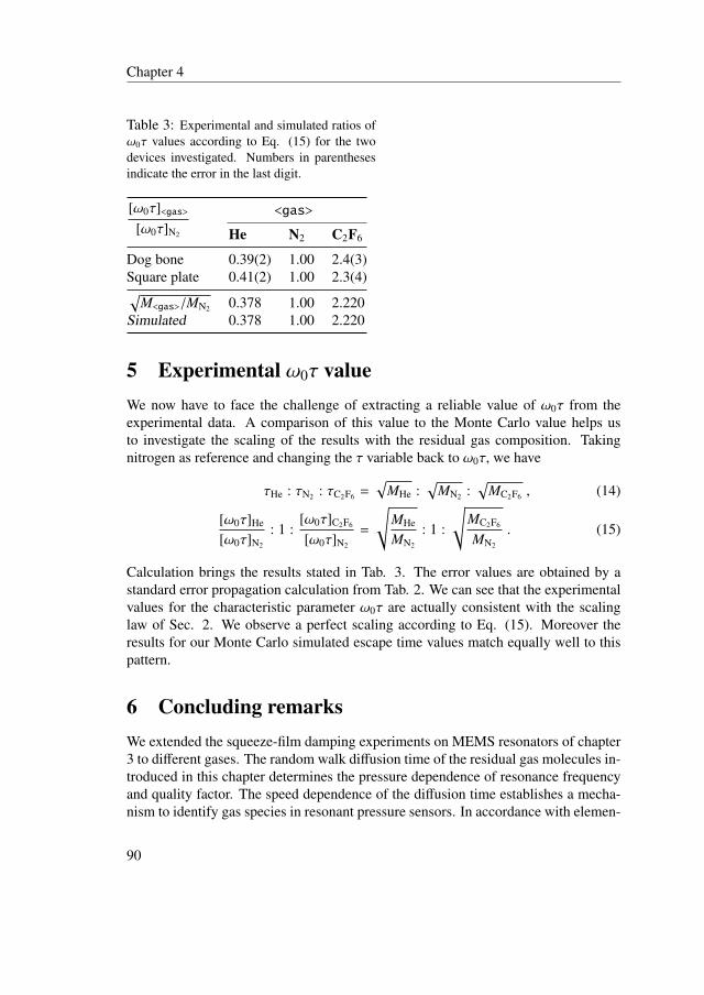
Model-based design of MEMS resonant pressure sensors Suijlen, M.A.G. DOI: 10.6100/IR716458 Published: 01/01/2011 Document Version Publisher’s PDF, also known as Version of Record (includes final page, issue and volume numbers) Please check the document version of this publication: • A submitted manuscript is the author's version of the article upon submission and before peer-review. There can be important differences between the submitted version and the official published version of record. People interested in the research are advised to contact the author for the final version of the publication, or visit the DOI to the publisher's website. • The final author version and the galley proof are versions of the publication after peer review. • The final published version features the final layout of the paper including the volume, issue and page numbers. Link to publication Citation for published version (APA): Suijlen, M. A. G. (2011). Model-based design of MEMS resonant pressure sensors Eindhoven: Technische Universiteit Eindhoven DOI: 10.6100/IR716458 General rights Copyright and moral rights for the publications made accessible in the public portal are retained by the authors and/or other copyright owners and it is a condition of accessing publications that users recognise and abide by the legal requirements associated with these rights. • Users may download and print one copy of any publication from the public portal for the purpose of private study or research. • You may not further distribute the material or use it for any profit-making activity or commercial gain • You may freely distribute the URL identifying the publication in the public portal ? Take down policy If you believe that this document breaches copyright please contact us providing details, and we will remove access to the work immediately and investigate your claim. Download date: 04. May. 2018
Transcript
Model-based design of MEMS resonant pressure sensors
Suijlen, M.A.G.
DOI:10.6100/IR716458
Published: 01/01/2011
Document VersionPublisher’s PDF, also known as Version of Record (includes final page, issue and volume numbers)
Please check the document version of this publication:
• A submitted manuscript is the author's version of the article upon submission and before peer-review. There can be important differencesbetween the submitted version and the official published version of record. People interested in the research are advised to contact theauthor for the final version of the publication, or visit the DOI to the publisher's website.• The final author version and the galley proof are versions of the publication after peer review.• The final published version features the final layout of the paper including the volume, issue and page numbers.
Link to publication
Citation for published version (APA):Suijlen, M. A. G. (2011). Model-based design of MEMS resonant pressure sensors Eindhoven: TechnischeUniversiteit Eindhoven DOI: 10.6100/IR716458
General rightsCopyright and moral rights for the publications made accessible in the public portal are retained by the authors and/or other copyright ownersand it is a condition of accessing publications that users recognise and abide by the legal requirements associated with these rights.
• Users may download and print one copy of any publication from the public portal for the purpose of private study or research. • You may not further distribute the material or use it for any profit-making activity or commercial gain • You may freely distribute the URL identifying the publication in the public portal ?
Take down policyIf you believe that this document breaches copyright please contact us providing details, and we will remove access to the work immediatelyand investigate your claim.
BirthFollowing its release in the early 1950s the transistor revolutionized the field of elec-tronics, and launched an extensive industry for miniaturized electronic circuits. Itreplaced the bulky vacuum tubes customary to amplifying and switching signals untilthen. Today the transistor is the fundamental building block of modern electronicdevices, and is ubiquitous to daily life technology. Obviously industry has undergonea tremendous development to create this massive spread. The major contribution ar-guably is the integration of circuit components in one and the same substrate material.Fifty years ago, Jack Kilby from Texas Instruments gave the outset to this integrationwith his primevally integrated circuit of a phase-shift oscillator [1]. He looked fora solution known as ”The Monolithic Idea” in which circuit elements as resistors,capacitors, distributed capacitors and transistors are all included in a single chip ofsemiconductor material. The integrated circuit’s mass production capability, relia-bility, and building-block approach to circuit design ensured the rapid adoption ofstandardized ICs in stead of designs using discrete transistors.
There are two main advantages of ICs over discrete circuits: cost and perfor-mance. Cost is low because the chips, with all their components, are printed as a unitby photolithography rather than being constructed one transistor at a time. More-over, much less material is used to construct a packaged IC die than a discrete circuit.Performance is high since the components switch quickly and consume little power(compared to their discrete counterparts) because the components are small and posi-tioned close together. As of 2010, chip areas range from a few to many tens of square
2
Chapter 1
millimeters, with up to three million transistors per mm2 (IBM z196 microprocessor)[2].
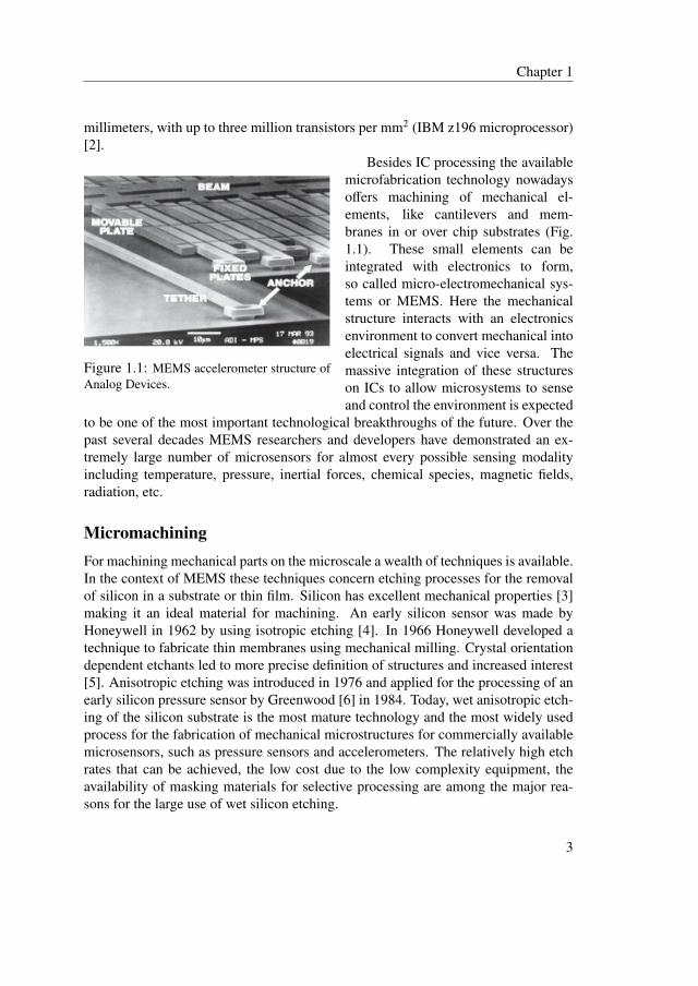
Besides IC processing the availablemicrofabrication technology nowadaysoffers machining of mechanical el-ements, like cantilevers and mem-branes in or over chip substrates (Fig.1.1). These small elements can beintegrated with electronics to form,so called micro-electromechanical sys-tems or MEMS. Here the mechanicalstructure interacts with an electronicsenvironment to convert mechanical intoelectrical signals and vice versa. Themassive integration of these structureson ICs to allow microsystems to senseand control the environment is expected
to be one of the most important technological breakthroughs of the future. Over thepast several decades MEMS researchers and developers have demonstrated an ex-tremely large number of microsensors for almost every possible sensing modalityincluding temperature, pressure, inertial forces, chemical species, magnetic fields,radiation, etc.
MicromachiningFor machining mechanical parts on the microscale a wealth of techniques is available.In the context of MEMS these techniques concern etching processes for the removalof silicon in a substrate or thin film. Silicon has excellent mechanical properties [3]making it an ideal material for machining. An early silicon sensor was made byHoneywell in 1962 by using isotropic etching [4]. In 1966 Honeywell developed atechnique to fabricate thin membranes using mechanical milling. Crystal orientationdependent etchants led to more precise definition of structures and increased interest[5]. Anisotropic etching was introduced in 1976 and applied for the processing of anearly silicon pressure sensor by Greenwood [6] in 1984. Today, wet anisotropic etch-ing of the silicon substrate is the most mature technology and the most widely usedprocess for the fabrication of mechanical microstructures for commercially availablemicrosensors, such as pressure sensors and accelerometers. The relatively high etchrates that can be achieved, the low cost due to the low complexity equipment, theavailability of masking materials for selective processing are among the major rea-sons for the large use of wet silicon etching.
3
Chapter 1
Figure 1.2: Typical bulk micromachined structures: a) membranes and beams, b) wafer-through holes, b) microwells.
If significant amounts of the substrate (bulk) material must be removed to re-lease a functional structure, the application of etching processes results in bulk mi-cromachining. Bulk micromachining can be accomplished using chemical or physi-cal means, with chemical means being far more widely used in the MEMS industry.Typical bulk micromachined structures, like wafer-through holes for interconnects inchip stacks and cavities/channels to form reservoirs for biochemical applications, areshown in Fig. 1.2.
Another very popular technology used forthe fabrication of MEMS devices is surfacemicromachining. Contrary to bulk microma-chining, the formation of microstructures is notrealized by etching for silicon removal in thewafer. It involves the deposition of additionallayers on the wafer surface and selectively re-moving one or more of these layers to leavefree-standing structures. There are a very largenumber of variations of how surface microma-chining is performed, depending on the mate-rials and etchant combinations that are used.However, the common theme involves a se-quence of steps (Fig. 1.3) starting with the de-position of some thin-film material to act asa sacrificial layer onto which the actual de-vice layers are built; followed by the deposi-tion and patterning of the thin-film device layerof material which is referred to as the structurallayer; then followed by the removal of the sac-rificial layer to release the mechanical struc-ture layer from the constraint of the underlying
4
Chapter 1
layer, thereby allowing the structural layer to move.Some of the reasons surface micromachining is so popular is that it provides for
precise dimensional control in the vertical direction. This is due to the fact that thestructural and sacrificial layer thicknesses are defined by deposited film thicknesseswhich can be accurately controlled. As a result of the commonly high fidelity ofthe photolithography and etch processes, surface micromachining also provides forprecise dimensional control in the horizontal plane. Other benefits of surface micro-machining are that a large variety of structure, sacrificial and etchant combinationscan be used; some are compatible with microelectronics devices to enable integratedMEMS devices. Surface micromachining frequently exploits the deposition char-acteristics of thin-films such as conformal coverage using LPCVD. Lastly, surfacemicromachining uses single-sided wafer processing and is relatively simple. Thisallows higher integration density and lower resultant cost per die compared to bulkmicromachining.
BenefitsBy far miniaturization is often the main driver of MEMS development. The commonperception is that miniaturization reduces cost, by decreasing material consumptionand allowing batch fabrication, but an important collateral benefit is also in the in-crease of applicability. Actually, reduced mass and size allow placing the MEMS inplaces where a traditional system would not be able to fit. Finally, these two effectsconcur to increase the total market of the miniaturized device compared to its costlierand bulkier predecessor. A typical example is found in the accelerometer developedas a replacement for traditional airbag triggering sensor and that is now used in manyappliances, as in digital cameras to help stabilize the image or even in the contactlessgame controller integrated in the latest cellphones. However often miniaturizationalone cannot justify the development of new MEMS. After all if the bulky compo-nent is small enough, reliable enough, and particularly cheap then there is probablyno reason to miniaturize it. Micro-fabrication process cost cannot usually competewith metal sheet punching or other conventional mass production methods.
But MEMS technology allows something different, at the same time you make thecomponent smaller you can make it better. The airbag crash sensor gives us a goodexample of the added value that can be brought by developing a MEMS device. Somenon-MEMS crash sensors are based on a metal ball retained by a rolling spring or amagnetic field. The ball moves in response to a rapid car deceleration and shortstwo contacts inside the sensor. A simple and cheap method, but the ball can beblocked or contact may have been contaminated. Moreover, when your start yourengine, there is no easy way to tell if the sensor will work or not. MEMS devicescan have a built-in self-test feature, where a micro-actuator will simulate the effect of
5
Chapter 1
deceleration and allow checking the integrity of the system every time you startup theengine. Another advantage that MEMS can bring relates with the system integration.Instead of having a series of external components (sensor, inductor...) connected bywire or soldered to a printed circuit board, the MEMS on silicon can be integrateddirectly with the electronics. Whether it is on the same chip or in the same package itresults in increased reliability and decreased assembly cost, opening new applicationopportunities. As we see, MEMS technology not only makes the things smaller butoften makes them better.
DriversFrom the heyday of MEMS research at the end of the 1960s, one main driver forMEMS development has been the automotive industry. It is really amazing to seehow many MEMS sensor a modern car can use! From the first oil pressure sensors,car manufacturers quickly added manifold and tire pressure sensors, then crash sen-sors, one, then two and now up to five accelerometers. Recently the gyroscopes madetheir apparition for anti-skidding systems and vehicle navigation – the list seems with-out end. Miniaturized pressure sensors were also quick to find their ways in medicalequipment for blood pressure testing. Since then biomedical applications have at-tracted a lot of attention from MEMS developers. The DNA chip and micro totalanalysis system (µTAS) are the latest successes in the list. Because you usually sellmedical equipment to doctors and not to patients, the biomedical market has manyfeatures making it perfect for MEMS: a niche market with large added value.
Actually cheap and small MEMS sensors have many applications. Digital cam-eras have been starting using accelerometers to stabilize image, or to automaticallyfind image orientation. Accelerometers are also being used in new contactless gamecontrollers. These two latter products are just a small part of the MEMS-based sys-tems that the computer industry is using to interface digital input-output with ourhuman senses. The inkjet printer, DLP based projector, head-up display with scannermirror are all MEMS based computer output interfaces. Additionally, computer massstorage uses an abundant amount of MEMS, for example, hard-disk drives nowadaysconsist of a micromachined GMR head and dual stage MEMS micro-actuator. Ofcourse in that last field more innovations are in the labs, and most of them use MEMSas the central reading/ writing element.
The telecommunication industry has fueled the biggest MEMS R&D effort so far.Especially the wireless telecommunication business is using more and more MEMScomponents to deal with the demand for ever increasing functionality of portable de-vices on the one hand and their limited size and battery capacity on the other hand.MEMS are slowly sipping into cellphones replacing discrete elements one by one, RFswitch, microphone, filters – until the dream of a 1 mm3 cellphone becomes true (with
6
Chapter 1
vocal recognition for numbering of course!). The latest craze is in using accelerom-eters (again) inside cellphones to convert them into game controllers, the ubiquitouscellphone becoming even more versatile.
Finally, it is in spacecraft that MEMS are finding an ultimate challenge and al-ready some MEMS sensors have been used in satellites. The development of micro(less than 100 kg) and nano (about 10 kg) satellites is bringing the mass and vol-ume advantage of MEMS to good use and some projects are considering swarms ofnanosatellites populated with micromachined systems.
In spite of the interest for numerous new (exotic) sensing applications, MEMStechnology arguably has even more significance to system integration and miniatur-ization of existing microelectronic building blocks. An emerging class of MEMStakes on this challenge for the ubiquitous reference oscillator [7, 8, 9]. This ele-ment is used for a wide range of applications varying from keeping track of real-time,setting clock frequency for digital data transmission, frequency up- and down con-version in RF transceivers, and clocking of logic circuits. It involves a multi-billiondollar market in today’s electronic industry.
1.2 MEMS oscillatorsOscillator technologies for mainstream electronic applications are either based onmechanical or electrical resonance [10]. Mechanical resonators are typically madefrom a piezo-electric material such as quartz onto which a pair of metal electrodes isplaced to allow for energy transfer between the mechanical domain – the resonator –and the electrical domain: the feedback amplifier for sustaining the oscillation. Theoscillation frequency is set by the physical dimensions of the resonator body and theposition of electrodes on it.
One of the properties setting mechanical resonators apart from electrical res-onators is a high quality factor (Q) which is imperative to make oscillators with lownoise level work. A mechanical resonator material known of old for its pronouncedlyhigh quality factor is the quartz crystal. Thanks to this property and a very high sta-bility – for certain crystal cuts – of the resonance frequency to temperature change,quartz based oscillators have become known for coupling superior accuracy to min-imal temperature drift and noise [11]. Quartz is the technology of choice where os-cillator noise and stability are most demanding such as for wireless communication(e.g. GSM, Bluetooth), but also high-speed digital serial-interfaces (e.g. USB2.0,real-time clocks).
The Q-factor, stability, and temperature drift of ceramic resonators made frome.g. barium titanate or lead-zirconium titanate tends to be smaller than for quartz,but ceramic resonators are cheaper to produce [12]. Therefore, ceramic resonators
7
Chapter 1
are used for applications where frequency stability and noise is less of a concern, butwhere the oscillator performance nevertheless cannot be met with electrical oscilla-tors. Ceramic resonators are mainly used in consumer applications such as remotecontrols, digital audio/video, and household appliances.
Although the electrical performance of mechanical oscillators cannot be met byelectrical oscillators, mechanical oscillators have some important drawbacks that pre-vent their use in every application. Mechanical resonators are relatively bulky andcannot be embedded in the IC chip. Combining them with the chip package that pro-vides more space, on the other hand, would increase the manufacturing complexityand cost too much. Therefore, mechanical resonators have to interface with othercircuit components on board level and therefore form a bottleneck for the ultimateminiaturization of the electronic system.
On the other hand, oscillators based solely on electronic components such asresistor-capacitor (RC), inductor-capacitor (LC), or ring oscillators can be integratedon CMOS chips. However, their use is limited to applications, e.g. processor clocks,were accuracy and noise specification is relaxed. Their stability and near-carrier noisecan be improved by locking them to mechanical oscillators using a phase-locked loop(PLL). However, this requires again a bulky off-chip component adding to the totalsize and cost of the system.
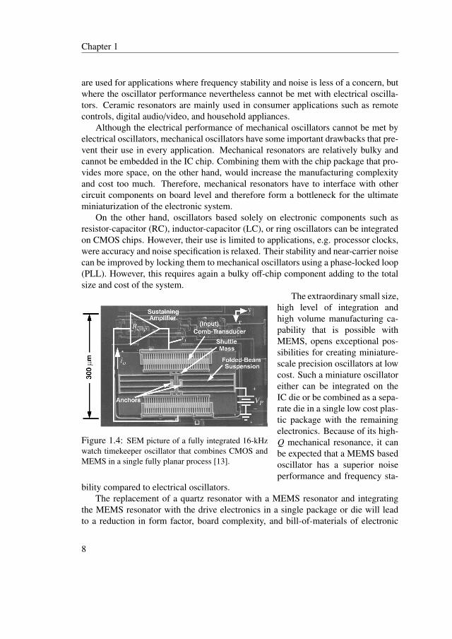
Figure 1.4: SEM picture of a fully integrated 16-kHzwatch timekeeper oscillator that combines CMOS andMEMS in a single fully planar process [13].
The extraordinary small size,high level of integration andhigh volume manufacturing ca-pability that is possible withMEMS, opens exceptional pos-sibilities for creating miniature-scale precision oscillators at lowcost. Such a miniature oscillatoreither can be integrated on theIC die or be combined as a sepa-rate die in a single low cost plas-tic package with the remainingelectronics. Because of its high-Q mechanical resonance, it canbe expected that a MEMS basedoscillator has a superior noiseperformance and frequency sta-
bility compared to electrical oscillators.The replacement of a quartz resonator with a MEMS resonator and integrating
the MEMS resonator with the drive electronics in a single package or die will leadto a reduction in form factor, board complexity, and bill-of-materials of electronic
8
Chapter 1
circuits. Here, the device of Nguyen and Rowe [13] (Fig. 1.4) with its resonatorstructure and electronics in a single fully planar process shows how far integrationcan go. Simultaneously, the MEMS solution will have an improved electrical perfor-mance compared to LC, RC, or other types of oscillators based on electrical ratherthan mechanical resonance. These unique attributes reduce the size and cost of ex-isting electronic systems, and might open up new application domains, e.g. wirelesssensor nodes [14] or other products requiring extreme form factor such as SIM andsmartcards.
1.2.1 MEMS resonator packaging
As MEMS oscillators need vacuum conditions in the sub-mbar range for proper andreliable operation of the resonator, the packaging process of these devices must pro-vide direct caps to the resonators that seal them hermetically. The resonators arebrought in evacuated cavities by sealing them in a vacuum environment. The endpressure inside the package then is expected to equal the pressure level of this sealingenvironment. Two process families can be distinguished for the batch fabrication ofthese microcavities [10].
The most mature method is based on the bonding of two wafers [15]. In thiscase, the wafer containing the MEMS resonator has a seal ring which fits to a facingring on the capping wafer. A cavity is created around the resonator after bondingthe two wafers together. For further processing the different resonators are singulatedfrom the wafer. Although wafer-to-wafer bonding is a relatively mature techniquethat is also used for the packaging of e.g. accelerometers and gyroscopes, it has thedisadvantage that a large amount of valuable wafer area is required for the sealingring. This not only results into a large product, but also increases the manufacturingcost since fewer resonators per wafer can be processed. Furthermore, the height ofthe packaged resonator is set by the combined thickness of two wafers. Therefore,wafer bonding sealing can lead to a package size that is many times the size of theresonator residing inside the cavity.
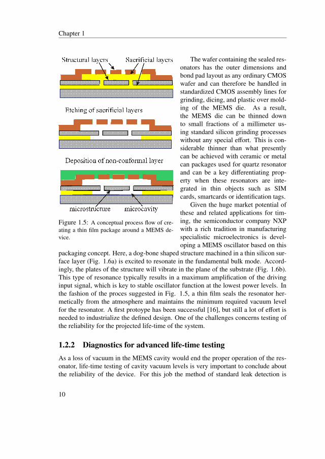
A more advanced on-wafer sealing method leading to a much smaller packageis based on surface micromachining. A schematic process flow for the fabricationof the resonator cap is shown in Fig. 1.5. Here sacrificial layer etching and coatingtechniques are used to create a microcavity around the resonator. The advantage ofsurface micromachining is that the size of the cavity is only slightly larger than thesize of the resonator itself. As a result, die size remains small which will lead to a costbenefit, since a large amount of devices can be processed onto a single wafer. Theheight of the sealed resonator is now set by the thickness of a single wafer instead ofthe combined thickness of two wafers in case of wafer-to-wafer bonding.
9
Chapter 1
Figure 1.5: A conceptual process flow of cre-ating a thin film package around a MEMS de-vice.
The wafer containing the sealed res-onators has the outer dimensions andbond pad layout as any ordinary CMOSwafer and can therefore be handled instandardized CMOS assembly lines forgrinding, dicing, and plastic over mold-ing of the MEMS die. As a result,the MEMS die can be thinned downto small fractions of a millimeter us-ing standard silicon grinding processeswithout any special effort. This is con-siderable thinner than what presentlycan be achieved with ceramic or metalcan packages used for quartz resonatorand can be a key differentiating prop-erty when these resonators are inte-grated in thin objects such as SIMcards, smartcards or identification tags.
Given the huge market potential ofthese and related applications for tim-ing, the semiconductor company NXPwith a rich tradition in manufacturingspecialistic microelectronics is devel-oping a MEMS oscillator based on this
packaging concept. Here, a dog-bone shaped structure machined in a thin silicon sur-face layer (Fig. 1.6a) is excited to resonate in the fundamental bulk mode. Accord-ingly, the plates of the structure will vibrate in the plane of the substrate (Fig. 1.6b).This type of resonance typically results in a maximum amplification of the drivinginput signal, which is key to stable oscillator function at the lowest power levels. Inthe fashion of the proces suggested in Fig. 1.5, a thin film seals the resonator her-metically from the atmosphere and maintains the minimum required vacuum levelfor the resonator. A first protoype has been successful [16], but still a lot of effort isneeded to industrialize the defined design. One of the challenges concerns testing ofthe reliability for the projected life-time of the system.
1.2.2 Diagnostics for advanced life-time testingAs a loss of vacuum in the MEMS cavity would end the proper operation of the res-onator, life-time testing of cavity vacuum levels is very important to conclude aboutthe reliability of the device. For this job the method of standard leak detection is
10
Chapter 1
(a) SEM picture of processed structure. (b) Result of eigenmode simulation showing thedeformation during in-plane vibration.
Figure 1.6: NXP’s dog-bone shaped resonator for high frequency timing purposes processedin silicon-on-insulator (SOI). This structure is intended to perform high frequency in-planeresonant oscillation.
rather insensitive and absolute pressure sensors may be integrated in the wafer-levelpackaging for in-situ testing of the cavity vacuum. Waelti et al. [17] and Mailly etal. [18] for example present some solutions with dedicated sensors in the packagebased on measurement of the thermal conductivity of the residual gas. At the millibarrange vacuum pressures in typical cavities, this conductivity is directly proportionalto the gas density which enables measurement of absolute pressure. These wafer-levelPirani-type pressure sensors exist in many geometrical and read-out implementationsthat can be tailored to a wide range of sensitivities either with or without linear re-sponse behavior. See for example Li et al. [19] for a state-of-the-art sensor design.
All these solutions however disregard the resonator structure itself as pressuresensor. After all, the trouble about vacuum packaging follows from the resonator’ssusceptibility to gas pressure in the first place. Given this principle sensitivity, causedby the momentum transfer between resonator structure and gas molecules, the re-alization of a pressure sensor with specified sensitivity and range is all a matter ofdesign. In the ideal case, a read-out of the common characteristics in resonant op-eration (quality factor and resonance frequency) of the resonator sample could besufficient to measure the absolute cavity pressure without any additional structuresand signal conversion!
11
Chapter 1
1.2.3 PhD on design
Motivated by the need of diagnostics for advanced life-time testing of thin-film pack-aged MEMS resonators, a project for the conceptual design (in Dutch ’proefontwerp’)of such resonant pressure sensors was initiated at the NXP production and innovationcenter in Nijmegen. After a project with preliminary design results performed at thiscenter as part of preceding education [20], work was continued at the laboratoriesof NXP Research in Eindhoven. Activities were an integral part of NXP’s businesscase to develop MEMS oscillators on 1.5 µm SOI substrates [21]. The output ofthe PhD on design project includes several device prototypes, two invention disclo-sures [22, 23], a contributed talk at the Eurosensors XXII conference [24] and newdiagnostic measurement methods. The focus of this thesis is on the presentation andevaluation of the actual designed/invented processes or devices.
By chance, NXP agrees with a wide dissemination of the results in the thesis.Also, the knowledge developed in the present project connects to a timely field ofstudy in the open literature. For this reason, the chapters in the body of this thesis arewritten in the format of a journal paper, for future publication in scientific journals.This will bring our findings out into the open beyond the current network at TU/eand NXP. The text of chapter 2 has been published in ”Sensors and Actuators A”,Ref. [25]; chapter 3 was submitted lately to the same journal but was not acceptedfor publication due to a lack of comparison of our model results with other modelsin literature. A fully revised version, splitting up the model calculations and theexperimental results in two separate papers, is foreseen in the future.
Chapter 4, which has been added at a very late stage of writing the thesis, stillneeds major work to qualify as a manuscript for a journal (e.g., adding references toliterature). For the purpose of providing sufficient insight in the process of design,its current shape is acceptable. Because it deals with the role of gas species in ourmodel thus and directly connects to chapter 3, this sets a certain order in time on itspublication.
1.2.4 This thesis
Modeling and simulation of the forces that the gas exerts on the resonator structureplays a major role for this design task. If the approach should be used in industry,values of pressure sensitivities for every version designed need to be available with-out time-consuming measurements. Also specifying the spread in pressure sensitivityof resonators due to process spread in the design parameters calls for proper model-ing. Absolute accuracy in this respect is not as important as efficiently gaining clearinsights in the physical processes involved.
The narrow gaps of resonators cause a strong coupling of microstructure move-
12
Chapter 1
ment with the flow of residual gas and the emerging squeeze-film forces turn out to bethe determining gas-structure interaction in typical resonators. Quantitative predic-tion of the gas flow and resulting forces involves in existing squeeze-film models gen-erally a highly specialistic programming effort and this seriously complicates properdesign activities. Therefore we developed a new, semi-analytical model that can liveup to the standards of efficient designing. It is revealed and validated in chapters 2, 3and 4 of this thesis.
Building on the knowledge and ideas from all our experiments, chapter 5 presentsan analysis and evaluation of our design solution to sensitive cavity vacuum testingin MEMS resonators. It illustrates and supports the method and sensor design weclaimed in the patent application of Ref. [26]. The result shows pressure sensingwith the resonator is useful to life-time testing during fabrication and model-baseddesign of MEMS resonant pressure sensors is a reality. Next, chapter 6 discusses witha comparison of published data on the squeeze-film damping for different resonatordesigns the value of our model to generic resonator design.
Finally, chapter 7 concludes and summarizes this thesis.
13
Bibliography
[1] J.S. Kilby, IEEE Trans. Electron Devices 23 (7) 1976.
[2] Shvets, Anthony, ”IBM is ready to ship the fastest microprocessor,”CPU-World.com, (September 5, 2010).
[13] C. T.-C. Nguyen and R. T. Howe, IEEE J. Solid-State Circ. 34 (4) (1999) 440-455.
[14] C.C. Enz, J. Baborowski, J. Chabloz, M. Kucera, C. Muller, D. Ruffieux, N.Scolari, Proc. European Conference on Circuit Theory and Design (ECCTD)2007, 320-331.
14
Chapter 1
[15] R. Pelzer, H. Kirchberger, P. Kettner, Proc. Int’l Conf. Electronic PackagingTechnology (ICEPT) 2005, 1-6.
[17] M. Waelti, N. Schneeberger, O. Paul, H. Baltes, Int. J. Microcircuits and Elec-tronic Packaging 22 (1) (1999) 49-56.
[18] F. Mailly, N. Dumas, N. Pous, L. Latorre, O. Garel, E. Martincic, F. Verjus, C.Pellet, E. Dufour-Gergam, P. Nouet, Sens. and Actuators A 156 (2009) 201-207.
[19] Q. Li, J.F.L. Goosen, J.T.M. van Beek, F. van Keulen, Sens. Actuators A 162(2010) 267-271.
[20] M.A.G. Suijlen, ”Ontwerp MEMS druksensor: rapport ontwerpproject NXPNijmegen”, Final report Stan Ackermans Institute TU/e, 2007.
[21] J.J.M. Bontemps, ”Design of a MEMS-based 52 MHz oscillator,” PhD thesisTU/e, 2009.
[23] M.A.G. Suijlen, J.J. Koning, H.C.W. Beijerinck, ”Molecular mass detection ofa gas using a spring damped resonant pressure microsensor,” ID81410650 NXP,2010.
[24] M.A.G. Suijlen, J.J. Koning, M.A.J. van Gils, H.C.W. Beijerinck, Proc. Eu-rosensors XXII, Dresden, 2008.
[25] M.A.G. Suijlen, J.J. Koning, M.A.J. van Gils, H.C.W. Beijerinck, Sens. Actua-tors A 156 (2009) 171-179.
[26] Matthijs Suijlen, Jan-Jacob Koning, Herman Coenraad Willem Beijerinck,”MEMS pressure sensor,” patent application US2011/0107838 A1.
15
Chapter 2
Squeeze film damping in thefree molecular flow regime withfull thermal accommodation
We introduce an analytical model for the gas damping of a MEMS resonatorin the regime of free molecular flow. Driving force in this model is the change indensity in the gap volume due to the amplitude of the oscillating microstructure,which is counteracted by the random walk diffusion in the gap that tries to re-store the density to its equilibrium value. This results in a complex-valued forcethat contributes to both the damping as well as the spring constant, depending onthe value of ωτ with ω the resonance frequency and τ the random walk diffusiontime. The diffusion time is calculated analytically using the model for randomwalk Brownian motion and numerically by a Monte Carlo simulation of the bal-listic trajectories of the molecules following Maxwell-Boltzmann statistics andfull thermal accommodation in gas-surface collisions. The model is verified bycomparison to accurate data on the pressure dependency of the damping of threeMEMS resonators, showing agreement within 10 %.
1 IntroductionIn the study of the dynamic behavior of MEMS devices, damping forces resultingfrom surrounding air generally play a significant role. As the most commonly usedtechnologies are capacitive sensing and electrostatic driving, for which narrow airgaps often result, the so-called squeeze film effect dominates the interaction of the sur-rounding air with the moving part of a MEMS device. This effect refers to the pump-ing action of a fluid between closing up parallel surfaces with a gap much smallerthan their dimensions. It exceeds the drag force on the MEMS part that would beexperienced in isolated motion considerably. Current descriptions of squeeze film airdamping are derived considering a continuum fluid picture of the flow in the squeezefilm [1, 2, 3]. In many MEMS, however, squeeze film flow cannot be regarded ascontinuum-like. Gases trapped in the MEMS cavity often are so rarefied that themolecular mean free path exceeds the gap dimensions by at least an order of mag-nitude and flow becomes ’free molecular’. In this regime, intermolecular collisionsin the gap volume are increasingly rare. Thus the way to meaningfully describe theinteraction of MEMS parts with the gas is to consider the sum of all individual wallcollisions. Momentum is transferred between the gas molecules and the surface byballistic trajectories and wall collisions. For a stationary device, kinetic gas theoryshows that the net effect of the momentum transfer in all these collisions equals thepressure forces exerted on the surface.
For a non-stationary device such as a MEMS oscillator, simple kinetic gas theoryagain can be applied, showing an extra contribution to the force exerted on the surfacewhich is proportional to the plate velocity |~V | and counteracts the movement. This ismostly referred to as kinetic damping. It can be easily understood if we consider
18
Chapter 2
the simplified case of an elastic collision. Ballistic molecules hit the moving surfacewith a relative velocity that is larger (or smaller) by an amount |~V |, resulting in anextra contribution to the momentum transfer as compared to the stationary situation.Kinetic damping always occurs and is not unique for a MEMS device with a smallgap volume.
The effect of kinetic damping is rather small and models based on this effect[4, 5, 6, 7, 8] underestimate experimental values of the gas damping observed inMEMS devices [9]. Several approaches have been used to resolve this discrepancy.Of these approaches, the model of Bao et al. [10] is most relevant for our purpose ofestablishing an analytical model, as it explicitly appeals to the molecular motion ofthe flow in the gap. It shows reasonable agreement with experimental observationsof air damping on resonators with a beam-like geometry [11] with a large length-to-width ratio. However, to explain all the kinetic energy losses of the plate, Baointroduces an extra transfer of momentum beyond the normal molecule-surface inter-action. For this mechanism, he chooses the phenomenon of large number of consecu-tive elastic collisions, adding 2m Vz to the molecule’s momentum after each collisionwith the plate. Here, the z-direction coincides with the velocity vector ~V of the os-cillating plate. Even if, once in a while, a single elastic collision would occur, it isextremely unlikely to suppose that a sequence of hundreds of these collisions wouldoccur.
Considering the large body of data on the nature of collisions of molecules withsurfaces (see for example references 25-27 of Martin et al. [12]), we have to con-clude that practically all collisions happen to be inelastic. The relevant number isthe accommodation coefficient that is always close to unity for all (industrial) sur-faces in a moderate vacuum. This implies that, every time a molecule hits a wall,the molecule’s state is lost and reset to a new random state distributed accordingto Maxwell-Boltzmann statistics. For example, even in highly sophisticated beam-surface collision experiments under conditions of ultra-high vacuum, it requires amajor effort (baking at high temperature, sputtering, dips before entering the vac-uum) to clean the (single crystal) surface before the phenomenon of elastic collisionsis observed. Full thermal accommodation is the rule, elastic collisions are the excep-tion.
2 Squeeze film dampingIn this paper we consider the increase in density of the gas in the gap volume as thedriving force for the squeeze film damping in the regime of free molecular flow. Whenthe gap height decreases due to the plate movement, we see that the volume belowthe plate decreases accordingly. This results in a corresponding increase in number
19
Chapter 2
Figure 1: In-plane diffusion by single molecule random walk in a MEMS cavity
density. In an alternative picture, we can also state that the frequency of collisionswith the plate increases correspondingly, due to the shorter gap crossing time of eachmolecule. These pictures are equivalent, as we expect from the molecular picture ofBoyle’s law. A different value of the number density results in a different pressureexerted on the plate. The net effect of this change in pressure (or number density)depends on its phase as compared to the phase of the oscillating plate.
The in-phase component just acts as an extra contribution to the spring constantof the suspension of the plate. The out-of-phase component of the change in pressure(or number density) acts as a damping force for the plate. This is independent of themodel for the molecule-surface interaction – elastic or full accommodation. On thesingle molecule level, each collision has the same role of reversing the momentumof the molecule perpendicular to the surface, as is the case when it hits the wall of avacuum chamber. No particular molecular kinetics need to be considered. Until now,this effect has not been considered for modeling the squeeze film interaction in thefree molecular flow regime.
Because the gas will not move instantaneously, the phase shift is induced by thetime constant τ of the molecular diffusion to equalize the pressures in- and outside thegap. For high oscillation frequencies ω � 1/τ, the diffusion cannot respond to theincreasing density and we expect that the squeeze film will only influence the springconstant. For low oscillation frequencies ω � 1/τ, the density in the gap volume canrespond and the 90◦ phase shift in the density variations with respect to the amplitude
20
Chapter 2
Figure 2: Frequency dependence of the elastic force constant and the damping constant dueto the squeeze film interaction.
z will result in extra damping of the microstructure.
In section 3 we derive an analytical model for squeeze film damping based on thisbehavior. We also compare the results for the damping to the predictions of kineticdamping, showing that the first effect is much larger than the latter. Experimentson three MEMS oscillators are presented in section 4 showing a behavior that is inagreement with the model predictions. The pressure dependent damping coefficientis used to derive reliable values of the diffusion time τ.
In sections 5 and 6 we describe the diffusion of the molecules in the gap volume,applying full thermal accommodation in molecule-wall interactions. The moleculeswill perform a random walk in the cavity, bouncing up and down between microstruc-ture and substrate and erratically zigzagging along its trajectory as projected in theplane of the device. This is illustrated in Fig. 1. Our analysis is substantiated both inthe theoretical framework used to describe random walk in Brownian motion and ina fully numerical Monte Carlo simulation of the individual gas molecules.
With the validity of our model established in section 7 we put the good agree-ment of the damping on the microbeam resonator of Zook [11] with Bao’s model inperspective.
21
Chapter 2
3 Model
3.1 Squeeze force dampingThe increase in density of the gas in the gap volume is the driving force for thesqueeze film damping in the regime of free molecular flow. The density variation∆n(t) in the gap volume is governed by the differential equation
ddt
(∆nn
)= −1
τ
∆nn− d
dt
( zd
), (1)
with τ the random walk diffusion time, n the equilibrium value of the density, andz the coordinate pointing up from the plate (cf. Fig. 1) with z = 0 correspondingto its equilibrium position. The equation describes the rate of change in density, ascounteracted by the random walk diffusion (first term) and driven by the displacementz of the plate (second term). Assuming a forced plate oscillation with displacementz(t) = z0 eiωt and a trial solution ∆n(t)/n = (∆n0/n) eiωt with complex amplitude, wefind
∆n(t)n
= − z(t)d
iωτiωτ + 1
. (2)
In case of isothermal density variations ∆n(t), the force exerted on the plate is givenby
Fsqueeze = ∆n(t) kB T A = ∆p(t) A, (3)
with ∆p(t) the increase in pressure in the gap volume and A the frontal area of themoving plate. Combining Eqs. (2) and (3) the squeeze force Fsqueeze of the gas in thecavity on the moving plate thus satisfies
Fsqueeze = − p Ad
iωτ1 + iωτ
z, (4)
consisting of a real and imaginary contribution. The squeeze force Fsqueeze has to beinserted into the differential equation of the damped harmonic oscillator describingthe plate motion. The real part of the force Fsqueeze is in counter-phase with theamplitude z and results in an extra contribution −ksqueezez to the elastic force on theoscillating mass m of the MEMS; the imaginary part of Fsqueeze is out of phase withthe amplitude z, i.e., in counter-phase with the velocity z, and results in an additionaldamping −bsqueezez. The differential equation can now be written as
mz + bz + kz = F0 eiωt (5)
22
Chapter 2
with
b = bmat + bsqueeze (6)k = kmat + ksqueeze. (7)
Here, bmat and kmat represent the inherent damping and stiffness of the mechanicalstructure. The contributions due to the complex valued squeeze force are given by
bsqueeze =p A τ
d1
1 + (ωτ)2 (8)
ksqueeze =p Ad
(ωτ)2
1 + (ωτ)2 . (9)
In a plot of these parameters versus frequency ω (Fig. 2), one can clearly see thecharacter of the squeeze film interaction: for low frequency oscillations, ω � 1/τ, itmanifests itself as pure damping force and for rapid oscillations, ω � 1/τ, it becomesan elastic force without damping. These results show how we can optimize the designof MEMS resonators. E.g., for an application as a pressure sensor, we have to chooseωτ = 1 for maximum sensitivity. To avoid a shift in the operating frequency, we canchoose ωτ = 0.3, with a slight trade-off in maximum sensitivity. Conversely, to usea frequency shift as pressure read-out instead of the change in quality factor, we canchoose ωτ > 3 as range of operation.
Alternatively, similar results for the damping coefficient bsqueeze and spring con-stant ksqueeze are obtained when solving the density profile in the gap n(x, t) in thetime domain from the common diffusion equation. The diffusion coefficient D thenfunctions as the inverse random-walk diffusion-time 1/τ from Eq. (1). Instead of themean free path λ of the molecules to estimate the diffusion coefficient one has to usethe gap width d here, being by far the smallest of the two in the regime investigated.
3.2 Kinetic dampingThe squeeze force damping has to be compared to the kinetic damping bkin due tomomentum transfer of the molecules impinging on the surface of the plate. Thisdamping effect is always effective at conditions of free molecular flow, irrespectiveof the specific geometry of the plate and its surroundings. Both surfaces of the platecontribute. Christian [13] has shown that
bkin = (16/π)(pA/〈v〉) , (10)
with 〈v〉 the average velocity of the gas molecules and p the equilibrium value of thepressure. Neglecting the pressure variations in the gap is fully justified for inspect-ing the influence of kinetic damping, because this is a only a second order effect.
23
Chapter 2
Comparing this result to squeeze film damping at ωτ � 1, where the ω-dependencydisappears, we find
bsqueeze/bkin = (π/16)〈v〉/vgeom , (11)
with vgeom = d/τ an effective velocity that depends on the geometry of the resonatorplate. For MEMS resonators, typical values of the gap width d are in the 1 to 3 µmrange. The diffusion time is on the order of 0.1 to 0.5 µs, as we will show in the fol-lowing sections 4, 5 and 6. Thus 2 m/s < vgeom < 30 m/s which should be comparedto typical molecular velocities, with 〈v〉 = 471 m/s for N2 at room temperature. Weconclude that for typical MEMS resonators in the range ωτ < 1 squeeze dampingdominates by far over kinetic damping. For ωτ � 1 the squeeze damping decreasesproportional to (ωτ)−2 and the kinetic damping is finally the only remaining effect.
4 Experiments
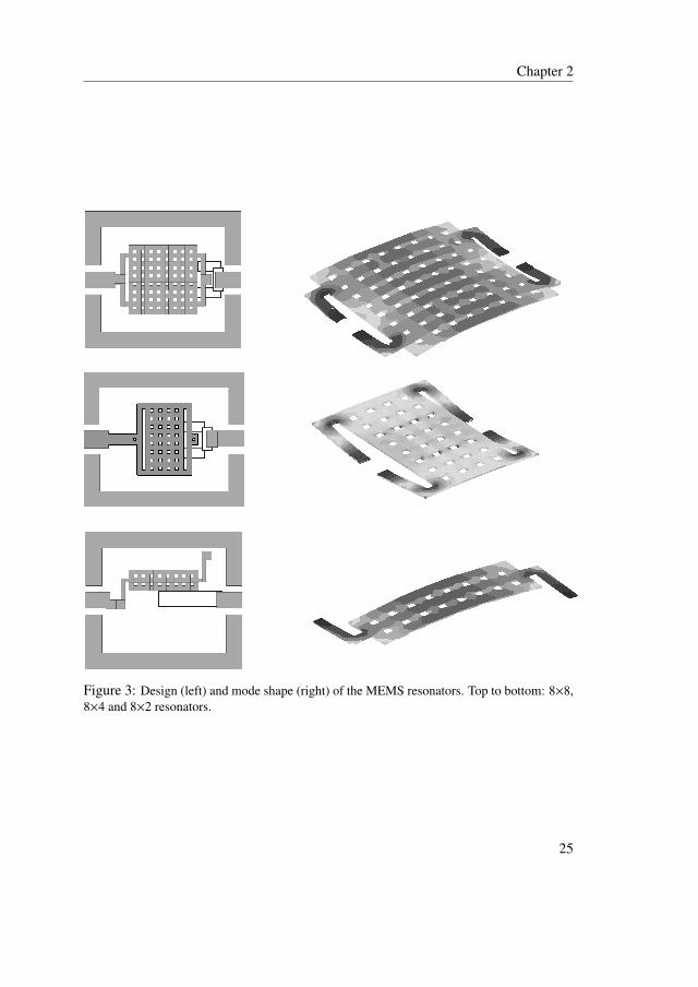
To test the model, we have investigated the pressure dependency of the damping co-efficient of three different resonators. These devices were designed as switches witha low stiffness suspension and thus a low resonance frequency. By chance, they arewell suited to test our model of squeeze film damping. The devices consist of a rect-angular aluminum plate supported by cantilever beams above the substrate. The plateis provided with 18 × 18 µm2 sized etch holes in a 50 µm pitch, square grid. Theseetch holes have been used for the sacrificial etch to open the gap. The gap distancebetween plate and substrate is d = 3 µm for all devices. The substrate is coatedwith a thin metallic layer. The devices are labeled ’8×8’, ’8×4’ and ’8×2’, referringto their etch hole grid. The characteristic dimensions are given in Tab. 1. The fre-quency ω0,mat and spring constant kmat are derived from a finite element simulationof the device using ”COMSOL Multiphysics”. In this calculation the spring constantkmat is defined by equating the total strain energy Ustrain(t) of the microstructure to12 kmat zmax(t)2, with zmax(t) the maximum value of the microstructure’s deflection attime t. In Fig. 3 we show the actual layout of the devices and the shape of the lowestmode of vibration, calculated using COMSOL.
The devices are not packaged in a vacuum tight enclosure: they interact with thesurrounding residual gas. At the edges, the open area between the support beams andthe plate is sufficiently large for gas molecules to enter or leave the gap between plateand substrate. To measure the pressure dependency of the devices, we mount them ina vacuum chamber with a base pressure less than 1 × 10⁻⁵ mbar. With a leak valvewe introduce N2 gas to achieve the desired pressure in the 1 to 10 mbar range. Thepressure is measured with an MKS Baratron 627B capacitance manometer with anaccuracy of 0.12%.
24
Chapter 2
Figure 3: Design (left) and mode shape (right) of the MEMS resonators. Top to bottom: 8×8,8×4 and 8×2 resonators.
25
Chapter 2
Table 1: Characteristic dimensions of the three MEMS devices, together with the reso-nance frequency ω0,mat, spring constant kmat and mode shape factor γ as calculated froma finite element simulation using COMSOL. The calculation of the spring constant usesUstrain(t) = 1
2 kmat zmax(t)2 with zmax(t) the maximum value of the microstructure’s deflection.
Figure 4: Typical experimental results of the resonances for the investigated MEMS res-onators
26
Chapter 2
The electrical readout of the amplitude of the oscillating plate is straightforward.The aluminium plate and a thin metal layer deposited on the substrate form a vari-able capacitor. Plate motion was detected via capacitance changes measured usingan HP4294 impedance analyzer. At resonance, the plate amplitude rises and moremechanical energy is dissipated in the ambient gas. Since this dissipated energy mustbe supplied by the analyzer, a peak is seen in the magnitude of the admittance. Wemeasure both the frequency response of the device to determine the quality factor aswell as the ohmic dissipation on resonance. Both methods are in good agreement andresult in a measure of the damping coefficient b. Only the ’8×8’ device results in30% larger values of b with the latter method. However, the large dependency of thedamping b ∝ d−4 on the gap width d suggests that the sacrificial etch for the ’8×8’device perhaps is incomplete, with a 7.5% smaller value of d as result. As yet wehave no definitive explanation for the observed discrepancy.
Typical experimental results are shown in Fig. 4. For five different values of thepressure in the vacuum chamber, ranging from 1.0 to 5.1 mbar, the resonance signalof the 8×8 device is shown as a function of the generator frequency. We clearly seethe decrease of the quality factor with increasing pressure. We also observe that theshift of the resonance frequency is very small and nearly drowns in the errors of themeasurement. We estimate an upper limit on the order of 20 Hz/mbar. We have tocompare this result with the prediction of Eq. 9, with a maximum frequency shift forωτ � 1 given by
1ω
dωdp
=12k
dksqueeze
dp=
12k
Ad. (12)
For the 8×8 device we find a predicted maximum frequency shift of 10 kHz/mbardue to squeeze forces, more than two orders of magnitude larger than observed ex-perimentally. This leads to us to the conclusion that our devices are in the regimewhere ωτ < 0.1.
By determining the quality factor Q of the resonance peak, we can calculate thedamping coefficient of the resonator, using the relation
b = γ k/(ω0 Q) . (13)
Because the frequency shift due to the squeeze film force is negligible we use k =
kmat to calculate the damping coefficient b. The so-called mode shape factor γ =
zmax/〈z〉 takes into account the different definition of the spring constant kmat in theCOMSOL simulation (related to the maximum value zmax of the plate deflection)and the definition in section 3 where effectively the position-averaged value of theamplitude is considered. This factor is derived from the actual shape of the oscillatingplate as calculated in COMSOL. Numerical values are listed in Tab. 1.
In Fig. 5 we show the experimental results for the damping b as a function of theN2 pressure in the test chamber at ambient temperature T = 22 ◦C. The observed
27
Chapter 2
Figure 5: Pressure dependency of the measured damping coefficients for the three differentMEMS resonators 8×8, 8×4 and 8×2.
Table 2: Experimental results for the damping of the MEMS devices. Using the nominal valueof gap width d a value for diffusion time τ is fit from Eq. (14).
Device Frequency dbsqueeze/dp Diffusion ω0τω0/2π (kHz) (10−6 kg/s mbar) time τ (µs)
damping constants turn out to be at least two orders of magnitude larger than thedamping at zero pressure. Damping is thus squeeze-force dominated and the exper-imental values are not corrected by for the material damping bmat. A least-squaresstraight-line fit is used to determine the pressure dependency of bsqueeze. For the 8×4and the 8×2 devices there is no offset at p = 0, in contrast with the 8×8 device wherewe observe a small offset. We have no explanation for this effect. For all devices wehave used the slope as the measure for dbsqueeze/dp. Because we know that ωτ � 1,Eq. 8 simplifies to
bsqueeze = p A τ/d. (14)
The experimental results are given in Tab. 2. We observe that the measured frequencyis always ∼ 10 % less than the value calculated with COMSOL (Tab. 1). Using Eq.14 we have also calculated the values for τ and ωτ, using the experimental value ofω for the latter. A counter intuitive result is that the random walk diffusion time τis nearly independent of the area of the resonator plate of the device. Clearly, theetch holes in the plate play a very important role in equalizing the gas density in thegap volume. The values of ωτ in the range of 0.08 to 0.09 are in agreement withour earlier analysis of the absence of a significant shift of resonance frequency withincreasing pressure.
The next step is to investigate the dependency of τ on the plate area A, the gapwidth d and the properties of the gas molecules such as the average velocity 〈v〉.This confrontation of experiment and theory can help us to gain insight in the model.Comparing absolute values of parameters is an excellent test for theory. This test willhelp us to validate a model that can be reliably used to design MEMS resonators onfirst principles.
5 Diffusion time: analytical model
For the calculation of the diffusion time τ we consider the random walk of a moleculein a MEMS cavity as shown in Fig. 1. The model used has been derived for Brownianmotion of small particles in a gas with Maxwell-Boltzmann statistics. The averagevalue of the squared distance 〈r2〉 traveled by the molecule is then related to the squareof the average unit step 〈r1〉2 by
〈r2〉 = N 〈r1〉2 , (15)
29
Chapter 2
with N the number of wall collisions. Here the distance r concerns the length of anystraight line path, starting at any point within the plate area and ending at any pointon the plate edge. For a rectangular plate, the average value of this squared distanceequals
〈r2〉 = A/π (16)
as derived from a simple geometrical calculation. The average value of the unit stepsize equals
〈r1〉 = π d/2, (17)
which is obtained by averaging r1 = d tan θ over the flux impinging on the wall usingMaxwell-Boltzmann statistics (appendix A). The same approach results in
〈τ1〉 = 2d/〈v〉 , (18)
with 〈v〉 =√
8kBT/(πm) the average velocity of the gas molecules. Combining theseresults gives
N = (4/π3) (A/d2) , (19)
τ = N〈τ1〉 =8π3
Ad〈v〉 . (20)
This result holds for a solid resonator plate without any etch holes. In our case, how-ever, the resonator plates are perforated to facilitate the wet etch during processing(Tab. 1). These etch holes provide an extra escape probability for molecules in thegap volume, thus reducing the diffusion time τ drastically. The worst case we canimagine is that molecules only interact with a single unit cell before escaping throughan etch hole. Inserting the unit cell dimensions of Acell = h × h = 50 × 50 µm2 intoEq. 20 we find τcell = 0.456 µs. This is the correct order of magnitude as comparedto the experimental results in Tab. 2. Also, this rather crude approach results in adiffusion time τ that does not depend on the size of the device, again as observed inour experiments.
Using this insight, we will now investigate if we can refine this rather crude modelby looking into the escape probability through the etch holes in more detail. Weconsider a single unit cell surrounded by four etch holes. We draw an escape circlewith radius h
√2 that approximately coincides with the diagonal of the four etch holes.
The unit cell escape probability Γ is defined as the fraction of the circumference thatcoincides with the etch holes, as given by
Γ = (4/π) (l/h), (21)
30
Chapter 2
with l the etch hole size and h the unit cell size. Understanding that a diffusingmolecule will not escape until a certain number of unit cells s have been traversed, wewrite the effective value τeff of the diffusion time as a power series in complementaryprobability (1 − Γ), resulting in
τeff = Γτcell
[1 + 2(1 − Γ) + 3(1 − Γ)2 + · · · + s(1 − Γ)s−1
]. (22)
In the extreme case of an infinitely large device, this series yields τeff = τcell/Γ withτcell the diffusion time corresponding to a single unit cell. The series is correctlynormalized by
with Γ∞ = 1. When Γ is large, a few terms of Eqs. (22) and (23) already suffice, asindicated by a partial escape probability Γs ' 1. Depending on the size of the devicewe find a range τcell < τeff < τcell/Γ for the effective value of the diffusion time. Thelower boundary is for a device with the dimensions of a unit cell.
For our experiments, with Γ = 0.46, we find τcell < τeff < 2.2 τcell correspondingto 0.456 µs < τeff < 1.00 µs. Comparison to the experimental results for τ in Tab.2 shows that the trend of this refined model does not agree with experiment. Weconclude that the analytical approach does result in insight in the role of etch holes,but does not result in a quantitative agreement with experiments. To resolve thismatter we will switch to full Monte Carlo simulations, where the random walk ofeach molecule is followed until it escapes through an etch hole or crosses over theboundary of the plate.
6 Monte Carlo simulation of random walk
6.1 MethodFree molecular flow is ideally suited to investigate using a Monte Carlo simulationof individual trajectories of the molecules. In this simulation we can readily accom-modate all the details of the plate geometry including etch holes. By following eachtrajectory i until it hits an etch hole in the plate or crosses the edges of the plate, wefind the distribution function of the number Ni of wall collisions and the time τi ittakes to escape. The average values 〈Ni〉 = N and 〈τi〉 = τ are then equal to thenumber of collisions N and the random walk diffusion time τ, as calculated in section5 with an analytical approximation.
The numerical routine is rather simple. Two random numbers are used to deter-mine the initial position on the plate. If this position coincides with an etch hole,
31
Chapter 2
we discard this initial state and repeat the routine. Boltzmann statistics determinethe velocity vector of the departing molecule. Simple procedures are available forchoosing random values of the cartesian velocity components vx and vy, becauseBoltzmann statistics are governed by a Normal distribution for all components, withvariance σ2 = (π/8)〈v〉2. The displacement vector ~r1 after crossing the gap is givenby (vx, vy) ∆τ with ∆τ = (d/vz). For vz we have to choose random values from aflux-weighted distribution with a pre-exponential factor vz, usually referred to as aRayleigh distribution (appendix A). Again, a simple transformation allows us aneasy pick of a random value.
All trajectories are initialized on the plate. After each collision we assign new,random values to the velocity vector (vx, vy, vz) of the molecule and check if the tra-jectory has crossed the edges of the plate; every second collision, we also check if thepoint of impact coincides with an etch hole: if not, we continue the current trajectory.If so, we store the value of Ni and τi and initialize a new trajectory (i + 1). By desire,we can also store other properties of the trajectory to investigate details of the processsuch as average step size 〈r1〉 = 〈
√∆x2 + ∆y2〉 to compare to the predictions of our
analytical model in section 5. The procedure is programmed in C++ and embeddedin Mathematica for easy handling of the output. This procedure is repeated to im-prove statistical accuracy in these parameters. Typical calculation time for a samplesize n = 105 trajectories with N = 35 collisions is 400 s. We have checked that thevariance in τ follows the expected behavior according to σ2
τ = τ2/n.
6.2 Solid plateTo obtain insight in the process of random walk in the gap, we have first investigatedthe case of a solid plate without etch holes. Objective is to test the accuracy of theBrownian motion model of section 5. Assuming a square plate geometry, with di-mensions corresponding to the ’8×8’ device, we find NMC = 429 which should becompared to N = 2650 from Eq. (19). To our surprise, we observe a major discrep-ancy between these two approaches. By varying the area A of the square plate wefind the empirical relation
NMC = 429(
AA8×8
)0.84
, (24)
that shows even a different A-dependency than the linear relationship of Eq. (19).This deserves a close inspection before we proceed to simulation of the actual devices.
In Fig. 6 we have plotted twelve trajectories of molecules in the gap of a solidsquare plate with the dimensions of the ’8×8’ device. Most remarkable are the com-paratively long jumps r1 that regularly occur during the random walk. It is obvious
32
Chapter 2
Figure 6: Simulated random walk of 12 particles in the ’8×8’-type resonator gap for a solidplate. The particle trajectories often contain ’long’ jumps contrary to the picture of fig. 1.
Figure 7: Simulated random walk of 12 molecules in the gap of the actual ’8×8’ resonatorwith etch holes, showing the large effect of etch holes on the trajectories.
33
Chapter 2
Table 3: Monte Carlo results for the random walk diffusion time τ and the collision number Nfor the MEMS devices in Tab. 1. The number in parentheses indicates the error in the last digit.For comparison, the experimental results from Tab. 2 are listed in the column ”measured”.
Device Collision Diffusion time τ (µs)number N simulated measured
that these long jumps have a strong influence on the collision number N before escap-ing: this fully explains the discrepancies between the results of the Brownian motionmodel with the Monte Carlo results. This becomes even more clear when we inves-tigate the normalized distribution function P(r1)dr1 for the single step length r1, asderived in appendix B and given by
P(r1)dr1 =2d2 r1
(r21 + d2)2
dr1. (25)
For large values of r1 the distribution function decays as P(r1)dr1 ∼ (r1/d)−3, i.e. along-tail distribution that does predict an expectation value 〈r1〉 = π d/2 but has a vari-ance that diverges. This is the root cause that we cannot apply the available modelsfor Brownian motion to our random walk process. In Brownian motion, momentumkicks and thus the single step length r1 are governed by a Boltzmann distribution thatdecays as ∼ e−r2
1 , eliminating long jumps as observed here.
6.3 Plate with etch holesWe can now apply the Monte Carlo simulation method to calculate the random walkdiffusion time τ of the actual devices as given in Tab. 1, including the etch holes. InFig. 7 we show the trajectories of 12 molecules moving in the gap of the ’8×8’ device.The trajectories only extend over one to a few unit cells. Clearly, the etch holesprovide the opportunity to escape for a majority of the molecules. This is reflected inthe values for N and thus τ, as given in Tab. 3. For all devices we observe a very goodagreement within 10% of the Monte Carlo predictions for τ with the experimentalresults in Tab. 2.
The calculated collision number N decreases when going from the ’8×8’ deviceto the ’8×2’ device. To distinguish the role of the decreasing plate area A and thechanging plate geometry, with length-to-width ratios L/H ranging from 1:1 tot 4:1,
34
Chapter 2
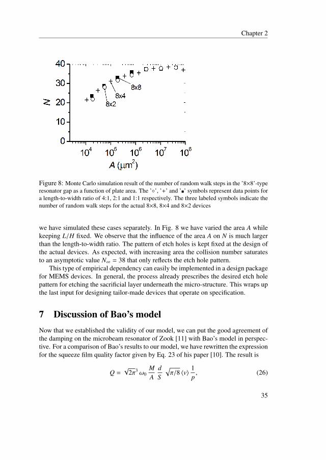
Figure 8: Monte Carlo simulation result of the number of random walk steps in the ’8×8’-typeresonator gap as a function of plate area. The ’◦’, ’+’ and ’�’ symbols represent data points fora length-to-width ratio of 4:1, 2:1 and 1:1 respectively. The three labeled symbols indicate thenumber of random walk steps for the actual 8×8, 8×4 and 8×2 devices
we have simulated these cases separately. In Fig. 8 we have varied the area A whilekeeping L/H fixed. We observe that the influence of the area A on N is much largerthan the length-to-width ratio. The pattern of etch holes is kept fixed at the design ofthe actual devices. As expected, with increasing area the collision number saturatesto an asymptotic value N∞ = 38 that only reflects the etch hole pattern.
This type of empirical dependency can easily be implemented in a design packagefor MEMS devices. In general, the process already prescribes the desired etch holepattern for etching the sacrificial layer underneath the micro-structure. This wraps upthe last input for designing tailor-made devices that operate on specification.
7 Discussion of Bao’s modelNow that we established the validity of our model, we can put the good agreement ofthe damping on the microbeam resonator of Zook [11] with Bao’s model in perspec-tive. For a comparison of Bao’s results to our model, we have rewritten the expressionfor the squeeze film quality factor given by Eq. 23 of his paper [10]. The result is
Q =√
2π3 ω0MA
dS
√π/8 〈v〉 1
p, (26)
35
Chapter 2
where plate mass is defined by M = ρ A t and ρ, t and S (in the notation used by Bao)represent density of plate material, plate thickness and circumference of plate area A,respectively. Using
β =d
dpb =
ddp
(Mω0
Q
), (27)
the expression for βBao takes the shape
βBao =Ad
Sπ2 〈v〉 =
Ad
2 (L + H)π2 〈v〉 , (28)
Our result reads
βSuijlen =Ad
τ
1 + (ω0 τ)2 (29)
where the diffusion time τ is determined by random walk Monte Carlo simulationsfor a plate with area A = L×H, with L and H the plate length and width, respectively.The diffusion time τ scales as
τ ∝ (d 〈v〉)−1 (30)
as follows from the collision number N ∝ d−2 (Eq. (19)) and the gap crossing time〈τ1〉 ∝ d/〈v〉 (Eq. (18)). The dependence on the plate geometry in the Monte Carlosimulations can be approximated by
τ ∝ [min(L,H)
]1.6. (31)
The latter can be understood readily when realizing that the smallest dimension ofthe plate will determine the escape probability for the molecules in the gap volume.The 1.6 power dependence is due to the non-Gaussian distribution function for thesingle step displacement in Eq. (25).
By combining the results of Eqs. (28), (29), (30) and (31), we find
βSuijlen
βBao≡ η ∝
[min(L,H)
]1.6
2(L + H) d, (32)
depending only on the geometry of the device.In Tab. 4 we compare both models for the microbeam of Zook and three plate os-
cillators with dimensions corresponding to the devices in section 4, however, withoutthe etch holes. We see a fair agreement between both models for Zook’s device andrapidly increasing factors of disagreement for the larger devices. This is no surprisegiven the very different scaling rules for the dimensions of the devices as discussedabove.
36
Chapter 2
Table 4: Comparison of β values, calculated with the models of Bao (Eq. (28)) andSuijlen (Eq. (29)). Here the η values are defined by the ratio βSuijlen/βBao (Eq. (32)).The size of the test samples corresponds to the 8×2, 8×4 and 8×8 devices specifiedin section 4. However, the models have been applied to a plate without etch holes.
Test sample L × H ω0/(2π) d βSuijlen βBao η(no etch holes) (µm2) (kHz) (µm) (10−6 kg/s mbar)
We have introduced an analytical model for squeeze film damping of an oscillatingplate in the regime of free molecular flow. This model is based on the increase indensity due to the amplitude of the plate movement. A phase shift due to the counter-acting random walk diffusion in the gap which tries to equalize this increase, resultsin an extra damping that agrees well with accurate experimental results. The calcula-tion of the random walk diffusion time is based on the well known properties of freemolecular flow and the interaction of gas molecules with a surface at conditions rep-resentative for MEMS operation. Full thermal accommodation is the rule; specularreflection is the exception in all practical cases. Through the model we have gainedinsight which allows us to design tailor-made devices that will operate on specifica-tion.
A Molecular impingement rate
In kinetic theory molecular transport is solely determined by the velocities and colli-sions of the individual molecules. Because these velocities have random values as aconsequence of the collisions, only the velocity-averaged value according to a certainprobability distribution can be regarded. This probability distribution is known as thenormalized velocity distribution PMB of Maxwell-Boltzmann. In spherical coordi-
37
Chapter 2
nates it is formulated as
PMB(v, θ, φ) dvdθdφ = PV (v)dv PΘ(θ)dθ PΦ(φ)dφ,
PV (v)dv =4 v2
√πα3
e−(v/α)2dv,
PΘ(θ)dθ =12
sin θ dθ,
PΦ(φ)dφ =1
2πdφ,
(33)
and gives the fraction of the gas molecules having speeds between v and v + dv,traveling in a solid angle element between (θ, φ) and (θ + dθ, φ + dφ). The threeindividual probability distributions for v, θ and φ are normalized in the domains v ∈[0,∞), θ ∈ [0, π) and φ ∈ [0, 2π). The characteristic speed α is defined by
α =√
2kB T/m (34)
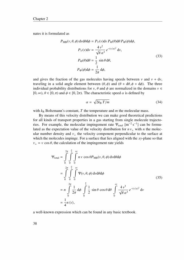
with kB Boltzmann’s constant, T the temperature and m the molecular mass.By means of this velocity distribution we can make good theoretical predictions
for all kinds of transport properties in a gas starting from single molecule trajecto-ries. For example, the molecular impingement rate Ψtotal [m−2 s−1] can be formu-lated as the expectation value of the velocity distribution for n v⊥ with n the molec-ular number density and v⊥ the velocity component perpendicular to the surface atwhich the molecules impinge. For a surface that lies aligned with the xy-plane so thatv⊥ = v cos θ, the calculation of the impingement rate yields
Ψtotal =
2π∫
0
π2∫
0
∞∫
0
n v cos θPMB(v, θ, φ) dvdθdφ
=
2π∫
0
π2∫
0
∞∫
0
Ψ(v, θ, φ) dvdθdφ
= n
2π∫
0
12π
dφ
π2∫
0
12
sin θ cos θ dθ
∞∫
0
4 v3
√πα3
e−(v/α)2dv
=14
n 〈v〉,
(35)
a well-known expression which can be found in any basic textbook.
38
Chapter 2
Also the pressure on the wall can be calculated as the expectation value of Eq.(33) for (n v⊥) · (2m ∆v⊥). The first term describes the contributing incident flux andthe second term the momentum transferred on collision with the wall. The knownresult reads p = 1
3 n m 〈v2〉 likewise expressed as p = n kB T , being Boyle’s law.Important in this respect of molecules interacting with a wall is the flux-weighted
speed distribution Pwall which is in terms of PMB defined as:
Pwall =n v⊥Ψtotal
PMB (36)
Again supposing the wall surface to be aligned with the xy-plane and using the current(v, θ, φ)-coordinates, this distribution is written as
Pwall dvdθdφ = PwallV (v)dv Pwall
Θ (θ)dθ PwallΦ (φ)dφ,
PwallV (v)dv = 2
v3
α4 e−(v/α)2dv,
PwallΘ (θ)dθ = 2 sin θ cos θ dθ,
PwallΦ (φ)dφ =
12π
dφ,
(37)
The two individual probability distributions PwallV (v)dv for v and Pwall
Φ(φ)dφ for φ are
normalized here in the same domains as their equivalents in PMB. However forPwall
Θ(θ)dθ the domain is restricted to θ ∈ [0, π/2). A comparison of the individual
probability distributions to their equivalents in PMB leads to the next relations whichcan be helpful:
PwallV (v) =
√π
2vα
PV (v) (38)
PwallΘ (θ) = 4 cos θ PΘ(θ) (39)
PwallΦ (φ) = PΦ(φ) (40)
If the application features planar symmetry, calculations become simpler withcartesian coordinates vx, vy and vz. In that case the flux-weighted speed distributionis formulated as
Pwall dvxdvydvz = Pwallvx (vx)dvx Pwall
vy (vy)dvy Pwallvz (vz)dvz,
Pwallvx (vx)dvx = (α
√π)−1 e−(vx/α)2
dvx,
Pwallvy (vy)dvy = (α
√π)−1 e−(vy/α)2
dvy,
Pwallvz (vz)dvz = 2
vz
α2 e−(vz/α)2dvz.
(41)
39
Chapter 2
Here the distributions for vx and vy represent identical Normal distributions with vari-ance σ2 = α2/2 = (π/8)〈v〉2 and the domains of vx and vy both span the whole realline (−∞,∞). The distribution for vz represents a Rayleigh distribution with parame-ter α/
√2 where the vz-domain contains only the half real line [0,∞).
B Distribution of step length r1
With the establishment of the flux-weighted velocity distribution of Eq. (37), theprobability distribution P(r1)dr1 of the random-walk step-length r1 is easily derivedusing the relation
r1 = d tan θ. (42)
The random variable θ in this situation has the marginal distribution PwallΘ
(θ) dθ. Re-calling basic probability theory, the distribution PY dy of any other variable y, de-pending on θ according to an invertible and differentiable transformation f (θ), willsatisfy
PY (y) dy = PwallΘ
(f −1(y)
) ddy
f −1(y) dy, (43)
where f −1 represents the inverse transformation.Identifying arctan(r1/d) as the f −1(y) in our case from Eq. (42), the distribution
function P(r1)dr1 of step length r1 is found to be
P(r1) dr1 = PwallΘ
(arctan(r1/d)
) ddr1
arctan(r1/d) dr1
= 2r1/d
1 + (r1/d)2
1/d1 + (r1/d)2 dr1
=2d2 r1
(r21 + d2)2
dr1
(44)
References[1] J.J. Blech, J. Lubr. Technol. 105 (1983) 615-20.
[2] T. Veijola, H. Kuisma, J. Lahdenpera, and T. Ryhanen, Sens. Actuators A 48(1995) 239-48.
[3] M. Bao, H. Yang, Sens. Actuators A 136 (2007) 3-27.
[4] G. Li and H. Hughes, Proc. SPIE 4176 (2000) 30-46.
40
Chapter 2
[5] W. Newell, Science 161 (1968) 1320-6.
[6] Y. Kawamura, K. Sato, T. Terasawa, and S. Tanaka, Proc. Transducers’87 (1987)283-6.
[7] Z. Kadar, W. Kindt, A. Bossche, and J. Mollinger, Proc. Transducers’95 (1995)29-32.
[8] B. Li, H. Wu, C. Zhu, and J. Liu, Sens. Actuators A 77 (1999) 191-4.
[9] H. Sumali, J. Micromech. Microeng. 17 (2007) 2231-2240.
[10] M. Bao, H. Yang, H. Yin, Y. Sun, J. Micromech. Microeng. 12 (2002) 341-346.
[11] J. Zook, D. Burns, H. Guckel, J. Sniegowski, R. Engelstad, Z. Feng, Sens. Ac-tuators A 35 (1992) 51-59.
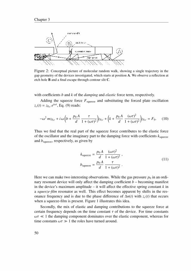
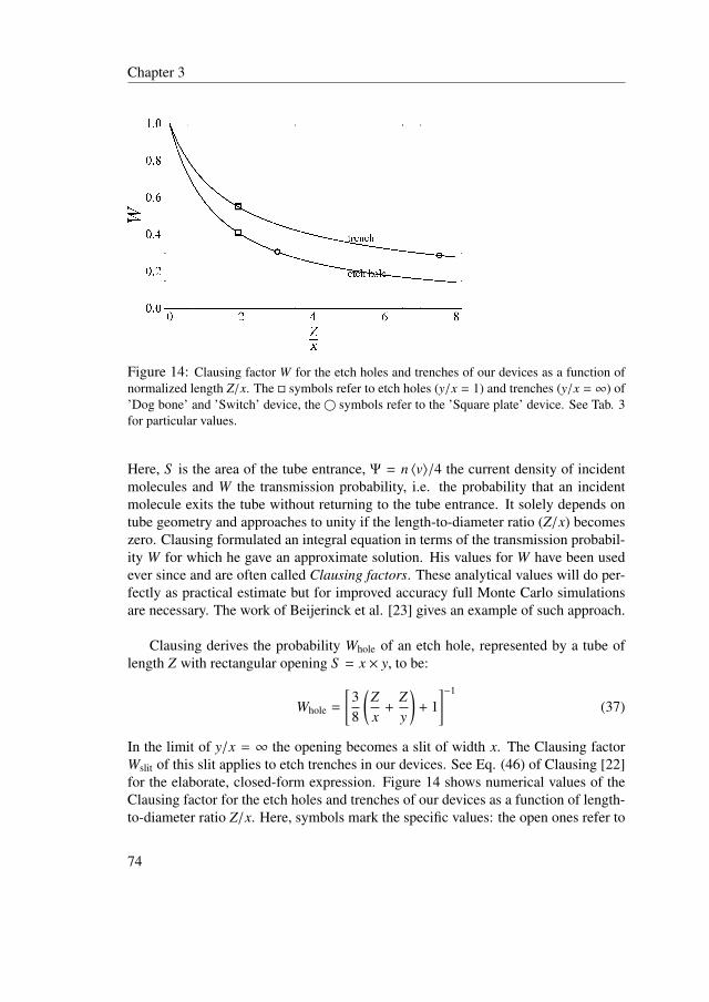
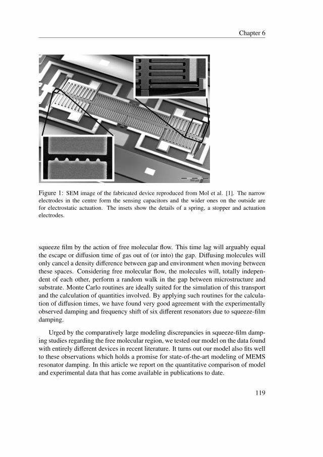
Micro-mechanical resonators are known to require vacuum conditions forproper operation, involving free molecular flow of the residual gas in the squeeze-film box under the resonator. This flow is ideally suited to be described byinvestigating trajectories of the individual molecules using a Monte Carlo ap-proach. We developed a simple analytical model for describing squeeze-filmforces on MEMS resonators, with the average escape time τ of a molecule fromthe squeeze-film box as the only device-based free parameter. The value of τ iscalculated using a Test Particle Monte Carlo Method (TPMC). Geometrical de-tails of the MEMS resonator including etch holes and slits can be readily accom-modated in TPMC routines, in contrast to the rather laborious implementationof these details in case of a continuum description. Using the model, three dif-ferent MEMS resonators have been designed and fabricated for an application aspressure sensors. Each device can be read-out by monitoring either the increasein damping or the shift in resonant frequency. The experimentally observed be-havior of the devices in both read-out modes is fully consistent with the model,showing agreement to within 10%.
1 IntroductionThe advent of microfabrication technologies in the last couple of decades has led toan exciting and revolutionary field called micro-electro-mechanical systems (MEMS)technology. MEMS applications are found in all kinds of sensors and actuators con-tained by modern cars and everyday digital electronics. Their development requiresextensive knowledge on the behavior of the mechanical element in the system. Ex-cept structural mechanical properties, influences from outside must be considered todescribe the element’s motion correctly. In particular the role of gas damping on theelement is important. For a resonant sensor which needs high resolution, dampingshould be minimized to enhance quality factor. With regard to the outright narrowgaps between element and electrodes featuring typical designs, a single phenomenonappears to be dominant: squeeze-film damping.
In MEMS resonators the narrowly separated surfaces of movable elements canconfine the gas almost completely in the gap while compressing the film in an os-cillation cycle, even though the structure is open at the ends. This represents oneextreme of the squeeze-film effect: the compression of a gas between approachingparallel surfaces with a gap much smaller than their dimensions. Since the gas cannotescape, the dominant force is one of compression and this adds to the structure’s stiff-ness, raising its resonance frequency. Only at low frequencies, as the gas is pushedout of and drawn back into the gap, the gas-resonator interaction obtains a pure dragcharacter.
44
Chapter 3
Because the gases trapped in the cavities of MEMS often are so rarefied thatthe molecular mean free path exceeds the gap dimensions by at least an order ofmagnitude, the squeeze-film flow becomes ’free molecular’. Squeeze-film dampingin this regime is an interesting problem that has been attracting a lot of attentionin the last decade. Its modeling has long been retained to the field of continuumflow, using an effective viscosity µeff that takes into account the rarefaction effects[1, 2, 3]. Although this approach can predict both damping and frequency shift of theresonator due to film flow, its application to complex geometrical structures in real-life technology – including etch holes, springs and stacked structures – is impossiblewithout a highly specialized and tedious programming effort.
Here, a molecular approach to directly model the transport of individual moleculesshows a great advantage. Because the molecules do not interact with each other,molecular trajectories in the system consist of randomly oriented straight line pas-sages between structural boundaries. The (numerical) simulation of these trajectoriescan be carried out in a direct manner and easily be applied to large trajectory num-bers for an accurate picture of gas flow. Currently this so called Test Particle MonteCarlo (TPMC) method has been developed to a powerful means in solving molecularflow in complex vacuum systems [4].
Early applications of molecular transport [5, 6, 7, 8, 9], however, assumed freespace kinetics for squeeze-film damping modeling, ignoring with it the constrainedtrajectories that the molecules in the narrow resonator gaps are performing. Con-sequently, these models effectively give account of the kinetic damping contribu-tion only, underestimating the experimental values for squeeze film damping largely[10, 11].
More recent applications [11, 12, 13, 14, 15] do consider the confined space of theresonator gaps and approximate reasonably well the experimental values of qualityfactor due to squeeze-film damping. One important aspect, however, is being ignored:the compressibility of the squeeze-film. A clue for this aspect is given by the phe-nomenon in resonators that resonance frequency increases with increasing ambientpressure (Fig. 1). Andrews et al. [16] have performed measurements on a devicewith such a pronounced containment of the gas in the squeeze-film box that this phe-nomenon starts playing a role at pressures where the film flow is still free molecular.
For this reason we developed a simple analytical model for squeeze-film damp-ing in the regime of free molecular flow, which is able to predict the damping forcecomponent degrading the resonator’s quality factor as well as the spring force com-ponent that raises the resonance frequency. We apply this model to measurements onthree different MEMS resonators to show good agreement in the effect of squeeze-film damping on quality factor and resonance frequency. The only free parameter isthe device-based average escape time τ of gas molecules from the squeeze-film box.Based on the model, we have designed and fabricated three MEMS resonators that
45
Chapter 3
Figure 1: Resonance spectrum of a squeeze-film resonator at constant driving force F0. Withincreasing pressure p the amplitude X at resonance decreases, the width of the resonance in-creases (both due to the increased damping), and the resonance frequency ω0 shifts to higherfrequencies.
can serve as pressure sensors. Pressure read-out can be done either by monitoring theincrease in damping or the shift in operating frequency. The experimental results inboth read-out modes are consistent with the model predictions, within an accuracy oftypically 10%. This demonstrates the value of the model for designing new devices,avoiding trial and error loops to meet the specifications.
In section 2 we discuss the model in detail. The calculation of the escape timeτ is discussed in section 3. Also we apply our model to predict the damping of oneof the devices of Legtenberg et al. [17], which has also been used by Leung et al.[15] to validate their Monte Carlo approach for calculating the damping coefficient.In section 4 we present the devices that have been designed and fabricated, includingthe results obtained by simulation of the mechanical behavior with COMSOL Mul-tiphysics. In section 5 the experimental results are shown, including a discussion ofthe analysis of the raw data on the resonance profiles. To represent the experimentalresults of all devices in a single diagram, we introduce a generalized two-dimensionalplot in section 6 with scaled values of the pressure-dependency of both damping andfrequency shift as major axes. Finally, in section 7, we present some concludingremarks on the lessons learned.
46
Chapter 3
2 Squeeze-film damping in free molecular flowThe basics are rather simple: due to the oscillation of the resonator according toz0(x, y) sin(ω t), the number density n in the ’box’ between resonator and the fixedsubstrate will vary proportional to sin(ω t + φ). The driving force for the variation ofthe density is the varying height of the gap
d(x, y; t) = d + z(x, y; t) = d + z0(x, y) sin(ω t). (1)
In a macroscopic picture, this change in height results in an increase in volume andthus a decrease in number density. In a microscopic picture, the change in heightresults in an increase in the round-trip time of the colliding molecules and thus in adecrease of the wall collision rate which indicates a decrease in number density. Thephase difference φ in the response of the density n reflects the time lag in the freemolecular flow equalizing the number density to its value n0 outside the squeeze-filmbox. If we denote the response time for this process as τ, we can define two regimesin terms of the value of the non-dimensional characteristic parameter ωτ.
First, for ωτ � 1, the density will be nearly fully determined by the change ingap height and the influence of free molecular flow that equalizes the pressure is verysmall. As a result, the phase difference will be close to zero; φ ≈ 0. The increasein density is then nearly out of phase with the velocity of the resonator. The productof change in density and work done by the resonator on the gas then averages out toapproximately zero over one period of oscillation. We then observe a small value ofthe damping; the major effect is on the effective force constant of the resonator whichincreases due to the ’air cushion’. This situation can be compared to a person tryingto get the air out of an air mattress by jumping up and down on it. The bounce isperfect, but very little air escapes.
Second, for ωτ � 1, the change in number density will be rapidly equalized bythe free molecular flow. For this reason, the effective variation of the density willbe much less than predicted by the changes in volume or round-trip time betweentwo collisions, whatever picture is preferred. The phase shift in the number densityis given by φ ≈ π/2 and is in phase with the velocity of the resonator. Under theseconditions, damping dominates and the increase in the effective force constant (orstiffness) of the resonator is rather small. Returning to our example of an air mattress,this situation corresponds to sitting down on it and letting the air flow out: no bounce,but a lot of air escapes!
2.1 Model assumptionsFor industrial applications, we are interested in an efficient model that describes bothdamping and frequency shift for optimizing the design of MEMS devices. We do
47
Chapter 3
not aim at including all detail, but search for a trade-off between insight based on ananalytical description, sufficient accuracy, flexibility in incorporating new geometries,and rapid numerical characterization in a design code. This implies that we will onlyinclude effects that are first-order in the amplitude of the oscillating plate; all higher-order terms will be discarded. This approach differs from most papers published inthis field, where the emphasis is put on achieving ultimate accuracy by including allpossible terms.
Because molecules in the squeeze-film box do not interact with each other, theymove in and out of the box only via random crossings between facing boundaries ofresonator and substrate. This transport occurs independent of local density differencesinside the film. We characterize this transport by the ensemble-averaged escape timeτ(x, y). For the correct process of averaging, Boltzmann statistics of the gas are takeninto account. For all devices with a lateral dimension much larger than the gap height,the escape time τ(x, y) will hardly depend on the location (x, y) in the squeeze-filmbox. For devices with a large set of equally spaced etch holes, this will even be morepronounced. Therefore, we will use a spatially averaged value of the escape time, asgiven by
τ =
"
Sτ(x, y) dxdy
/"
Sdxdy , (2)
with S referring to the lateral domain of the squeeze-film box in x- and y-coordinates.This assumption also implies that a density profile n(x, y; t) will decay with a singletime constant equal to the spatially averaged escape time τ, allowing us to use thespatially-averaged value n(t) of the density:
n(t) =
"
Sn(x, y; t) dxdy
/"
Sdxdy . (3)
The value of τ will depend on the geometrical details of the device, such as gapheight, area, and etch holes in the plate. However, these assumptions imply that themode shape z(x, y; t) does not have any influence on the dynamics of the gas in thesqueeze-film box. At a later stage, where we present the results for the calculation ofτ, we will discuss the validity of these approximations.
For our model we choose the equilibrium values n0 and T0 of the surroundinggas outside the box as a reference for density and temperature, respectively. Theincrease ∆n(t) = n(t) − n0 in density of the gas in the squeeze-film box is the drivingforce for damping and the increase in the elastic force constant. We introduce themode-averaged value zc,0 of the amplitude
z0,c =
"
Cz0(x, y) dxdy
/"
Cdxdy , (4)
48
Chapter 3
– with C denoting the domain in x, y space of our deflected microstructure –, to de-scribe this driving force.
2.2 Analytical solutionThe time dependent contribution ∆n(t) to the density in the squeeze-film box is gov-erned by the simple differential equation
ddt
∆n(t) = −n0ddt
(zc(t)
d
)− ∆n(t)
τ, (5)
where the first term on the right is the driving force leading the system from equilib-rium and the second term represents the relaxation of the system back to equilibriumby the kinetics of free molecular flow. Please note that zc is defined as pointing up-ward, out of the squeeze-film box. These equations indeed neglect higher order termsin the displacement zc(t). In the driving force we use the equilibrium density n0 aspre-factor because the time derivative contains the zc-dependency. In the relaxationterm the increase ∆n is first order in zc which allows us to use the time- and space-averaged value of the escape time τ.
Assuming a forced plate oscillation zc(t) = z0,c eiωt according to Eqs. (4) and (1)and a trial solution ∆n(t) = ∆n0 eiωt with a complex-valued amplitude ∆n0 we find
∆n(t) = −n0
diωτ
1 + iωτzc(t) . (6)
Assuming that the fluctuations of number density n due to plate oscillation zc areisothermal, the force of the squeeze-film on the resonator plate Fsqueeze is readilyderived from simple gas kinetics as given by the law of Boyle-Gay Lussac:
Fsqueeze(t) = ∆n(t) kB T0 A, (7)
The assumption of an isothermal temperature T0 is fully justified, because the productof the modulation ∆n(t) in density and a possible non-isothermal contribution to thetemperature would result in higher-order terms in zc. Applying Eq. (6), the squeezeforce reads:
Fsqueeze(t) = − p0 Ad
iωτ1 + iωτ
zc(t) . (8)
The effect of this complex-valued force on the oscillating plate can be understood byconsidering the classical model for the motion of a forced harmonic oscillator, givenas a differential equation in the center-of-mass plate displacement zc(t),
mzc + bzc + kzc = F0 eiωt, (9)
49
Chapter 3
Figure 2: Conceptual picture of molecular random walk, showing a single trajectory in thegap geometry of the devices investigated, which starts at position A. We observe a reflection atetch hole B and a final escape through contour slit C.
with coefficients b and k of the damping and elastic force term, respectively.Adding the squeeze force Fsqueeze and substituting the forced plate oscillation
zc(t) = z0,c eiωt, Eq. (9) reads:
−ω2 mz0,c + iω(b +
p0 Ad
τ
1 + (ωτ)2
)z0,c +
(k +
p0 Ad
(ωτ)2
1 + (ωτ)2
)z0,c = F0. (10)
Thus we find that the real part of the squeeze force contributes to the elastic forceof the oscillator and the imaginary part to the damping force with coefficients ksqueezeand bsqueeze, respectively, as given by
ksqueeze =p0 A
d(ωτ)2
1 + (ωτ)2 ,
bsqueeze =p0 A
dτ
1 + (ωτ)2 .
(11)
Here we can make two interesting observations. While the gas pressure p0 in an ordi-nary resonant device will only affect the damping coefficient b – becoming manifestin the device’s maximum amplitude – it will affect the effective spring constant k ina squeeze-film resonator as well. This effect becomes apparent by shifts in the res-onance frequency and is due to the phase difference of ∆n(t) with zc(t) that occurswhen a squeeze-film is present. Figure 1 illustrates this idea.
Secondly, the mix of elastic and damping contributions to the squeeze force atcertain frequency depends on the time constant τ of the device. For time constantsωτ � 1 the damping component dominates over the elastic component, whereas fortime constants ωτ � 1 the roles have turned around.
50
Chapter 3
3 Determination of time constant τ
3.1 Model calculation
Because the molecules in the squeeze-film box do not interact with each other, theywill perform independent random walks in the squeeze-film box (Fig. 2). Collisionswill only take place with the gap boundaries, i.e. resonator plate, substrate surfaceand the adjacent sides. In this way straight-line, randomly oriented gap-crossingsof the molecules link together to form random walk trajectories between a randomstarting point in the gap space and an escape at openings like gap boundary and plateperforations. For a large sample of molecules randomly initiated in the gap space,normalized distribution functions for all sorts of trajectory parameters can be derivedshowing the collective behavior of molecules in the squeeze-film flow.
In our TPMC approach, we use a routine that initializes the trajectories uniformlyin the gap space, by choosing three random numbers x0 ∈ [0, Lb], y0 ∈ [0,Hb] andz0 ∈ [0, d] for the Cartesian coordinates of the initial position. Because we assumethat the gas is in thermal equilibrium, Boltzmann statistics determine the initializedvelocity vector of each molecule. Simple procedures are available for choosing ran-dom values of the Cartesian components vx, vy and vz of this velocity, because Boltz-mann statistics are governed by a Normal distribution for all components, with vari-ance σ2 = (π/8)〈v〉2 and 〈v〉 =
√8kBT/(πm) the average velocity of the molecule.
With regard to the closed edges of the device gap, the diffusing molecules are sim-ulated along their trajectory in a box bounded by a surface plane coinciding with thebottom of the moving plate, by the substrate surface and the edges of the 1.0 µm-thickburied oxide layer. Because of etch holes and the contour slit of the moving plate,the molecule eventually escapes from this box, ending its tracking. The etch holesand contour slits resemble narrow tubes and trenches, giving incident molecules onlya limited probability for escaping. This transmission probability can be determinedanalytically for different geometries and is known as the Clausing factor (App. A).A visualization of this phenomenon is shown in Fig. 2 in which we have schemati-cally drawn the random walk of a single molecule bouncing up and down in the gap,attempting to escape. Although the molecule at a certain moment enters an etch hole,it does not escape in this case: it experiences a few bounces on the wall of the holeand is finally reflected back into the gap.
The displacement vector ~s j for the jth wall-to-wall flight is found by projectingthe initial position along the velocity vector on the appropriate box plane. The routineselects the boundary plane of the actual collision according to the direction of thegiven velocity and the distance from the center of the gap space (App. B). At the newposition on the destination plane, the velocity vector is updated with random values
51
Chapter 3
Figure 3: TPMC method for diffusion time calculation of the ’Switch’ device. Trajectoriesof 80 molecules are simulated to begin at random positions inside the box-shaped gap andterminate on escape through the resonator contour slit and etch holes, respectively. The solidsquare denotes the ’Switch’ resonator plate above the gap.
52
Chapter 3
0.1 1 10 100 1000 104100
120
140
160
180
200
ΗA
N
Figure 4: Monte Carlo simulations of the collision number N in a square-contoured gap withfeatures according to that of the ’Switch’ resonator (Tab. 3). The data points show the increaseover scaled gap footprint ηA.
from a flux-weighted Maxwell distribution (see also appendix A of chapter 2). Again,a simple transformation allows for an easy pick of a random value.
After each collision we assign new, random values to the velocity vector (vx, vy, vz)of the molecule and check if the point of impact coincides with an etch hole or slit:
• if not, we continue the current trajectory;
• if so, we either store the value of the collision number Ni and the accumulatedescape time τd,i and initialize a new trajectory (i + 1) or continue the currenttrajectory according to the result of a random draw accounting for the Clausingfactor.
In figure 3 we have plotted the trajectories of eighty molecules for the ’Switch’ device.We see that most particles leave the squeeze-box through the etch holes in the plate.Furthermore, we observe the characteristic behavior of local random walk interruptedby surprisingly long jumps, as determined by the asymptotic behavior ∼ 1/r1 of thedistribution function for the displacement r1 in a single crossing between top andbottom of the squeeze-box (or vice versa).
We do not consider molecules wandering off in the gap region outside the con-tours of the device plates: in our procedure, we use a gap that is simply framed bythe rectangular shape of the plates. This simplification, to prevent the more tedious
53
Chapter 3
Table 1: Results of the time constants τfit, τsum and τ1/e for the three resonatorsinvestigated. Additionally the values of the parameters α and λ for the curve-fittedgamma functions through the Monte Carlo results for P(τd) are listed. The numbersbetween parentheses denote the fractional difference in value as compared to τsum.
collision-site detection around springs and anchors, is fully justified for our devicesthat are riddled with etch holes.
Simulations in a square-contoured gap with features of the resonators investigated(see ’Switch’ Tab. 3) show that the collision number N hardly increases with thescaled value ηA = L2/L2
Switch of the area of the device, with L a measure for the lateralextent. Numerical results are shown in Fig. 4. In the operational point ηA = 1, thedependency can be linearized to
ηA = 1 : dN/N = 0.11 dηA/ηA (12)
A 20% increase in plate area results in only 2% extra collisions of a molecule toescape from the gap, with a correspondingly small increase of the escape time. Thisis well within the systematic error of our analytical model due to its simplifications.
The routine developed in this way, was written and run in Mathematica1 to pro-duce graphics and statistical output in a user-friendly manner. Besides escape time τd
and collision number N, the procedure also stores other properties of the trajectoryto investigate the diffusion process such as accumulated path length S =
∑Nj |~s j| or
average wall-to-wall flight time 〈τflight〉 = 1N
∑Nj τflight, j and is repeated to improve
statistical accuracy in these parameters.On our system (x86, Intel Xeon, 64 bit) the calculation for a sample of n = 105
trajectories in the resonator gap (typically N = 150 collisions) takes ten minutes,which is fast enough for implementation in a MEMS design code. We have checkedthat the variance in the sample mean τ = 〈τd〉 in different sample runs (each withn = 105 trajectories) follows the expected behavior according to σ2
τ ∝ 1/n.
1Version 7 by Wolfram Research Inc., UK
54
Chapter 3
Figure 5: Normalized distribution function P(τd) for the escape time τd for the ’Switch’resonator investigated in this paper.
3.2 Escape-time distribution functionIn figure 5 we show the Monte Carlo result for the normalized distribution functionP(τd) for the escape time τd for the ’Switch’ resonator investigated in this paper. Thedeviations from a smooth curve are significant and not the result of stochastic noisedue to a finite sample size. The data points have been averaged by using a 0.1 µstime-bin. The solid line represents a least-squares curve-fit with the gamma densityfunction Γ(t;α, λ).
The distribution function P(τd) is the input to determine the time constant τ asintroduced in Eq. (5). Solving this equation without the external term due to the platemotion, we find a solution
∆n(t) = ∆n(0) exp(−t/τ), (13)
showing a simple exponential decay of the initial deviation ∆n(0) of the density insidethe gap from its equilibrium value n0 outside the gap. The remnant particle fractionζ(t) = ∆n(t)/∆n(0) directly derives from P(τd) if we start summing up the escapefrequencies from τd = 0 to τd = t and subtract the total from 1, as given by
ζ(t) = 1 −t∫
0
P(τd) dτd . (14)
The shape of this particle fraction for the ’Switch’ device resembles an exponentialfunction with a single time constant that can be determined from either the 1/e decaypoint or the average value. Due to the deviations of P(τd) from the simple exponential,
55
Chapter 3
however, we have to carefully investigate the most appropriate method to derive thetime constant τ in Eq. (5) from this distribution function. We now discuss threedifferent recipes to determine the value of τ. The variance in the outcome of thesedifferent methods will provide us with an indication of the accuracy of the value of τ.
First, we apply a method that takes into account the shape of P(τd), by performinga least squares curve-fit of P(τd) with the gamma density function Γ(t;α, λ) withα > 0 and λ > 0. The result of this curve-fit is given in Fig. 5. We observe a fairlygood description of P(τd), apart from the extra wiggles that are specific for the device.The average value for the time constant based on this curve-fit is given by
τfit = α/λ. (15)
We observe that for the ’Switch’ device the Gamma function overestimates the dis-tribution for large values of the escape time, which will result in too large values ofτfit.
Next, we calculate τ by straight-forward averaging of the discrete results forP(τd), as given by
τsum =
∞∑
i=0
τd,i P(τd,i) (16)
over all time bins with index i. This last method takes into account all details of theMonte Carlo results, which cancels the errors introduced by using a curve-fit.
Finally, to connect to the analytical solution of the homogeneous solution of Eq.(5), we determine τ by solving
ζ(τ1/e) = 1/e , (17)
which neglects details of the specific shape of the distribution function P(τd). This isa rather simple choice which (1) puts most emphasis on the high frequency end of thedistribution function and (2) is sensitive to details of the distribution function such asthe observed wiggles and is sensitive to the shot-noise involved.
The results for the time constant τ of these three recipes are compiled in Tab. 1, forall three devices investigated in this paper. We see that the different time constantshave quite similar values. The differences between τfit and τsum correlate with anunderestimation (’Dog-bone’, ’Square plate’) or an overestimation (’Switch’) of theMonte Carlo data by the curve-fit, respectively. This same behavior is also reflectedin the results for τ1/e: an underestimation of the tail for long escape times correspondsto a faster decay at short times, resulting in a smaller value of the time constant τ1/eand vice versa. The calculation of the average value τsum directly from the MonteCarlo results of the distribution function P(τd) takes into account all details of the
56
Chapter 3
Table 2: Experimental squeeze-film damping coefficient bsqueeze at p = 1 Torr of the ”310 µm-nocap” device as measured by Legtenberg et al. [17], in comparison to the calculated resultsof Leung et al. and the results of our fast-prototyping TPMC approach. The number betweenparentheses indicates the error in the last digit.
Property Definition Value
Material SiliconDensity ρ (103 kg/m3) 2.33Plate area Aplate (µm2) 310 × 100Plate thickness D (µm) 1.5Gap width d (µm) 1.18
Effective mass m (µg) 0.11Resonance fre-quency ω0/(2π) (kHz) 163Quality factor Q 71(4)
specific device. For this reason it is our time constant of preference. In this paper wewill use
τ ≡ τsum (18)
when referring to a calculated result for the time constant.
3.3 Test of TPMC method
As a test of our TPMC routine we have calculated the squeeze-film damping coeffi-cient bsqueeze of the ”310 µm -no cap” device of Legtenberg et al. [17] at p = 1 Torr.We compare this value to the experimental value derived from Legtenberg’s Q vs. pplot. Because we are in the pressure range far from the low pressure region featuring
57
Chapter 3
Figure 6: Cross section of SOI resonators investigated.
Q values constant with pressure, damping is gas dominated and we may use:
bsqueeze,expt ' bexpt − bkin ,
=mω0
Q− 16 Aplate
π 〈v〉 · 1 Torr(19)
with m = ρ Aplate D as the effective resonator mass and bkin as the kinetic dampingcontribution according to Christian [18]. Table 2 lists the device properties and mod-eling results. The error margin of the quality factor stems from extracting it fromthe plot. The error margin of the modeled squeeze damping coefficient follows fromthe range of possible time constants, formed by the values of τfit, τsum and τ1/e asdescribed in the previous section.
Finding good agreement of our model outcome with the experimental dampingvalue, we assume our TPMC method to be valid.
4 DevicesWe test our model on the basis of experimental data on three distinct uncapped res-onators. The resonators are produced on a Silicon-On-Insulator (SOI) substrate usingsurface micro-machining. Contours of the structures are patterned onto the substrateand etched through the top silicon layer, cutting out the resonator features. To facili-tate the wet etch of the 1.0 µm intermediate oxide layer, all plates and wide beams areperforated with l× l sized holes in a h× h spaced grid. Thus a free-standing structureresults, with a gap distance to the substrate d = 1.0 µm (Fig. 6). The devices are la-beled ’Dog bone’, ’Square plate’ and ’Switch’ and operated in out-of-plane resonantmodes subjected to squeeze-film damping in the gap between resonator and substrate.Characteristic dimensions are given in Tab. 3.
Mode shapes and resonance frequencies of the respective designs were deter-
58
Chapter 3
Table 3: Characteristic parameters of the three MEMS devices. Resonance frequencyω0,mat and spring constant kmat as calculated from a finite-element simulation usingCOMSOL. Value of τ according to TPMC calculation.
Property Definition Dog bone Square plate Switch
Gap frame Lb × Hb (µm2) 112 × 62 172 × 172 172 × 172Gap width d (µm) 1.0 1.0 1.0Unit cell size h × h (µm2) 7.0 × 7.0 9.0 × 9.0 7.0 × 7.0Etch hole size l × l (µm2) 0.8 × 0.8 0.5 × 0.5 0.8 × 0.8Trench width w (µm) 0.8 0.2 0.8
Plate area A L × H (µm2) 100 × 50 160 × 160 160 × 160Plate thickness D (µm) 1.5 1.5 1.5Spring length s (µm) 18 18 50Spring width t (µm) 16 4 10
Figure 7: Mode shapes and strain energy volume distribution of the resonator structures in-vestigated. The etch holes present in the real devices were omitted to facilitate meshing for theFEM simulations.
60
Chapter 3
mined from finite-element (FEM) simulations using COMSOL Multiphysics2. As-suming quality factors in the usual range (Q > 10), these resonance frequencies willshow a perfect match with the corresponding eigenfrequencies ω0,mat. Thus, for eachdesign, an eigenfrequency analysis was setup for simulation of the lowest bendingmode resonance. For unproblematic meshing of the domains the etch holes in thevarious structures were omitted here. In the simulation output, data of several quan-tities is processed and can be plotted for each quantity individually on the domain ofthe structure. In this way plots of the mode shapes as well as strain energy distribu-tion were produced for the devices investigated (Fig. 7). The eigenfrequencies ω0,matfound are listed in Tab. 3.
Furthermore, the effective stiffness kmat of the structures in the simulated modeshapes was determined. For this, the strain energy distribution was integrated overthe microstructure volume to give the total amount of elastic energy U stored at thesimulated deflection. Because the microstructure is actuated by a uniform force dis-tribution, the effective stiffness kmat satisfies
U =12
kmat z2cm, (20)
with zcm the domain averaged deflection of the microstructure.The value of zcm is found from a volume integration of the local out-of-plane
displacement z(r) on the microstructure domain C, as given by
zcm =
∫
Cz(r)d3r
/ ∫
Cd3r. (21)
As a last input to the sample property list in Tab. 3 we add the calculated diffusiontime τ of the respective device gaps as discussed in Sec. 3.
5 Experimental resultsTo determine pressure sensitivities |db/dp| and |dk/dp| for damping and stiffness ofthe devices, respectively, we measured the quality factors Q and resonance frequen-cies ω0 for a range of vacuum pressures. Therefore we mounted the devices in a vac-uum chamber with a base pressure less than 1 × 10⁻⁵ mbar. With a leak valve we in-troduced nitrogen gas to achieve the desired pressure in the 1×10⁻³ to 1.0 mbar range.The pressure was measured with an MKS Baratron 627B capacitance manometer withan accuracy of 0.1 %.
2Version 3.4 by COMSOL AB, Sweden
61
Chapter 3
Figure 8: Electrical transmission signals of the capacitively measured resonator devices for arange of N2-pressures at room temperature.
62
Chapter 3
Figure 9: Experimental results of damping coefficients b vs. N2-pressure for the investigatedresonators. The open symbols represent Q-based values and the filled symbols R-based valuesrespectively.
63
Chapter 3
The electrical readout of the amplitude of the oscillating plate is straightforward.The microstructure in the top silicon substrate layer and the substrate form a variablecapacitor. Microstructure motion was detected via capacitance changes measuredusing an HP4194A impedance analyzer. At resonance, the plate amplitude rises andmore mechanical energy is dissipated in the ambient gas. Since this dissipated energymust be supplied by the analyzer, a peak is seen in the magnitude of the admittance|Y |. This admittance magnitude directly links to the mechanical behavior of the mi-crostructure as a result of electrostatic coupling.
We measured the frequency response of the device to determine the quality fac-tor Q as well as the ohmic dissipation R on resonance. The experimental results areshown in Fig. 8. For different values of the pressure in the vacuum chamber, rangingfrom 0.13 to 1.20 mbar, the electrical transmission signals of the respective devicesare shown as a function of the generator frequency ω. We clearly see the decreaseof the quality factor with increasing pressure and observe also a significant shift ofthe resonance frequency as expected from theory (Fig. 1). The signal of the ’Switch’however, does not entirely fit to the behavior of the ideal harmonic oscillator as ap-pears from asymmetry in the narrow resonance curves at high values of the qualityfactor Q.
Quality factors Q are determined with a least-squares curve fit to a Lorentzianpeak function H at resonance frequency ω0:
H(ω) = H0
/√
4(ω
ω0− 1
)2
+1
Q2 (22)
Here, H0, ω0 and Q are mutually independent fit parameters.In Fig. 9 we show the experimental results for the damping b as a function of the
N2-pressure in the test chamber at ambient temperature T = 22 ◦C. Here, clear linearpressure dependencies turn up, as our theory predicts. We calculate the dampingcoefficients b, using the relation b = kmat/(ω0 Q) with kmat the simulated stiffness ofthe microstructure in the excited resonance mode which is listed in Tab. 3. We referto these values as ’Q-based’.
For the ’Switch’ we observe a finite offset at p = 0 of the straight-line curve-fitof the experimental b-values. In our opinion, this is due to the observed asymme-try in the underlying resonance profiles. A consequence of this phenomenon is theunderrating of the quality factor Q – and thus an overrating of the damping – whencurve fitting the experimental resonance profiles with the ideal response as given inEq. (22). This effect is much less pronounced for the low-Q resonance curves at thehighest pressures used in our experiments. For a correct analysis we have to limitourselves to this pressure range and force the straight-line curve-fit of the b-valuesthrough the origin (p = 0, b = 0). In Tab. 4 we present both methods of analysis, i.e.,
64
Chapter 3
Figure 10: Experimental results of resonator stiffness k vs. N2-pressure, as calculated fromthe observed resonance frequencies ω0 of the investigated resonators.
65
Chapter 3
with and without an allowed offset.In Fig. 9 we also show the damping coefficient b of the resonator from its motional
resistance R = 1/Y(ω0), where Y(ω0) is the admittance at resonance. We refer tothese values as ’R-based’. Using the physical model for a resonator of two parallelcapacitor plates, the relationship between R and b can be derived as:
b = ε20 V2
DC (A/d2)2 R ≡ η2 R, (23)
defining the electrostatic coupling constant η as
η ≡ ddz
Cplate VDC = ε0 VDC (A/d2). (24)
Here η is determined by the gradient of plate capacitance Cplate. Except for the di-electric constant ε0 of the vacuum in the resonator gap, this constant only depends onthe bias voltage VDC, the plate surface area A and the gap width d between plate andsubstrate. With Eq. (24) we can understand why R-based data lead to larger dampingcoefficients than Q-based data for ’Switch’ and ’Square plate’ and to smaller coeffi-cients in case of the ’Dog bone’ device. Because only part of the surface area A of the’Switch’ and ’Square plate’ membranes (see mode shapes Fig. 7) undergo deflection,the assumed situation of planar parallel plates just overrates η for these two devices.At the same time this assumption underrates η for the ’Dog bone’ device, becausethe plate surfaces accounted for are tilted with respect to the substrate as shown bythe mode shape. For that matter Puers et al. [19] show that the (gradient of) platecapacitance for tilted plates exceeds that of parallel plates.
In Fig. 10 we show the experimental results for the stiffness k as a function ofthe N2-pressure. Again, we discover a prominent linear dependence on pressure asmarked by a straight-line fit. The stiffness k is calculated from the observed resonancefrequencies ω0 using the relation k = mω2
0, where the effective mass m = kmat/ω20,mat
results from the finite-element simulation as listed in Tab. 3.Because the model-based pressure dependence of bsqueeze and ksqueeze is linear, see
Eq. (11), we only need the slopes of straight-line fits to the measured data of b and kto find the device characteristic pressure sensitivities β and κ:
ddp
bsqueeze ≡ βd
dpksqueeze ≡ κ.
(25)
Comparison with the model-based sensitivities will thus show the accuracy of ourmodel. Because the margin of relative error on the individual damping constants and
66
Chapter 3
Table 4: Summary of the experimental results in figures 9 and 10. Next to the experimen-tal frequency values (expt) the COMSOL simulated values are listed. The number betweenparentheses indicates the error in the last digit.
Device Frequency β κω0/2π (kHz) (10−6 kg/s mbar) (N/m mbar)
expt sim Q-based R-based
Dog bone 218.4 228 0.20(1) 0.16(1) 0.29(3)Square plate 144.6 137 0.89(4) 0.95(4) 2.21(4)Switch 174.1 187 0.76(3) 1.09(5) 0.70(2)Switcha 1.12(20) 1.49(24)
aIf curve-fit of b(p)-data is forced through the origin
frequency shifts is less than one percent, the error in β and κ is completely determinedby the residuals of the linear regression curve fit. A summary of the results for thedifferent devices is given in Tab. 4. The discrepancy in measured (’expt’) and simu-lated (’sim’) frequencies is on the order of 5%. We can attribute this to the omissionof the etch holes in our FEM simulation and the difference between nominal platethickness used for simulation and the actual thickness on the measured device wafer,as caused by the process spread in the production.
6 Analysis
From the values of the observables β and κ we can determine the operation pointω0τexpt of each measured resonator. Manipulating the model expressions of Eq. (11)we can easily find an explicit solution for ω0τexpt using only one of these observables.Considering β, we obtain the simple equation:
β(ω0τexpt
)2 − Aω0 d
(ω0τexpt
)+ β = 0 (26)
ω0τexpt =A
2ω0 d β±
√(A
2ω0 d β
)2
− 1 (27)
As the solution of ω0τexpt has two roots in Eq. (27), the value of κ decides whichroot is the true solution. For κ > A/(2d), the plus sign applies and the largest root ofω0τexpt gives the correct solution. Otherwise, the smallest root applies.
67
Chapter 3
Figure 11: Illustration of the construction method of the operation point ω0τ for two res-onators with experimental values of β∗ and κ∗ represented by P and T .
Although this solution method works fine for β and κ values that perfectly matchthe squeeze model, problems emerge when experimental errors in the observableshave to be dealt with. In the worst case, the discriminant of the parabola in ω0τ(left-hand side of Eq. (26)) turns negative which implies that no relevant solution forω0τexpt can be given.
For this reason we developed a method that relies on a geometrical constructionfrom the observed (β, κ) pair. By doing so, ω0τexpt values result from orthogonalprojection of the observations onto the locus (β, κ; t) of our model. We clarify thisstatement in the next section.
68
Chapter 3
6.1 MethodThe locus of our model is parametrized by the curve l(t):
l(t) ≡(β∗
κ∗
)=
t1 + t2
(1t
), (28)
in which t runs through values of ω0τ ∈ [0;∞]. The orthogonal coordinates β∗ and κ∗
of the curve represent the normalized sensitivities of damping and stiffness to pressurep:
β∗ =ω0 d
Aβ
κ∗ =dAκ
(29)
Figure 11 shows the parametric curve and the construction of it. We see that l(t)defines a semi-circle in the β∗κ∗-plane, centered at (0, 1
2 ), with radius 12 . At the origin
(0, 0), the value of ω0τ is zero; halfway up the curve, in ( 12 , 1
2 ), we find ω0τ = 1 andat the end, in (0, 1), the value of ω0τ goes to infinity.
Operation pointω0τ of observationPwith associated projectionP′ is found usingthe angle φ:
tan φ =κ∗ − 1
2
β∗. (30)
By using the relation
κ∗/β∗ = ω0τ, (31)
as follows from Eqs. (11) and (29), the operation point in terms of φ reads
ω0τ =1 + sin φ
cos φ. (32)
The error ∆(ω0τ) in the operation point due to an error ∆φ in the polar angle is deter-mined by the derivative of latter equation:
∆(ω0τ) =
(1 + sin φ
cos2 φ
)∆φ. (33)
69
Chapter 3
The error ∆φ arises from a projection of the error bars in β∗ and κ∗ componentsof an observation. The largest of these two projections determines ∆φ. In Fig. 11 thisprocess is illustrated for the device with experimental result T . The error in polarangle is indicated by the radial lines enveloping the error bars of the observation at itsprojected position T ′. Parametrizing the locus in terms of the angle φ:
(β∗
κ∗
)=
12
(cos φ
1 + sin φ
), (34)
the error ∆φ yields two distinct expressions (depending on φ, ∆β∗ and ∆κ∗); we usewhichever gives the greatest value:
∆φ = max[
2 ∆β∗
| sin φ| ,2 ∆κ∗
cos φ
](35)
6.2 Experimental results
Processing the data in this way at the same time brings to light the consistency ofthe pressure sensitivities |db/dp| and |dk/dp| for damping and stiffness of the devices.Here we see that our model predictions for β∗ and κ∗, as direct representatives ofthese pressure sensitivities, agree almost within the measurement accuracy with theobservations. For a correct analysis of the ’Switch’ device that exhibited abnormaloffset (see Sec. 5) we derived β∗expt from a curve-fit of b(p)-data forced through theorigin. Thus we also find good agreement (±10%) for the experimental values of ω0τ.This is independent of the measurement method for the damping. Table 5 summarizesthe data obtained accordingly. Figure 12 shows the result of this analysis for our threedevices graphically. The left graph clearly illustrates the difference in operation point,not only between distinct resonators but also between the two measurement methodsfor the damping constant (Q-based or R-based). The magnified views clarify theerror bars of β∗ and κ∗ and how the model prediction (the cross mark right on thesemi-circle curve) relates to the experimental value. In the lower of these views wealso indicate the corrected data points for the ’Switch’ resonator. The extrapolationat equal value of polar angle φ starting out from the model prediction (upper crossmark) in this view shows the model-to-experiment agreement for ω0τ of the ’Switch’as well.
70
Chapter 3
Figure 12: Result of (β∗, κ∗)-analysis for the devices investigated. The H, �, • symbolsdenote the observations of ’Dog bone’, ’Square plate’ and ’Switch’ device, respectively.Open symbols represent Q-based, filled symbols R-based observations. The cross marksright on the curve display the (β∗, κ∗) model prediction of each device (associated to ’Squareplate’, ’Dog bone’ and ’Switch’ resonator from top to bottom). The F symbol denotecorrected observations of the ’Switch’ device.
71
Chapter 3
Table5:
Summ
aryof
theresults
ofdata
analysisusing
them
ethodof
Sec.6.
Forclose
comparison
thesim
ulatedvalues
ofω
0 τ,β ∗and
κ ∗w
ereadded.T
hesubscript’expt’applies
tothe
experimentalvalue
ofω
0
usedas
wellas
tothe
valueofτ
inthe
ω0 τ-product.
Num
bersin
parenthesesindicate
theerror
inthe
lastdigit.
Experim
entalM
odel
Device
Method
β ∗exptκ ∗expt
φexpt ( ◦)
∆φ
( ◦)ω
0 τexpt
ω0 τ
β ∗κ ∗
Dog
boneQ
-based0.56(2)
0.58(2)8.3
1.01.16(2)
1.3(1)0.49(1)
0.62(5)R
-based0.43(1)
0.58(2)11
1.01.21(2)
1.3(1)0.49(1)
0.62(5)
Squareplate
Q-based
0.30(1)0.86(3)
512.3
2.8(2)2.8(3)
0.32(2)0.89(2)
R-based
0.32(1)0.86(3)
492.2
2.7(2)2.8(3)
0.32(2)0.89(2)
Switch
Q-based
0.35(1)0.29(1)
-311.5
0.57(2)0.75(8)
0.47(1)0.33(5)
R-based
0.50(2)0.29(1)
-233.4
0.67(4)0.75(8)
0.47(1)0.33(5)
Switch
aQ
-based0.51(9)
0.29(1)-22
140.7(2)
0.75(8)0.47(1)
0.33(5)R
-based0.7(1)
0.29(1)-17
220.7(3)
0.75(8)0.47(1)
0.33(5)
aIfcurve-fitofb(p)-datais
forcedthrough
theorigin
72
Chapter 3
Figure 13: Geometrical representation of etch hole/trench with length Z and opening x × y.
7 Concluding remarks
We developed a simple model for squeeze-film forces in MEMS resonators in the freemolecular flow regime. It is based on the response of the gas molecules in the gapvolume on the oscillatory behavior of the MEMS plate, as captured in a single timeconstant τ according to Eq. (5).
Our model facilitates model-based design of MEMS resonant pressure sensorsand capitalizes on the convenient way free molecular flow can be solved numericallywith Monte Carlo simulations. Based on the model, we have designed and fabricatedthree MEMS resonators that can serve as pressure sensors. Pressure read-out can bedone either by monitoring the increase in damping or the shift in operating frequency.The experimental results in both read-out modes are consistent with the model pre-dictions, within an accuracy of typically 10%. This demonstrates the value of themodel for designing new devices, avoiding trial and error loops to meet the desiredspecifications.
A Clausing factor of etch holes and trenches
For the calculation of molecular flow through geometrically well-defined parts of vac-uum systems, analytical expressions of flow rates exist long since the early twentiethcentury. For tubes and orifices Knudsen [20] and Smoluchowski [21] published thefirst expressions for molecular flow rate. Although exact for very large and very smalllength-to-diameter (Z/x) ratios (Fig. 13), these expressions are in considerable errorif applied to ducts of realistic proportions. For this reason Clausing [22] solved theproblem for isolated ducts of any length, considering kinetic instead of macroscopicquantities. He showed that the molecular flow rate K can be expressed in the form:
Here, S is the area of the tube entrance, Ψ = n 〈v〉/4 the current density of incidentmolecules and W the transmission probability, i.e. the probability that an incidentmolecule exits the tube without returning to the tube entrance. It solely depends ontube geometry and approaches to unity if the length-to-diameter ratio (Z/x) becomeszero. Clausing formulated an integral equation in terms of the transmission probabil-ity W for which he gave an approximate solution. His values for W have been usedever since and are often called Clausing factors. These analytical values will do per-fectly as practical estimate but for improved accuracy full Monte Carlo simulationsare necessary. The work of Beijerinck et al. [23] gives an example of such approach.
Clausing derives the probability Whole of an etch hole, represented by a tube oflength Z with rectangular opening S = x × y, to be:
Whole =
[38
(Zx
+Zy
)+ 1
]−1
(37)
In the limit of y/x = ∞ the opening becomes a slit of width x. The Clausing factorWslit of this slit applies to etch trenches in our devices. See Eq. (46) of Clausing [22]for the elaborate, closed-form expression. Figure 14 shows numerical values of theClausing factor for the etch holes and trenches of our devices as a function of length-to-diameter ratio Z/x. Here, symbols mark the specific values: the open ones refer to
74
Chapter 3
the trenches and closed ones to the etch holes of the devices.
B Calculating wall collision sitesTo find wall collision sites in the gap space, we must trace the intersections of themolecule’s line of flight with the boundary planes of a box (Fig. 15). If we parametrizethis line of flight by the vector representation ~g(t) as a function of time t:
~g(t) = ~r1 + ~v · t , (38)
the intersection with a plane determined by normal vector ~n and support ~p is foundby requiring:
~n · (~g(t) − ~p) = 0 . (39)
Using the function specification of ~g(t) we solve a value of time from this equation.This time value, tp, denotes the time that the molecule needs to reach the intersectionfrom its starting position ~r1. The regarded intersection ~rp is now evaluated as:
~rp = ~g(tp) . (40)
Along its trajectory in the box, the molecule passes a whole series of such in-tersections. Because the calculation of a plane-with-line intersection is direct, weomit the a-priori selection of the collision plane and determine for each new line offlight all intersections with the boundary planes of the box. Of the six intersections~rp[~n, ~p]i possible the true solution ~rcoll is found by requiring the solution coordinatesto be inside the box-shaped enclosure (Fig. 15):
~rcoll =
0 < x < Lb
~rp[~n, ~p]i : i = 1, 2, . . . , 6 0 < y < Hb
0 < z < d
(41)
Two solutions satisfy this criterion of which the right one remains after rejecting thedeparture point ~r1.
References[1] T. Veijola, H. Kuisma, J. Lahdenpera, and T. Ryhanen, Sens. Actuators A 48
(1995) 239-48.
75
Chapter 3
Figure 15: Intersections of a molecule’s flight line ~g(t) with the boundary planes of the gapspace (shaded box) in our devices. Starting the particle in ~r1 in a direction parallel to ~v duringa random walk, we must determine the new position ~rp on the gap wall.
[19] R. Puers, D. Lapadatu, Sens. Actuators A 56 (1996) 203-210.
[20] M. Knudsen, Ann. Physik 28 (1909) 75.
[21] M. von Smoluchowski, Ann. Physik 33 (1910) 1559.
[22] P. Clausing, J. Vac. Sci. Technol. 8 (5), 1971, 636-646.
[23] H. C. W. Beijerinck, M. P. J. M. Stevens, N. F. Verster, Physica 83C (1976)209-219.
77
Chapter 4
Residual gas dependency ofsqueeze-film dynamics ofMEMS devices1
1 Introduction 79
2 Scaling law for average escape time τ 80
3 Experiment 82
4 Experimental results 83
5 Experimental ω0τ value 90
6 Concluding remarks 90
References 91
1This chapter only serves the purpose of presenting insight in parameters of the design process and asyet lacks a comprehensive reference frame to other information in literature
78
Chapter 4
Abstract
Hermetic packaging is a key issue for many micro-electro-mechanical de-vices (MEMS). For example, MEMS oscillators require low pressures in the 1to 100 Pa pressure range for a proper operation without unacceptable dampingand/or shifts in operating frequency. A simple gas kinetic analysis reveals thatboth these effects depend on the composition of the residual gas. We presentdata for He (M = 4), N2 (M = 28) and C2F6 (M = 138), showing a perfectscaling of the experimentally derived value with the square-root
√M of the mass
number. The results obtained provide insight in the changes of quality factor Qand resonance frequency ω0 involving changes of residual gas composition dueto leakage into or out-gassing of the microcavity.
1 Introduction
In the previous chapter we compared measurements of the quality factor and reso-nance frequency of different MEMS resonators to values expected from squeeze-filmdamping. It was shown that the pressure dependence of the damping bsqueeze and stiff-ness ksqueeze force coefficient due to the squeeze film could be very simply related tothe random walk escape time of the residual gas molecules. The model built on thisdiscovery is useful to designing resonant pressure sensors and assessing the cavityvacuum of MEMS devices in sample release tests as we will demonstrate in the nextchapter.
As the composition of the residual gas is rather hard to determine, either from ex-periment or from a theoretical prediction of the dynamics of leakage and out-gassingof sealed MEMS cavities, it is essential to study the effect of different gases on thecharacteristics of the MEMS device. Currently the works of Andrews [1] and Li [2]are the only references in open literature with similar interest. Because the work ofAndrews mainly concerns viscous flow induced squeeze forces and Li only regardsstructures subject to molecular drag forces, analysis of the matter for squeeze forcedominated structures with molecular flow fills up a gap in the field. Thus, we extendedour experiments for this type of structures to test our model for gases with molecularmass numbers differing from air or nitrogen. The results obtained provide insightin the changes of quality factor Q and resonance frequency ω0 involving changes ofresidual gas composition due to leakage into or out-gassing of the microcavity.
Previously we characterized the operation regime of resonators by the productω0τ of their specific resonance frequency ω0 and squeeze film escape time τ. Largevalues ω0τ � 1 imply a nearly complete containment of the gas film and thus causethe squeeze film to have its main effect on frequency shift. On the other hand, lowvalues ω0τ � 1 involve a nearly free effusion of the gas molecules and thus cause
79
Chapter 4
mainly damping of the resonance amplitude. This behavior is apparent by the para-metric representation of the (bsqueeze(ω0τ), ksqueeze(ω0τ)) curve in a two-dimensionalplot with scaled values of the squeeze force on the major axes (chapter 3). This es-cape time τ obviously depends on the average distance traveled by the moleculesbefore escape from the film and the average speed of the molecules. Because of thisspeed dependence the escape time will vary with gas species (molecular mass) andtemperature. A scaling law for escape time τ with molecular mass number M, thatwe verify with the experiment presented in this article, results from considering therandom walk characteristics discussed in chapter 2 of this thesis (Sec. 2).
Section 3 describes the experiment and the devices used. Section 4 presents theresults and analysis of experimental data. In conclusion we compare the experimentalvalues of τ for the different gases to theory in section 5 and formulate the lessonslearned in section 6.
2 Scaling law for average escape time τ
Squeeze-film forces have strong effects on resonance amplitude as well as on res-onance frequency shifts of typical micromechanical resonators. We showed theseeffects result from the combination of an elastic force with coefficient ksqueeze and adissipative force with coefficient bsqueeze:
ksqueeze =p0 A
d(ωτ)2
1 + (ωτ)2 ,
bsqueeze =p0 A
dτ
1 + (ωτ)2 .
(1)
The mix of elastic and damping contributions to the squeeze force at certain frequencyω depends on the escape time τ of the gas molecules.
The random walks that averaged over large numbers yield the diffusion behaviorof the gas in the squeeze film consist of mutually independent randomly directedstraight line passages between the facing walls of the gap. Accordingly the randomwalk time τi of molecule i equals the average passage time τp times the number ofcollisions Ni occurring between departure in and escape from the gap:
τi = Ni τp = Ni
⟨dvz
⟩, (2)
80
Chapter 4
Figure 1: Cross section of SOI resonators investigated.
where d denotes the gap width and vz the transverse velocity component of the moleculeleaving either side of the gap (assuming the z-direction is perpendicular to the gapplane). Using that vz is randomly distributed according to a Rayleigh distributionwith parameter
√π/8〈v〉 (Appendix A of chapter 2), we find τi is inversely propor-
tional to the average velocity 〈v〉:
τp =
∞∫
0
2dvz
vz
(π/4)〈v〉2 e−4v2z /(π〈v〉2) dvz =
2d〈v〉
τi = 2Nid〈v〉
(3)
According to the well known formula for the average speed of molecules in a gas
〈v〉 =√
8kB T/(πM) , (4)
this result establishes the scaling law for average escape time τ with molecular massnumber M:
τ ∝√
M (5)
For two alternative gases with very different molecular mass number M than theusual nitrogen molecule – representative for dry air –, we repeated the experimentof chapter 3 to determine the pressure gradients of the damping bsqueeze and stiff-ness ksqueeze force coefficients due to the squeeze films of two different resonators.Given the facilities of our lab, we chose to use helium gas (M = 4) as the lightweight and hexafluoroethane gas (M = 138) as the heavy weight alternative to ni-trogen (M = 28). Hexafluoroethane (C2F6) is a very inert gas commonly used as anetchant in semiconductor manufacturing. Using the construction method of chapter 3
81
Chapter 4
Table 1: Characteristic parameters of the two MEMS devices. Resonance frequency ω0,mat
and spring constant kmat as calculated from a finite-element simulation using COMSOL.
Property Definition Dog bone Square plate
Gap frame Lb × Hb (µm2) 112 × 62 172 × 172Gap width d (µm) 1.0 1.0Unit cell size h × h (µm2) 7.0 × 7.0 9.0 × 9.0Etch hole size l × l (µm2) 0.8 × 0.8 0.5 × 0.5Trench width w (µm) 0.8 0.2
Plate area A L × H (µm2) 100 × 50 160 × 160Plate thickness D (µm) 1.5 1.5Spring length s (µm) 18 18Spring width t (µm) 16 4
Spring constant kmat (N/m) 54 71Frequency ω0,mat/2π (kHz) 228 137
we derived the species dependent values [ω0τ]expt per device. In accordance with thepreviously derived scaling law, we find the average escape time τ to be proportionalwith the square root of molecular mass M. The found mass dependence of the diffu-sion time establishes a mechanism to identify gas species in resonant pressure sensorsand supports the assumption of full accommodation of molecule-wall collisions in theresonator gaps as discussed in chapter 2.
3 ExperimentTwo different resonator samples are produced on a Silicon-On-Insulator (SOI) sub-strate using surface micro-machining. Contours of the structures are patterned ontothe substrate and etched through the top silicon layer, cutting out the resonator fea-tures. To facilitate the wet etch of the 1.0 µm intermediate oxide layer, all plates andwide beams are perforated with l × l sized holes in a h × h spaced grid. Thus a free-standing structure results, with a gap distance to the substrate d = 1.0 µm (Fig. 1).The devices are labeled ’Dog bone’ and ’Square plate’ referring to their geometricallayout and operated in out-of-plane resonant modes subjected to squeeze-film damp-ing in the gap between resonator and substrate (Fig. 2). Characteristic dimensionsand properties are given in Tab. 1.
For different values of the residual gas pressure, ranging from 0.1 to 1.2 mbar, theelectrical transmission signals of the respective devices were measured as a function
82
Chapter 4
of the generator frequency ω. Therefore we mounted the devices in a vacuum cham-ber with a base pressure less than 1 × 10⁻⁵ mbar. Through a needle valve we ventedthe chamber with either one of the gases to achieve the desired pressure. The pressurewas measured with an MKS Baratron 627B capacitance manometer with an accuracyof 0.1%.
Figure 2: Mode shapes and strain energyvolume distribution of the resonator struc-tures investigated.
The electrical readout of the amplitudeof the oscillating plate is straightforward.The microstructure in the top silicon sub-strate layer and the substrate form a vari-able capacitor. Microstructure motion wasdetected via capacitance changes measuredusing an HP4194A impedance analyzer. Atresonance, the plate amplitude rises andmore mechanical energy is dissipated in theambient gas. Since this dissipated energymust be supplied by the analyzer, a peak isseen in the magnitude of the admittance |Y |.This admittance magnitude directly links tothe mechanical behavior of the microstruc-ture as a result of electrostatic coupling.
4 Experimental resultsThe measured frequency response of theadmittance |Y | is plotted in Fig. 3. Weclearly see the decrease of the quality fac-tor with increasing pressure accompaniedby a significant shift of the resonance fre-quency as predicted by theory. We deter-mined quality factors Q and resonance fre-quencies ω0 with a least-squares curve fitto a Lorentzian peak function H:
H(ω) = H0
/√
4(ω
ω0− 1
)2
+1
Q2 (6)
Here, H0, ω0 and Q are mutually independent curve-fitting parameters. We clearlysee the decrease of the quality factor with increasing pressure and observe also asignificant shift of the resonance frequency as expected from theory.
83
Chapter 4
Figure 3: Electrical transmission signals of the capacitively measured resonator devices for thedifferent gases (helium He, nitrogen N2 and hexafluoroethane C2F6) in this experiment. In thelegend the gas pressures corresponding to the successively shrinking peaks are listed. Pleasenote the low pressure observations of the ’Square plate’ are left out because of an accidentalbias voltage setting that obscures the pressure dependence of the resonances.
84
Chapter 4
Figure 4: Experimental results of damping and elastic coefficients, b, ksqueeze as a function ofgas pressure for the investigated resonators. The symbols refer to the different gases as follows:4 helium, ◦ nitrogen, � hexafluoroethane.
85
Chapter 4
In Fig. 4 we show the experimental results for the damping b as a function of thegas pressure in the test chamber at ambient temperature T = 22 ◦C. Here, clear linearpressure dependencies turn up according to prediction. We calculate the dampingcoefficients b, using the relation b = kmat/(ω0,mat Q) with kmat the simulated stiffnessof the microstructure in the excited resonance mode which is listed in Tab. 1.
Also we show the experimental results for the stiffness contribution ksqueeze due toambient pressure. Again, we discover prominent linear dependences on pressure viastraight-line fits of the data. The stiffness contribution ksqueeze(p) is calculated fromthe observed resonance frequencies ω0(p) using the relation
ksqueeze(p) = meff
([ω0(p)]2 − lim
p→0[ω0(p)]2
), (7)
where the effective mass meff = kmat/ω20, mat results from the finite-element simulation
as listed in Tab. 1. The experimental value for the undisturbed resonance frequencylimp→0
ω0(p) is given in Tab. 2. The observed discrepancy with the simulated value of
ω0 of about 5% is attributed to the omission of the etch holes in our FEM simulation.Also, the difference between the nominal plate thickness D = 1.5 µm used for thesimulation and the thickness on the wafer of the actual device – due to the processspread in the production – contributes to this error.
The slope of straight-line curve-fits to the experimental data of b and ksqueeze givesthe pressure sensitivity, denoted by
ddp
b ≡ βd
dpksqueeze ≡ κ.
(8)
In reality the pressure sensitivity β results from squeeze film forces as well as dragforces by kinetic damping. This type of damping merely scales with the frontal area-to-molecular speed ratio ∼ A/〈v〉 which is in typical gaps largely exceeded by the∼ A/(ω0 d) scaling of squeeze film damping. For the regarded devices in this studythe kinetic damping amounts to less than 3% of the squeeze film contribution. Con-sidering the assumed approximations made in our model of several percent we canrightly neglect the kinetic damping contribution to β in our analysis. The values ofthe experimental observations βexpt and κexpt are given in Tab. 2, together with modelpredictions based on our model. We observe a good agreement, which shows that thescaling behavior of the model with residual gas species is rather satisfactory.
For each experimental observation (βexpt, κexpt) defined by device and gas type wedetermine the value of [ω0τ]expt by employing our projection method of chapter 3.
86
Chapter 4
Table 2: Summary of experimental results for the pressure dependency β for damping andκ for the elastic constant. The scaled values are compared to the predictions of the model ofEq.(1), using Monte Carlo values of τ (reported as ω0τ product) as input. The scaled valuesare used to calculate an experimental value for φ and [ω0τ]expt. Within experimental error weobserve a good agreement with the results of the model. Numbers in parentheses indicate theerror in the last digit.
Figure 5: Result of (β∗, κ∗)-analysis for the devices investigated. The symbols refer to thedifferent gases as follows: 4 helium, ◦ nitrogen, � hexafluoroethane. Open symbols denotethe ’Dog bone’ and filled symbols the ’Square plate’ device, respectively. The intersections ofthe three dashed rays with the curve indicate the (β∗, κ∗) model prediction of each observation.
88
Chapter 4
The appropriate projection is found using the locus (β, κ; t) of our model. Figure 5shows the parametric curve l(t) and the construction of it for our experiment whent = [ω0τ].
l(t) ≡(β∗
κ∗
)=
t1 + t2
(1t
), (9)
in which t runs through values of ω0τ ∈ [0;∞]. The orthogonal coordinates β∗ and κ∗
of the curve represent the normalized sensitivities of damping and stiffness to pressurep:
β∗ =ω0 d
Aβ
κ∗ =dAκ
(10)
We see that l(t) defines a semi-circle in the (β∗, κ∗)-plane, centered at (0, 12 ), with
radius 12 . At the origin (0, 0), the value of ω0τ is zero; halfway up the curve, in ( 1
2 ,12 ), we find ω0τ = 1 and at the end, in (0, 1), the value of ω0τ goes to infinity.
Following the analysis introduced in chapter 3, we can derive that the error ∆(ω0τ)in the operation point ω0τ due to error bars ∆β∗ and ∆κ∗ is determined by:
∆(ω0τ) =
(1 + sin φ
cos2 φ
)∆φ, (11)
with the polar angle φ defined by
φ = arctanκ∗ − 1
2
β∗
, (12)
and the error ∆φ defined as
∆φ = max[
2 ∆β∗
| sin φ| ,2 ∆κ∗
cos φ
]. (13)
In Tab. 2 we summarize the experimental results for β∗expt and κ∗expt, together withthe resulting value for the polar angle φexpt and the characteristic parameter [ω0τ]expt.Figure 5 shows the result of the analysis of our three devices graphically. The graphclearly illustrates the difference in operation point, not only between distinct res-onators but also between the three different gases.
89
Chapter 4
Table 3: Experimental and simulated ratios ofω0τ values according to Eq. (15) for the twodevices investigated. Numbers in parenthesesindicate the error in the last digit.
[ω0τ]<gas>[ω0τ]N2
<gas>
He N2 C2F6
Dog bone 0.39(2) 1.00 2.4(3)Square plate 0.41(2) 1.00 2.3(4)√
5 Experimental ω0τ valueWe now have to face the challenge of extracting a reliable value of ω0τ from theexperimental data. A comparison of this value to the Monte Carlo value helps usto investigate the scaling of the results with the residual gas composition. Takingnitrogen as reference and changing the τ variable back to ω0τ, we have
τHe : τN2 : τC2F6 =√
MHe :√
MN2 :√
MC2F6 , (14)
[ω0τ]He
[ω0τ]N2
: 1 :[ω0τ]C2F6
[ω0τ]N2
=
√MHe
MN2
: 1 :
√MC2F6
MN2
. (15)
Calculation brings the results stated in Tab. 3. The error values are obtained by astandard error propagation calculation from Tab. 2. We can see that the experimentalvalues for the characteristic parameter ω0τ are actually consistent with the scalinglaw of Sec. 2. We observe a perfect scaling according to Eq. (15). Moreover theresults for our Monte Carlo simulated escape time values match equally well to thispattern.
6 Concluding remarksWe extended the squeeze-film damping experiments on MEMS resonators of chapter3 to different gases. The random walk diffusion time of the residual gas molecules in-troduced in this chapter determines the pressure dependence of resonance frequencyand quality factor. The speed dependence of the diffusion time establishes a mecha-nism to identify gas species in resonant pressure sensors. In accordance with elemen-
90
Chapter 4
tary kinetic theory, we find the average molecular speed 〈v〉 to be inversely propor-tional with the square root of molecular mass M, which supports the assumption offull accommodation of molecule-wall collisions in the resonator gaps.
A method is presented to rapidly characterize the hermeticity of a vacuumcavity for a 56 MHz MEMS in-plane mode ’dog-bone’ resonator. The methodrelies on operating the device in a 2.5 MHz out-of-plane resonance mode. Bymonitoring the Q-factor and resonance frequency shift of this out-of-plane mode,the pressure change inside the cavity can be measured with a sensitivity that is100 to 1000 times higher than when using the in-plane mode. This high sensi-tivity pressure sensing is vital for estimating the life-time of vacuum packagedresonators within a limited test-time.
Our squeeze-film damping model and the classical predictions for kineticdamping and drag forces based on gas kinetic theory describe the experimentalresults well, i.e. within the experimental error of 15% for Q and 3% for ∆ω0.For this purpose the model has been extended to include the effect of coupledsqueeze-film boxes, which can be expressed in terms of an effective gap heightand an effective escape time.
1 IntroductionHermetic packaging is a key issue for many micro-electronical and micro-electro-mechanical systems (MEMS). By sealing microsystems from harmful environmentalinfluences, mainly moisture, the reliability and lifetime can be significantly increased.Some MEMS need a specific gas atmosphere or pressure within the package forproper function and satisfactory performance. Therefore life-time testing of cavitypressure levels is very important to conclude about the reliability of the device.
For this job, the method of standard leak detection is rather insensitive and cannotbe used with the extremely small size of wafer-level packages typical for state-of-the-art MEMS [1, 2]. Instead miniaturized absolute pressure sensors may be integratedfor in-situ testing of the cavity vacuum. Waelti et al. [1] and Mailly et al. [3] for exam-ple present some solutions with dedicated sensors in the package based on measure-ment of the thermal conductivity of the residual gas. At the millibar range vacuumpressures in typical cavities, this conductivity is directly proportional to the gas den-sity which enables measurement of absolute pressure. These wafer-level Pirani-typepressure sensors exist in many geometrical and read-out implementations. Corre-sponding measurement sensitivities and ranges of linearity can be adapted with greatfreedom. See for example Li et al. [4] for a state-of-the-art sensor design.
For MEMS applications relying on the resonant motion of a micromechanical ele-ment such as MEMS filters, gyroscopes or oscillators, cavity pressure testing howevercould be done without dedicated sensing structures. Anyway the momentum transferof gas molecules gives the resonator Q-factor and frequency ω0 a principal sensitivityto pressure. A suitable design is all what is needed to obtain usable sensitivity in the
94
Chapter 5
Figure 1: SEM picture of dog-bone shaped resonator for high frequency timing purposesprocessed in silicon-on-insulator (SOI). This structure is intended to perform high frequencyin-plane resonant oscillation.
measurement range. In the ideal case, a read-out of the common characteristics inresonant operation (quality factor and resonance frequency) of the resonator sampleshould be sufficient to measure the absolute cavity pressure without any additionalstructures and signal conversion! In search of a diagnostic for life-time testing of asurface-micromachined capped bulk mode resonator (Fig. 1) developed for a 56 MHzMEMS oscillator [5], we discovered from measurements that the device operated inthe low-stiffness out-of-plane mode exhibits such high pressure sensitivity that thesuggested in-situ testing is a real option.
Van der Wel et al. [6] already proved the practical use of this idea to perform her-meticity testing in an RF MEMS capacitive switch. They used the calibration resultof Q-factor vs. pressure to measure hermeticity loss of the devices during a number ofstandard reliability tests. Although effective for a single device design, this approachcan become problematic if devices must be tested concerning a number of versionswith different feature sizes. The spread of designs in industrial manufacturing due toinherent process spreads is particularly related to this aspect. Explicit pressure cali-bration will take time and values of pressure sensitivities for every version designedneed to be available without measurements. The solution is to calculate sensitivi-ties and for this activity modeling and simulation of the interaction between gas andresonator structure play a major role.
The narrow gaps of resonators cause a strong coupling of microstructure move-
95
Chapter 5
ment with the flow of residual gas and the emerging squeeze-film forces turn out tobe the determining gas-structure interaction in typical resonators. Quantitative pre-diction of the gas flow and resulting forces involves generally a highly specialisticprogramming effort in existing squeeze-film models and this seriously complicatesproper design activities. Therefore we developed a new, semi-analytical model thatcan live up to the standards of efficient designing.
By comparing the pressure sensitivities in standard and alternative resonancemode of the referred 56 MHz resonator obtained from measurement and calculation,this article explains the multifunctional use of the microstructure for in-situ testingof MEMS packaging quality. Key is the calculation according to our squeeze-filmdamping model and Christian’s model [7] for kinetic damping that provides great in-sight to all damping contributions of our device and the result of which excellentlyagrees to the experimental observation. Clear directions can now be given on the de-sign of microstructures in general that should also perform pressure testing by theirmotion.
In the next section we explain the device construction and specify its main prop-erties. Section 3 treats the sensitivity of the device to ambient pressure with regard toquality factor and frequency. Sections 4 and 5 demonstrate the methodical dampingcalculation using the two expressions that describe squeeze film forces and the twoexpressions that determine kinetic damping. Section 6 describes the experiment tomeasure the pressure dependence of the in-plane mode used for the high frequencyoscillator function. Section 7 treats measuring the out-of-plane mode for pressuresensing and concludes about the agreement between experiment and our predictions.Finally, in Sec. 8, we present some concluding remarks on the lessons learned.
2 Dog-bone resonatorThe device is a dog-bone shaped resonator for high frequency timing purposes and isprocessed on a silicon-on-insulator (SOI) wafer. The resonator is reactive-ion etchedinto a 1.5 µm thick, n-type, SOI layer down to the buried oxide layer. Next, theresonator is released by isotropic etching of the buried oxide layer with HF vapor.Using a nitride layer the device is at the end provided with a thin-film encapsulationas shown in Fig. 2. The dimensions of the ’dog-bone’ resonator device are listed inTab. 1.
2.1 In-plane modeBy means of in-plane electrodes opposite to the lumped mass heads, the resonatoris operated in its fundamental extensional eigenmode at ω0/(2π) = 56 MHz. With
96
Chapter 5
Figure 2: Top and cross sectional view of the resonator structure considered in this study. Ina schematic way we have indicated the etch box with dimensions Hb × Lb × db and the cappingvolume with dimensions Hc×Lc×dc with db = d3 and dc = d4. Please note that the dimensions(Lb, Hb) of the box and (Lc, Hc) of the cap are not to scale as compared to the dimensions (L,H) of the plate.
97
Chapter 5
Table 1: Main properties of the dog-bone resonator. The stiffness and the resonance fre-quency of the two eigen-modes was calculated by a FEM simulation in COMSOL. Thevalue of the quality factor is determined from experiments, with the number between paren-theses indicating the error in the last digit.
Source Property Definition Value
Design Plate length L (µm) 20Plate width H (µm) 13.4Plate thickness D (µm) 1.5Spring length s (µm) 12Spring width t (µm) 3.0Box frame Lb × Hb (µm2) 34 × 52Cap frame Lc × Hc (µm2) 60 × 100Etch holes w × w (µm2) 0.6 × 0.6
Figure 3: Display of (exaggerated) deformation and strain energy distribution of both in-plane(top) and out-of-plane mode (bottom) of the resonator investigated.
98
Chapter 5
finite-element (FEM) simulations using COMSOL Multiphysics1, we determined theeffective stiffness kmat of the structure in the fundamental in-plane eigenmode. Forthis, the mode shape with corresponding strain energy distribution was simulated(Fig. 3). Because the microstructure is actuated by a uniform force distribution, theeffective stiffness kmat satisfies
U =12
kmat x2cm, (1)
with xcm the domain averaged in-plane extension of the microstructure and U thetotal amount of elastic energy stored in the simulated shape. The value of U is foundby integrating the strain energy distribution over the microstructure volume. All thestrain energy is stored in the narrow springs that connect the plates to the supportstructure in the middle. The value of xcm is found from a volume integration of thelocal in-plane displacement x(r) over the microstructure domain C, as given by
xcm =
∫
Cx(r)d3r
/ ∫
Cd3r. (2)
The resulting value of the stiffness kmat is given in Table 1, together with resonancefrequency ω0 as follows directly from the COMSOL simulation. For an easy com-parison of the performance of the two modes, we also give the experimental value ofthe quality factor Qmat for the in-plane mode in this table.
2.2 Out-of-plane modeFor the out-of-plane mode of operation we have chosen the ’butterfly’ mode of thedevice, which follows second to the fundamental ’see-saw’ mode as shown by COM-SOL FEM simulations. The amount of elastic energy U is again calculated by inte-grating the strain energy distribution over the microstructure volume. The effectivevalue of the stiffness is calculated by applying Eqs. (1) and (2), however, with twomodifications. First, we have to interchange the in-plane x-coordinate for the out-of-plane z-coordinate. Second, we have to change the integration volume in (2). Inthis mode, the out-of-plane displacement of the butterfly wings by far exceeds thedisplacement of the springs, which just act as a flexible connection to the support.For the description of the interaction with the gas in the squeeze-film box under thewings, a correct value for the average displacement of the wings is most important:the springs hardly contribute to damping or frequency shifts of the device. The in-tegration volume C of the whole microstructure is replaced by the volume Cp of thewings in both numerator and denominator. The resulting value of the stiffness kmat is
1Version 3.4 by COMSOL AB, Sweden
99
Chapter 5
given in Tab. 1. Again, we also give the experimental value of the quality factor Qmatfor the out-of-plane mode in this table.
We observe that the resonance frequency approximately scales as ω0,in/ω0,out ≈√kin
mat/koutmat as expected, with a slight difference – 22.3 versus 19.6 – due to the dif-
ferent role of the anchor in the two modes. The super/subscript ’in’ and ’out’ refer tothe in-plane and out-of-plane mode respectively. The quality factor for both modes ison the same order of magnitude, which allows for measurements of damping and fre-quency shift with comparable accuracy and an easy comparison of the experimentalresults.
3 Sensitivity to ambient pressure
The in-plane and out-of-plane modes of the ’dog-bone’ resonator have a totally differ-ent dependency on the pressure of the ambient gas. The sensitivity of the operationalcharacteristics can easily be assessed using our model for squeeze-film forces. Thedependency on pressure of the damping coefficient bsqueeze and the elastic constantksqueeze is given by
dksqueeze
dp= κsqueeze =
Ad
(ω0τ)2
1 + (ω0τ)2 , (3)
dbsqueeze
dp= βsqueeze =
Ad
τ
1 + (ω0τ)2 . (4)
Here, p is the ambient pressure and A and d are the area and the height of the gapacting as a squeeze-film box, respectively. The parameter τ is the average value ofthe escape time of gas molecules from the squeeze-film box. The value of τ dependson the geometry of the device including etch holes, the specific design of the trenchesand the dimensions of the gap frame. Using a Monte Carlo simulation, the value of τcan be calculated with simple and flexible routines.
In Tab. 2 we give the relevant parameters for both modes, to assess their pressuresensitivity. For both modes, the value of Ai/di ≈ 2 · 102 µm is on the same order ofmagnitude. Because in both cases also ω0τi ≥ 1 this implies that the elastic constantksqueeze and the pressure sensitivity κsqueeze are approximately equal for both modesof operation. This observation – incorrectly – suggests that measuring frequencyshifts of the out-of-plane mode does not have an advantage for early detection of anincreasing pressure in the capped device, as relevant for detecting leaks and predictinga mean time before failure of the MEMS resonator. The relative frequency shift
100
Chapter 5
Table 2: Dimensions of the dog-bone resonator as relevant for the calculation of the dampingof the two modes according to Eqs. (3), (4) and (16). The escape times τi with i = 1, 2, 3, 4, b, cwere calculated with a Monte Carlo simulation as described in chapter 3. The effective valuesdeff and τeff are defined in Eqs. (10) and (12) for the box-cap and plate-box (cap) coupledsystems, respectively.
Trench area (electrode) A1 = D × L (µm2) 30Trench width (electrode) d1 (µm) 0.25Escape time electrode τ1 (ns) 7.98
ω0τ1 2.81
Anchor
Trench area (anchor) A2 = D × la (µm2) 8.7Trench width (anchor) d2 (µm) 0.80Escape time anchor τ2 (ns) 7.90
ω0τ2 2.78
Box
Box height db = d3 (µm) 1.0Box area Ab = Lb × Hb (µm2) 1768Escape time box τb (ns) 361
ω0τb 5.69
Cap
Cap height dc = d4 (µm) 1.5Cap area Ac = Lc × Hc (µm2) 6000Escape time cap τc (ns) 469
ω0τc 7.40
Box-cap coupling (slow)
Effective gap height db↔c (µm) 0.6Effective escape time τb↔c (ns) 204
ω0τb↔c 3.22
Plate-box and plate-cap coupling (fast)
Plate area A3 = A4 = L × H (µm2) 268Escape time plate (box) τ3 (ns) 59
ω0τ3 0.927Escape time plate (cap) τ4 (ns) 40
ω0τ4 0.628
al = L/2 − t − 3 d2/2
101
Chapter 5
∆ω0/ω0 scales as (see also Eq.(21))
∆ω0
ω0=
∆k2kmat
, (5)
which is a factor(kout
mat/kinmat
)−1= 385 larger for the out-of-plane mode. For the abso-
lute value of the frequency shift, which scales as ∆ω0 ∼ k−1/2mat , this again results in a
much larger value for the out-of-plane mode by a factor(kout
mat/kinmat
)−1/2= 19.6. This is
excellent news for the experimental accessibility of the frequency of the out-of-planemode as a diagnostic parameter for pressure increases due to leaks in the capping.
Looking at the damping coefficient bsqueeze and its pressure sensitivity βsqueeze,the situation is very different. Here, the resulting value is proportional to the timeconstant τi. The ratio τout/τin ≈ 10 to 20, resulting in an appreciable gain in sensitivityto an increase in pressure for the out-of-plane mode. Here, again, the large differencein kmat values for the two modes plays a beneficial role. An approximate scaling ofthe characteristic pressure pβ where the quality factor starts to decrease is given by(see also Eq. (25))
pβ ∼ k1/2mat/βsqueeze, (6)
which again gives the out-of-plane mode a large advantage over the in-plane modefor early diagnostic applications by a factor pout
β /pinβ = 1/200 to 1/400. By using
the out-of-plane mode as diagnostic, effects normally visible after ten years becomevisible in a month’s period!
4 Model for coupled squeeze-film boxesWe now have to investigate how the simple formulas of our squeeze film dampingmodel (Eqs. (3), (4)) for a single gap have to be modified to predict in detail thebehavior of the two modes. In both cases we have coupled systems of two gaps.Especially for the out-of-plane mode the coupling is rather interesting: the gas in thesqueeze-film box below the device, flows directly into the volume between deviceand cap which effectively also acts as a squeeze-film box with a different gap height.We also have to include the effect of kinetic damping in our discussion. Due to therather unusual squeeze-film box of the electrode gap in the out-of-plane mode, thecontribution of kinetic damping can be comparable to the contribution of squeezefilm damping.
4.1 In-plane modeFor the in-plane mode the two trenches that cause the squeeze-film damping act asindependent sources of damping and an increase in elastic constant. The flow of gas
102
Chapter 5
into and out of the two trenches are uncoupled in first order, because the volumes Vb
and Vc – through which they communicate – are both much larger than the trenchvolumes V1 = A1 d1 and V2 = A2 d2. The contributions of both trenches just add upto
where we have taken into account the two-sided effect of βkin in Eq.(16).
4.2 Out-of-plane modeIn response to a squeeze action of the resonator, the number densities nb and nc ofthe etch box and the capping volume (Fig. 2), respectively, will swing from theirequilibrium value n0. Numerous molecules will escape and reenter either volume,establishing a net flow of molecules between the etch box and the capping volumethat restores the initial equilibrium. This flow will consist of contributions from bothvolumes, proportional to the corresponding differences (’nb − n0’ or ’nc − n0’) indensity.
In appendix A we show that in the case of two coupled squeeze-film boxes theresults of Eqs. (3) and (4) are valid when we use effective values for the gap heightand the time constant, respectively, resulting in
κsqueeze =A
deff
(ω0τeff)2
1 + (ω0τeff)2 ,
βsqueeze =A
deff
τeff
1 + (ω0τeff)2 .
(9)
For the coupled systems of the etch box and the cap, the effective values are given by
1deff
=1
db↔c=
(A3
Ab
)1d3
+
(A4
Ac
)1d4,
τeff = τb↔c = (1/τb + 1/τc)−1(10)
Recognizing that the molecules in both gaps perform random walks to equilibratedensity variations, we determine the constituting time constants τb and τc as random
103
Chapter 5
walk escape times with Monte Carlo simulations as described in chapter 3. For re-liable results we considered the true design of the gaps with geometrical details liketrenches and etch holes, laid out according to the drawing of Fig. 2. The results fordb↔c and τb↔c are given in Tab. 2, together with the operational parameter ω0τb↔c.Due to the two-wing butterfly mode we then find
κoutsqueeze,b↔c = 2 κsqueeze(A3, db↔c, ω0τb↔c),
βoutsqueeze,b↔c = 2 βsqueeze(A3, db↔c, ω0τb↔c),
(11)
On a much shorter time scale, the same holds for the interaction of the Vp = A3 d3squeeze-film box volume directly under the plate with the volume Vb = Ab d3 andVc = Ac d4 of the etch box and the cap, respectively. This case has also been treatedin App. A. The effective values of the gap height and the escape time are given by
1d3↔b
=1d3
(1 − A3
Ab
),
1d4↔c
=1d4
(1 − A4
Ac
),
(12)
1τ3↔b
=1τ3
+1
τb→3,
1τ4↔c
=1τ4
+1
τc→4.
(13)
The subscripts ’b’ and ’c’ refer to the etch box and the capping volume, respectively.In our device, we have Ab � A3 and Ac � A3(= A4). This implies that the escapetime from the squeeze film box under the plate is much shorter than the time to returnto this volume from either the etch box or the capping volume, respectively. Becausethe shortest time determines the lion’s share of the effective escape time, we canreadily use the approximation τ3↔b = τ3 and τ4↔c = τ4.
The contribution from these coupled plate-to-box and plate-to-cap systems todamping and stiffness are
κoutsqueeze,p↔b = 2 κsqueeze(A3, d3, ω0τ3),
κoutsqueeze,p↔c = 2 κsqueeze(A4, d4, ω0τ4),
(14)
βoutsqueeze,p↔b = 2 βsqueeze(A3, d3, ω0τ3),
βoutsqueeze,p↔c = 2 βsqueeze(A4, d4, ω0τ4).
(15)
104
Chapter 5
5 Kinetic dampingIn addition, we also have a contribution from kinetic damping, which is alwayspresent and does not depend on the specific nature of the squeeze-film box. Its valueonly depends on the size of the surface area and its orientation with respect to thedirection of the velocity vector of the plate. We can distinguish a perpendicular anda parallel contribution. The latter is mostly referred to as drag. In general, its contri-bution per unit area is mostly smaller than the perpendicular component. Both frontand rear surfaces of the resonator contribute.
5.1 Perpendicular
From kinetic gas theory an extra contribution to the force exerted on the surface can bederived which is proportional to the plate velocity |~V | and counteracts the movement.The contribution of kinetic damping to β is found with Christian’s formula [7]:
dbkin
dp= βkin =
16π
A〈v〉 , (16)
with 〈v〉 =√
8kB T/(πM) the average velocity of a gas molecule, M the molecularmass and kB Boltzmann’s constant. Please note that for deriving Eq. (16) the effect ofcollisions on both the front and the back side of the resonator has been taken into ac-count. This is important to remember when we apply this formula to calculate kineticdamping in the in-plane mode. The ratio of squeeze damping to kinetic damping fora simple, uncoupled squeeze-film box is equal to
βsqueeze
βkin=
π
16〈v〉
vgeom, (17)
with vgeom = d/τ an effective velocity that depends on the geometry of the resonator.In general, for MEMS devices with
√A � d, we find that βsqueeze � βkin. For the
’dog-bone’ resonator operated in the in-plane mode, the gap area is rather small andkinetic damping will play a dominant role.
5.2 Parallel
In general, kinetic damping contributes only to a damping in the direction perpendicu-lar to the surface considered. The drag forces along the surface are much smaller, dueto an increasingly smooth surface structure with increasing angle of incidence. In thein-plane mode, however, with the large value of the ratio A‖/A⊥ = 2 A3/(A1 + 2 A2) =
105
Chapter 5
10.8 (top and bottom of plate), these drag forces can still result in a significant con-tribution to the damping.
If we assume that all collisions are inelastic for the in-plane component, we caneasily derive the expression
βdrag =8π
A〈v〉 . (18)
For consistency with Eq. 16, collisions with both the top and bottom of the oscillatingdevice have been taken into account. We observe that the effect of drag is a factor twosmaller than the effect of kinetic damping. In contrast to kinetic damping, all elasticcollisions do not contribute to βdrag. Grazing collisions with a trajectory at an angleθ to the normal on the surface for e.g. θ > 60◦, do not penetrate the surface potentialvery deeply. For this reason these molecules will only interact with a very smoothsurface, with a large probability of a collision that is elastic in the parallel componentwithout transfer of momentum.
In practical units this is expressed in terms of the parallel accommodation coeffi-cient σ‖, which is unity for full accommodation of the velocity component parallel tothe surface and equal to zero for no accommodation of the parallel component. Typi-cal values range from 0.2 < σ‖ < 0.5 for polyatomic molecules in rarefied conditions(Kn > 1) at room temperature [8].
6 Functional resonator-mode experimentsTo measure the quality factor Q and resonance frequency ω0 of the device for pres-sures p in the mbar range we mounted a leaking sample (with a damaged cap) in avacuum chamber with a base pressure less than 1 × 10⁻⁵ mbar. Through a needlevalve we vented the chamber with pure nitrogen gas to achieve the desired pres-sure in the 0.1 to 1.0 × 10³ mbar range. The pressure was measured with an MKSBaratron 627B capacitance manometer with an accuracy of 0.1%. For different val-ues of the pressure in the vacuum chamber, we measured the frequency response oftwo-port calibrated S-parameters using a HP8753D network analyzer. Bias voltageis applied to the resonator actuation gap through a bias-T on one of the analyzerports. For extracting the motional admittance Ym(ω), the S-parameters are convertedinto Y-parameters and corrected for the parasitics on the capacitively detected signal,yielding
Ym(ω) = −(Y21(ω) − Y21(ω)
∣∣∣0
), (19)
where Y21(ω)|0 denotes the zero bias spectrum.Experimental values for the quality factor Q(p) and the frequency shift ∆ω0(p) =
ω0(p) − limp→0
ω0(p) are determined by a least-squares curve fit to a Lorentzian peak
106
Chapter 5
Table 3: Experimental results for the pressure dependency of damping and stiffness of thein-plane modes of the ’dog-bone’, in comparison to calculated values based on our model(squeeze-film) and Christian (kinetic). The listed κ values are understood to have units10−2 N/m mbar−1 and the β values to have units 10−10 kg/s mbar−1. The number betweenparentheses indicates the error in the last digit.
Here, H0, ω0 and Q are mutually independent curve-fitting parameters.
6.1 StiffnessIn Fig. 4 we show the experimental results for the relative frequency shift ∆ω0/ω0as a function of the N2-pressure. This result is explained by the increased stiffnessat higher pressures of the gas in the electrode gaps attributed to squeeze film damp-ing. The increase of stiffness, ∆k, is proportional to pressure p and causes a relativefrequency shift ∆ω0/ω0 given by:
∆ω0
ω0=
∆k2k
= χ p (21)
χ =κexpt
2kmat, (22)
107
Chapter 5
Figure 4: In-plane 56 MHz mode: experimental results for the shift ∆ω0/ω0 of the resonancefrequency as function of the ambient pressure p. Please note that a relative shift in frequencyof 0.1 ppm corresponds to ∆ω/2π = 6 Hz, which explains the noise in the data at low pressure.
as based on the relation ω0 =√
k/m. Here we linearized the expression for ω0(k+∆k)because we can take ∆k � k. By a linear fit through the measured data of Fig. 4 wedetermined the value of χ. The experimental result for κexpt as calculated with Eq.(22) is given in Tab. 3. The theoretical result for κin
squeeze (Eq. (7)) is also given in thistable. We see an excellent agreement between experiment and model.
6.2 DampingIn Fig. 5 we show the experimental result for the quality factor Q as a function ofthe N2-pressure in the test chamber at ambient temperature T = 22 ◦C. To analyzethese data we use the fact that the damping coefficient b is made up from a structuralcontribution bmat depending on the structural quality factor Qmat and a gas-dependentcontribution bgas proportional to vacuum pressure p:
b = bmat + bgas =kmat
ω0 Qmat+ βexpt p , (23)
where β represents the pressure sensitivity of the resonator damping in the in-planemode. By applying the definition b = k/(ω0 Q), the total quality factor Q reads:
Q ≡ kω0 b
=k
ω0
(k
ω0 Qmat+ βexpt p
) . (24)
108
Chapter 5
Figure 5: In-plane 56 MHz mode: experimental results for the quality factor Q as function ofthe ambient pressure p.
The pressure dependence of the quality factor therefore satisfies:
Q = Qmat/[1 + (p/pβ)]. (25)
pβ =kmat
ω0 Qmat
1βexpt
. (26)
By performing a least-squares curve fit of Eq. (25) on the measured data, we canextract the values of Qmat and pβ. Together with the experimental value βexpt of thedevice’s pressure sensitivity to the damping, the results are presented in Tab. 3. Alsolisting the calculated contributions βin
squeeze, βinkin and βdrag from our theoretical expres-
sions, this table shows a direct comparison of the total value βintotal of the model with
the experimental result βexpt.
For the in-plane mode we observe that the in-gap kinetic damping is a factortwo larger than the contribution of squeeze-film damping. Given the large ration ofA‖/A⊥ in this mode, this implies that drag will play a very large role in damping. Bysubstituting A = 2 A3 in Eq. (18) we find βdrag = 2.89 × 10⁻¹⁰ kg/s mbar−1 for σ‖ =
1.0; for values in the range 0.2 to 0.5 we then find 0.58 < βdrag/(10−10 kg/s mbar−1) <1.45. The difference βexpt − βsqueeze − βkin = 1.09 × 10⁻¹⁰ kg/s mbar−1 neatly falls inthis range.
109
Chapter 5
Figure 6: Out-of-plane 2.5 MHz mode: experimental result for the shift ∆ω0/ω0 as functionof the ambient pressure p.
Figure 7: Out-of-plane 2.5 MHz mode: experimental results for the quality factor Q as func-tion of the ambient pressure.
110
Chapter 5
7 Pressure-sensing experiments
Because our device was not designed with cap/substrate electrodes for an electrostaticread-out of the out-of-plane motion, we use a Polytec laser vibrometer setup2 to do itoptically. Here, the device capping layer does not obstruct the laser beam and probingis unproblematic via the view port of the vacuum container. We simultaneously excitevarious distinct out-of-plane eigen-modes of the resonator by a white-noise drivingvoltage at the in-plane electrodes. The setup converts the detected (time domain) sig-nal to a frequency spectrum resolving the resonance peaks that correspond to eachof the eigenmodes. From the peak with the one but lowest resonance frequency –selected according to a modal frequency analysis in COMSOL –, we determine qual-ity factor and shift of the resonance frequency as function of vacuum pressure. Theconsidered ’butterfly’ mode involves symmetric up and down movement of the twoplates (Fig. 3). Simulated values for the corresponding frequency as well as stiffnessare listed in Tab. 1. Experimental results are shown in Figs. 6 and 7.
7.1 Damping
Again extracting values of the cut-off pressure pβ and frequency sensitivity χ fromcurve fits on Eqs. (25) and (21), we note the increase of two – for χ even three – ordersof magnitude with respect to the in-plane operation. In view of the two gaps charac-terized by d3 and d4, respectively, and the large area A3 of a single resonator wing inthe out-of-plane mode, the dominance of the squeeze film effect on gas damping isnot surprising.
An effective model for the two coupled gaps (App. A) is based on our single-gapmodel. If we compare the experimental results to the predicted values of the threecontributions to squeeze-film damping, we observe an excellent agreement with theexperiment. All contributions are caused by coupled systems, using Eq. (9) witheffective diffusion time τeff and gap height deff as given in Tab. 2. The two largestcontributions (35% each) are caused by a rapid coupling of the squeeze-film boxlocated directly underneath and above the oscillating plate with the etch box andthe capping volume, respectively. The coupled system consisting of the etch boxand the capping volume accounts for another 12% of the damping. Finally, kineticdamping also contributes 17% of the total value. From this good agreement we canconclude that our simple analytical model for coupled systems of squeeze-film boxesis a valuable extension of the result of Suijlen et al. for a single, isolated squeeze-filmbox. The only numerical input consists of a simple Monte Carlo calculation of theaverage values of the six relevant escape times τ1 through τ4, τb and τc.
2MSA-500-TPM2-20-D system, see www.polytec.com
111
Chapter 5
Table 4: Experimental results for the pressuredependency of damping and stiffness of the out-of-plane mode of the ’dog-bone’, in comparisonto calculated values based on the models pre-sented in this chapter (squeeze-film) and Chris-tian (kinetic). The listed κ values are understoodto have units 10−2 N/m mbar−1 and the β valuesto have units 10−10 kg/s mbar−1.
1.09 × 10⁻¹⁰ kg/s mbar−1 for the in-plane mode, we can readily estimate thecontribution of damping by drag forcesin the out-of-plane mode, by multiply-ing this value by the corresponding sur-face ratio as given by
βoutdrag = (A2 + 2 A1)/(2 A3) βin
drag (27)
This results in a value βoutdrag = 0.1×10⁻¹⁰
kg/s mbar−1 for the out-of-plane modeas given in Tab. 4. As expected, thedrag forces do not play a significant rolein the out-of-plane mode.
7.2 StiffnessAll three coupled squeeze-film systemscontribute equally to the stiffness of thedevice, with the smallest contributionfrom the coupled system of the plate tothe capping volume. This is due to theshort escape time τ4 and the large ra-tio of the capping volume Vc to the vol-ume Vp of the squeeze-film box underthe plate.
7.3 Life-time testingWe can now assess the role of probingthe out-of-plane mode as a measure forspeeding up the testing of the device forits 10-year specification of stable oscil-
lation in the functional in-plane mode. Experiment and modeling fully agree on thedata for the pressure sensitivity of damping and the shift in operating frequency, asexpressed by pβ and χ. For the two modes we find an increased sensitivity for theout-of-plane mode characterized by the ratio
poutβ /pin
β = 1/162,
χout/χin = 710.(28)
112
Chapter 5
These numbers are on the same order of magnitude as the off-the-cuff estimates madein section 3, without looking into details of the processes involved. From these num-bers we can conclude that measuring the shift in operating frequency has the largestgain in sensitivity to an increase in pressure. The increase in pressure during its 10-year lifetime can now be tested on a time scale that is a factor 700 shorter, i.e., asingle week. This an attractive option for gaining insight in the quality of vacuumpackaging.
8 Concluding remarks
We have presented a new approach to rapid characterization of the quality of theon-wafer capping of MEMS devices that have to be operated in vacuum conditions.High-frequency MEMS oscillators in the 10 - 500 MHz range, that function in an in-plane mode, can readily be operated in a low-stiffness out-of-plane mode. The radicaldifferent geometry of squeeze-film gaps results in a pressure sensitivity of dampingand shifts in resonance frequency that are two to three orders larger for the diagnosticout-of-plane mode. This speeds up operational testing of the vacuum tightness of thecapping considerably, allowing a new range of tests to investigate the desired lifetimefor the functional high-frequency mode.
A Two-chamber squeeze film damping
A.1 Box-cap coupling
As a generic system, we consider two squeeze-film systems γ and δ with volumeVγ and Vδ, respectively. The system as a whole is closed, with Nγ + Nδ = n0 (Vγ +
Vδ) and n0 the density in equilibrium. We assume an oscillating plate as a sharedwall separating both systems, with area Ap. The systems are coupled by a currentI that depends on a driving force derived from the oscillating plate. Each system ischaracterized by a gap height equal to dγ and dδ, respectively.
With regard to the density nγ of system γ, the following equations hold:
I =Vγ
τγ(nγ − n0) − Vδ
τδ(nδ − n0), (29)
where the time constants τγ and τδ account for the ”resistance” that the flow expe-riences in the connection between the squeeze-film systems with volume Vγ and Vδ,respectively. This connection can for instance consist of trenches and etch holes.
113
Chapter 5
Assuming a displacement z(t) = z0 eiωt of the oscillating plate, we propose atrial solution ∆nk(t) = ∆nk,0 eiωt with k = γ, δ with small amplitudes z0 � dk and∆nk,0 � n0. This results in the following coupled differential equations:
ddt
(Nγ + Nδ) = 0,
ddt
Nγ + I = 0,(30)
Nγ ≡ nγ Vγ =(n0 + ∆nγ(t)
) (Aγ dγ + Ap z(t)
),
Nδ ≡ nδ Vδ =(n0 + ∆nδ(t)
) (Aδ dδ − Ap z(t)
),
(31)
The role of the oscillating plate as a shared wall of the two systems is reflected inthe different signs for the contribution Ap z(t) in the expressions for Nγ and Nδ. Insolving these equations we only consider terms that are first order in the amplitudez(t). Together with Eq. (29) we then arrive at:
∆nγ(t) = −n0Ap
Vγ
iωτeff
iωτeff + 1z(t), (32)
1τeff
=1τγ
+1τδ, (33)
∆nδ(t) = −Vγ
Vδ∆nγ(t). (34)
The force Fsqueeze on the resonator plate is readily derived from the ideal-gas law:
Fsqueeze(t) = ∆psqueeze(t) Ap
= (nγ − nδ) kB T Ap =∆nγ − ∆nδ
n0p0 Ap ,
(35)
where p0 = n0 kB T denotes the pressure at temperature T for the case of a stationaryresonator plate. Applying Eqs. (32) and (34), the squeeze force due to connectedgaps satisfies:
Fsqueeze = − p0 Ap
deff
iωτeff
1 + iωτeff
z,
1deff
=Ap
Vγ+
Ap
Vδ
=
(Ap
Aγ
)1dγ
+
(Ap
Aδ
)1dδ
(36)
114
Chapter 5
Here, we assume that the volumes are given by Vk = Ak dk with k = γ, δ. We see thatour existing formula for the squeeze force holds, but with an effective time constantτeff and an effective gap height deff. The weight factors in the definition of the effectivegap height take into account the fraction of the area that is actually driven by theoscillating plate (e.g., squeeze-film box) to the lateral dimension of the area of thetotal structure (e.g., etch box or cap).
A.2 Plate-box and plate-cap coupling
On a different time scale, the results of the previous section also hold for the coupledsystem of the squeeze-film box under and above the oscillating plate with the volumeof the etch box and the cap, respectively. The obvious difference is in the expressionfor the squeeze force Fsqueeze, as compared to Eq. 35. Here, both contributions ∆nγand ∆nδ to the increase in density act on the same side of the oscillator plate, resultingin
Fsqueeze(t) =∆nγ + ∆nδ
n0p0 Ap. (37)
By substituting the expressions for ∆nk with k = γ, δ we find the same expression forFsqueeze as in Eq. 36, however, with a different result for the effective gap height deff.
1deff
=Ap
Vγ− Ap
Vδ. (38)
Using Vγ = Ap dγ and Vδ = Aδ dγ this result can be written as
1deff
=1dγ
(1 − Ap
Aδ
). (39)
This result is rather easy to understand for Aδ � Ap. With increasing volume ofthe etch box or the cap, as compared to the volume of the squeeze-film box underthe oscillating plate, we observe that 1/deff ≈ 1/dγ. This implies that both stiffnessand damping approach the limit of an oscillating plate in a residual gas without flowrestrictions.
In the limit of Aδ approaching Ap, the escape time goes to infinity and the systemacts as a closed squeeze-film box under the plate, without damping and a pressuredependence of the stiffness equal to κsqueeze = Ap/dγ. This is the equivalent of an aircushion with its stopper in place.
115
Chapter 5
References[1] M. Waelti, N. Schneeberger, O. Paul, H. Baltes, Int. J. Microcircuits and Elec-
tronic Packaging 22 (1) (1999) 49-56.
[2] W. Reinert et al., Proc. IEEE EPTC (2005) pp 225.
[3] F. Mailly, N. Dumas, N. Pous, L. Latorre, O. Garel, E. Martincic, F. Verjus, C.Pellet, E. Dufour-Gergam, P. Nouet, Sens. and Actuators A 156 (2009) 201-207.
[4] Q. Li, J.F.L. Goosen, J.T.M. van Beek, F. van Keulen, Sens. Actuators A 162(2010) 267-271.
We developed a simple analytical model for describing squeeze-film forceson MEMS resonators in the free molecular region, with the average escape timeτ of a molecule from the squeeze-film box as the only device-based free pa-rameter. A comparison of model predictions to the data found on devices ofvarious geometries in recent literature yields relative differences that are nor-mally distributed with a standard deviation of 12%. This result holds a promisefor state-of-the-art modeling of MEMS resonator damping and efficient model-based design of intricate MEMS devices.
1 IntroductionSqueeze-film damping of MEMS resonators in the free molecular flow regime is aninteresting problem that has been attracting a lot of attention in the last decade. How-ever, the field is still trying to define an approach that combines insight in the under-lying processes with accurate predictions of both damping and frequency shift. Also,numerical simplicity is a very important boundary condition, because the MEMSresonator devices are being manufactured with an increasingly complex geometricalstructure.
At present, modeling of rarefied squeeze-film flow includes two approaches, roughlycharacterized as (1) solving the Reynolds equation coupled with an effective viscosityand (2) describing the behavior of individual molecules based on gas kinetics.
Although the first approach can predict both damping and frequency shift of theresonator due to film flow, its application to complex geometrical structures in real-life technology – including etch holes, springs and stacked devices – is impossiblewithout a highly specialized and tedious programming effort. The second approachdirectly models molecular transport and is particularly appealing because of its sim-plicity and accuracy. A solid description of free molecular flow in the confined spaceof a squeeze-film is the only way to explain the dependence of device damping andresonance frequency on ambient pressure.
The basics are rather simple: due to the oscillation of the resonator according toz0 sin(ω t), the number density in the ”box” between resonator and the fixed substratewill vary proportional to sin(ω t + φ). The driving force for the variation of the den-sity is the varying height of the gap d(t) = d + z0 sin(ω t). In a macroscopic picture,an increase in height results in an increase in volume and thus a decrease in numberdensity and vice versa. In a microscopic picture, the increase in height results in anincrease in the roundtrip time of the colliding molecules and thus in a decrease of thewall collision rate which indicates a decrease in number density. The phase differ-ence φ reflects the time lag in equalizing the number density to its value outside the
118
Chapter 6
Figure 1: SEM image of the fabricated device reproduced from Mol et al. [1]. The narrowelectrodes in the centre form the sensing capacitors and the wider ones on the outside arefor electrostatic actuation. The insets show the details of a spring, a stopper and actuationelectrodes.
squeeze film by the action of free molecular flow. This time lag will arguably equalthe escape or diffusion time of gas out of (or into) the gap. Diffusing molecules willonly cancel a density difference between gap and environment when moving betweenthese spaces. Considering free molecular flow, the molecules will, totally indepen-dent of each other, perform a random walk in the gap between microstructure andsubstrate. Monte Carlo routines are ideally suited for the simulation of this transportand the calculation of quantities involved. By applying such routines for the calcula-tion of diffusion times, we have found very good agreement with the experimentallyobserved damping and frequency shift of six different resonators due to squeeze-filmdamping.
Urged by the comparatively large modeling discrepancies in squeeze-film damp-ing studies regarding the free molecular region, we tested our model on the data foundwith entirely different devices in recent literature. It turns out our model also fits wellto these observations which holds a promise for state-of-the-art modeling of MEMSresonator damping. In this article we report on the quantitative comparison of modeland experimental data that has come available in publications to date.
119
Chapter 6
Figure 2: Sumali’s resonator structure with indication of relevant sizes.
2 Available data
The data we found in literature on resonators op-erated in the free molecular flowregime with sufficient specifications and characterized as a function of vacuum pres-sure cover the articles of Mol et al. [1], Sumali [2], Legtenberg et al. [3] andMinikes et al. [4]. We would like to find numerical values for the pressure sensitivityβ = db/dp of the damping coefficient b. This coefficient denotes the proportionalityof the damping force Fd to the velocity of the resonator mass v:
Fd = −b · v (1)
As only Mol et al. express their observations in this quantity, we need to convert theparticular forms that the other three articles use to express their damping results.
2.1 Multi-beam sensor/actuator
Mol et al. perform their measurements on a single Degree-Of-Freedom (1-DOF)MEMS resonator structure featuring a 25 µm device layer thickness (Fig. 1). Thedevice consists of a central mass suspended on four folded springs. Four distinctsets of electrodes are attached to a central moving bar, which are interleaved withelectrodes that are fixed to the substrate. The two narrow beam sets form a differentialcapacitor that is used to read out the device displacement, while each of the widerbeam sets is used to excite the mass through electrostatic actuation in either direction.Table 1 lists the key properties of the device.
120
Chapter 6
Table 1: Key properties of the MEMS resonator used by Mol et al.
Property Value Unit
Mass (m) 42.0 µgSpring constant (k) 12.9 N/mUndamped natural frequency (ω0) 2.84 kHzSense capacity (Cs) 1.12 pF
Device layer thickness (H) 25.0 µmLength sense arm (Lsa) 230 µmLength actuation arm (Laa) 300 µmNumber of sense arms (Nsa) 40
Number of actuation arms (Naa) 18Small gap width (d1) 2.29 µmLarge gap width sense electrodes (d2,s) 14.3 µmLarge gap width actuation electrodes (d2,a) 12.3 µm
2.2 Parallel plate oscillator
Sumali’s test structure (Fig. 2) consists of a plate suspended by four folded-beamsprings. One end of each spring supports the plate and the other end is anchored tothe substrate. Made of electro-deposited gold, the test structure has four trapezoidaltabs on the ends of the plate. However, in applying analytical models, this plate isassumed quasi-rectangular with a length equal to the plate area A including the tabsdivided by the plate width H. Sumali introduces the quantity ζ which relates to b inthe following manner:
b = 2mω0 ζ (2)
with m the resonator mass and ω0 the resonance frequency of the device. We find:
β = 2mω0 dζ/dp (3)
The resonator mass is found to be the sum of the static mass of the plate mplate and amass contribution from the springs according to Blevins [5]:
m = mplate + 4 · 0.37 mspring (4)
121
Chapter 6
Table 2: List of values for determined sizes in test structure of Sumali et al. [2].
Property Value (µm)
Plate width H 154Plate length L (= A/H) 193Structure thickness D 5.7Spring length s (= s1 + s2) 350Spring width t 5.0
Using data on structure thickness as given by Hong [6] and known density for goldwe calculate this mass to be:
m = ρ (D A + 4 · 0.37 D s t), (5)
with ρ the density and D the structure thickness. The sizes s and t of a spring aredetermined by measuring them in the scale drawing. In common illustration softwarethis is easily done to 5% accuracy.
2.3 Beam resonatorsThe resonators that Legtenberg et al. investigate consist of a prismatic beam with arectangular cross section and are housed in an evacuated cavity. The beam thicknessis approximately 1.5 µm. Furthermore, a beam-to-substrate gap of approximately1.2 µm and a beam-to-cap gap of 1.5 µm were specified. In particular we considerthe data of the ”310 µm-no cap” device that, as the name suggests, lacks a cap.
Legtenberg et al. and Minikes et al. choose to plot quality factor Q against pres-sure on a log-log scale. For the pressure range far from the low pressure regionfeaturing Q values constant with pressure, one may use:
β = mω0/(Q p) (6)
with m = ρV and V = A D the volume of the oscillating plate. Here, A is the area ofthe structure perpendicular to its velocity and D is the thickness of the structure.
2.4 Torsion mirrorsMinikes et al. conducted experiments on two different torsion mirrors having similardimensions in terms of surface area and inertial moment, but having different gapsbetween the mirror and the actuation electrodes. The nominal values of the physical
122
Chapter 6
Table 3: Experimental valuess of β = db/dp for devices as reported by Mol (2009), Sumali(2007), Legtenberg (1994) and Minikes (2005), together with essential data for calculating β.
parameters of the two mirrors (referred to as ’Minikes1’ and ’Minikes2’) are summa-rized in Tabs. 3 and 4.
Minikes et al. also plot the quality factor Q against pressure p on a log-log scale.This results in the same equation for β as is the case for Legtenberg (Eq. (6)). BecauseMinikes’ torsion mirrors perform angular instead of linear movements, their effectivemass however will be different. According to Minikes’ analysis, a linear amplitude ycan be found equivalent to the angular amplitude θ as given by
y = (H/4) θ , (7)
where H is the mirror width, transverse to the torsion axis. Requiring that the ki-netic energy for this linear amplitude equals the rotational energy at given angularamplitude θ,
12
m′ y2 �12
I θ2 , (8)
with I = (m/12) H2 the moment of inertia about the torsion axis, the effective massm′ is found to be:
m′ = (4/3) m = (4/3) ρVplate (9)
123
Chapter 6
Table4:
Results
ofthe
modelcom
parisonto
devicesof
Mol(2009),Sum
ali(2007),Legtenberg
(1994)and
Minikes
(2005),respectively.
Mol
Sumali
Legtenberg
Minikes1
Minikes2
’s’’a’
L(10 −
6m
)230
300193
310500
500H
(10 −6
m)
2525
154100
500500
A(10 −
9m
2)5.75
7.5029.7
31.0250
250N
8036
d1
(10 −6
m)
2.292.29
4.11.18
2813
d2
(10 −6
m)
14.312.3
τ1
(10 −6
s)0.151
0.1541.01
1.861.10
1.47τ
2(10 −
6s)
0.1350.139
ω0 τ
10.0027
0.00270.107
1.900.091
0.118ω
0 τ2
0.00240.0024
βkin
(10 −6
kg/sm
bar −1)
0.790.03
0.030.14
0.14
βsqueeze,1
(10 −6
kg/sm
bar −1)
3.01.81
0.731.06
0.972.79
βsqueeze,2
(10 −6
kg/sm
bar −1)
0.430.29
βm
odel(10 −
6kg/sm
bar −1)
6.320.76
1.091.11
2.93
124
Chapter 6
Figure 3: Two plates of length L and height H define a channel of width w. The gas in the gapbetween the plates causes a damping force to counteract the movement of the oscillating plate.
2.5 Pressure sensitivityIn Tab. 3 we have compiled the essential data of all devices, together with the ex-perimentally obtained values for the pressure sensitivity β. By conservative judgmentfrom the various source papers we estimated a value for the relative error ∆βexpt/βexptof the observations. We used a value of 5% for the error in the extracted observable(β, dζ/dp or Q · p) and increased it with the eventual error related to the resonatormass, respectively dimensions.
3 Model comparisonWe now will compare the experimental data to the predictions of our single parametermodel for the pressure sensitivity β. Because we are interested in a comparison in therange of a few percent, we also must take into account the contribution βkin of kineticdamping on the resonators according to Christian [7]. Therefore the sensitivity ismodeled as:
βmodel = βkin(A, 〈v〉) + βsqueeze(A, d, τ, ω0)
=16π
A〈v〉 +
Ad
τ
1 + (ω0τ)2 ,(10)
125
Chapter 6
with A the area of the squeeze-film box, d the height of the gap and 〈v〉 =√
8kB T/(πM)the average velocity. The parameter τ is the average value of the escape time of themolecules from the squeeze-film box, as calculated by random walk simulation ofindividual molecules using a TPMC procedure as described in chapter 3. The ex-pression for βkin is based on double-sided action of the impinging gas molecules. Incontrast, the expression for βsqueeze is based on a single squeeze-film box at one sideof the oscillating plate or beam. In general this is true, although exceptions occurwhen a device has a cap close to the top surface or when we consider multi-beamresonators as is the case with Mol’s device. The devices of Sumali, Legtenberg andMinikes have a single vibrating plate, which allows an easy comparison with Eq. (10)(Tab. 4).
3.1 Multi-beam sensor/actuator
The squeeze-film damping of the device investigated by Mol occurs at both sidesof the sensor and actuator beams, each with its own gap height (Fig. 3). The totalnumber of beams that contribute equals Ns = 80 and Na = 36 for the sense andactuation beams, respectively. Please note that the number of arms stated by Molrefers to a set of two arms, one at each side of the central connecting bar and thus isa factor of two lower than the values we give for Ns and Na, respectively. We have asqueeze-film box at both sides of each arm, each with a different gap height. Thesevalues are d1 = 2.29 µm for the narrow gap and d2,s = 14.3 µm and d2,a = 12.3 µmfor the wide gap of the sense and the actuator arms, respectively. The escape timesare also different for all these different squeeze-film boxes. The squeeze-film boxesare open along the long side with length L = 230 µm and 300 µm, respectively, andonly connected along the short side with height H = 25 µm, eliminating the need totreat them as a system of coupled boxes. The expression for βkin takes into accountthat both the top and bottom surface are bombarded by gas molecules. This impliesthat the surface area that contributes to kinetic damping is equal to Ns As + Na Aa. Forthe total structure we obtain:
The subscript ’s’ and ’a’ denotes the electrode beams for sensing and for actuation ofthe resonator, respectively.
126
Chapter 6
Figu
re4:
Dev
iatio
nof
mod
el-p
redi
cted
sque
eze-
film
dam
ping
coeffi
cien
tβm
odel
from
the
expe
rim
enta
lval
ueβ
expt
ofde
vice
sin
vest
i-ga
ted
inth
isth
esis
and
inR
efs.
[1,2
,3,4
].T
heun
fille
dba
rsre
pres
ento
bser
vatio
nson
ouro
wn
devi
ces.
127
Chapter 6
Figure 5: Histogram of the deviations of the eleven different resonators. The smooth curvedenotes a Normal distribution with σ = 0.12.
4 Discussion
If we consider the deviation of βmodel from βexpt for the devices presently investi-gated, we find that our model deviates from the experimental values quite randomly,exhibiting overratings as well as underratings. Including the relative deviations forthe devices investigated in chapters 2 and 3, we have a total of eleven observationson different resonators giving evidence for our model with a standard deviation of12% (Fig. 4). The devices cover a wide range of values of the device area A, gapwidth d and characteristic parameter ω0τ, which gives this comparison a solid basisand thus avoiding any accidental coincidence of the model with experiments. Thisvalue of the variance in the difference between model and experiment should be com-pared to the standard deviation of the experimental results, as given in Tab. 3. Theseexperimental errors are estimated to be on the order of 5%, although it is a toughjob to assess the work of four different authors. As a check we have tested that thedeviations are distributed according to a Normal distribution with σ = 0.12 using achi-square statistic. Figure 5 illustrates the count distribution. The p-value is 0.98,implying that discrepancies greater or equal to the one observed are 98% of the timedue to coincidence. This result is rather convincing in showing that the model givesa reliable result, free of large systematic errors. As discussed in chapter 3, the modeldoes include approximations that are on the order of 10%.
128
Chapter 6
5 Concluding remarksFigure 5 leaves us with a Gaussian distribution for the relative differences betweenmodel and experiments with a standard deviation of 12%. Taking into account theapproximations in the model – roughly estimated on 10% –, we can conclude that ourmodel is fully adequate as a reliable tool for designing MEMS resonators. The singleparameter that has to be evaluated numerically is the escape time τ, which is based ona simple Monte Carlo calculation taking up a few minutes. In this way we can designMEMS devices on a basis of software only, getting rid of the hardware approach oftrial and error in short loop experiments in the micro-electronics fabrication plant.This approach saves the industry a vast amount of elapsed time and thus money.
References[1] L. Mol, L.A. Rocha, E. Cretu, R.F. Wolffenbuttel, J. Micromech. Microeng. 19
(2009) 074021.
[2] H. Sumali, J. Micromech. Microeng. 17 (2007) 2231-2240.
[3] R. Legtenberg and H.A.C. Tilmans, Sens. Actuators A 45 (1994) 57-66.
[4] A. Minikes, I. Bucher, G. Avivi, J. Micromech. Microeng. 15 (2005) 1762-1769.
[5] R.D. Blevins, Formulas for Natural Frequency and Mode Shape (Florida:Krieger), 1995 pp 108, 159.
[6] G. Hong, W. Ye, Phys. Fluids 22, 012001 (2010).
[7] R. G. Christian, Vacuum 16 (1966) 175-8.
129
Chapter 7
Conclusions
Reviewing the discoveries and results presented, we conclude that the mechanicalinteraction with gas of typical microstructures used for timing, filtering and furtherapplications of resonant sensing can be catched in a single formula. By the flow ofgas in the narrow electrode gaps of these devices, or resonators as they are com-monly called, resisting forces on the microstructure emerge, known as squeeze-filmdamping. In the formula derived, the influence of this flow on the squeeze-forces isaccommodated by a time constant τ, characterizing the flow resistance in the (cou-pled) electrode gaps. By simple modification according to the resonator’s basic equa-tion of motion, our formula of squeeze-forces reflects the effect of gas pressure onthe characteristic parameters of resonators, which are Q-factor and resonance fre-quency ω0. This result is excellent news with regard to designing reliable, accurateresonators for new MEMS applications and for assessing gas pressure/compositionin resonators during fabrication. Time-consuming and labor-intensive improvementcycles of device design involving non-standard measurements and analysis can beavoided, thereby saving a lot of money for the industry.
Because of the small width of the gaps and reduced pressure in typical res-onator packages, squeeze-film flow will behave in a free molecular fashion and gasmolecules perform straight-line, randomly oriented gap-crossings when entering orleaving the gaps between resonator electrodes. Following this picture of gap flow,the time constant τ is appropriately represented by the average travel time of themolecules out of the gap and accurate numerical values can be found using rathersimple simulation routines on an every-day computer system. These so called TestParticle Monte Carlo (TPMC) simulations track the trajectories of molecules in a rect-angular bounding box which is usually a good representative of the gap geometriesin resonators. The best aspect of this molecule tracing method is that implementing
130
Chapter 7
important geometrical details for the flow in gaps, like etch holes and trenches inthe resonator structures, can be done with limited additional effort. This allowed usto straightforwardly simulate the damping of plates riddled with holes where simu-lations based on continuum flow would have needed sophisticated tricks. Anotherbenefit is the straightforward dependence of the time constant on device temperatureand molecular mass number, as the variable of average molecular speed occurs ex-plicitly in the time expression for a single gap-crossing. The effect of temperatureand gas species on squeeze-forces can thus readily be analyzed.
A challenge for future research would be to adapt the simulation routines used formore arbitrarily shaped gap geometries. Cylindrical boundaries on flat substrates doappear in for instance ring-shaped resonators which vibrate in the plane of substrate.The gaps involved would not be represented correctly by a rectangular bounding boxand tracing consecutive gap-crossings at the cylindrical boundaries would require amore extensive collision detection method like in optical ray tracing. A TPMC routinewith this ability then would be an essential add-on of future MEMS design software.
7.1 AcknowledgmentsPerforming this PhD-on-design during the last three years was a fantastic experienceand this thesis awards my education as a physics engineer and designer which I startedin 2005. For this, the help and attention of a few people has been indispensable. Firstof all, I would like to thank my promotor, Herman Beijerinck, for the opportunity towork with inspiring and ambitious people within NXP on such challenging subject.His supervision, stimulation and conditioning (write ’appendices’ and have otherscomment on them!) has released an energy and focus in me which let me use mycreativity on all design and research activities that have passed. Also today I stillbenefit from it with the planning and execution of all activities in my new job.
In addition I thank Jan-Jaap Koning for his help and involvement with my projectin the last years. In his former position as device physicist of NXP and as suchinvolved with NXP’s MEMS oscillator project, he always challenged me to collabo-ration in the research project team and increased my awareness of the developmentsthat one is faced as a designer/engineer in such business driven project. FurthermoreI remember the pleasant atmosphere and inspiring company of his colleagues andstudents with our talks in Nijmegen which stimulated my activities a lot.
As next, but for the achieved result not less important persons, I thank Marcelvan Gils, Reinout Woltjer and Joost van Beek. Marcel’s efforts in defining projectgoal, realizing an important vacuum setup for testing MEMS resonators, providingexpertise in FEM simulations have been the reason in the first place to start withinvestigations and design activities. First at the NXP production and innovation center
131
Chapter 7
in Nijmegen as part of my designer’s education programme and consequently forthis PhD on design building on the results obtained so far. As groupleader of the”Microsystems technology” research group within NXP Eindhoven Reinout provideda pleasant working space and atmosphere in which I amongst the other researchers ofthe group felt home. Joost van Beek as projectleader of the MEMS oscillator projectsupported me with my efforts to process MEMS pressure sensors in the frame of theproject and do the characterization on a dedicated setup in the lab.
Kim Le Phan helped me several times with these sensitive measurements to makesignal processing and data recording successful. For that I am very grateful to himand Cas van der Avoort (vibrometer measurements) who also participated in the team.
Further acknowledgments are made to the PointOne project ”MEMSLand” whichsupported this PhD on design financially (www.memsland.nl).
Finally, I thank my family and friends for their interest in my work and all nicediversion outside work to recreate myself for every challenge.
132
Chapter 8
Summary
The massive integration of micromechanical structures on ICs to allow microsystemsto sense and control the environment is expected to be one of the most important tech-nological breakthroughs of the future. At present, cheap and small MEMS sensorsare emerging in countless applications. Automotive and telecommunication indus-try have fueled the biggest R&D effort so far in this area. Prominent results, amongothers, are the accelerometer guarding the safety systems in vehicles, the miniaturemicrophone in cellphones and inkjet printing heads.
Although miniaturization is the main driver of MEMS development in industry– reducing cost by decreasing material consumption and allowing batch fabrication,MEMS offer an important collateral benefit with respect to traditional systems: anincrease of applicability and reliability. This development very much concerns exist-ing microelectronic building blocks that by efficient integration with each other cangrow to more functional, intelligent systems on the same chip. One such block isthe crystal oscillator for frequency reference used in clocks, radios, computers andcellphones etc. to provide a stable clock signal for digital integrated circuits, and tostabilize frequencies for radio transmitters and receivers. Regarding the vast demandof timing devices for time-keeping and frequency reference applications, the researchof MEMS based oscillators has a lot of attention. It is expected that these oscillators– built with a MEMS resonator – will offer smaller form factor, improved reliability,and lower solution cost than the common crystal oscillator with its IC incompatiblequartz resonator. Efforts over recent years have shown that MEMS resonators are ca-pable of high quality factor Q, exhibit low temperature drift and pair excellent phasenoise performance to low power consumption.
As MEMS based oscillators need vacuum conditions for proper and reliable op-eration of the mechanical resonator, the packaging process of these devices must pro-
133
Chapter 8
vide direct caps to the resonators that make a hermetic sealing. The life-time testing ofthese sealings pose a big challenge to in-situ pressure detection methods in resonatorsamples during fabrication. We have realized a sensitive pressure sensing operationof the resonator itself by reading out the damping forces exerted by the residual gas inan out-of-plane, low frequency resonance mode. No additional structures or signalsother than the common resonance parameters, Q and ω0, required!
The behavior of the damping forces in the resonator agrees well to a new modelthat we particularly developed for designing resonators as pressure sensors in thembar range. Thanks to free molecular flow in the cavity of typical resonators theseforces can be formulated analytically with just one parameter dependent on numericalevaluation. Because of the direct physical significance of this and other parameters inthe derived formulas, the model provides valuable clues for the optimization of sensordesign. It saves time-consuming trial-and-error loops of design and fabrication thatwould be needed alternatively.
The methods and results of this thesis demonstrate that out-of-plane, low fre-quency resonance mode operation of resonator samples establishes sensitive detectionof cavity pressure offering cheap and easy life-time testing in industry. Our design-oriented model for the governing forces between residual gas and resonator structureholds for a multitude of different geometries within a margin of error of 12%, makingmodel-based design of MEMS resonant pressure sensors to a reality.
8.1 SamenvattingEen belangrijke technologische doorbraak van de toekomst is in vele ogen de naad-loze wissel-/samenwerking van elektronica met de omgeving. Hierbij is de massa-integratie van (bewegende) micro-elementen in IC’s om elektronica te laten ’voelen’een grote uitdaging. Zulke sensoren op microschaal (zogenaamde MEMS: Micro-ElektroMechanische Systemen) treffen we tegenwoordig aan in veel elektronica omons heen. Hierbij vallen met name de toepassingen in auto’s (airbag) en mobieletelefoons (smartphone) op. Belangrijke voorbeelden van MEMS zijn onder anderede accelerometer (versnellingsopnemer) voor de passieve en actieve veiligheidssys-temen in onze auto’s, de microfoon van mobiele telefoons maar ook het mechanismevan een printkop in inktjetprinters.
De ontwikkeling van MEMS komt voort uit de trend in de elektronica-industrieom nieuwe componenten te miniaturiseren zodat materiaalkosten gedrukt kunnenworden en gemakkelijk grote series gemaakt kunnen worden. Daarnaast hebbenook de afnemers van elektronica baat bij deze ontwikkeling omdat elektronische toe-passingen in MEMS-uitvoering een toegenomen toepasbaarheid en betrouwbaarheidhebben. Hierbij kan men denken aan het kunnen integreren van bestaande, maar klas-
134
Chapter 8
siek moeilijk verenigbare elektronische functies op een-en-dezelfde chip. Een vanzulke functies is de kristaloscillator voor frequentiestabilisatie in klokken, radio’s,computers en mobiele telefoons enz. Gezien de enorme vraag naar oscillatoren krijgthet onderzoek naar MEMS uitvoeringen van dit onderdeel steeds meer belangstel-ling. Verwacht wordt dat deze oscillatoren – met een MEMS resonator – in de klein-ste toepassingen verwerkt kunnen worden, betrouwbaarder zijn en minder kosten dande gangbare kristaloscillator met z’n IC-onverenigbare quartzkristal. Onderzoek vande laatste jaren toont aan dat MEMS resonatoren kunnen worden gemaakt met hogekwaliteitsfactoren, lage temperatuurdrift vertonen en uitmuntende faseruisspecifica-ties koppelen aan laag energieverbruik.
Omdat micromechanisch geıntegreerde oscillatoren vacuumomstandigheden ver-eisen voor een juist en betrouwbaar functioneren van de resonator, moet de chipbe-huizing zorgen voor een hermetisch ’deksel’ op de resonator. Deze deksels van dunne(enkele micrometers) lagen materiaal maken het testen van het vacuum in de kleineholte tijdens productie tot een grote uitdaging. Dat testen is van belang omdat bij aan-vankelijk goede resonatoren met een degradatie van het vacuum over enkele wekende betrouwbaarheid van de gehele MEMS oscillator voor de geplande levensduur ingevaar komt. Voor deze toepassing is er behoefte aan sensoren die binnenin de reso-natorholte gevoelig vacuumdrukken kunnen detecteren. Wij hebben zo’n druksensorontworpen bestaand uit een resonator waarvan de dempingskrachten een maat voor deabsoluutdruk van het restgas zijn. Deze dempingskrachten zijn direct af te leiden uitde resonantiefrequentie en -amplitude waardoor signaalomzettingen overbodig zijn.
Het gedrag van de dempingskrachten op de resonator komt goed overeen met eennieuw model dat we speciaal hebben ontwikkeld voor het ontwerpen van resonatorenals druksensoren in het millibarbereik. Dankzij vrije moleculaire stroming in de holtevan typische resonatoren kunnen deze krachten analytisch worden geformuleerd metslechts een numeriek te berekenen parameter. Wegens de directe fysische beteke-nis van deze en andere parameters in de afgeleide formules biedt het model nuttigeaanwijzingen voor het optimaliseren van dit soort druksensoren. Het model versnelthet ontwerpwerk omdat tijdrovende iteraties met afwisselend specificeren, fabrice-ren, karakteriseren voor het bereiken van een bepaalde meetgevoeligheid voorkomenkunnen worden.
In het verlengde van ons druksensorontwerp en met het levensduurtesten vanMEMS oscillatoren in gedachte, hebben we ontdekt dat het uit-het-vlak bedrijven vande resonator door de lage stijfheid al zo drukgevoelig is, dat er niet eens een aparteresonator voor het vacuumtesten nodig hoeft te zijn. Dit resultaat is een belangrijkeverbetering voor levensduurtesten van MEMS resonatoren tijdens fabricage. Boven-dien blijkt ons ontwerpgerichte model voor de optredende krachten tussen restgas enresonator te voldoen voor een veelheid aan geometrieen binnen een foutmarge van12%. Dit bewijst het ’model-based’ ontwerpen van MEMS resonatoren voor druk-
135
Chapter 8
meting in de praktijk.
8.2 Curriculum vitaeMatthijs Alexander Gerard Suijlen (1979) werd geboren in Gouda en studeerde, nadoorlopen van het Coornhert Gymnasium in dezelfde plaats, natuurkunde aan de Uni-versiteit Leiden (Masterdiploma in 2004). In 2005 specialiseerde hij zich verder intechnologie en ontwerp van fysische instrumentatie bij de Technische UniversiteitEindhoven en behaalde in 2008 het diploma van deze op-ontwerpen-gerichte oplei-ding (DTI).
Van 2008 tot 2011 heeft hij een promotie-op-proefontwerp (’PhD on design’) ver-richt op een MEMS druksensor in de researchafdeling van NXP Semiconductors teEindhoven. De werkzaamheden hiervoor zijn integraal uitgevoerd binnen een indu-strieel project voor de ontwikkeling van MEMS oscillatoren. De ontworpen MEMSdruksensor is gepatenteerd en beschreven in het proefschrift ”Model-based design ofMEMS resonant pressure sensors”. De werkingsprincipes zijn eveneens gepubliceerdin een toonaangevend wetenschappelijk tijdschrift voor microsystemen.
Sinds februari 2011 werkt hij voor TMC Physics als ’development engineer’ vanMEMS scanning microspiegels bij Innoluce BV in Eindhoven (www.innoluce.com).Genoemde spiegels worden o.a. gecommercialiseerd voor lasergedreven pico-projec-toren.