1 Model-Based Estimation of Lithium Concentrations and Temperature in Batteries Using Soft-Constrained Dual Unscented Kalman Filtering Stefano Marelli, Matteo Corno Abstract—Safe and effective use of Lithium ion (Li-ion) bat- teries requires advanced Battery Management Systems (BMS). BMSs monitor the state of the battery (state-of-charge, state- of-power, temperature) and limit the current. The better the estimation of these internal states, the more energy the BMS is capable of safely extracting from the battery. The paper proposes an electrochemical model-based estimate of the Li- ion concentration and temperature of a cell. The use of the electrochemical approach allows not only for the estimation of the bulk State of Charge (SoC), but also for the estimation of the spatial distribution of lithium and temperature. The paper develops a soft-constrained Dual Unscented Kalman Filter (DUKF). The dual nature, along with parallelization, reduces the computational complexity; the soft-constraint improves accuracy and convergence. A thorough and realistic simulation analysis validates the approach showing bulk SoC estimation error lower than 1.5%, solid phase lithium concentration estimation errors of less than 4% in any point of the cell and temperature estimations errors within 0.2 ◦ C from the true value in any point of the cell. Index Terms—Li-ion batteries, electrochemical-thermal model, Dual Unscented Kalman Filter, soft-constraint I. I NTRODUCTION L ITHIUM ION (Li-ion) batteries are the most widely adopted technology for electric mobility and consumer electronics, thanks to their ability to store and deliver electric energy more efficiently and effectively than other chemistries. Unfortunately, Li-ion batteries are chemically unstable; they thus require Battery Management Systems (BMSs) to be safely operated [1], [2]. The BMS ensures safe operation by con- tinuously monitoring: temperature, current, voltage, amount of remaining energy, and degradation. The BMS controls the current to avoid that any of the internal states of the battery exceed their safety limits, thus preventing damages and safety risks. Many of the internal states that need to be monitored cannot be directly measured; one of the key functions of the BMS is therefore to provide an estimate of these states. The more accurate this estimate is, the closer the battery can be exploited to its fundamental limits. If uncertainties or errors are present in the estimation, the BMS needs to adopt a conservative approach to avoid damaging the battery. For these reasons, state estimation is one of the key field in Li-ion BMS design. A Li-ion cell is mainly composed of a negative and positive electrode, and a separator [3]. The electrodes have a lattice S. Marelli and M. Corno are with Dipartimento di Elettronica, Informazione e Bioingegneria at Politecnico di Milano, Building 20, Via Ponzio 34/5, 20133 Milano, Italy structure in which lithium is stored; they are immersed in an (usually liquid) electrolyte. The separator allows only the lithium ions to flow through it, while it is an electrical insulator. During discharge, lithium diffuses to the surface of active material particles of the negative electrode and it undergoes the electron-generating reaction. Then, lithium ions dissolve in the electrolyte and cross the separator, while electrons are conducted to the current collector by the solid lattice. Eventually, both lithium ions and electrons reach the positive electrode and are reabsorbed in the active material particles. This process is called dual-intercalation [4] and is depicted in Figure 1. Fig. 1. Scheme of the dual-intercalation process in a Li-ion cell. Several models of the Li-ion batteries exist. They are classi- fied according to their complexity and accuracy (see for exam- ple [5]). The simplest models for Li-ion cells are the equivalent circuit models (ECMs) [6]–[8], or gray-box models. They describe the cells dynamics with minimum computational cost by means of elementary electric circuits with voltage sources, resistors and capacitors; these components may be given a (possibly non-linear) characteristic. These models are sufficiently accurate during low-current events; but they fail to describe the cell dynamics during high current events. First- principle electrochemical models, that describe the electro- chemical reactions, overcome these limitations. Different first- principle modeling approaches exist: from rather simple Single Particle Models (SPM) [9] to advanced Computational Fluid Dynamics (CFD) models [10], that describe physical phenom- ena in all directions of the cell with extreme accuracy, but at the price of high computational burden and high number of electrochemical parameters to be identified. All these models may or may not include descriptions of the thermal dynamics. As for the dual intercalation dynamic models, thermal models exist at different levels of computational cost and accuracy [11]. For example, in [12] the authors develop a lumped thermal model for a cylindrical Li-ion cell, which lacks the effects of temperature state on the electrochemical dynamics.
Abstract—Safe and effective use of Lithium ion (Li-ion) bat-teries requires advanced Battery Management Systems (BMS).BMSs monitor the state of the battery (state-of-charge, state-of-power, temperature) and limit the current. The better theestimation of these internal states, the more energy the BMSis capable of safely extracting from the battery. The paperproposes an electrochemical model-based estimate of the Li-ion concentration and temperature of a cell. The use of theelectrochemical approach allows not only for the estimation ofthe bulk State of Charge (SoC), but also for the estimationof the spatial distribution of lithium and temperature. Thepaper develops a soft-constrained Dual Unscented Kalman Filter(DUKF). The dual nature, along with parallelization, reduces thecomputational complexity; the soft-constraint improves accuracyand convergence. A thorough and realistic simulation analysisvalidates the approach showing bulk SoC estimation error lowerthan 1.5%, solid phase lithium concentration estimation errors ofless than 4% in any point of the cell and temperature estimationserrors within 0.2◦C from the true value in any point of the cell.
Index Terms—Li-ion batteries, electrochemical-thermal model,Dual Unscented Kalman Filter, soft-constraint
I. INTRODUCTION
L ITHIUM ION (Li-ion) batteries are the most widely
adopted technology for electric mobility and consumer
electronics, thanks to their ability to store and deliver electric
energy more efficiently and effectively than other chemistries.
Unfortunately, Li-ion batteries are chemically unstable; they
thus require Battery Management Systems (BMSs) to be safely
operated [1], [2]. The BMS ensures safe operation by con-
of remaining energy, and degradation. The BMS controls the
current to avoid that any of the internal states of the battery
exceed their safety limits, thus preventing damages and safety
risks. Many of the internal states that need to be monitored
cannot be directly measured; one of the key functions of the
BMS is therefore to provide an estimate of these states. The
more accurate this estimate is, the closer the battery can be
exploited to its fundamental limits. If uncertainties or errors
are present in the estimation, the BMS needs to adopt a
conservative approach to avoid damaging the battery. For these
reasons, state estimation is one of the key field in Li-ion BMS
design.
A Li-ion cell is mainly composed of a negative and positive
electrode, and a separator [3]. The electrodes have a lattice
S. Marelli and M. Corno are with Dipartimento di Elettronica, Informazionee Bioingegneria at Politecnico di Milano, Building 20, Via Ponzio 34/5, 20133Milano, Italy
structure in which lithium is stored; they are immersed in
an (usually liquid) electrolyte. The separator allows only
the lithium ions to flow through it, while it is an electrical
insulator. During discharge, lithium diffuses to the surface
of active material particles of the negative electrode and
it undergoes the electron-generating reaction. Then, lithium
ions dissolve in the electrolyte and cross the separator, while
electrons are conducted to the current collector by the solid
lattice. Eventually, both lithium ions and electrons reach the
positive electrode and are reabsorbed in the active material
particles. This process is called dual-intercalation [4] and is
depicted in Figure 1.
Fig. 1. Scheme of the dual-intercalation process in a Li-ion cell.
Several models of the Li-ion batteries exist. They are classi-
fied according to their complexity and accuracy (see for exam-
ple [5]). The simplest models for Li-ion cells are the equivalent
circuit models (ECMs) [6]–[8], or gray-box models. They
describe the cells dynamics with minimum computational
cost by means of elementary electric circuits with voltage
sources, resistors and capacitors; these components may be
given a (possibly non-linear) characteristic. These models are
sufficiently accurate during low-current events; but they fail to
describe the cell dynamics during high current events. First-
principle electrochemical models, that describe the electro-
chemical reactions, overcome these limitations. Different first-
principle modeling approaches exist: from rather simple Single
Particle Models (SPM) [9] to advanced Computational Fluid
Dynamics (CFD) models [10], that describe physical phenom-
ena in all directions of the cell with extreme accuracy, but at
the price of high computational burden and high number of
electrochemical parameters to be identified. All these models
may or may not include descriptions of the thermal dynamics.
As for the dual intercalation dynamic models, thermal models
exist at different levels of computational cost and accuracy
[11]. For example, in [12] the authors develop a lumped
thermal model for a cylindrical Li-ion cell, which lacks the
effects of temperature state on the electrochemical dynamics.
2
In [3], [10], space-distributed electrochemical-thermal models
are proposed, in which the influence of electrochemical and
thermal parts is reciprocal.
The availability of an accurate electrochemical-thermal
model and its incorporation in the BMS is critical for safe
and effective use of Li-ion batteries. It is known [5] that for
demanding current conditions, while averaged electrochemical
quantities such as voltage (V ) and State of Charge (SoC)
may reside in their safe region, a few areas in the electrodes
may suffer of local conditions that are detrimental for the
cell life and/or performance. In particular, using reactions
overpotentials and lithium concentrations limitations rather
than voltage limitations leads to improvements in terms of
energy extraction and aging. This approach can only be
implemented by employing a sufficiently accurate estimate,
with insight on the electrochemical reactions taking place
inside the cell. Internal lithium concentration distributions are
a crucial information to effectively avoid reaching locally
critical depletion levels [13]. In addition, it is shown in
[14] that the electrochemical model dynamics are heavily
affected by temperature. However, similarly to what happens
for concentrations, large differences between surface and core
temperatures can be generated during normal cell operation
[12]. If one only monitors the surface temperature, which
is the only thermal state that is measurable without altering
the structural integrity of a cylindrical cell (i.e., for example,
without drilling a hole to measure the core temperature), a
thermal runaway may not be promptly detected, thus leading
to premature cell degradation or even to explosions [15].
As such, whilst a bulk thermal model may be enough to
improve the electrochemical model accuracy, a knowledge of
the temperature distribution is needed to prevent harmful and
safety-critical conditions.
The Pseudo 2-Dimensional (P2D) electrochemical model,
adopted in works such as [4], [16]–[20], is widely recog-
nized as a valuable trade-off between detailed modeling and
computational cost. However, this model, relying on Partial
The conservation equations for the resulting discretized
model are summarized in Table II, in the form of Differential
Algebraic Equations (DAEs). In the table and in the following,
index m is used for discretized elements along x and index p
for discretized elements along r. The Butler-Volmer kinetics
equation (1) becomes:
jLim = asj0
[
exp
(
αaF
RTηm
)
− exp
(
−αcF
RTηm
)]
and overpotential (2) is written as:
ηm = φs,m − φe,m − U(cs,(m,Nr)).
Furthermore, the relations involving molar flux (3) become,
respectively:
is,m − is,m−1 = −∆xmjLim , ie,m − ie,m−1 = ∆xmjLi
m .
The cell output equation (4) is written as:
V = φs,Nn+Ns+Np− φs,1 −
Rf
AI.
Finally, SoC (5) is computed as:
SoC =1
NnR3s
Nn∑
m=1
Nr∑
p=1
cs,(m,p)
(
r3p − r3p−1
)
5
TABLE IIDISCRETIZED ELECTROCHEMICAL MODEL - CONSERVATION DAES
(BOUNDARY CONDITIONS ARE MARKED WITH GRAY BACKGROUND).
Species: solid phase
cs,(m,p) =Ds
(p∆r)2
[
2p∆r
(
cs,(m,p+1) − cs,(m,p)
∆r
)
+ (p∆r)2(
cs,(m,p−1) − 2cs,(m,p) + cs,(m,p+1)
∆r2
)]
cs,(m,1) − cs,(m,0) = 0
Ds
(
cs,(m,Nr+1) − cs,(m,Nr)
∆r
)
=−jLi
m
asF
Species: electrolyte phase
ce,m =D
effe
εe
(
ce,m−1 − 2ce,m + ce,m+1
∆x2m
)
+1− t0+
FεejLim
ce,1 − ce,0 = 0
ce,Nn+Ns+Np+1 − ce,Nn+Ns+Np= 0
Charge: solid phase
is,m = −σeff
(
φs,m+1 − φs,m
∆xm
)
is,Nn= is,Nn+Ns
= 0
is,0 = is,Nn+Ns+Np=
I
A
Charge: Electrolyte Phase
ie,m =− keff(
φe,m+1 − φe,m
∆xm
)
− keffD
(
ln(ce,m+1)− ln(ce,m)
∆xm
)
φe,1 − φe,0 = 0
φe,Nn+Ns+Np+1 − φe,Nn+Ns+Np= 0
where rp is the radius of the p-th discretized element, equal
to p∆r.
As an example of the electrochemical model capabilities,
in Figure 3 the surface stoichiometry is reported along x
at different time snapshots for a dynamic current input that
will be described later (second scenario of Section V), while
in Figure 4 the stoichiometry is reported along r inside a
spherical particle located at x = L. The P2D model is
10050
time [s]0
0.4
0.2
0.6
se [-
]
0.4
0.8
x/L [-]0.6 0.8 10
Fig. 3. Solid phase stoichiometry gradients during first 100s of the secondscenario described in Section V: surface stoichiometry gradients along xdirection. Dotted lines indicate the separation among domains: negativeelectrode (left), separator (center) and positive electrode (right).
discretized with Nr = 50 and Nn = Ns = Np = 5.
It is clear how inner concentration gradients arise during
normal cell cycling (both along x and r directions); as such,
1000.3
0.4
0.5
time [s]
0
s(x =
L)
[-]
50
0.6
0.7
0.2
r/Rs [-]
0.4 0.6 0.8 01
Fig. 4. Solid phase stoichiometry gradients during first 100s of the secondscenario described in Section V: stoichiometry gradients along r direction.
the importance of an estimator capable of capturing these
gradients is evident.
B. Thermal model
The thermal model describes heat generation mechanisms
by means of PDEs. It assumes that the temperature gradient
along the cylinder axial direction y is negligible (see [36],
[37]); thus, the temperature dynamics are those of heat con-
duction along the radius of a cylinder:
ρcp∂T
∂t= kt
∂2T
∂2rc+
kt
rc∂T
∂rc+Q (6)
subject to boundary conditions:
∂T
∂rc
∣
∣
∣
∣
rc=0
= 0,∂T
∂rc
∣
∣
∣
∣
rc=Rc
= −h
kt(T − T∞) (7)
where T∞ is the environment temperature (considered constant
here), kt is the thermal conductivity, ρ is the density, h is
the convection heat transfer coefficient, cp is the specific heat
capacity, Q is the volumetric heat generation rate, rc is the
radial direction and Rc is the radius of the cylinder. Since
the cylinder is a heterogeneous domain, being composed of
two different phases (solid and electrolyte) distributed in three
domains (negative electrode, positive electrode and separator),
the heat capacity Cp is computed as in [38]:
Cp = ρcp =∑
i,k
δiεk,iρk,icp,k,i
L
where subscript k = (s, e) indicates the phase (solid or elec-
trolyte) and subscript i = (n, s, p) indicates the component.
Q is the sum of three terms: the volumetric reaction heat
Qj , the volumetric ohmic heat Qo and the volumetric contact
resistance heat Qf :
Q = Qj +Qo +Qf (8)
where:
Qj =1
L
∫ L
0
jLiη dx
Qo =1
L
∫ L
0
σeff
(
∂φs
∂x
)2
+ keff(
∂φe
∂x
)2
+ keffD
(
∂ln(ce)
∂x
)(
∂φe
∂x
)
dx
Qf =Rf
L
(
I
A
)2
.
(9)
6
The input to this part of the model is again the cell current I .
The measured output is the cell surface temperature Tsurf ,
because no other temperature measurement is available, as
observed above. The experimentally identified cell parameters
proposed in [14], [39] are adopted in the following.
The coupling with the electrochemical part of the model
takes place through volumetric heats Qj and Qo, that depend
on several electrochemical algebraic variables, and thus on the
electrochemical states.
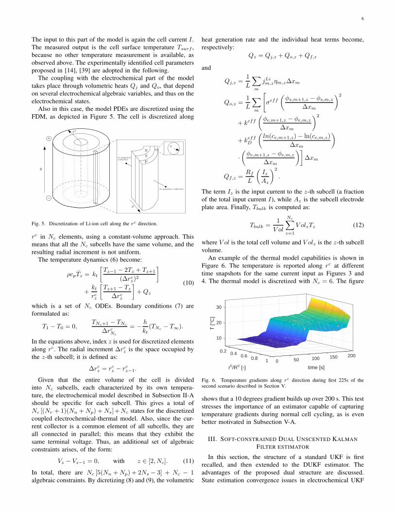
Also in this case, the model PDEs are discretized using the
FDM, as depicted in Figure 5. The cell is discretized along
rc
y
x
+
r
to positive collector
to negative
N
S
P
−
collector
Fig. 5. Discretization of Li-ion cell along the rc direction.
rc in Nc elements, using a constant-volume approach. This
means that all the Nc subcells have the same volume, and the
resulting radial increment is not uniform.
The temperature dynamics (6) become:
ρcpTz = kt
[
Tz−1 − 2Tz + Tz+1
(∆rcz)2
]
+kt
rcz
[
Tz+1 − Tz
∆rcz
]
+Qz
(10)
which is a set of Nc ODEs. Boundary conditions (7) are
formulated as:
T1 − T0 = 0,TNc+1 − TNc
∆rcNc
= −h
kt(TNc
− T∞).
In the equations above, index z is used for discretized elements
along rc. The radial increment ∆rcz is the space occupied by
the z-th subcell; it is defined as:
∆rcz = rcz − rcz−1.
Given that the entire volume of the cell is divided
into Nc subcells, each characterized by its own tempera-
ture, the electrochemical model described in Subsection II-A
should be specific for each subcell. This gives a total of
Nc [(Nr + 1)(Nn +Np) +Ns]+Nc states for the discretized
coupled electrochemical-thermal model. Also, since the cur-
rent collector is a common element of all subcells, they are
all connected in parallel; this means that they exhibit the
same terminal voltage. Thus, an additional set of algebraic
constraints arises, of the form:
Vz − Vz−1 = 0, with z ∈ [2, Nc]. (11)
In total, there are Nc [5(Nn +Np) + 2Ns − 3] + Nc − 1algebraic constraints. By dicretizing (8) and (9), the volumetric
heat generation rate and the individual heat terms become,
respectively:
Qz = Qj,z +Qo,z +Qf,z
and
Qj,z =1
L
∑
m
jLim,zηm,z∆xm
Qo,z =1
L
∑
m
[
σeff
(
φs,m+1,z − φs,m,z
∆xm
)2
+ keff(
φe,m+1,z − φe,m,z
∆xm
)2
+ keffD
(
ln(ce,m+1,z)− ln(ce,m,z)
∆xm
)
·
(
φe,m+1,z − φe,m,z
∆xm
)]
∆xm
Qf,z =Rf
L
(
Iz
Az
)2
.
The term Iz is the input current to the z-th subcell (a fraction
of the total input current I), while Az is the subcell electrode
plate area. Finally, Tbulk is computed as:
Tbulk =1
V ol
Nc∑
z=1
V olzTz (12)
where V ol is the total cell volume and V olz is the z-th subcell
volume.
An example of the thermal model capabilities is shown in
Figure 6. The temperature is reported along rc at different
time snapshots for the same current input as Figures 3 and
4. The thermal model is discretized with Nc = 6. The figure
10
20
0.2
T [°
C]
30
0.4
rc/Rc [-]
2000.6 150
time [s]
0.8 100501 0
Fig. 6. Temperature gradients along rc direction during first 225s of thesecond scenario described in Section V.
shows that a 10 degrees gradient builds up over 200 s. This test
stresses the importance of an estimator capable of capturing
temperature gradients during normal cell cycling, as is even
better motivated in Subsection V-A.
III. SOFT-CONSTRAINED DUAL UNSCENTED KALMAN
FILTER ESTIMATOR
In this section, the structure of a standard UKF is first
recalled, and then extended to the DUKF estimator. The
advantages of the proposed dual structure are discussed.
State estimation convergence issues in electrochemical UKF
7
formulation are studied in simulation and solved by means
of a soft-constraint in Subsection III-A. Finally, a substantial
improvement in computational time is obtained with a parallel
implementation of the DUKF in Subsection III-B.
The UKF is a Sigma-Point Kalman Filter (SPKF) with a
particular choice of weighting coefficients. In [30], details on
UKF formulation and implementation are described, together
with considerations on theoretical aspects. In summary, the
UKF is a model-based estimator for non-linear dynamic sys-
tems, which presents several advantages compared to other
Kalman-based estimators, including EKF:
1) the numeric/analytic computation of Jacobians is not
required;
2) the computational cost is similar to that of EKF; and
3) in turn, accuracy of statistical moments estimation is of
the third order for Gaussian systems [40].
The UKF algorithm is reported in Algorithm 1, for the
case with additive process and measurement noises, indicated
respectively with ξ and υ. A set of sigma-points is determin-
istically sampled starting from the previous-step a-posteriori
state estimate and covariance matrix. In the time-update step,
each of these points is propagated through the system non-
linear state equation; the results are then properly weighted to
generate the current step a-priori state estimate and covariance
matrix. Also, a-priori sigma-points are passed through the
system non-linear output equation, and then properly weighted
to give an estimate of the output and of its covariance matrix.
Furthermore, the state and output cross-covariance matrix
is estimated. Finally, in the measurement-update step, the
Kalman gain is applied to the difference between the actual
and estimated output, in order to compute the current-step
a-posteriori state estimate and covariance matrix. It can be
observed that the time-update step of the algorithm, and in
particular (13) and (14), is naturally amenable to parallel
computing implementation; in fact, each a-priori sigma-point
computation, starting from x+k−1 and P+
xx,k−1, is completely
independent from other sigma-points.
If nx is the dimension of the state vector, the sigma-
points are in the number of 2nx + 1. The covariance matrix
P+xx,0 of the initial state estimate is a tuning parameter, which
rules the initial dispersion of the sigma-points around the
initial state estimate x+0 , that is another tuning parameter.
The covariance matrix Qξξ of the process disturbance and
the covariance matrix Rυυ of the measurement noise are also
important tuning parameters, as well as the other, minor tuning
parameters, such as α, β and κ.
In the present work, the structure of UKF is exploited
twice, so as to obtain the Dual Unscented Kalman Filter
depicted in Figure 7. In this approach, the overall observer
is composed of two parts: the electrochemical UKF and the
thermal UKF. The electrochemical UKF includes only the
P2D model of the cell. It receives as inputs the current and
the estimated bulk temperature, Tbulk, which comes from the
thermal part of the observer; it receives the terminal voltage
as the measured quantity (in the standard approach - see
Subsection III-A for a deeper analysis on this); finally, it
provides estimates of all discretized elements of cs and ce,
gathered in the estimated state vector c, and of the state of
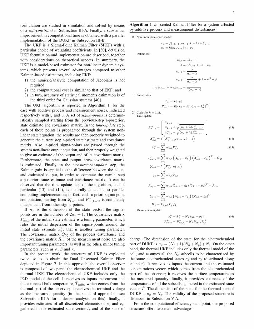
Algorithm 1 Unscented Kalman Filter for a system affected
by additive process and measurement disturbances.
0: Non-linear state-space model:
xk = f(xk−1, uk−1, k − 1) + ξk−1
yk = h(xk, uk, k) + υk
Definitions:
nsp = 2nx + 1
λ = α2(nx + κ) − nx
ws,1 =λ
nx + λ
wc,1 =λ
nx + λ+ 1 − α
2+ β
ws,2:nsp = wc,2:nsp =1
2(nx + λ)
1: Initialization:
x+
0 = E[x0]
P+
xx,0 = E[(x0 − x+
0 )(x0 − x+
0 )T ]
2: Cycle for k = 1, 2, ...Time-update:
X+
k−1=
x+
k−1
x+
k−1+
√
(nx + λ)P+
xx,k−1
x+
k−1−
√
(nx + λ)P+
xx,k−1
(13)
X−
k,i = f(
X+
k−1,i, uk−1, k − 1)
(14)
x−
k =
nsp∑
i=1
ws,iX−
k,i (15)
P−
xx,k =
nsp∑
i=1
wc,i
(
X−
k,i − x−
k
)(
X−
k,i − x−
k
)T+ Qξξ
Yk,i = h(
X−
k,i, uk, k)
yk =
nsp∑
i=1
ws,iYk,i
Pyy,k =
nsp∑
i=1
wc,i (Yk,i − yk) (Yk,i − yk)T + Rυυ
Pxy,k =
nsp∑
i=1
wc,i
(
X−
k,i − x−
k
)
(Yk,i − yk)T
Kk = Pxy,kP−1
yy,k
Measurement-update:
x+
k = x−
k + Kk (yk − yk) (16)
P+
xx,k = P−
xx,k − KkPyy,kKTk
charge. The dimension of the state for the electrochemical
part of DUKF is nx = (Nr+1)(Nn+Np)+Ns. On the other
hand, the thermal UKF includes only the thermal model of the
cell, and assumes all the Nc subcells to be characterized by
the same electrochemical states cs and ce (distributed along
x and r). It receives as inputs the current and the estimated
concentrations vector, which comes from the electrochemical
part of the observer; it receives the surface temperature as
the measured quantity; finally, it provides estimates of the
temperatures of all the subcells, gathered in the estimated state
vector T . The dimension of the state for the thermal part of
DUKF is nx = Nc. The validity of the proposed structure is
discussed in Subsection V-A.
From the computational efficiency standpoint, the proposed
structure offers two main advantages:
8
Elettrochemical UKF
Nn = Ns = Np = 3; Nr = 5
Nc = 1
c−k = fc
(
c+k−1; T+
bulk;k−1; Ik−1
)
Computation
of Tbulk
Thermal UKF
Nn = Ns = Np = 3; Nr = 5
Nc = 6
T−
k = fT
(
T+
k−1; c+k−1
; Ik−1
)
^SoCk
Vk
c+k
I
I
V
Tsurf
T+
k
nt
nt;k
T+
bulk;k−1
1-step delay
1-step delay
Fig. 7. Scheme of the Dual Unscented Kalman Filter estimator. The meaningof the signal nt is explained in Subsection III-A.
1) It automatically solves the problem of the parallel con-
figuration for the subcells. Instead of implementing the
algebraic constraints (11), as is done in the coupled
electrochemical-thermal simulator, the measured quan-
tity V is forced to be the same for all the subcells
through the assumption that all the subcells have the
same electrochemical state c.
2) Compared to a full-order UKF with both electrochemical
and thermal models in a monolithic observer, which
would not be a practical solution due to excessive
computational time, it is much more computationally
manageable. In fact, while still retaining the capability
of estimating both concentrations and temperature gra-
dients, and showing high accuracy, it makes use of the
minimal set of information. From extensive simulation
studies, as those reported in Section V, it is observed
that a bulk estimate of temperature is enough for the
electrochemical part of the observer to accurately es-
timate lithium concentrations in any point of the cell.
Similarly, assuming concentrations are equal among all
discretized subcells is enough for the thermal part of the
observer to correctly estimate the values of temperature
along the cylinder radial direction.
A. Convergence issues with the electrochemical UKF imple-
mentation
It is well known that the lithium concentration is difficultly
estimated from terminal voltage and current measurements.
[41] and [27] discuss the lack of observability for the standard
formulation of the SPM. [42] reaches the same conclusion by
looking at the Jacobian of the Lie derivative of a reduced-
order SPM with addition of electrolyte phase concentrations
dynamics. The analytical analysis of the observability of the
P2D model is made complex by its strong non-linearities and
coupled terms. However, a simple simulation study confirms
the same problem. In this test, the current pulses cycle pre-
sented in Figure 8 is applied to the cell. The standard UKF
0 200 400 600 800 1000
time [s]
-200
0
200
I [A
]
Fig. 8. Convergence issues with the standard application of UKF to SoCestimation: input current profile.
is applied to the discretized P2D model, with Nr = 5 and
Nn = Ns = Np = 3, and with 5% initial SoC error for the
estimator (note that this value is deliberately chosen as small).
This analysis focuses only on the electrochemical part of the
observer, because this is the only one involved in convergence
issues. Figure 9 clearly shows that, while the terminal voltage
estimation error converges to zero, the bulk SoC estimation
error does not tend to 0.
0 200 400 600 800 1000
time [s]
3
3.5
4
4.5V
[V]
simulatedestimated
0 200 400 600 800 1000
time [s]
0
20
40
60
SoC
[%]
simulatedestimated
Fig. 9. Convergence issues with the standard application of UKF to SoCestimation (top: simulated and estimated terminal voltage; bottom: simulatedand estimated SoC).
Figure 10 provide an interpretation of the issue; it plots the
actual and estimated (by using the estimated concentrations)
total number of moles of lithium available in the cell nt. This
0 200 400 600 800 1000
time [s]
0.3
0.4
0.5
nt [m
ol]
simulatedestimated
Fig. 10. Convergence issues with the standard application of UKF to SoCestimation: conservation of total lithium moles in solid phase, under thecurrent profile of Figure 8.
is defined as the sum of the total number of moles of lithium
9
in solid phase ns (which is the integral of cs in the whole
cell volume, i.e. both along r and along x, weighted by the
solid phase volume fraction εs) and the total number of moles
of lithium in electrolyte phase ne (which is the integral of cealong x, weighted by the electrolyte phase volume fraction
εe):
ns =3A
R3s
∫ L
0
∫ Rs
0
εsr2cs drdx
ne = A
∫ L
0
εece dx (17)
nt = ns + ne.
Note that nt is constant for a given cell, and it is directly
computable from known model parameters. The results prove
that the unscented estimation mechanism does not guarantee
the conservation of the total number of moles of available
lithium, or, equivalently, the conservation of total lithium mass.
As a matter of fact, although the single sigma-point transfor-
mation through the model state equation (14) conserves the
total lithium mass, being based on the P2D model formulation,
a few other steps in the UKF algorithm do not provide the
same feature. More in detail, the steps possibly altering the
total lithium mass because of their purely statistical nature
are: 1) sigma-points computation based on previous step a-
posteriori state estimation and covariance matrix (13); 2) a-
priori state estimation via weighted sum of sigma-points (15);
3) a-posteriori state estimation via measurement correction
step (16). Thus, there are 3 specific mechanisms in the UKF
algorithm that are unable to guarantee mass conservation. This
causes the divergence of the estimate.
The structure of the electrochemical UKF is modified to
account for the conservation of lithium, and improve con-
vergence. One could adopt two approaches: a hard-constraint
approach, adding additional algebraic constraints in the sigma-
points computation; or a soft-constraint approach. The latter
idea consists in modifying the input-output structure of the
model by adding a virtual measurement, namely the total
number of moles of available lithium nt (constant signal).
Thus, in Algorithm 1 it holds:
y =
[
V
nt
]
where nt can be computed with (17) starting from the knowl-
edge of the cell physical parameters only. In fact, one can
fix SoC at an arbitrary value, and compute the corresponding
values of cs and ce at steady-state in the whole cell (i.e. in any
point along x and r), by inverting (5). In the electrochemical
UKF tuning, the additive measurement noise variance corre-
sponding to nt is set to a value that is much smaller than
that corresponding to V . Consequently, a soft-constraint is
enforced in the estimator for the conservation of nt, and the
electrochemical model observability is effectively enhanced.
B. Implementation with parallel computing
Each sigma-point propagation through the non-linear state
equation takes place independently from other sigma-points;
this structure is thus suitable for parallel computing implemen-
tation. Most of the time-update step computational cost (i.e.
the one due to the propagation of the sigma points) can be
distributed on multiple cores and optimized, so that the time
required for this step is ultimately significantly reduced.
The following computational cost analysis quantitatively
illustrates this advantage. The dual estimator is run on the
first 100s of the experiment shown in Figure 11. It consists
0 100 200 300 400 500 600
time [s]
0
20
40
60
I [A
]
Fig. 11. Current input profile used to analyze computational cost: pulsessequence at 0-10C.
of a sequence of pulses at 10C followed by rest periods,
both of 10s duration. Simulations were run in MathWorks
MATLAB, with Parallel Computing Toolbox, on a quad-core
machine (2.4GHz) with 12GB RAM and solid-state drive. The
ratio between the simulation time required by the sequential
and parallel implementation, respectively called Tseqsim and
Tparsim, is shown in Figure 12, as a function of Nr, with
Nn = Ns = Np = 3 and Nc = 6. By observing the
2 3 4 5 6 7 8 9 10 11 12 13 14 15
Nr [-]
1
1.5
2
2.5
3
Tsi
mse
q / T
sim
par [-
]
Fig. 12. Ratio between simulation time required by sequential and parallelcomputing implementation of UKF estimator, for different discretization levelsNr .
figure, it is clear that the estimation algorithm computational
burden is reduced by a factor between 1.3 to 2.5 thanks to the
parallel implementation. Note that, on a quad-core machine,
a reduction by exactly a factor 4 is not practically possible,
because of two reasons:
• the observer dual algorithm is not fully parallelizable,
because the electrochemical and thermal parts act on
distinct sets of sigma points;
• some computing overhead is introduced by the Parallel
Computing Toolbox in order to manage the exchange of
information among multiple solvers.
IV. FILTER TUNING ANALYSIS
This section summarizes the results of the DUKF tuning
procedure. The current input profile selected for this purpose is
that of Figure 11. The simulation stops when the output voltage
reaches the lower cutoff value of 2.7V; SoC is roughly 18% at
the end of simulation, because it is not a quasi-static test. The
10
simulator is starting from SoC = 100% and T = 10◦C, while
the estimator is initialized at SoC = 80% and T = 20◦C.
Ambient temperature is kept at Tamb = 10◦C to simulate an
active cooling system acting on the cell. The observer is based
on the following discretization: Nr = 5, Nn = Ns = Np = 3and Nc = 6. Covariance matrices are all chosen as diagonal
matrices, and designed as follows (subscript c stands for the
electrochemical UKF, and T stands for the thermal UKF):
• the covariance matrix P+xx,c,0 of the initial state estimate
has elements on the main diagonal equal to pcs for lines
in the state vector corresponding to cs and pce for lines
corresponding to ce; the covariance matrix P+xx,T,0 has
elements on the main diagonal equal to pT for lines
corresponding to T ;
• the covariance matrix Qξξ,c of the process disturbance
(assumed as an additive Gaussian white noise) has el-
ements on the main diagonal equal to qcs for lines in
the state vector corresponding to cs and qce for lines
corresponding to ce; the covariance matrix Qξξ,T has
elements on the main diagonal equal to qT for lines in
the state vector corresponding to T ;
• the covariance matrix Rυυ,c of the measurement noise
(assumed as an additive Gaussian white noise) has ele-
ments on the main diagonal equal to rV for the line in
the output vector corresponding to V and rnt for the line
corresponding to nt; the covariance matrix Rυυ,T has
elements on the main diagonal equal to rT for the line
in the output vector corresponding to Tsurf .
Due to space limitations, only the sensitivities to a few tuning
parameters are shown here. The sensitivities are presented
separately for the electrochemical UKF and the thermal UKF,
both with an additive noise acting on the measured variables,
in order to understand the estimator robustness with respect to
measurement noises and its actual filtering capability.
A. Tuning of the electrochemical UKF
Given the aforementioned design choices, the study of
the terms in electrochemical covariance matrices follows this
procedure:
• fix pcs = 10−7, pce = 10−10 and pT = 10−1;
• fix qce = 10−12 and qT = 10−6, and study sensitivity to
qcs;
• fix rV = 10−2, rnt = 10−9 (note that, as observed in
Subsection III-A, rnt << rV ) and rT = 10−1.
An additive noise is applied to the simulated voltage signal,
according to the assumptions made above, before feeding it to
UKF for the measurement-update step. The sensitivity analysis
of parameter qcs is performed in Figure 13. εSoC is the bulk-
SoC estimation error, and is defined as the difference between
the simulated and the estimated state of charge. It is used here
as a synthetic figure of the electrochemical UKF accuracy,
while details on local states convergence are presented in
Section V. In this figure, the effect of qcs on estimator
convergence time is clear: the higher is qcs, the lower is the
time needed by UKF to converge to the true value of SoC. This
time may be evaluated, for example, looking at the crossing
of the level εSoC = 5%: this goes from 180s for qcs = 10−8
0 100 200 300 400 500 600
time [s]
0
5
10
15
20
SoC
[%]
qcs
= 10-12
qcs
= 10-11
qcs
= 10-10
qcs
= 10-9
qcs
= 10-8
Fig. 13. Sensitivity study on parameter qcs, under current input profile shownin Figure 11 and additive voltage measurement noise: differently tuned UKFestimators are entering the region at εSoC = 5% at different time instants andshow different noise rejection capability.
to 550s for qcs = 10−12. However, the higher is qcs, the lower
is also the filtering effect of UKF on measurement noise.
In conclusion, a trade-off between convergence time and
estimator rejection/filtering effect in presence of measurement
noise has to be established. After extensive simulation studies,
the selected values for the simulations shown in the following
are qcs = 10−13 and rV = 10−5, that will be exhaustively
validated in Section V.
B. Tuning of the thermal UKF
The tuning study for the thermal covariance matrices has
an analogous procedure:
• fix pcs = 10−7, pce = 10−10 and pT = 10−1;
• fix qcs = 10−11 and qce = 10−12, and study sensitivity
to qT ;
• fix rV = 10−3, rnt = 10−9 and rT = 10+1.
According to the assumptions above, an additive noise is
applied to the simulated surface temperature signal, before
feeding it to UKF for the measurement-update step. The
sensitivity analysis of parameter qT is performed in Figure 14.
εTb is the bulk temperature estimation error, and is defined as
0 100 200 300 400 500 600
time [s]
-10
-8
-6
-4
-2
0
Tb [°
C]
qT
= 10 -6
qT
= 10 -5
qT
= 10 -4
qT
= 10 -3
qT
= 10 -2
qT
= 10 -1
qT
= 10+0
Fig. 14. Sensitivity study on parameter qT , under current input profile shownin Figure 11 and additive surface temperature measurement noise: differentlytuned UKF estimators are entering the region at εTb = −1◦C at differenttime instants and show different noise rejection capability.
11
the difference between the simulated and the estimated bulk
temperature. It is used here as a synthetic figure of the thermal
UKF accuracy, while details on local states convergence are
presented in Section V. The effect of qT on estimator con-
vergence time is evident from the figure: the higher is qT ,
the lower is the time needed by UKF to converge to the true
value of Tbulk. For example, looking at the crossing of the
level εTb = −1◦C, the convergence time goes from 200s for
qT = 10+0 to 500s for qT = 10−6. However, the higher is
qT , the lower is also the noise filtering effect of UKF. In all
considered cases, the estimator is able to fully recover from
wrong initialization. In conclusion, a similar trade-off as for
the electrochemical UKF needs to be settled. After extensive
simulation studies, the selected values used in the following
are qT = 10−6 and rT = 10−1, which will be thoroughly
validated in the next section.
V. VALIDATION
This section validates first the soft-constrained DUKF in two
different scenarios. Then, the advantages of the dual observer
structure are detailed and analyzed in Subsection V-A. All the
simulation results presented hereafter are obtained by relying
on a coupled electrochemical-thermal model, solved via an
ODE solver in MATLAB environment, as explained in [25].
The tests designed for validation purposes are both with
noisy voltage and surface temperature measurements. They are
defined as follows:
1) The current pulses profile at 10C introduced in Subsec-
tion III-B and depicted in Figure 11.
2) A more dynamic test, consisting of a repeating sequence
of current pulses, both positive and negative, with in-
creasing amplitude (as high as 50C or 300A), as shown
in Figure 15; the simulator starts at SoC = 100% and
T = 10◦C (to simulate a cooling system), and the pulses
are designed so that the cell is overall discharging during
the test. As before, the simulation is stopped when V
reaches 2.7V.
0 200 400 600 800 1000 1200
time [s]
-100
0
100
200
300
I [A
]
Fig. 15. Current input profile used to validate the DUKF: sequence of pulsesat increasing amplitude (5C-10C-20C-50C in discharge).
The estimator convergence results for the bulk SoC in the
first test are presented in Figure 16; both SoC and εSoC are
expressed in percentage. The DUKF is initialized at different
initial guesses of SoC and Tbulk, indicated as SoC0,UKF and
T0,UKF, respectively. Also, convergence results for bulk tem-
perature are shown in Figure 17. Temperatures are expressed
in degrees Celsius. It is confirmed that, even in the presence
of noisy measured signals:
0 100 200 300 400 500 600
time [s]
20
40
60
80
100
SoC
[%]
0 100 200 300 400 500 600
time [s]
0
10
20
30
SoC
[%]
SoC0,UKF
= 90% - T0,UKF
= 20°C
SoC0,UKF
= 80% - T0,UKF
= 20°C
SoC0,UKF
= 70% - T0,UKF
= 30°C
SoC0,UKF
= 60% - T0,UKF
= 30°C
SoC0,UKF
= 50% - T0,UKF
= 40°C
Fig. 16. Bulk SoC estimation results for the first scenario, with severalvalues of SoC0,UKF and T0,UKF: for all values of initialization, the estimatorconverges on the true SoC value.
0 100 200 300 400 500 600
time [s]
10
20
30
40
Tbu
lk [°
C]
0 100 200 300 400 500 600
time [s]
-30
-20
-10
0
Tb [°
C] SoC
0,UKF = 90% - T
0,UKF = 20°C
SoC0,UKF
= 80% - T0,UKF
= 20°C
SoC0,UKF
= 70% - T0,UKF
= 30°C
SoC0,UKF
= 60% - T0,UKF
= 30°C
SoC0,UKF
= 50% - T0,UKF
= 40°C
Fig. 17. Bulk temperature estimation results for the first scenario, with severalvalues of SoC0,UKF and T0,UKF: for all values of initialization, the estimatorconverges on the true Tbulk value.
• The estimator is robust enough to recover and finally
converge to the true value of SoC and Tbulk even for a
large initialization error in both the electrochemical and
thermal parts, respectively of up to 50% and up to 30◦C.
• The initial convergence rate is very fast, for all considered
initializations: the SoC error goes below 10% in less than
40s, while the bulk temperature error goes below 5◦C (in
absolute value) in less than 60s.
• After the initial transient (roughly 250s), the SoC error
keeps always under 3% (in absolute value), and reaches
values as low as 1.5% by the end of the test in all
cases apart (SoC0,UKF = 50%, T0,UKF = 40◦C); the bulk
temperature error is always below 0.1◦C (in absolute
value) after the initial transient.
Furthermore, Figure 18 and Figure 19 plot the estimation of
lithium concentration distributions in solid phase at different
time instants. The former figure plots the estimation of surface
stoichiometry for all spherical particles along x, while the
latter figure plots the estimation of stoichiometry along the
12
0 0.2 0.4 0.6 0.8 1
x/L [-]
0.35
0.4
0.45
0.5
0.55
0.6
0.65
0.7
0.75se
[-]
t = 0s
t = 20s
t = 75s
t = 300s
simulatedestimated
Fig. 18. Surface stoichiometry distribution along x direction, at differenttime instants (depicted with different colors) for the first scenario. Verticaldotted lines indicate the separation among domains: negative electrode (left),separator (center) and positive electrode (right).
0 0.2 0.4 0.6 0.8 1
r/Rs [-]
0.4
0.5
0.6
0.7
0.8
0.9
1
s(x=
L,r)
[-]
t = 0s
t = 110s
t = 220s
t = 660s
simulatedestimated
Fig. 19. Stoichiometry distribution along r direction of the spherical particleat x = L, at different time instants (depicted with different colors) for thefirst scenario.
radial direction of a spherical particle close to the positive
current collector. In both cases, the DUKF converges to the
true continuous value of concentrations and accurately esti-
mates the gradients. Note that, in Figure 18, the convergence
of positive electrode states is faster than negative electrode
ones, due to model parameterization and filter tuning. From
Figure 19, it is clear how surface stoichiometry has a faster
convergence over the core one, because the former is the one
more directly affecting the measured voltage. Also, close to the
end of simulation, as can be seen, for example, at t = 660s,
values of surface stoichiometry are reached that are close to
active material saturation/depletion; in these conditions, the
thermodynamic equilibrium potential U exhibits a strong non-
linear dependency on θse. The DUKF observer is effectively
capable of capturing this non-linearity. Finally, Figure 20
shows the temperature distribution in the cylindrical cell at
several time instants. From the figure, it can be seen that the
surface temperature is converging close to the true value in
0.1 0.2 0.3 0.4 0.5 0.6 0.7 0.8 0.9 1
rc/Rc [-]
10
15
20
25
30
35
40
T(r
c ) [°
C]
t = 0s
t = 30st = 80s
t = 660s
simulatedestimated
Fig. 20. Temperature distribution along rc direction of the cylindrical cell,at different time instants (depicted with different colors) for the first scenario.
the first seconds of the test, because it is a measured quantity;
on the contrary, the convergence of the core temperature
requires more time. At the end of the test a gradient of about
7.5◦C is generated between the surface and the core, with the
latter being warmer. This gradient is correctly captured by the
DUKF.
The proposed dual observer is able to estimate both the
bulk SoC and the concentration gradients, as well as the
temperature distribution, also in the second scenario, that en-
compasses a more demanding input. The same representation
used above is followed by Figures 21-25. As before, the
0 200 400 600 800 1000 1200
time [s]
0
50
100
SoC
[%]
0 200 400 600 800 1000 1200
time [s]
0
10
20
30
SoC
[%]
SoC0,UKF
= 90% - T0,UKF
= 20°C
SoC0,UKF
= 80% - T0,UKF
= 20°C
SoC0,UKF
= 70% - T0,UKF
= 30°C
SoC0,UKF
= 60% - T0,UKF
= 30°C
SoC0,UKF
= 50% - T0,UKF
= 40°C
Fig. 21. Bulk SoC estimation results for the second scenario, with severalvalues of SoC0,UKF and T0,UKF: for all values of initialization, the estimatorconverges on the true SoC value.
DUKF estimator is very robust to noisy measurements and
large initial estimation error (of up to 50% and 30◦C). εSoC
converges in all cases to values below 3.5% (in absolute value)
in less than 200s, and below roughly 1.5% by the end of the
test. The same convergence rate is observed in the estimation
of solid particles surface and inner lithium concentrations. εTb
converges in all cases to values below 0.5◦C (in absolute
value) in less than 120s, and similar results are obtained
13
0 200 400 600 800 1000 1200
time [s]
20
40
60
80T
bulk
[°C
]
0 200 400 600 800 1000 1200
time [s]
-30
-20
-10
0
Tb [°
C] SoC
0,UKF = 90% - T
0,UKF = 20°C
SoC0,UKF
= 80% - T0,UKF
= 20°C
SoC0,UKF
= 70% - T0,UKF
= 30°C
SoC0,UKF
= 60% - T0,UKF
= 30°C
SoC0,UKF
= 50% - T0,UKF
= 40°C
Fig. 22. Bulk temperature estimation results for the second scenario, withseveral values of SoC0,UKF and T0,UKF: for all values of initialization, theestimator converges on the true Tbulk value.
0 0.2 0.4 0.6 0.8 1
x/L [-]
0.2
0.3
0.4
0.5
0.6
0.7
0.8
0.9
se [-
]
t = 0s
t = 23s
t = 800s
t = 1100s simulatedestimated
Fig. 23. Surface stoichiometry distribution along x direction, at differenttime instants (depicted with different colors) for the second scenario. Verticaldotted lines indicate the separation among domains: negative electrode (left),separator (center) and positive electrode (right).
for the whole temperature profile along the radius. It is
important to note that, in these conditions with higher currents,
greater internal gradients are triggered, both for concentrations
and temperatures; as such, estimating these gradients is even
more important here. For example, the temperature difference
between the surface and the core of the cell assumes the
substantial value of 35◦C towards the end of the test. Also
in this case, DUKF estimator is capable to overcome the high
non-linearity due to extreme values of surface concentrations
reached in the final part of the test (see for example Figure
24 for t = 1030s).
A. Remark on observer dual structure
This subsection further illustrate the advantages of the dual
structure. The analysis shows that joint temperature and chem-
ical dynamics estimation is required for accurate results; at the
same time, the analysis exemplifies how the DUFK structure
0 0.2 0.4 0.6 0.8 1
r/Rs [-]
0.5
0.6
0.7
0.8
0.9
s(x=
L,r)
[-]
t = 0s
t = 50s
t = 150s
t = 1030s
simulatedestimated
Fig. 24. Stoichiometry distribution along r direction of the spherical particleat x = L, at different time instants (depicted with different colors) for thesecond scenario.
0.1 0.2 0.3 0.4 0.5 0.6 0.7 0.8 0.9 1
rc/Rc [-]
10
20
30
40
50
60
70
80
90
T(r
c ) [°
C]
t = 0s, t = 30s
t = 90s
t = 1150s
simulatedestimated
Fig. 25. Temperature distribution along rc direction of the cylindrical cell, atdifferent time instants (depicted with different colors) for the second scenario.
achieves this result with a limited increase in complexity with
respect to chemical dynamic only estimators.
Consider the electrochemical UKF subject to the input
current of Figure 15, and initialized with 20% initial SoC
error. The simulated temperature profiles from the coupled
electrochemical-thermal model, with Nc = 6, are shown
in Figure 26, for the surface and core subcells. Note that
the simulator is initialized at T = 10◦C. In this study, the
0 200 400 600 800 1000 1200 1400
time [s]
0
50
100
T(r
c ) [°
C] surface
core
Fig. 26. Simulated temperature profiles at surface and core of the cell, underthe same current of Figure 15.
14
electrochemical UKF is run with three different temperature
inputs: (i) a constant temperature equal to Tref , which is
equivalent to fix P2D model parameters to their nominal value,
as if there were no temperature measurement available (see
(5)); (ii) a wrong constant temperature measurement, namely
T = 10◦C, that is the initial cell temperature in the simulated
test, as if there were no thermal dynamics leading to an overall
increase of temperatures; (iii) a bulk temperature measure-
ment, computed from simulated temperature states via (12).
The observer states estimation results can be compared to the
simulated concentrations from the coupled electrochemical-
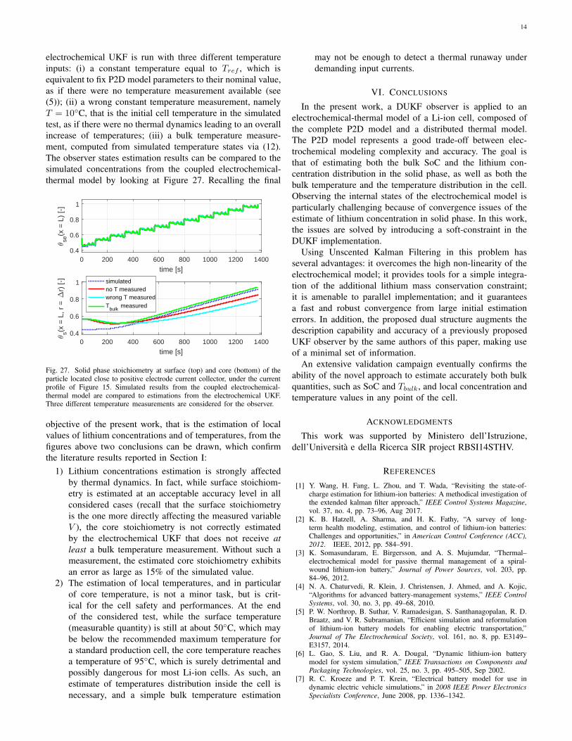
thermal model by looking at Figure 27. Recalling the final
0 200 400 600 800 1000 1200 1400
time [s]
0.4
0.6
0.8
1
se(x
= L
) [-
]
0 200 400 600 800 1000 1200 1400
time [s]
0.4
0.6
0.8
1
s(x =
L, r
=
r) [-
] simulatedno T measuredwrong T measuredT
bulk measured
Fig. 27. Solid phase stoichiometry at surface (top) and core (bottom) of theparticle located close to positive electrode current collector, under the currentprofile of Figure 15. Simulated results from the coupled electrochemical-thermal model are compared to estimations from the electrochemical UKF.Three different temperature measurements are considered for the observer.
objective of the present work, that is the estimation of local
values of lithium concentrations and of temperatures, from the
figures above two conclusions can be drawn, which confirm
the literature results reported in Section I:
1) Lithium concentrations estimation is strongly affected
by thermal dynamics. In fact, while surface stoichiom-
etry is estimated at an acceptable accuracy level in all
considered cases (recall that the surface stoichiometry
is the one more directly affecting the measured variable
V ), the core stoichiometry is not correctly estimated
by the electrochemical UKF that does not receive at
least a bulk temperature measurement. Without such a
measurement, the estimated core stoichiometry exhibits
an error as large as 15% of the simulated value.
2) The estimation of local temperatures, and in particular
of core temperature, is not a minor task, but is crit-
ical for the cell safety and performances. At the end
of the considered test, while the surface temperature
(measurable quantity) is still at about 50◦C, which may
be below the recommended maximum temperature for
a standard production cell, the core temperature reaches
a temperature of 95◦C, which is surely detrimental and
possibly dangerous for most Li-ion cells. As such, an
estimate of temperatures distribution inside the cell is
necessary, and a simple bulk temperature estimation
may not be enough to detect a thermal runaway under
demanding input currents.
VI. CONCLUSIONS
In the present work, a DUKF observer is applied to an
electrochemical-thermal model of a Li-ion cell, composed of
the complete P2D model and a distributed thermal model.
The P2D model represents a good trade-off between elec-
trochemical modeling complexity and accuracy. The goal is
that of estimating both the bulk SoC and the lithium con-
centration distribution in the solid phase, as well as both the
bulk temperature and the temperature distribution in the cell.
Observing the internal states of the electrochemical model is
particularly challenging because of convergence issues of the
estimate of lithium concentration in solid phase. In this work,
the issues are solved by introducing a soft-constraint in the
DUKF implementation.
Using Unscented Kalman Filtering in this problem has
several advantages: it overcomes the high non-linearity of the
electrochemical model; it provides tools for a simple integra-
tion of the additional lithium mass conservation constraint;
it is amenable to parallel implementation; and it guarantees
a fast and robust convergence from large initial estimation
errors. In addition, the proposed dual structure augments the
description capability and accuracy of a previously proposed
UKF observer by the same authors of this paper, making use
of a minimal set of information.
An extensive validation campaign eventually confirms the
ability of the novel approach to estimate accurately both bulk
quantities, such as SoC and Tbulk, and local concentration and
temperature values in any point of the cell.
ACKNOWLEDGMENTS
This work was supported by Ministero dell’Istruzione,
dell’Universita e della Ricerca SIR project RBSI14STHV.
REFERENCES
[1] Y. Wang, H. Fang, L. Zhou, and T. Wada, “Revisiting the state-of-charge estimation for lithium-ion batteries: A methodical investigation ofthe extended kalman filter approach,” IEEE Control Systems Magazine,vol. 37, no. 4, pp. 73–96, Aug 2017.
[2] K. B. Hatzell, A. Sharma, and H. K. Fathy, “A survey of long-term health modeling, estimation, and control of lithium-ion batteries:Challenges and opportunities,” in American Control Conference (ACC),
2012. IEEE, 2012, pp. 584–591.[3] K. Somasundaram, E. Birgersson, and A. S. Mujumdar, “Thermal–
electrochemical model for passive thermal management of a spiral-wound lithium-ion battery,” Journal of Power Sources, vol. 203, pp.84–96, 2012.
[4] N. A. Chaturvedi, R. Klein, J. Christensen, J. Ahmed, and A. Kojic,“Algorithms for advanced battery-management systems,” IEEE Control
Systems, vol. 30, no. 3, pp. 49–68, 2010.[5] P. W. Northrop, B. Suthar, V. Ramadesigan, S. Santhanagopalan, R. D.
Braatz, and V. R. Subramanian, “Efficient simulation and reformulationof lithium-ion battery models for enabling electric transportation,”Journal of The Electrochemical Society, vol. 161, no. 8, pp. E3149–E3157, 2014.
[6] L. Gao, S. Liu, and R. A. Dougal, “Dynamic lithium-ion batterymodel for system simulation,” IEEE Transactions on Components and
Packaging Technologies, vol. 25, no. 3, pp. 495–505, Sep 2002.[7] R. C. Kroeze and P. T. Krein, “Electrical battery model for use in
dynamic electric vehicle simulations,” in 2008 IEEE Power Electronics
Specialists Conference, June 2008, pp. 1336–1342.
15
[8] M. Corno and S. M. Savaresi, “A diffusive electro-equivalent li-ion bat-tery model,” in Circuits and Systems (ISCAS), 2013 IEEE International
Symposium on. IEEE, 2013, pp. 2976–2979.[9] S. Santhanagopalan, Q. Guo, P. Ramadass, and R. E. White, “Review of
models for predicting the cycling performance of lithium ion batteries,”Journal of Power Sources, vol. 156, no. 2, pp. 620–628, 2006.
[10] C. Wang and V. Srinivasan, “Computational battery dynamics(cbd)electrochemical/thermal coupled modeling and multi-scale model-ing,” Journal of power sources, vol. 110, no. 2, pp. 364–376, 2002.
[11] G. G. Botte, V. R. Subramanian, and R. E. White, “Mathematicalmodeling of secondary lithium batteries,” Electrochimica Acta, vol. 45,no. 15, pp. 2595–2609, 2000.
[12] C. Forgez, D. V. Do, G. Friedrich, M. Morcrette, and C. Delacourt,“Thermal modeling of a cylindrical lifepo4/graphite lithium-ion battery,”Journal of Power Sources, vol. 195, no. 9, pp. 2961–2968, 2010.
[13] K. A. Smith, C. D. Rahn, and C. Y. Wang, “Model-based electrochemicalestimation and constraint management for pulse operation of lithium ionbatteries,” IEEE Transactions on Control Systems Technology, vol. 18,no. 3, pp. 654–663, May 2010.
[14] K. Smith and C.-Y. Wang, “Power and thermal characterization of alithium-ion battery pack for hybrid-electric vehicles,” Journal of power
sources, vol. 160, no. 1, pp. 662–673, 2006.[15] Q. Wang, P. Ping, X. Zhao, G. Chu, J. Sun, and C. Chen, “Thermal
runaway caused fire and explosion of lithium ion battery,” Journal of
Power Sources, vol. 208, pp. 210 – 224, 2012.[16] M. Doyle, T. F. Fuller, and J. Newman, “Modeling of galvanostatic
charge and discharge of the lithium/polymer/insertion cell,” Journal of
the Electrochemical Society, vol. 140, no. 6, pp. 1526–1533, 1993.[17] K. Smith and C.-Y. Wang, “Solid-state diffusion limitations on pulse
operation of a lithium ion cell for hybrid electric vehicles,” Journal of
Power Sources, vol. 161, no. 1, pp. 628–639, 2006.[18] K. A. Smith, C. D. Rahn, and C.-Y. Wang, “Control oriented 1d
electrochemical model of lithium ion battery,” Energy Conversion and
management, vol. 48, no. 9, pp. 2565–2578, 2007.[19] A. M. Bizeray, S. Zhao, S. R. Duncan, and D. A. Howey, “Lithium-
ion battery thermal-electrochemical model-based state estimation usingorthogonal collocation and a modified extended kalman filter,” Journal
of Power Sources, vol. 296, pp. 400–412, 2015.[20] J. C. Forman, S. J. Moura, J. L. Stein, and H. K. Fathy, “Genetic param-
eter identification of the doyle-fuller-newman model from experimentalcycling of a lifepo 4 battery,” in American Control Conference (ACC),
2011. IEEE, 2011, pp. 362–369.[21] V. Ramadesigan, V. Boovaragavan, J. C. Pirkle, and V. R. Subrama-
nian, “Efficient reformulation of solid-phase diffusion in physics-basedlithium-ion battery models,” Journal of The Electrochemical Society, vol.157, no. 7, pp. A854–A860, 2010.
[22] J. C. Forman, S. Bashash, J. L. Stein, and H. K. Fathy, “Reduction of anelectrochemistry-based li-ion battery model via quasi-linearization andpade approximation,” Journal of the Electrochemical Society, vol. 158,no. 2, pp. A93–A101, 2011.
[23] P. P. Mishra, M. Garg, S. Mendoza, J. Liu, C. D. Rahn, and H. K.Fathy, “How does model reduction affect lithium-ion battery state ofcharge estimation errors? theory and experiments,” Journal of The
Electrochemical Society, vol. 164, no. 2, pp. A237–A251, 2017.[24] V. R. Subramanian, V. D. Diwakar, and D. Tapriyal, “Efficient macro-
micro scale coupled modeling of batteries,” Journal of The Electrochem-
ical Society, vol. 152, no. 10, pp. A2002–A2008, 2005.[25] L. Onesto, S. Marelli, and M. Corno, “Control-oriented coupled electro-
chemical thermal model for li-ion batteries,” in 2017 IEEE 56th Annual
Conference on Decision and Control (CDC), 2017, pp. 5026–5031.[26] B. Wang, Z. Liu, S. E. Li, S. J. Moura, and H. Peng, “State-of-charge
estimation for lithium-ion batteries based on a nonlinear fractionalmodel,” IEEE Transactions on Control Systems Technology, vol. 25,no. 1, pp. 3–11, 2017.
[27] S. J. Moura, N. A. Chaturvedi, and M. Krstic, “Pde estimation techniquesfor advanced battery management systems, part i: Soc estimation,” inAmerican Control Conference (ACC), 2012. IEEE, 2012, pp. 559–565.
[28] N. Lotfi, R. G. Landers, J. Li, and J. Park, “Reduced-order electrochemi-cal model-based soc observer with output model uncertainty estimation,”IEEE Transactions on Control Systems Technology, vol. 25, pp. 1217–1230, 2017.
[29] M. Corno, N. Bhatt, S. M. Savaresi, and M. Verhaegen, “Electrochemicalmodel-based state of charge estimation for li-ion cells,” IEEE Transac-
tions on Control Systems Technology, vol. 23, no. 1, pp. 117–127, 2015.[30] S. J. Julier, J. K. Uhlmann, and H. F. Durrant-Whyte, “A new approach
for filtering nonlinear systems,” in American Control Conference, Pro-
ceedings of the 1995, vol. 3, Jun 1995, pp. 1628–1632 vol.3.
[31] G. L. Plett, “Sigma-point kalman filtering for battery managementsystems of lipb-based hev battery packs: Part 1: Introduction and stateestimation,” Journal of Power Sources, vol. 161, no. 2, pp. 1356–1368,2006.
[32] S. Santhanagopalan and R. E. White, “State of charge estimation usingan unscented filter for high power lithium ion cells,” International
Journal of Energy Research, vol. 34, no. 2, pp. 152–163, 2010.[33] S. Marelli and M. Corno, “A soft-constrained unscented kalman filter
estimator for li-ion cells electrochemical model,” in 2017 IEEE 56th
Annual Conference on Decision and Control (CDC), 2017, pp. 1535–1540.
[34] G. L. Plett, “Sigma-point kalman filtering for battery managementsystems of lipb-based hev battery packs: Part 2: Simultaneous state andparameter estimation,” Journal of power sources, vol. 161, no. 2, pp.1369–1384, 2006.
[35] J. L. Crassidis and F. L. Markley, “Unscented filtering for spacecraftattitude estimation,” Journal of Guidance Control and Dynamics, vol. 26,no. 4, pp. 536–542, 2003.
[36] S. Al Hallaj, H. Maleki, J.-S. Hong, and J. R. Selman, “Thermalmodeling and design considerations of lithium-ion batteries,” Journal
of Power Sources, vol. 83, no. 1, pp. 1–8, 1999.[37] T. Evans and R. E. White, “A thermal analysis of a spirally wound
battery using a simple mathematical model,” Journal of The Electro-
chemical Society, vol. 136, no. 8, pp. 2145–2152, 1989.[38] S. Anwar, C. Zou, and C. Manzie, “Distributed thermal-electrochemical
modeling of a lithium-ion battery to study the effect of high chargingrates,” IFAC Proceedings Volumes, vol. 47, no. 3, pp. 6258–6263, 2014.
[39] Y. Kim, J. B. Siegel, and A. G. Stefanopoulou, “A computationallyefficient thermal model of cylindrical battery cells for the estimationof radially distributed temperatures,” pp. 698–703, 2013.
[40] E. A. Wan and R. V. D. Merwe, “The unscented kalman filter for non-linear estimation,” in Proceedings of the IEEE 2000 Adaptive Systems
for Signal Processing, Communications, and Control Symposium (Cat.
No.00EX373), 2000, pp. 153–158.[41] D. Di Domenico, A. Stefanopoulou, and G. Fiengo, “Lithium-ion battery
state of charge and critical surface charge estimation using an elec-trochemical model-based extended kalman filter,” Journal of dynamic
systems, measurement, and control, vol. 132, no. 6, p. 061302, 2010.[42] A. Bartlett, J. Marcicki, S. Onori, G. Rizzoni, X. G. Yang, and T. Miller,
“Electrochemical model-based state of charge and capacity estimationfor a composite electrode lithium-ion battery,” IEEE Transactions on
Control Systems Technology, vol. 24, no. 2, pp. 384–399, 2016.