Model Based Parameter Estimation for aMissile

PER HAGG

Masters’ Degree ProjectStockholm, Sweden July 2009

XR-EE-RT 2009:015

Abstract

Traditionally direct integration of the measurements from an IMU (inertial mea-suring unit), measuring the acceleration and inertial angular velocity of the mis-sile, is used to determine a missiles position and state. However, if some priorinformation about the missile dynamics is known, this method should be subop-timal. Combining the knowledge of the missile dynamics with the measurementsshould improve performance.

Of course, the complete missile dynamics are not known. A few model un-certainties are therefore added and these uncertainties are estimated by theestimator. The measurements from the IMU are not perfect and these measure-ment errors are also estimated. This method is called model based parameterestimation.

The problem is non linear and therefore estimators for non linear systemshave been studied. The Extended Kalman filter and the Unscented Kalmanfilter were considered for this problem.

It was shown that using this method the performance of the position estimatecompared to the traditional method, was increased. The performance gain ismainly decided by the size of the model uncertainties compared to the size ofthe measurement errors. All states used in the model was not observable butonly jointly observable meaning that all states did not converge to their truevalue. Instead the error was caught in other states and the position estimatewas still quite good.

Different trajectories for the missile excites different states. The trajectoryboth affects the impact of the IMU-errors and on the observability. The bestperformance was achieved for the sinus trajectory because of its excitation ofthe states. This knowledge might be used to improve the performance for alltrajectories.

An position sensor was also added and the affects were studied. It wasshown that it is possible to increase the estimation performance even if theposition is measured only for a short period of time in the beginning of thetrajectory. The states converged much better using the position sensor thanwithout and this method could be used in the evaluation of fired missiles incontrolled circumstances.

The Extended Kalman filter and the Unscented Kalman filter gave approx-imately the same estimation performance but the Extended Kalman filter wasconsiderably faster and used in most of the analysis of the system. From thisit was concluded that the performance of the position estimate is not estimatordependent but is more about the basic observability of the system.

Contents

1 Introduction 1

1.1 Background . . . . . . . . . . . . . . . . . . . . . . . . . . . . . . 11.2 Problem formulation and goals . . . . . . . . . . . . . . . . . . . 21.3 Method . . . . . . . . . . . . . . . . . . . . . . . . . . . . . . . . 3

2 The missile 4

2.1 Introduction to the missile system . . . . . . . . . . . . . . . . . 42.1.1 Guidance system . . . . . . . . . . . . . . . . . . . . . . . 4

2.2 Deriving a model for the missile . . . . . . . . . . . . . . . . . . . 52.2.1 Coordinate systems . . . . . . . . . . . . . . . . . . . . . 52.2.2 Euler angles . . . . . . . . . . . . . . . . . . . . . . . . . . 62.2.3 Rigid body dynamics . . . . . . . . . . . . . . . . . . . . . 72.2.4 Aerodynamic forces and moments . . . . . . . . . . . . . 82.2.5 Motor model . . . . . . . . . . . . . . . . . . . . . . . . . 102.2.6 Mass changes . . . . . . . . . . . . . . . . . . . . . . . . . 112.2.7 Other forces . . . . . . . . . . . . . . . . . . . . . . . . . . 112.2.8 State space model . . . . . . . . . . . . . . . . . . . . . . 12

2.3 The IMU . . . . . . . . . . . . . . . . . . . . . . . . . . . . . . . 122.3.1 Introduction to the IMU . . . . . . . . . . . . . . . . . . . 122.3.2 IMU model . . . . . . . . . . . . . . . . . . . . . . . . . . 132.3.3 IMU equations . . . . . . . . . . . . . . . . . . . . . . . . 14

2.4 Wind . . . . . . . . . . . . . . . . . . . . . . . . . . . . . . . . . . 14

3 Theory 16

3.1 Estimators . . . . . . . . . . . . . . . . . . . . . . . . . . . . . . . 163.1.1 Kalman filter . . . . . . . . . . . . . . . . . . . . . . . . . 163.1.2 Extended Kalman filter . . . . . . . . . . . . . . . . . . . 173.1.3 Unscented Kalman filter . . . . . . . . . . . . . . . . . . . 18

3.2 Discretization . . . . . . . . . . . . . . . . . . . . . . . . . . . . . 20

4 Implementation 22

4.1 Simulation model . . . . . . . . . . . . . . . . . . . . . . . . . . . 224.1.1 Model uncertainties . . . . . . . . . . . . . . . . . . . . . 244.1.2 IMU errors . . . . . . . . . . . . . . . . . . . . . . . . . . 264.1.3 Flight paths . . . . . . . . . . . . . . . . . . . . . . . . . . 264.1.4 Simulation time . . . . . . . . . . . . . . . . . . . . . . . . 264.1.5 Sampling time . . . . . . . . . . . . . . . . . . . . . . . . 26

4.2 Estimator implementation . . . . . . . . . . . . . . . . . . . . . . 27

i

4.2.1 Extended Kalman filter implementation . . . . . . . . . . 274.2.2 Unscented Kalman filter implementation . . . . . . . . . . 284.2.3 Estimator model implementation . . . . . . . . . . . . . . 284.2.4 Filter tuning . . . . . . . . . . . . . . . . . . . . . . . . . 294.2.5 Implementing the IMU navigation equations . . . . . . . 30

5 Results 31

5.1 Simulations in two dimensions . . . . . . . . . . . . . . . . . . . . 315.1.1 Function test . . . . . . . . . . . . . . . . . . . . . . . . . 315.1.2 Impact of IMU errors on position estimation . . . . . . . 335.1.3 Impact of model errors on position estimation . . . . . . . 355.1.4 Comparison between EKF and UKF . . . . . . . . . . . . 375.1.5 Observability of model errors . . . . . . . . . . . . . . . . 395.1.6 Evaluation of model based parameter estimation . . . . . 475.1.7 Added positioning sensor . . . . . . . . . . . . . . . . . . 54

5.2 Simulations in three dimensions . . . . . . . . . . . . . . . . . . . 57

6 Conclusions and future work 60

6.1 Conclusions . . . . . . . . . . . . . . . . . . . . . . . . . . . . . . 606.2 Future work . . . . . . . . . . . . . . . . . . . . . . . . . . . . . . 61

Bibliography 62

A Parameter values 64

ii

Chapter 1

Introduction

1.1 Background

To be able to guide a missile to a target, at least the position of the missileneeds to be known. The position can be measured using a wide range of differ-ent sensors for example with GPS (Global Positioning System) or with radar.Another way to obtain the position is by calculating the position using mea-surements from an IMU (Inertial Measurement Unit). The IMU measures theinertial acceleration and angular velocity of the missile and from this the stateof the missile is calculated. In this report this method of obtaining the missile’sstate will be considered.

Traditionally the measurements have been directly integrated to obtain theposition. If something about the missile dynamics is known this method byintegrating the measurements should not be optimal. Combining the prior in-formation about the missile dynamics with the measurements should increasethe performance of the position estimate. Usually, good and expensive sensorsare used and not much performance is gained using the prior knowledge of thesystem. Now, however, there is a demand to obtain the position from IMUsin simple and cheap missile systems. In these systems expensive sensors couldnot be used and it should be possible to increase performance by combining themeasurements with prior knowledge about the missile.

In this thesis the performance of a model based parameter estimation methodwill be compared with the classical approach by directly integrating the mea-surements. An estimator will be used to combine the knowledge of the missilewith the measurement. Since the problem is non linear, estimators for nonlinearsystems will be studied.

Another problem that will be considered is what happens if an extra posi-tioning sensor is added. The position is often measured during test firings ofthe missile. Using this information together with the IMU measurments couldgive more information about the internal state of the missile. These extra stateinformation could then be used to evaluate the missiles function and help introubleshooting if something went wrong during the test. It could also be sothat position meassurments are only available in the beginning of the flight, forexample if the position is measured with a short range radar. After this thenavigation is performed only with the IMU. Because of this it has been studied

1

how long the position needs to be measured to improve performance.There are some previous work connected to this problem but these are mainly

for other applications than for a missile. See for example [1], [2] or [3].

1.2 Problem formulation and goals

The main question in this thesis is if, and if this is the case how much, perfor-mance is increased using the model based parameter estimation method. To beable to answer this question a model of the missile needs to be derived. A sim-ulation model is implemented simulating the behaviour of the real missile andgenerating measurements. These measurements are used in order to estimatethe state of the missile. To simulate the missile a realistic simulation model isneeded. This means that all disturbances and model errors needs to be includedin the model. There are however many errors and the number of disturbancesand errors that will be modeled are limited to around ten. The IMU suffers frommeasurements error and these will also be modeled. Only the most importantof these errors will be modeled including the bias, scale factor error and themeasurement noise. The estimator will then from the measurements try to es-timate the model errors and the measurement errors and with this informationtry to estimate the position of the missile better.

The observability of the simulated system will also be studied. The observ-ability will be studied in a practical sense rather than theoretically. From thisit can be concluded which states are observable and how the states depend oneach other. From this analysis it might be possible to reduce the number ofstates.

Different trajectories and their affect on the performance of the estimateswill also be studied. Different trajectories can excite different states in the modeland change the observability. This could mean that certain trajectories to thetarget are better than others when it comes to improving the position estimate.

It could also be interesting to study what happens if a position sensor isadded to the missile. This will of course improve performance considerably.But it could be interesting to see if it is possible to have the position sensor onin a short time in the beginning of the flight and see if the states converge. Afterthe position sensor has been turned off maybe the performance of the positionestimate will be improved.

The case with position measurements during the entire flight time will alsobe studied. This is usually the case during test firings of the missile. Herethe state convergence is studied and not the position estimate. If the statesconverge, this could be used as a tool in the analyze of the test fire.

2

1.3 Method

The first thing to do is to derive a nominal missile model. A model for theIMU is also derived. Then it is decided which disturbances and model errorsthat are going to be included in the model. From this a simulation model isimplemented. The simulation model is used to generate measurements and alsothe real values of the state to be able to compare these to the estimated values.

An estimator model is then derived. This model will differ from the simula-tion model and include more states like model uncertainties and IMU-errors.

The estimators are then implemented. Here the Extended Kalman filter andthe Unscented Kalman filter will be studied. These filters are discrete meaningthat a method for discretization also needs to be implemented.

To begin with the missile will be implemented in two dimensions to simplifythe problems and reduce the size of the model. Most of the questions will beanswered from this system. A three dimensional model will also be used butdue to it’s size and complexity the only thing considered is the performance ofthe model based parameter estimation method.

When these systems are implemented a method is needed to compare thedirect integration method with the model based parameter estimation method.To evaluate the performance for the two methods Monte Carlo simulation isused. From these simulations conclusions are drawn and the questions aboveare answered.

3

Chapter 2

The missile

2.1 Introduction to the missile system

The missile considered here is a generic missile. It is launched from a launchtube and free flies for a short time before its motor starts. The motor is a twostep motor. The first step is the booster step where the missile is acceleratedquickly. The second step is the sustainer step designed to sustain the velocityduring the time of flight.

The missile has control fins acting as aerodynamic control surfaces to beable to control the missile. Changing the angle of these fins generates forcesand moments acting on the missile. An IMU is also mounted in the centerof gravity of the missile to measure the acceleration and the inertial angularvelocity of the missile.

2.1.1 Guidance system

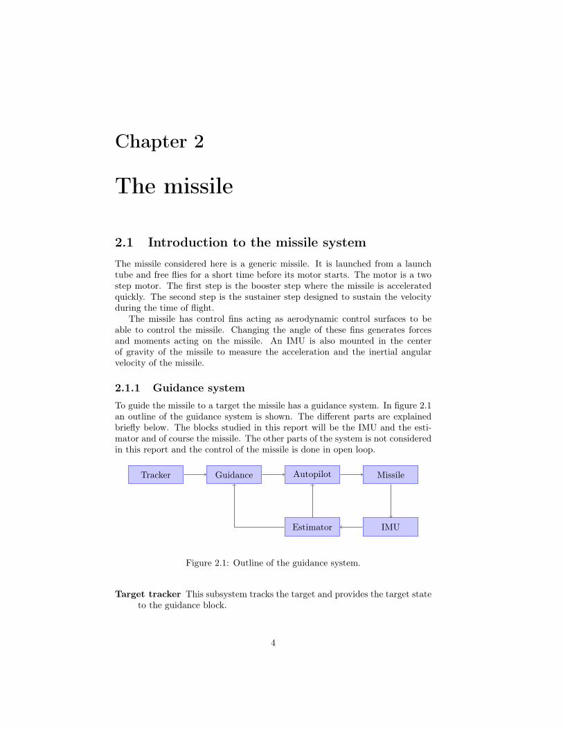
To guide the missile to a target the missile has a guidance system. In figure 2.1an outline of the guidance system is shown. The different parts are explainedbriefly below. The blocks studied in this report will be the IMU and the esti-mator and of course the missile. The other parts of the system is not consideredin this report and the control of the missile is done in open loop.

Tracker Guidance Autopilot Missile

IMUEstimator

Figure 2.1: Outline of the guidance system.

Target tracker This subsystem tracks the target and provides the target stateto the guidance block.

4

Guidance This system uses the information from the tracker to calculate whichtrajectory the missile should follow to hit the target. The trajectory isthen provided to the autopilot.

Autopilot The autopilot calculates what control signals is needed to follow thereference signal from the guidance subsystem.

IMU Measures the acceleration and angular velocity of the missile.

Estimator Estimate the state of the missile from the IMU measurements andtracker.

2.2 Deriving a model for the missile

2.2.1 Coordinate systems

To simplify the calculations, two coordinate systems are introduced. One is sinertial or ground fixed coordinate system and the other one is a missile bodyfixed system. The inertial system is approximated as a ground fixed coordinatesystem. Actually the inertial system is not ground fixed and is moving due tothe earths rotation and other effects. But these effects will not be consideredin this thesis. The body coordinate system on the other hand is moving andfollows the missile. Variables expressed in the two systems are indexed by b andi for the body fixed system and the inertial system respectively. The body fixedcoordinate system is shown in figure 2.2.

Figure 2.2: Definition of the body fixed coordinate system

To express a vector given in the body fixed frame in the inertial frame a trans-formation matrix is needed. Let Tib be a orthonormal transformation matrixsuch that equation 2.2.1 is valid for a arbitrary vector r.

ri = Tibrb (2.2.1)

Then, because of the orthogonality of the transformation matrix, the transformfrom the inertial system to the body fixed system is given by

rb = T−1ib ri = TT

ib ri = Tbiri

5

There are different ways to represent the transformation matrix, here Eulerangles will be used.

2.2.2 Euler angles

Euler angles are used to describe the orientation of the body fixed coordinatesystem relative the inertial coordinate system. The orientation is describes as asequence of three rotations described by the Euler angles. Let the three rotationsbe denoted by φ, θ and ψ. The following rotations are performed:

• ψ around the z axis.

• θ around the new y axis.

• φ around the new x axis.

Simple geometry gives the three rotations in matrix form [4] as

T1 =

cosψ sinψ 0− sinψ cosψ 0

0 0 1

T2 =

cos θ 0 sin θ0 1 0

− sin θ 0 cos θ

T3 =

1 0 00 cosφ − sinφ0 sinφ cosφ

The complete transformation matrix is given by multiplying the three matricesabove

Tib = T1T2T3 =

cos θ cosψ cosψ sin θ sinφ− cosφ sinψ cosφ cosψ sin θ + sinφ sinψcos θ sinψ cosφ cosψ + sin θ sinφ sinψ − cosψ sinφ+ cosφ sin θ sinψ− sin θ cos θ sinφ cos θ cosφ

To be able to use the Euler angles in a dynamic system, the time derivatives ofthe Euler angles need to be derived. If we assume that the angular velocitiesaround the x,y and z axis in the body fixed frame is given respectively by p, qand r then it can be shown that the time derivatives is given [4] by

φ = p +q sinφ tan θ + r cosφ tan θ (2.2.2a)

θ = q cosφ− r sinφ (2.2.2b)

ψ = qsinφ

cos θ+ r

cosφ

cos θ(2.2.2c)

In the equation above the problem with the Euler angles representation is seen.

For cos θ = 0 the system is no longer defined. This occurs when θ =π

2+ πn,

where n is an integer. If this pose a problem then another representations couldbe used, for instance quaternions. This will not be a problem here, since mostof the simulations will be made in a plane with θ = 0. In the three dimensionalcase the flight path will be chosen to avoid this, hence Euler angles will be used.

6

2.2.3 Rigid body dynamics

Before we can set up the equations of motion for the missile a few basic physicalresults are needed [5].

Definition 1 Newton’s second law

F =dp

dt=

d

dt(mv) (2.2.3)

The net force on a particle of constant mass is proportional to the time rate ofchange of its linear momentum.

Definition 2 Euler’s equation

M =dH

dt=

d

dt(Iω) (2.2.4)

The time derivative of angular momentum equals the applied torque.

Theorem 1 The time derivative in a rotating reference frame. Let ωb be thebody’s angular velocity in the body fixed frame. Then the inertial time derivativefor an arbitrary vector rb is given by

(

drbdt

)

i

=

(

drbdt

)

b

+ ωb × rb (2.2.5)

Denote the force and the torque with respect to the center of gravity, appliedto the missile as

F = Fxebx + Fy e

by + Fz e

bz

Mc = M bxc eb

x +M byc eb

y +Mcbz ebz

and the angular velocity as

ω = pebx + qeb

y + rebz

Under the assumption that the moment of inertia tensor,It, and the mass m,for the missile is constant, equation 2.2.3 and equation 2.2.4 combined withequation 2.2.5 gives

F =

(

d (mv)

dt

)

i

= m ( ˙vb + ω × vb) (2.2.6)

Mc = I

(

dω

dt

)

i

= I ( ˙ω + ω × Iω) (2.2.7)

As we will see later the mass is actually not constant. In this case Newtonsequation could not be use. A complete analysis of this problem will give moreterms to the equation. But to simplify the model the mass will be consideredconstant here.

7

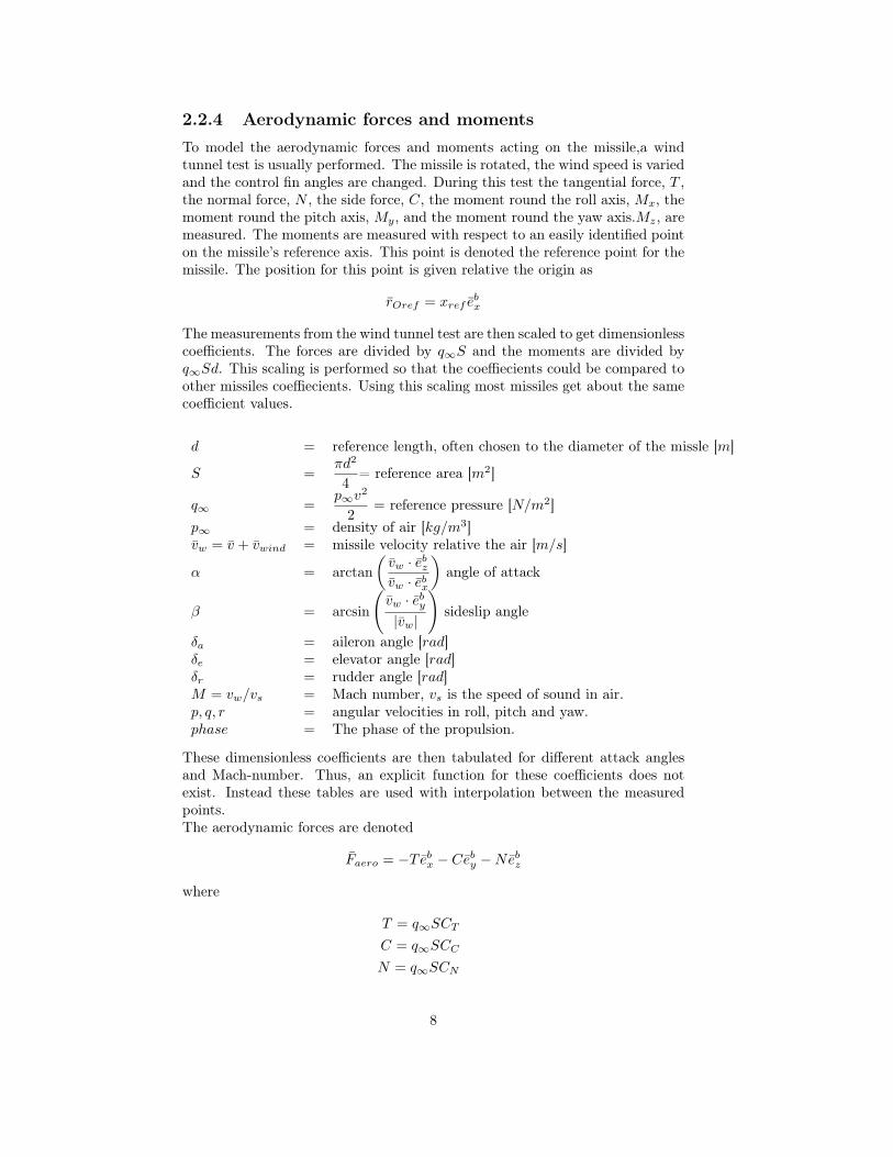
2.2.4 Aerodynamic forces and moments

To model the aerodynamic forces and moments acting on the missile,a windtunnel test is usually performed. The missile is rotated, the wind speed is variedand the control fin angles are changed. During this test the tangential force, T ,the normal force, N , the side force, C, the moment round the roll axis, Mx, themoment round the pitch axis, My, and the moment round the yaw axis.Mz, aremeasured. The moments are measured with respect to an easily identified pointon the missile’s reference axis. This point is denoted the reference point for themissile. The position for this point is given relative the origin as

rOref = xref ebx

The measurements from the wind tunnel test are then scaled to get dimensionlesscoefficients. The forces are divided by q∞S and the moments are divided byq∞Sd. This scaling is performed so that the coeffiecients could be compared toother missiles coeffiecients. Using this scaling most missiles get about the samecoefficient values.

d = reference length, often chosen to the diameter of the missle [m]

S =πd2

4= reference area [m2]

q∞ =p∞v

2

2= reference pressure [N/m2]

p∞ = density of air [kg/m3]vw = v + vwind = missile velocity relative the air [m/s]

α = arctan

(

vw · ebz

vw · ebx

)

angle of attack

β = arcsin

(

vw · eby

|vw|

)

sideslip angle

δa = aileron angle [rad]δe = elevator angle [rad]δr = rudder angle [rad]M = vw/vs = Mach number, vs is the speed of sound in air.p, q, r = angular velocities in roll, pitch and yaw.phase = The phase of the propulsion.

These dimensionless coefficients are then tabulated for different attack anglesand Mach-number. Thus, an explicit function for these coefficients does notexist. Instead these tables are used with interpolation between the measuredpoints.The aerodynamic forces are denoted

Faero = −T ebx − Ceb

y −Nebz

where

T = q∞SCT

C = q∞SCC

N = q∞SCN

8

Figure 2.3: Forces and moments acting on the missile

The moments are written as

Maero = lebx +meb

y + nebz

where

l = q∞SdCl

m = q∞SdCm

n = q∞SdCn

The forces and the moments affecting the missile can be seen in figure 2.3.

The variables CT , CC , CN , Cl, Cm and Cn are the dimensionless coefficientsthat were calculated during the wind tunnel test. These variables is a functionof ϑ = [α, β,M, δa, δe, δr, p, q, r, phase].To simplify calculations and eliminate the need of look up in tables, it is assumedthat the forces and moments are a linear function of the above parameters. Thelinearisation is made around the point

ϑ0 = [α = 0, β = 0,M = 0.4, δa = 0, δe = 0, δr = 0, p = 0, q = 0, r = 0, phase]

To further simplify the model it is assumed that the phase of the motor does notaffect the aerodynamic coefficients. Furthermore it is assumed that the forcecoefficients are independent of the angular velocities and that a control fin anglechange in one channel does not give a direct force or moment contribution in an-other channel. Under these assumptions the aerodynamic can be parameterized

9

as follow

CT

(

ϑ)

= CT

(

ϑ0

)

= CT0

CC

(

ϑ)

= CC

(

ϑ0

)

+

(

∂CC

∂δr

)

(

ϑ0

)

δr +

(

∂CC

∂β

)

(

ϑ0

)

β

= CC0 + CCδrδr + CCββ

CN

(

ϑ)

= CN

(

ϑ0

)

+

(

∂CN

∂δe

)

(

ϑ0

)

δe +

(

∂CN

∂α

)

(

ϑ0

)

α

= CN0 + CNδeδe + CNαα

Cl

(

ϑ)

= Cl

(

ϑ0

)

+

(

∂Cl

∂δa

)

(

ϑ0

)

δa +

(

∂Cl

∂p

)

(

ϑ0

)

p

= Cl0 + Clδaδa + Clpp

Cm

(

ϑ)

= Cm

(

ϑ0

)

+

(

∂Cm

∂δe

)

(

ϑ0

)

δe +

(

∂Cm

∂q

)

(

ϑ0

)

q

+

(

∂Cm

∂α

)

(

ϑ0

)

α

= Cm0 + Cmδeδe + Cmqq + Cmαα

Cn

(

ϑ)

= Cn

(

ϑ0

)

+

(

∂Cn

∂δr

)

(

ϑ0

)

δr +

(

∂Cn

∂r

)

(

ϑ0

)

r

+

(

∂Cn

∂β

)

(

ϑ0

)

β

= Cn0 + Cnδrδr + Cnrr + Cnββ

An good introduction to aerodynamics are given in [6] and [7].

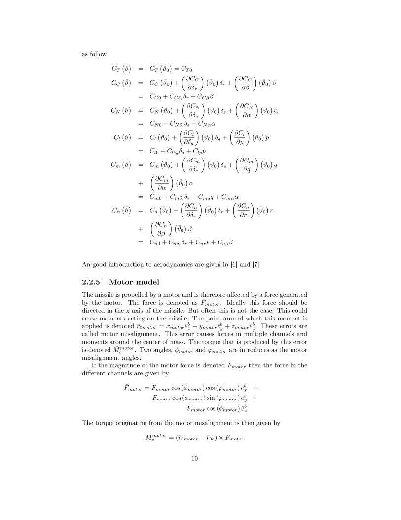
2.2.5 Motor model

The missile is propelled by a motor and is therefore affected by a force generatedby the motor. The force is denoted as Fmotor. Ideally this force should bedirected in the x axis of the missile. But often this is not the case. This couldcause moments acting on the missile. The point around which this moment isapplied is denoted r0motor = xmotor e

bx + ymotor e

by + zmotor e

bz. These errors are

called motor misalignment. This error causes forces in multiple channels andmoments around the center of mass. The torque that is produced by this erroris denoted Mmotor

c . Two angles, φmotor and ϕmotor are introduces as the motormisalignment angles.

If the magnitude of the motor force is denoted Fmotor then the force in thedifferent channels are given by

Fmotor = Fmotor cos (φmotor) cos (ϕmotor) ebx +

Fmotor cos (φmotor) sin (ϕmotor) eby +

Fmotor cos (φmotor) ebz

The torque originating from the motor misalignment is then given by

Mmotorc = (r0motor − r0c) × Fmotor

10

The motor force is generated from a two stage motor. When the missile leavesthe launch tube it free flies for a short period of time before the first motorstarts. The first stage is the booster that accelerates the missile during a shortperiod. The second stage is a sustainer designed to preserve the velocity duringthe time of flight. A motor with the impulse I and the burn time tb generatesthe force during the burn time according to

F =I

tb

The booster’s impulse is denoted with IB and the impulse for the sustainer isdenoted as IS . The burn times for the booster and sustainer is denoted as tBand tS respectively. The time before the booster motor ignites is denoted tign.This gives the magnitude of the force generated by the motor as

Fm(t) =

0 0 ≤ t < tign

IBtB

tign ≤ t ≤ tB

IStS

tB < t ≤ tB + tS

0 t > tB + tS

To make the motor force output more realistic a first order filter is added. Thisfilter is added to avoid steps in the motor force. The filter transfer function isgiven by

Gm(s) =1

1 + τms

where τm is the time constant of the filter.This yields the motor force

Fmotor(t) = Gm(t) ∗ Fm(t) (2.2.11)

2.2.6 Mass changes

When the motor is burning, fuel will be consumed in the missile. This leads toa decrease in mass for the missile. The total mass of the missile is denoted mtot,the booster mass, mb, and the sustainer mass is denoted as ms. The combustionof fuel is assumed to be constant during the different motor phases. This yieldsthe mass as a function of time as

m (t) =

mtot 0 ≤ t < tign

mtot −t

tbmb tign ≤ t ≤ tB

mtot −mb −t− tbts

ms tB < t ≤ tB + tS

mtot −mb −ms t > tB + tS

(2.2.12)

2.2.7 Other forces

Apart from the aerodynamic forces there are other forces acting on the missile.The gravitation will of course affect the missile. However the gravitational forcewill not yield a moment with respect to the center of gravity. The gravitationalforce is given below

Fg = mgeiz

11

2.2.8 State space model

In this sections the equations derived before are summarized into a state spacemodel for the missile. From equation 2.2.6 we get

˙vb =F

m− ω × vb =

1

m

(

Faero + Fmotor + Fg

)

− ω × vb (2.2.13)

The aerodynamic moments are defined with respect to a reference point rOref ,as shown before. This point often differs from the center of mass of the missileand will create a moment around the center of mass. If the center of mass forthe missile is denoted rOc = xce

bx + yce

by + zce

bz, the moment caused by the

aerodynamics forces can be written as

M cF = (rOref − r0c) × Faero (2.2.14)

If the moment of inertia tensor is assumed invertible, equation 2.2.7 gives

˙ω = I−1t Mc − ω × Itω = I−1

t

(

Maero + M cF + Mmotor

)

− ω × Itω (2.2.15)

To calculate the position of the missile the velocities should be integrated. Thevelocities are however given in the body fixed frame and we want the position inthe inertial frame. Therefore the velocities need to be transformed into inertialvelocities before integration. We denote the position of the missile as r =xei

x + yeiy + zei

z. The dynamic equations for the position can then be written as

˙r = Tibvb (2.2.16)

The transformation matrix Tib is given by the Euler angles. Therefore the statespace equations for the Euler angles are needed. These are given by equa-tion 2.2.2

φ = p +q sinφ tan θ + r cosφ tan θ (2.2.17a)

θ = q cosφ− r sinφ (2.2.17b)

ψ = qsinφ

cos θ+ r

cosφ

cos θ(2.2.17c)

To summarize, the state space model is given by the equations above. Thestates are (v, ω, r, φ, θ, ψ).

2.3 The IMU

2.3.1 Introduction to the IMU

A inertial measurement unit (IMU) is a unit that is used to determine the state ofthe missile like velocity and position. The unit consists of three accelerometers,measuring the acceleration of the missile and three gyros, measuring the inertialangular velocities. The acceleration is measured without the gravity

ameas = a− g

where ameas is the measured acceleration, a is the missiles true acceleration andg = (0, 0, g)T

i is the gravity vector. Ideally these should be mounted orthogonal

12

to each other and mounted in the missile such that the measurement axisescoincides with the missile’s axises. This is done to directly get the measurementin the missile body fixed coordinate system. The IMU samples measurementsfrom the accelerometers and gyros and from these measurements the velocity,position and rotation is calculated. But the problem with calculating the missilestate from the IMU measurements is that it accumulates errors. To calculatethe state of the missile from the measurements the detected change in accelera-tion and angular velocities is added to previously calculated states. In the IMUequations section these calculations are described. An error in the measure-ments, irrespective of it’s size, will be accumulated and will eventually causelarge error in the calculated state of the missile. The calculated position willconsequently drift more and more from the real position.

2.3.2 IMU model

In this section a IMU model will be derived. In this model a few of the largestsources of errors are included. The real acceleration and angular velocities forthe missile, expressed in the body fixed frame is denoted

ab = abxe

bx + ab

y eby + ab

z ebz

ω = ωxebx + ωy e

by + ωz e

bz

The first error introduced is the bias error. The bias is added to the measuredsignal. It is varying slowly in time and are therefore usually modeled as aconstant. The bias in the acceleration measurement is denoted abias and thebias in the angular velocities measurements is denoted ωbias. The measuredacceleration and angular velocity is then given by

am = ab − g + abias

ωm = ω + ωbias

Ideally the measurement from the IMU should exactly correspond to thephysical quantity that is measured. But this is not always the case and themeasurement are usually only proportional to the physical quantity. This erroris called a scale factor error and is modeled as

am = Sa

(

ab − g)

ωm = Sωω

where Sa and Sω are the scale factor errors.The final error that is modelled is the measurement noise. Here it will be

modeled as independent white noise.

am = ab − g + wa

ωm = ω + wω

where wa and wω are zero mean white noise with covariance Ra and Rω repet-itively.

The above errors are summed up and the measurements from the IMU are

am = Sa

(

ab − g)

+ abias + wa

ωm = Sωω + ωbias + wω

13

There are other source of errors in the IMU that has not been modeled. Forexample non-linearities in the measurements, that the accelerometers and gyro-scopes are not mounted perfectly or gyro sensitivity to accelerations.

2.3.3 IMU equations

To be able to use the traditional method by integrating the measurements fromthe IMU the IMU navigation equations need to be derived. The accelerationmeasured from the IMU is the missile acceleration without the accelerationfrom gravity. Using the equations 2.2.13 to 2.2.17 with added gravity gives thefollowing state space form.

˙v = am + Tbig − ωm × v

φ = pm + qm sinφ tan θ + rm cosφ tan θ (2.3.1a)

θ = qm cosφ− rm sinφ (2.3.1b)

ψ = qmsinφ

cos θ+ rm

cosφ

cos θ(2.3.1c)

˙r = Tibv (2.3.1d)

where am is the measured acceleration, ωm = (pm, qm, rm)T

is the measured

angular velocity and g = (0, 0, g)T

the gravity vector.

2.4 Wind

During the time of flight the missile is affected by the wind, i.e. the speed of theair surrounding the missile. Here the wind will be modelled as a constant windand as a wind turbulence. The constant wind is given in the inertial frame andthe turbulence in the body fixed frame. Denoting the constant wind vector asvwc and the wind turbulence as vturb yields the total wind velocity as

vbwind = Tbiv

iwc + vb

turb

Wind turbulence is a unpredictable wind that affects the missile. There aremultiple ways to describe the wind turbulence, here a Dryden model will beused. The Dryden model is described as a white noise filtered through a linearfilter. The outputs from the filter are wind speeds given in the body fixed frame.The wind velocities are given by

vturb = Gx (t) ∗ wx (t) ebx +Gy (t) ∗ wy (t) eb

y +Gz (t) ∗ wz (t) ebz (2.4.1)

where wx(t), wy(t) and wz(t) are zero mean independent white noise sources.The transfer functions for the filters in equation 2.4.1 are given in [8] as

Gx (s) =1

1 + sτx

Gy (s) =1 + sτy

√3

(1 + sτy)2

Gz (s) =1 + sτz

√3

(1 + sτz)2

14

The Dryden model given in [8] was originally developed for airplanes flyingat high altitude. Here the wind turbulence will be applied to a missile andtherefore the Dryden model is slightly modified. The missile is, contrary to anairplane, symmetric around its x-axis and therefore the turbulence is modifiedso that it also is symmetric around the x-axis.

The parameters in the filter depends on a few different factors, for example inwhich altitude the missile is flying. Here the turbulence is considered moderateand the altitude to be below 300 meters. Under these conditions the parametersis given by [8] modified to be x-y symmetric as

τi = Li/v

Lx = Ly = Lz =h

(0, 177 + 0, 002743h)1,2

where h is the altitude above ground.

The noise sources standard deviation is given by

σy = σz = 1.6

σx =σz

(0, 177 + 0, 002743h)0,4

The constant wind will be modelled as vwc =(

vwcx, vwcy

, vwcz

)

where the con-stants are generated by a Gaussian distributed random number generated beforethe start of the simulation.

vwcx∼ N

(

0, σ2wcx

)

vwcy∼ N

(

0, σ2wcy

)

vwcz∼ N

(

0, σ2wcz

)

15

Chapter 3

Theory

3.1 Estimators

3.1.1 Kalman filter

The Kalman filter is an optimal recursive filter that estimates the state of adynamic system from noisy measurements. It was introduced in the beginningof 1960s and since then many different variants of the Kalman filter has beendeveloped. If we assume that the measurements are generated from the followinglinear time discrete state space model

x (n+ 1) = F (n)x (n) + w (n) +B(n)u (n) (3.1.1a)

y (n) = H(n)x (n) + e (n) (3.1.1b)

where x (n) is the states of the system and y (n) are the measurements generatedby the system. The stochastic processes w (n) and v (n) are assumed to be zeromean white noise.

E

[(

w (n)e (n)

)

(w (m) , e (m))

]

=

[

Q(n) 00 R

]

δ (n−m)

The processes w (n) and e (n) are usually called process noise and measurementnoise respectively.

The problem that the Kalman filter solves can be expressed asFind the linear estimator x (n|n), of x (n) given the observations y (k), 0 ≤ k ≤n that minimizes the mean square error.

The Kalman filter is given by 3.1.2 and equationequation 3.1.3. A derivation ofthe Kalman filter can be found in [9].

Measurement update:

S(n) = H(n)P (n|n− 1)H(n)T +R (3.1.2a)

K(n) = P (n|n− 1)H(n)TS(n)−1 (3.1.2b)

P (n|n) = P (n|n− 1) −K(n)S(n)K(n)T (3.1.2c)

x(n|n) = x(n|n− 1) +K(n) (y(n) −Hx(n|n− 1)) (3.1.2d)

16

Prediction:

x (n+ 1|n) = F (n)x (n|n) +B(n)u (n) (3.1.3a)

P (n+ 1|n) = F (n)P (n|n)F (n)T +Q(n) (3.1.3b)

where

• x (n|n) is the state estimate.

• P (n) = E[

(x (n) − x (n|n)) (x (n) − x (n|n))T]

is the error covariance

matrix and can be used as a measure of the estimated accuracy of thestate estimate.

The Kalman filter need to be initialized. As the equations are written abovex (0| − 1) and P (0| − 1) are needed. A more thorough investigation of theKalman filter could be found in for example [10] or [11].

3.1.2 Extended Kalman filter

For the Kalman filter to be optimal the state space model needs to have theform as given in equation 3.1.1 . If the state space model is non-linear theKalman filter can not be used directly. A first step to create a Kalman filter fora non-linear system is to linearize the state space equations around a nominaltrajectory. But this only gives sufficient performance if the real trajectory isclose enough to the nominal trajectory. In the Extended Kalman filter (EKF)this problem is solved by linearize around the previous state estimate. Moreabout the Extended Kalman filter could be found in [11]. We assume thatthe measurements has been generated from the following non-linear state spacemodel

x (n+ 1) = f (x (n) , u (n)) + w (n) (3.1.4a)

y (n) = h (x (n)) + e (n)

The Kalman filter from the previous section is used but with the difference thatthe matrices F and H is approximated by the Jacobians

H (n) =∂h

∂x

∣

∣

∣

∣

x(n|n−1)

(3.1.5a)

F (n) =∂f

∂x

∣

∣

∣

∣

x(n−1|n−1),u(n)

The complete Extended Kalman filter is then given by the followingMeasurement update:

H (n) =∂h

∂x

∣

∣

∣

∣

x(n|n−1)

S(n) = H(n)P (n|n− 1)H(n)T +R

K (n) = P (n|n− 1)H(n)TS(n)−1

x (n|n) = x (n|n− 1) +K (n) (y (n) − h (x (n|n− 1)))

P (n|n) = P (n|n− 1) −K(n)S(n)K(n)T

17

Prediction:

F (n) =∂f

∂x

∣

∣

∣

∣

x(n|n),u(n)

x (n+ 1|n) = f (x (n|n) , u(n))

P (n+ 1|n) = F (n)P (n|n)F (n)T +Q(n)

The Extended Kalman filter is not optimal as the Kalman filter. Problems canoccur if the state estimate differs to much from the true states. This could causethe linearization to be a bad approximation and the estimates could diverge.

3.1.3 Unscented Kalman filter

The Unscented Kalman filter is a relatively new filter presented by Julier andUhlmann in 1997. [12] The main idea behind the Unscented Kalman filter(UKF)is that it is easier to approximate a Gaussian distribution than to approximatea non-linear function. A deterministic sampling technique is used to generatea set of sample points, often called sigma points. These sigma points are thenpropagated through the non-linear system and the result are used to approxi-mate how the mean and covariance are affected by the non-linearities.We assume that the non-linear state space system that generates the measure-ments is on the following form

x (n+ 1) = f (x (n) , u (n) , w (n))

y (n) = h (x (n) , e (n))

where w (n) and e (n) are zero mean white noises with the covariance matricesQ and R respectively.The vector xa (n) is introduced as the augmented state vector given by

xa (n) =[

x (n)Tw (n)

Te (n)

T]T

The state estimate vector x (n) is also introduced.

The algorithm for the Unscented Kalman filter is as follow

Start by choosing sigma points, χin. Usually, N = 2nx + 1 sigma points are

chosen, where nx is the dimension of xa. The sigma points are generated as

χ0n−1 = x (n− 1)

χin−1 = x (n− 1) +

(√

(nx + λ)P an−1

)

i, i = 1 . . . nx

χin−1 = x (n− 1) −

(√

(nx + λ)P an−1

)

nx−i, i = nx + 1 . . . 2nx

where(

√

(nx + λ)Pn−1

)

iis the i:th column of the matrix square root. B is

matrix square root of A if A = BBT .λ is defined as

λ = α2 (nx + κ) − nx

18

The parameters α, β and κ are design parameters and can be chosen arbitrary.According to [13] α = 10−3, β = 2 and κ = 0 are recommended and will be used.

The sigma points are now propagated through the non-linear system dynamics

χin = f

(

χin−1, u(n− 1)

)

, i = 0 . . . 2nx

The a priori state estimate is then calculated as

x− (n) =

2nx∑

i=0

Wmi χi

n

and the a priori error covariance matrix as

P−n =

2nx∑

i=0

W ci

[

χin − x− (n)

] [

χin − x− (n)

]T

The weights Wmi and W c

i is defined as

Wmi =

λ

nx + λi = 0

λ

2 (nx + λ)i = 1 . . . 2nx

W ci =

λ

nx + λ+(

1 − α2 + β)

i = 0

λ

2 (nx + λ)i = 1 . . . 2nx

The predicted measurement are calculated based on the sigma points

Υin = h

(

χin

)

, i = 0 . . . 2nx

yielding

y− (n) =

2nx∑

i=0

Wmi Υi

n

The Kalman gain is then calculated as

Kn = PxnynP−1

ynyn

where

Pynyn=

2nx∑

i=0

W ci

[

Υin − y− (n)

] [

Υin − y− (n)

]T

Pxnyn=

2nx∑

i=0

W ci

[

χin − x− (n)

] [

Υin − y− (n)

]T

19

The a posteriori state estimate is then calculated as

x (n) = x− (n) +Kn

(

y (n) − y− (n))

where y (n) the measured signal.

Finally the a posteriori estimate of the error covariance matrix is calculated

Pn = P−n −KnPynyn

KTn

Set n = n+ 1 and restart the algorithm.

The UKF must be initiated for n = 0 with the following values

x0 = E [x0]

P0 = E[

[x0 − E[x0]] [x0 − E[x0]]T]

xa0 = E [xa] =

[

xT0 0 0

]T

P a0 = E

[

[xa0 −E[xa

0 ]] [xa0 − E[xa

0 ]]T]

=

P0 0 00 Q 00 0 R

3.2 Discretization

The Kalman filters are time discrete filters. If a time continuous model hasbeen derived for a system, it need to be discretized in order to be used by theKalman filter. In this section, discretization of a time continuous state spacemodel is discussed.

Assume the following continuous time linear state space model

x (t) = Fx (t) +Bu (t) + w (t) (3.2.1)

y (t) = Hx (t) +Du (t) + e (t) (3.2.2)

where w(t) and e(t) are independent white noise with the following distribution

w(t) ∼ N (0, Q)

e(t) ∼ N (0, R)

20

Assuming that the input, u(t) is constant during one sample period, Ts, themodel in 3.2.1 be discretized [14] to

x (n+ 1) = Fdx (n) +Bdu (n) + w (n) (3.2.3)

y (n) = Hdx (n) +Ddu (n) + e (n)

w(n) and e(n) are time discrete white noise processes, distributed as

w(n) ∼ N (0, Qd)

e(n) ∼ N (0, Rd)

where

Fd = eFTs (3.2.4a)

Bd =

∫ Ts

τ=0

eFτBdτ (3.2.4b)

Hd = H (3.2.4c)

Dd = D (3.2.4d)

Qd =

∫ Ts

τ=0

eFτQeF T τdτ (3.2.4e)

Rd = R (3.2.4f)

The integrals involving the matrix exponential in equation 3.2.4 can be hardto calculate. The integral calculations could however be transformed to ma-trix exponential calculations, which is easier to solve numerically. In [15] it isdescribed how this transformation is made and how to calculate the matrix ex-ponentials numerically.For example, the process noise covariance could be calculated in the followingway.

Start by calculating

G = exp

([

−F Q0 FT

])

=

[

F2 G2

0 F3

]

It can then be shown that the discritizized covariance matrix is given by

Qd = FT3 G2

21

Chapter 4

Implementation

4.1 Simulation model

A simulation model of the missile will be implemented in Simulink. The simu-lation model will be used to generate IMU measurements. These measurementsare then filtered through the Kalman filters to estimate the state of the system.The real states will also be saved from from the simulation model to be ableto evaluate the performance of the estimators. The state space system given insection 2.2.8 is used. The complete simulation model is summarized below. Allparameter values can be found in appendix A.

˙vb =1

m

(

Faero + Fmotor + Fg

)

− ω × vb

˙ω = I−1t

(

Maero + M cF + Mmotor

)

− ω × Itω

φ = p+ q sinφ tan θ + r cosφ tan θ

θ = q cosφ− r sinφ

ψ = qsinφ

cos θ+ r

cosφ

cos θ˙r = Tibvb

22

where

Fmotor = Fmotor cos (φmotor) cos (ϕmotor) ebx +

Fmotor cos (φmotor) sin (ϕmotor) eby +

Fmotor cos (φmotor) ebz

Mmotorc = (r0motor − r0c) × Fmotor

Fg = mgeiz

Faero = −q∞S(

CT ebx + CC e

by + CN e

bz

)

Maero = q∞Sd(

Clebx + Cme

by + Cne

bz

)

CT = CT0

CC = CC0 + CCδrδr + CCββ

CN = CN0 + CNδeδe + CNαα

Cl = Cl0 + Clδaδa + Clpp

Cm = Cm0 + Cmδeδe + Cmqq + Cmαα

Cn = Cn0 + Cnδrδr + Cnrr + Cnββ

α = arctan

(

vw · ebz

vw · ebx

)

β = arcsin

(

vw · eby

|vw|

)

vw = vb + vwind = vb + Tbiviwc + vb

turb

The motor force, Fmotor are given from equation 2.2.11 and the mass, m, byequation 2.2.12.

The wind turbulence model from section 2.4 will also be implemented.

vbturb = Gx (t) ∗ wx (t) eb

x +Gy (t) ∗ wy (t) eby +Gz (t) ∗ wz (t) eb

z

where wx(t), wy(t) and wz(t) are zero mean independent white noise sources.

Gx (s) =1

1 + sτx

Gy (s) =1 + sτy

√3

(1 + sτy)2

Gz (s) =1 + sτz

√3

(1 + sτz)2

The output from the simulation model will be the measurement from the IMU.The IMU measures the acceleration and angular velocity in the body fixed frame.The sampling time for the IMU will be set as Ts = 0.01. The acceleration is

not a state itself but it is given by ab =1

m

(

Faero + Fmotor + Fgravity

)

. This

combined with the IMU measurement equations from section 2.3.2 gives thefollowing measurement from the simulation model

am = (1 + Sa)1

m

(

Faero + Fmotor

)

+ abias + wa

ωm = (1 + Sω) ω + ωbias + wω

23

The control fin angles δa, δe and δr are regarded as the inputs to the system.

4.1.1 Model uncertainties

The simulation model given above is the nominal missile model. But in thismodel we have a few model parameter uncertainties and errors. In this sectionthese uncertainties will be modeled.

Motor force error

The force generated by the motor is not exactly known. This error is modeledas a scale factor error

F realm = SFm

Fm

where SFmis the scale factor error modeled as

SFm∼ N

(

1, σ2SFm

)

Motor misalignment error

The motor force is not perfectly directed along the missiles x-axis. This causesforces in the other channels as described in section 2.2.5. The motor misalign-ment error is given by the angles φmotor and ϕmotor. These are modeled as

φmotor ∼ N(

0, σ2φmotor

)

ϕmotor ∼ N(

0, σ2ϕmotor

)

Control fin angle errors

The control fins of the missile could cause other forces and moments than thenominal model predicted. This is modeled as a scale factor error on the rudderaerodynamic coefficients.

Creallδa

= SlδaCnominal

lδa

CrealCδr

= SCδrCnominal

Cδr

Crealnδr

= SnδrCnominal

nδr

CrealNδe

= SNδeCnominal

Nδe

Crealmδe

= SmδeCnominal

mδe

The scale factor errors SCδrand Snδr

are modeled as

Slδr∼ N

(

1, σ2Slδa

)

SCδr∼ N

(

1, σ2SCδr

)

Snδr∼ N

(

1, σ2Snδr

)

SNδr∼ N

(

1, σ2SNδe

)

Smδr∼ N

(

1, σ2Smδe

)

24

Errors in other aerodynamic coefficients

Uncertainties in the other aerodynamic coefficients will also be modeled. Westart by modelling a uncertainty in the drag coefficient CT0. Uncertainties inthe force and moments coefficients due to the angle of attack and sideslip anglewill also be modeled. These will also be modeled as a scale factor error.

CrealT0 = ST0C

nominalT0

Crealnβ = SnβC

nominalnβ

CrealCβ = SCβC

nominalCβ

Crealmα = SmαC

nominalmα

CrealNα = SNαC

nominalNα

where the scalefactor errors is modeled as

ST0 ∼ N(

1, σ2ST0

)

Snβ ∼ N(

1, σ2Snβ

)

SCβ ∼ N(

1, σ2SCβ

)

Smα ∼ N(

1, σ2Smα

)

SNα ∼ N(

1, σ2SNα

)

Air density uncertainty

Uncertainty in the air density will be modeled as

preal∞ = Sp∞

pnominal∞

where Sp∞is the scale factor error modeled as

Sp∞∼ N

(

1, σ2Sp∞

)

Mass uncertainty

Finally the uncertainty in the missile mass will be modeled. In reality threemass errors needs to be modeled, one for the total missile mass, one for thebooster motor and one for the sustainer motor mass. But to reduce the modelsize only one scale factor error is implemented to represent all these errors.

mreal(t) = Smm

nominal(t)

where Sm is the scale factor error modeled as

Sm ∼ N(

1, σ2Sm

)

25

4.1.2 IMU errors

The IMU errors are assumed to be constant during the simulation time and willbe generated before the simulation starts. The following models will be used togenerate the IMU errors

abiasx∼ N(0, σ2

ax)

abiasy∼ N(0, σ2

ay)

abiasz∼ N(0, σ2

az)

ωbiasp∼ N(0, σ2

ωp)

ωbiasq∼ N(0, σ2

ωq)

ωbiasr∼ N(0, σ2

ωr)

Sax∼ N(0, σ2

Sx)

Say∼ N(0, σ2

Sy)

Saz∼ N(0, σ2

Sz)

Sωp∼ N(0, σ2

Sp)

Sωq∼ N(0, σ2

Sq)

Sωr∼ N(0, σ2

Sr)

4.1.3 Flight paths

The affect of the trajectory on the estimation performance will be considered.To simplify the analysis only three basic trajectories will be studied. Thesethree trajectories are

• A straight path, with δr = 0.025.

• A constant turn, with δr = 0.025.

• A trajectory were the control fin angle is a low frequency sinus wave givenby δr = 0.025 sin (2.3t)

4.1.4 Simulation time

The simulation time will be chosen as 20 s. This time is chosen to catch alleffects and the transients caused by the motor. 20 s is also an reasonable timeconsidered the range of the missile. .

4.1.5 Sampling time

The sample time is chosen to Ts = 0.01 s. The value is chosen from previousexperience of reasonable sampling times in an missile application and is also angood compromise between performance and execution time for the filters.

26

4.2 Estimator implementation

4.2.1 Extended Kalman filter implementation

We start with the implementation of the Extended Kalman filter. The ExtendedKalman filter given in section 3.1.2 requires a system in time discrete form. Butthe missile system is given as a time continuous state space model. The missilesystem could be discretized but since it is a non-linear system it could be verydifficult. Instead a variant of the Extended Kalman filter will be used withcontinuous system dynamics but time discrete measurement equations.First we study the time update of the filter, in the EKF from the theory chapter.The prediction step

x (n+ 1|n) = fd (x (n|n) , u(n))

is replaced by solving the following differential equation.

x (n+ 1|n) = x((n+ 1)Ts)

where x((n+ 1)Ts) is the solution to the differential equation

x (t) = f (x (t) , u (t))

withx(nTs) = x (n|n)

where the function f is the time continuous function. This differential equationwill be solved numerically in each time update step. In this implementationRunge-Kutta 4 is used as the numerical solver. More about Runge-Kutta 4 canbe found in [16].

To calculate the posterior error covariance matrix the discrete Jacobian F (n) isneeded. The problem is that we have a time continuous function that is diffi-cult to discretize. To get around this problem, first the Jacobian for the timecontinuous system equation is calculated. This Jacobian is then discretized andused in the Kalman filter. Hence

Jf(t) =∂f

∂x

∣

∣

∣

∣

x(n|n),u(n)

The Jacobian for the time continuous system is then discretizied with equa-tion 3.2.4.

F (n) = eJf(t)Ts

The only thing left in the prediction step is to calculate Q (n) from the contin-uous process noise covariance matrix. For this we use the result from section3.2. Now the posterior error covariance matrix is calculate as

P (n+ 1|n) = F (n)P (n|n)F (n)T +Q(n)

No changes are done to the measurement update step in the Extended Kalmanfilter.

27

4.2.2 Unscented Kalman filter implementation

The Unscented Kalman filter is also a time discrete filter. The same problemoccur with the time continuous state space description of the missile as withthe Extended Kalman filter. But the only thing needed changing from theUnscented Kalman filter in section 3.1.3 is the prediction of the sigma points.

χin = fd

(

χin−1, u(n− 1)

)

, i = 0 . . . 2nx

Since the function f() in this case is a time discrete function this step need tobe replaced. This is done as in the EKF implementation in the previous section.

χin = x(nTs)

where x(nTs) is the solution to the following differential equation

x (t) = f (x (t) , u (t))

withx((n− 1)Ts) = χi

n−1

where the function f is the time continuous missile system dynamic function.This is repeated for i = 0 . . . 2nx.Again these differential equations are solved with the Runge-Kutta 4 method.

4.2.3 Estimator model implementation

It has been shown that a time continuous state space model can be used for theKalman filters. This means that the model from the simulation section can beused. Of course only the nominal model is known and not the true values ofall the parameters. But these parameters will be estimated by the estimator.This leads to the extended model with included the scale factor errors and themotor misalignment angles as states. The wind turbulence is excluded from themodel but the constant wind will be estimated. To improve the measurementfrom the IMU the measurement error parameters will also be estimated andincluded as states in the model. The covariances of all theses error parametersare assumed known. This lead to the following extension of the model given inthe simulation section.

28

SFm= 0

φmotor = 0

ϕmotor = 0

Slδr= 0

SCδr= 0

Snδr= 0

SNδr= 0

Smδr= 0

ST0 = 0

Snβ = 0

SCβ = 0

Smα = 0

SNα = 0

Sp∞= 0

Sm = 0

vwcx= 0

vwcy= 0

vwcz= 0

abiasx= 0

abiasy= 0

abiasz= 0

ωbiasp= 0

ωbiasq= 0

ωbiasr= 0

Sax= 0

Say= 0

Saz= 0

Sωp= 0

Sωq= 0

Sωr= 0

4.2.4 Filter tuning

Both the Extended Kalman filter and the Unscented Kalman filter has param-eters that can be changed to tune the filter performance. In common for thetwo filters is the possibility to tune the values for the process noise covariancematrix and the measurement noise covariance matrix to improve performance.The process noise covariance is often tuned to include possible model errors. For

29

the Unscented Kalman filter the parameters α, β and κ could also be tuned.But in this case the system is large and complex and it is hard and time con-suming to try to tune all parameters. Instead the covariance matrices will bechosen such that they correspond to their physical value in the system. Themeasurement covariance matrix will thus be chosen as the variances of the mea-surement noises as its diagonal elements. If we for a moment disregard the windturbulence, no process noises affects the system and the process noise covari-ance matrix is chosen to the zero matrix. The wind turbulence must howeverbe added. By looking at the simulation model above it is seen that the windturbulence enters the system at the same places as the constant wind. Thismeans that the wind turbulence could be seen as noise on the constant windstates and thus we add some value in the diagonal element in the process noisecovariance matrix, representation the constant wind states. Hopefully this un-certainty also will spread itself through the system to handle the model errorsoriginating from, for example, the linearization of the EKF and the fact that wesamples the system. This method is tested and the process noise covariance forthe constant wind is tuned. From these test we can conclude that the methodfunctions and the value of the process noise covariance for the constant wind ischosen to 25.

4.2.5 Implementing the IMU navigation equations

The state estimation will be implemented using the IMU equations given insection 2.3.3. Again these equations is given in continuous time but the systemis sampled and time discrete. This is done by solving the differential equationgiven by equation 2.3.1. This differential equation is solved with Runge Kutta 4.The estimate of the the states at discrete time n is given by x (n) where

x (n) = x(nTs)

where x(nTs) is the solution to the differential equation

x (t) = f (x (t) , u (t))

withx((n− 1)Ts) = x (n− 1|n− 1)

where the function f is the time continuous function given in equation 2.3.3.

30

Chapter 5

Results

5.1 Simulations in two dimensions

Most of the analysis will be made in two dimensions to reduce the number ofstates and simplify the problem. The parameter values used in this case can befound in appendix A.

5.1.1 Function test

The first thing to do is to verify the function of the state estimation with theExtended Kalman filter and the traditional navigation equations. No IMU mea-surement errors or model uncertainties are included in this verification. Ideally,with no measurement errors or model uncertainties, the estimation should con-tain no errors. But a sampled system is used which lead to errors in the esti-mation. In the Extended Kalman filter the linearisation and discretization alsocould lead to errors. The results from this verification gives, in some sense, thebest possible performance the two different methods. The simulation is per-formed for the three basic trajectories. In figure 5.1 the estimation errors areshown for the straight trajectory. The estimation errors are only shown for thevelocity in x-direction and the x-position since all other errors are zero for thestraight trajectory.

31

0 1 2 3 4 5 6 7 8 9 10 11 12 13 14 15 16 17 18 19 20−0.2

0

0.2

0.4

0.6

0.8

1

1.2

1.4Estimation error vx

Time [s]

Vel

oci

tyer

ror

[m/s]

0 1 2 3 4 5 6 7 8 9 10 11 12 13 14 15 16 17 18 19 200

0.2

0.4

0.6

0.8

1

1.2Estimation error x

Time [s]

Dis

tance

erro

r[m

]

Figure 5.1: Estimation errors for: EKF - solid, IMU equations - dashed, for thestraight trajectory. Sampling time Ts = 0.01 s.

In the figure it can be seen that the estimation error for the Extended Kalmanfilter is small compared to the estimation error with the IMU equations. At0.3 s, when the booster motor ignites the estimation error for the traditionalnavigation method increases. When the velocity is calculated with the IMUequations the accelerations are assumed constant during the sampling periodas show in section 2.3.3. If the true acceleration changes between two samplesthe calculated velocity will differs from the true velocity. The booster engineaccelerates the missile rapidly. Hence we get a large change in the accelerationbetween two samples which gives an estimation error. The same behavior canbe seen when the booster motor and the sustainer motor extincts at 0.8 s and12.8 s respectively. The EKF on the other hand do not get these errors. Thisis because the EKF uses the model of the missile to estimate the accelerationbetween the samples as well.

To verify that the estimation errors are due to the sampling a new simulationis performed with a shorter sampling time. The sampling time is set to Ts =0.001 s which is ten times lower than the previous sampling time. This shoulddecrease the estimation error since the acceleration change between the samples

32

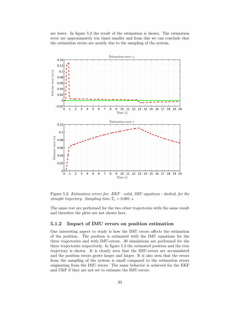
are lower. In figure 5.2 the result of the estimation is shown. The estimationerror are approximately ten times smaller and from this we can conclude thatthe estimation errors are mostly due to the sampling of the system.

0 1 2 3 4 5 6 7 8 9 10 11 12 13 14 15 16 17 18 19 20−0.02

0

0.02

0.04

0.06

0.08

0.1

0.12

0.14Estimation error vx

Time [s]

Vel

oci

tyer

ror

[m/s]

0 1 2 3 4 5 6 7 8 9 10 11 12 13 14 15 16 17 18 19 200

0.02

0.04

0.06

0.08

0.1

0.12Estimation error x

Time [s]

Dis

tance

erro

r[m

]

Figure 5.2: Estimation errors for: EKF - solid, IMU equations - dashed, for thestraight trajectory. Sampling time Ts = 0.001 s.

The same test are performed for the two other trajectories with the same resultand therefore the plots are not shown here.

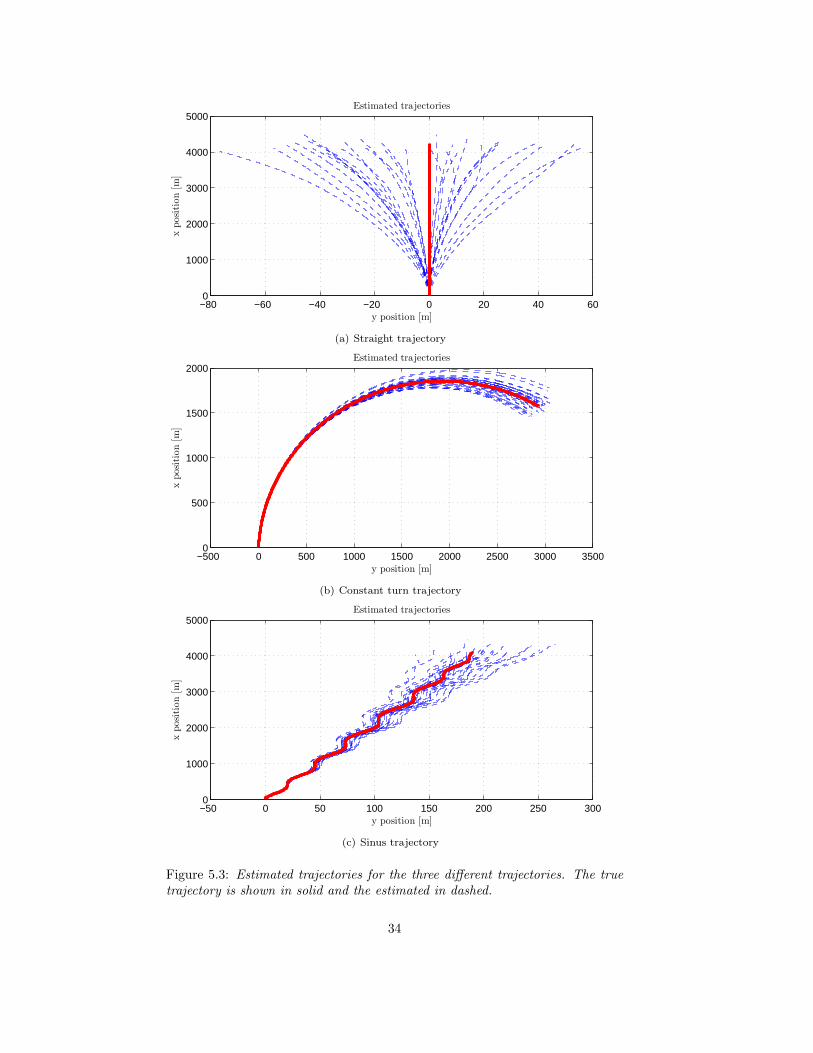
5.1.2 Impact of IMU errors on position estimation

One interesting aspect to study is how the IMU errors affects the estimationof the position. The position is estimated with the IMU equations for thethree trajectories and with IMU-errors. 30 simulations are performed for thethree trajectories respectively. In figure 5.3 the estimated position and the truetrajectory is shown. It is clearly seen that the IMU-errors are accumulatedand the position errors grows larger and larger. It is also seen that the errorsfrom the sampling of the system is small compared to the estimation errorsoriginating from the IMU errors. The same behavior is achieved for the EKFand UKF if they are not set to estimate the IMU-errors.

33

−80 −60 −40 −20 0 20 40 600

1000

2000

3000

4000

5000

y position [m]

xposi

tion

[m]

Estimated trajectories

(a) Straight trajectory

−500 0 500 1000 1500 2000 2500 3000 35000

500

1000

1500

2000

y position [m]

xposi

tion

[m]

Estimated trajectories

(b) Constant turn trajectory

−50 0 50 100 150 200 250 3000

1000

2000

3000

4000

5000

y position [m]

xposi

tion

[m]

Estimated trajectories

(c) Sinus trajectory

Figure 5.3: Estimated trajectories for the three different trajectories. The truetrajectory is shown in solid and the estimated in dashed.

34

5.1.3 Impact of model errors on position estimation

Another interesting aspect is how the model errors affect true position of themissile. With no IMU errors 30 simulations are performed with all model errorsincluded. This is preformed for the three basic trajectories and the result areshown in figure 5.4. We can see that the error induced by the measurementerrors gives are about the same size as the errors induces by the model errors.

35

−40 −30 −20 −10 0 10 20 30 400

1000

2000

3000

4000

5000

y position [m]

xposi

tion

[m]

Estimated trajectories

(a) Straight trajectory

−500 0 500 1000 1500 2000 2500 3000 35000

500

1000

1500

2000

2500

y position [m]

xposi

tion

[m]

Estimated trajectories

(b) Constant turn trajectory

−50 0 50 100 150 200 2500

1000

2000

3000

4000

5000

y position [m]

xposi

tion

[m]

Estimated trajectories

(c) Sinus trajectory

Figure 5.4: Trajectories for the missile with all model errors. The true trajectoryis shown in dashed and the nominal trajectory without any model errors areshown in solid.

36

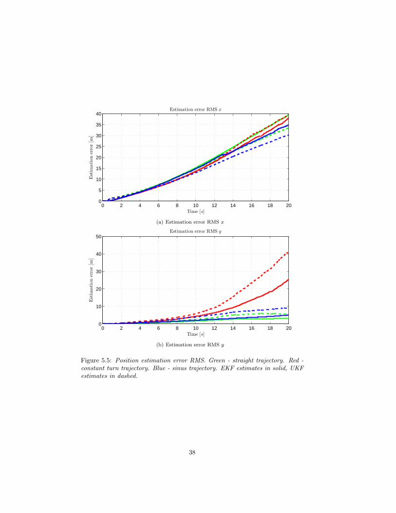
5.1.4 Comparison between EKF and UKF

The position estimation performance and the convergence of the states for theExtended Kalman filter and the Unscented Kalman filter is studied. In fig-ure 5.5 the position estimates for the three trajectories with all model errorsand measurement errors are shown both for the UKF and the EKF. It can beseen that the performance for the two filters only differs marginally. The EKFseems to have a little bit better performance. The states convergence are alsoabout the same. But the execution time is about 4 times longer for the UKFthan for the EKF. Because of these two reasons, in the analysis that follows,the EKF will be used. In a few cases in the following analysis the UKF alsois used to verify that the performance are about the same. It has been seenthat the performance is about the same for all tested cases. From this we canconclude that the non-linearities in this system is on a form so that they can beapproximated good by a first order approximation.

37

0 2 4 6 8 10 12 14 16 18 200

5

10

15

20

25

30

35

40Estimation error RMS x

Time [s]

Est

imati

on

erro

r[m

]

(a) Estimation error RMS x

0 2 4 6 8 10 12 14 16 18 200

10

20

30

40

50Estimation error RMS y

Time [s]

Est

imati

on

erro

r[m

]

(b) Estimation error RMS y

Figure 5.5: Position estimation error RMS. Green - straight trajectory. Red -constant turn trajectory. Blue - sinus trajectory. EKF estimates in solid, UKFestimates in dashed.

38

5.1.5 Observability of model errors

In this section the observability of the model errors are examined. Since thesystem are nonlinear the method to calculate the observability for linear sys-tems can not be used. Observability for nonlinear systems are much harderand therefore the observability will be studied in an practical approach. Somediscussions on observability for nonlinear systems can be found in [17]. Oneerror at a time is examined and the other model errors are set to zero. Themeasurement errors and wind turbulence are also set to zero. The ExtendedKalman filter on the other hand is initialized as if all errors were present. Fromthese simulations conclusions are drawn about the observability of the specificmodel error. Is it observable or only jointly observable with another state? Thethree different trajectories influence on the observability is also studied.

As a reference, simulations for the three trajectories with no model errorsare performed. For all three trajectories the estimation errors are small. Forthe model error parameters and IMU error parameters the largest estimationerror is smaller than 10−5.

Error in constant drag parameter CT0

We start by studying the influence on the estimation with an error in CT0. Thescale factor error for this parameter is set to 1.2. In figure 5.6 the estimationerror is ploted for three states. All other states estimates are small and are notshown here. In the first 0.3 s when the motor have not yet ignited the error inCT0 is instead compensated for in the accelerometer bias. This is because theKalman filter can not tell these errors apart. After the motor have ignited theestimation errors for the constant turn trajectory and sinus trajectory becomessmall. But the estimation error for the straight trajectory does not converge.This is due to that for the straight trajectory the terms ST0 and Sp∞

onlyappears as a factor in the model, i.e. ST0 · Sp∞

. Multiplying the estimation forthese two parameters gives approximately 1.2 which was the estimation errorfor CT0. Hence the estimations does not need to converge to the correct value.The error in one parameter could be distributed over multiple parameters. Thebetter convergence for the two other trajectories is due to that the parameterSp∞

appears before all aerodynamic parameters and for these two trajectoriesmultiple aerodynamic parameters are non zero.

39

0 1 2 3 4 5 6 7 8 9 10 11 12 13 14 15 16 17 18 19 20−0.2

−0.175

−0.15

−0.125

−0.1

−0.075

−0.05

−0.025

0Estimation error ST0

Time [s]

Est

imati

on

erro

r

(a) Estimation error ST0

0 1 2 3 4 5 6 7 8 9 10 11 12 13 14 15 16 17 18 19 200

0.01

0.02

0.03

0.04

0.05

0.06

0.07

0.08Estimation error Sp∞

Time [s]

Est

imati

on

erro

r

(b) Estimation error Sp∞

0 1 2 3 4 5 6 7 8 9 10 11 12 13 14 15 16 17 18 19 20−0.07

−0.06

−0.05

−0.04

−0.03

−0.02

−0.01

0

0.01Estimation error abiasx

Time [s]

Est

imati

on

erro

r[m/s2

]

(c) Estimation error abiasx

Figure 5.6: State estimation errors. The straight trajectory in green, the con-stant turn in red and dashed and the sinus trajectory in blue.

40

Error in the air density p∞

A scale factor error in the air density gives almost the same result as in the scalefactor in CT0 with the difference that the results for ST0 and Sp∞

are swapped.

Error in missile mass

A scale factor error in the mass is introduced. The error is set to Sm = 1.01. Infigure 5.7 the estimation of the mass scale factor error is shown. In this case theerror does not converge to zero for any trajectory. From this we can concludethat the mass is not observable. The estimation error for the position is stillsmall and thus the estimator can handle the error in the mass. The error isinstead handled mainly in ST0, SFm and Sp∞

. Since the error is not observablethe error in the mass could instead be included in the other states to reduce thesize of the model.

0 1 2 3 4 5 6 7 8 9 10 11 12 13 14 15 16 17 18 19 20−10

−9.9

−9.8

−9.7

−9.6

−9.5

−9.4

−9.3x 10

−3 Estimation error Sm

Time [s]

Figure 5.7: Mass scale factor estimation error. The straight trajectory in green,the constant turn in red and dashed and the sinus trajectory in blue.

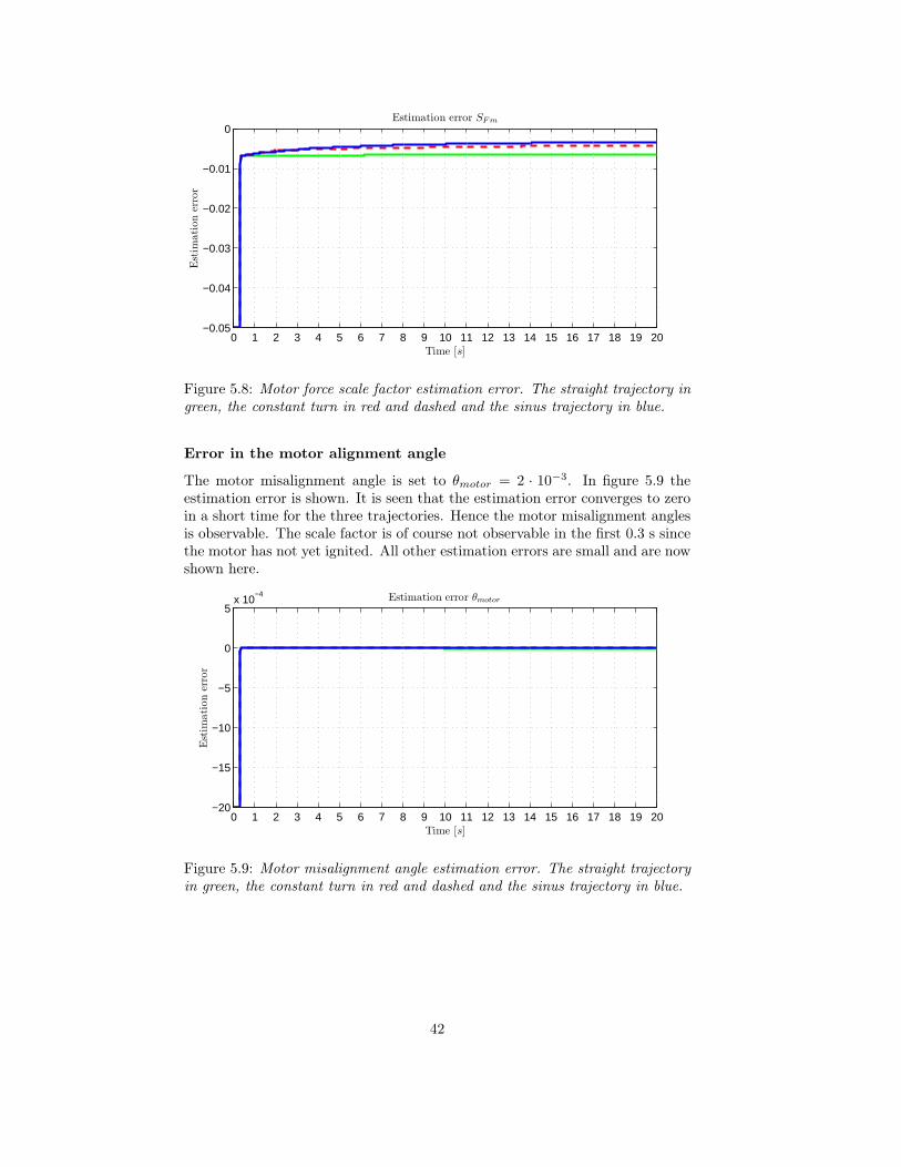
Error in the force generated by the motor

The scale factor error for the motor force is set to SFm = 1.05. In figure 5.8 theestimation error is shown for the three trajectories. The estimator has aboutthe same performance for the three trajectories. A large part of the scale factorerror is found by the EKF but not all. In the previous cases the remaining errorhas been handled in other state estimates, but this is not the case here. Otherstates are affected but a significant error in the position estimate is obtained.From this we can conclude that this parameter is hard to observe.

41

0 1 2 3 4 5 6 7 8 9 10 11 12 13 14 15 16 17 18 19 20−0.05

−0.04

−0.03

−0.02

−0.01

0Estimation error SF m

Time [s]

Est

imati

on

erro

r

Figure 5.8: Motor force scale factor estimation error. The straight trajectory ingreen, the constant turn in red and dashed and the sinus trajectory in blue.

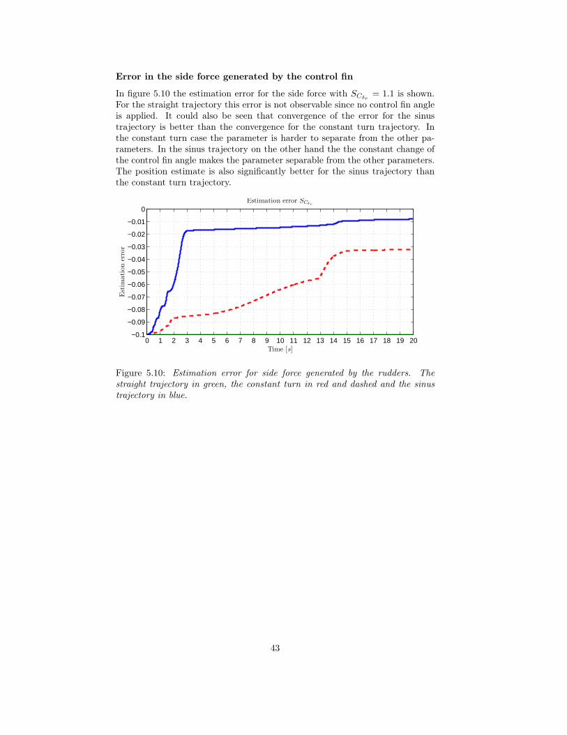
Error in the motor alignment angle

The motor misalignment angle is set to θmotor = 2 · 10−3. In figure 5.9 theestimation error is shown. It is seen that the estimation error converges to zeroin a short time for the three trajectories. Hence the motor misalignment anglesis observable. The scale factor is of course not observable in the first 0.3 s sincethe motor has not yet ignited. All other estimation errors are small and are nowshown here.

0 1 2 3 4 5 6 7 8 9 10 11 12 13 14 15 16 17 18 19 20−20

−15

−10

−5

0

5x 10

−4 Estimation error θmotor

Time [s]

Est

imati

on

erro

r

Figure 5.9: Motor misalignment angle estimation error. The straight trajectoryin green, the constant turn in red and dashed and the sinus trajectory in blue.

42

Error in the side force generated by the control fin

In figure 5.10 the estimation error for the side force with SCδr= 1.1 is shown.

For the straight trajectory this error is not observable since no control fin angleis applied. It could also be seen that convergence of the error for the sinustrajectory is better than the convergence for the constant turn trajectory. Inthe constant turn case the parameter is harder to separate from the other pa-rameters. In the sinus trajectory on the other hand the the constant change ofthe control fin angle makes the parameter separable from the other parameters.The position estimate is also significantly better for the sinus trajectory thanthe constant turn trajectory.

0 1 2 3 4 5 6 7 8 9 10 11 12 13 14 15 16 17 18 19 20−0.1

−0.09

−0.08

−0.07

−0.06

−0.05

−0.04

−0.03

−0.02

−0.01

0Estimation error SCδr

Time [s]

Est

imati

on

erro

r

Figure 5.10: Estimation error for side force generated by the rudders. Thestraight trajectory in green, the constant turn in red and dashed and the sinustrajectory in blue.

43

Error in the moment generated by the control fin

The scale factor error Snδris set to 1.1. In figure 5.11 the estimation error for

the moment generated by the rudder is shown. Again, for the same reason givenabove, the scale factor error is not observable for the straight trajectory. For thetwo other trajectories on the other hand it is observable and the error convergesto zero. All other parameter errors are small and the position estimate error isalso small.

0 1 2 3 4 5 6 7 8 9 10 11 12 13 14 15 16 17 18 19 20−0.1

−0.09

−0.08

−0.07

−0.06

−0.05

−0.04

−0.03

−0.02

−0.01

0

0.01Estimation error Snδr

Time [s]

Est

imati

on

erro

r

Figure 5.11: Estimation error for the moment generated by the control fin. Thestraight trajectory in green, the constant turn in red and dashed and the sinustrajectory in blue.

44

Error in the side force due to the sideslip angle

The scale factor error for the side force from the sideslip angle is set to SCβ= 1.1.

In figure 5.12 the estimation error is shown. For the straight trajectory thesideslip angle is zero and the state is not observable. The estimate for both theconstant turn and the sinus trajectory converges but with a static error. Theremaining error is not completely handled in other states and a larger error isobtained in the position estimates.

0 1 2 3 4 5 6 7 8 9 10 11 12 13 14 15 16 17 18 19 20−0.1

−0.09

−0.08

−0.07

−0.06

−0.05

−0.04

−0.03

−0.02

−0.01

0

0.01Estimation error SCβ

Time [s]

Est

imati

on

erro

r

Figure 5.12: Estimation error in the side force due to sideslip angle. The straighttrajectory in green, the constant turn in red and dashed and the sinus trajectoryin blue.

45

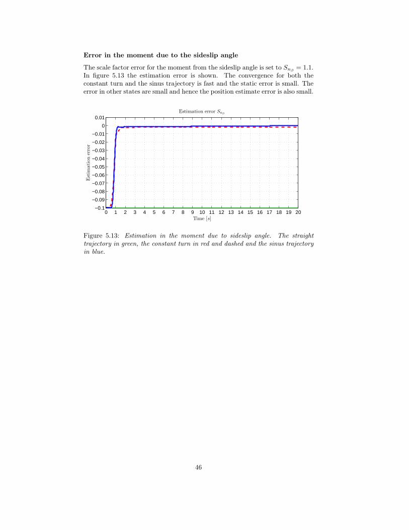
Error in the moment due to the sideslip angle

The scale factor error for the moment from the sideslip angle is set to Snβ= 1.1.

In figure 5.13 the estimation error is shown. The convergence for both theconstant turn and the sinus trajectory is fast and the static error is small. Theerror in other states are small and hence the position estimate error is also small.

0 1 2 3 4 5 6 7 8 9 10 11 12 13 14 15 16 17 18 19 20−0.1

−0.09

−0.08

−0.07

−0.06

−0.05

−0.04

−0.03

−0.02

−0.01

0

0.01Estimation error Snβ

Time [s]

Est

imati

on

erro

r

Figure 5.13: Estimation in the moment due to sideslip angle. The straighttrajectory in green, the constant turn in red and dashed and the sinus trajectoryin blue.

46

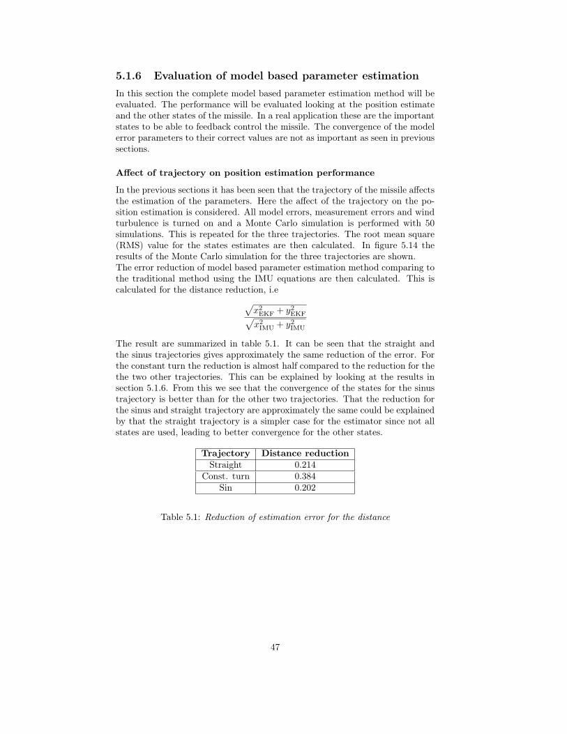
5.1.6 Evaluation of model based parameter estimation

In this section the complete model based parameter estimation method will beevaluated. The performance will be evaluated looking at the position estimateand the other states of the missile. In a real application these are the importantstates to be able to feedback control the missile. The convergence of the modelerror parameters to their correct values are not as important as seen in previoussections.

Affect of trajectory on position estimation performance

In the previous sections it has been seen that the trajectory of the missile affectsthe estimation of the parameters. Here the affect of the trajectory on the po-sition estimation is considered. All model errors, measurement errors and windturbulence is turned on and a Monte Carlo simulation is performed with 50simulations. This is repeated for the three trajectories. The root mean square(RMS) value for the states estimates are then calculated. In figure 5.14 theresults of the Monte Carlo simulation for the three trajectories are shown.The error reduction of model based parameter estimation method comparing tothe traditional method using the IMU equations are then calculated. This iscalculated for the distance reduction, i.e

√

x2EKF

+ y2EKF

√

x2IMU

+ y2IMU

The result are summarized in table 5.1. It can be seen that the straight andthe sinus trajectories gives approximately the same reduction of the error. Forthe constant turn the reduction is almost half compared to the reduction for thethe two other trajectories. This can be explained by looking at the results insection 5.1.6. From this we see that the convergence of the states for the sinustrajectory is better than for the other two trajectories. That the reduction forthe sinus and straight trajectory are approximately the same could be explainedby that the straight trajectory is a simpler case for the estimator since not allstates are used, leading to better convergence for the other states.

Trajectory Distance reduction

Straight 0.214Const. turn 0.384

Sin 0.202

Table 5.1: Reduction of estimation error for the distance

47

0 1 2 3 4 5 6 7 8 9 10 11 12 13 14 15 16 17 18 19 200

25

50

75

100

125

150Estimation error RMS x

Time [s]

Est

imati

on

erro

r[m

]

(a) Estimation error RMS x

0 1 2 3 4 5 6 7 8 9 10 11 12 13 14 15 16 17 18 19 200

10

20

30

40

50

60

70

80Estimation error RMS y

Time [s]

Est

imati

on

erro

r[m

]

(b) Estimation error RMS y

Figure 5.14: Affect of trajectory on position estimates. The straight trajectory ingreen, the constant turn in red and the sinus trajectory in blue. EKF estimatesin solid, estimates from IMU equations in dashed.

48

Varying the motor ignition time

The time from the missile leaves the tube until the motor ignites could easily bevaried. The affect of this time on the performance will be studied. It could bethat some states converges faster during this time before the motor ignites andthat this will improve performance. This time is set to zero and to 3 secondsrespectively. Monte Carlo simulations are then performed for the two cases.Studying the results from the simulations gives that the performance for thetwo cases are about the same. Only the bias for the x accelerometer convergesunder the three seconds before the motor ignites. All other states seems to beunobservable during this time. The accelerometer bias converges fast in theother case and hence the performance for the two cases are approximately thesame.

Affect of measurement errors on position estimation

The size of the measurement errors are determined by the quality of the IMUused in the application. But it could be interesting to see how much the size ofthe IMU errors affects the position estimation. This information could be used todecide if a worse or better IMU should be used and how much performance thatis gained or lost from this. The standard deviation for the meassurment errorsare set to three times the normal standard deviation. The initlization of theKalman filter is then altered. Monte Carlo simulations are performed for a fewcases and the result are compared to the result using the normal measurementerrors. The trajectory is chosen to the constant turn trajectory. In figure 5.15the result of the Monte Carlo simulation is shown. The results for the two caseswith larger measurement errors are about the same. This indicates that thefilter is not perfectly tuned. It might be possible to increase the performanceif the filter is better tuned. Comparing the results for the original standarddeviation with the large standard deviation it is seen that the performance forthe EKF does not decrease in the same extent as the traditional method usingthe IMU equations.

49

0 1 2 3 4 5 6 7 8 9 10 11 12 13 14 15 16 17 18 19 200

20

40

60

80

100

120

140

160Estimation error RMS in velocity vector direction

Time [s]

Est

imati

on

erro

r[m

]

(a) Position estimation error RMS in velocity direction.

0 1 2 3 4 5 6 7 8 9 10 11 12 13 14 15 16 17 18 19 200

50

100

150

200

250

300Estimation error RMS orthogonal to velocity vector

Time [s]

Est

imati

on

erro

r[m

]

(b) Position estimation error RMS orthogonal to the velocity vector direction.

Figure 5.15: Affect of measurement errors on position estimates in the velocitydirection and orhogonal to the velocity vector. Normal meassurment errors andEKF initialized as normal in green. Three times as large meassurment errorsand EKF initialized as normal in red. Three times as large meassurment errorsand EKF initialized correctly in blue. EKF estimates in solid, estimates fromIMU equations in dashed.

50

Affect of model errors on position estimation

Another interesting aspect is how the size of the model errors affect the po-sition estimation performance. This gives some idea about the robustness ofthe method. The standard deviation for the model errors are set to five timethe normal standard deviation. First without increasing the initial state errorcovariance matrix and then by give the matrix its correct values. Monte Carlosimulations are then performed for the different cases and the result are com-pared to result using the normal model errors. The results are presented infigure 5.16. In the figure it can be seen that the for the case where the EKF iscorrectly initialized the performance are only slightly worse for the case were thesize of the model errors has been increased. But for the case where the modelerrors are increased but the filter is not correctly initialized the performancehas deteriorated significantly. In the case where initial state error covariancematrix is set to a larger value than the acctual model errors the performanceis about the same as for the case with the large model error and the correctinitial covariance for the filter. From this we can conclude that it is importantto know the size of the model errors to be able to correctly initialize the filter. Ainitial value of the state error covariance matrix chosen to small deteriorates theperformance significantly. But value chosen to large will give the performanceas if the model errors actual were that size as chosen in the initial covariancematrix.

Affect of wind turbulence on position estimation performance

The affect of the size of the wind turbulence on the estimation will be examinedin this section. Again the constant turn trajectory is used and the the windturbulence is set to three times. The EKF initialization values are then altered.This setup is then simulated using Monte Carlo simulation with 50 simulationsfor each case. The result is shown in figure 5.17. It is seen that the windturbulence only has a small impact on the estimation performance for all caseswithout the case where the wind turbulence is three times larger than normaland the Kalman filter is initialized to one third of normal wind turbulence.From this we can conclude that the EKF probably is initialized with a toolarge process noise covariance since the performance does not change when theturbulence is increased and the Kalman filter is initialized as normal. When theprocess noise covariance is lowered on the other hand and the wind turbulenceis increased the performance deteriorates.

51

0 1 2 3 4 5 6 7 8 9 10 11 12 13 14 15 16 17 18 19 200

10

20

30

40

50

60

70

80

90

100Estimation error RMS x

Time [s]

Est

imati

on

erro

r[m

]

(a) Estimation error RMS x

0 1 2 3 4 5 6 7 8 9 10 11 12 13 14 15 16 17 18 19 200

10

20

30

40

50

60

70

80

90Estimation error RMS y

Time [s]

Est

imati

on

erro

r[m

]

(b) Estimation error RMS y

Figure 5.16: Affect of model errors on position estimates. Green - normal modelerrors, EKF initialized correctly. Red - 5x normal model errors, EKF initial-ized with normal model errors. Blue- 5x normal model errors, EKF initializedcorrectly. Yellow - normal model errors, EKF initialized for 5x normal modelerrors. EKF estimates in solid, estimates from IMU equations in dashed.

52

0 1 2 3 4 5 6 7 8 9 10 11 12 13 14 15 16 17 18 19 200

10

20

30

40

50

60

70

80

90

100Estimation error RMS x

Time [s]

Est

imati

on

erro

r[m

]

(a) Estimation error RMS x

0 1 2 3 4 5 6 7 8 9 10 11 12 13 14 15 16 17 18 19 200

10

20

30

40

50

60

70

80

90

100

110Estimation error RMS y

Time [s]

Est

imati

on

erro

r[m

]

(b) Estimation error RMS y

Figure 5.17: Affect of wind turbulence on position estimates. Green - normalwind turbulence, EKF initialized correctly. Red - 3x normal wind turbulence,EKF initialized for normal wind turbulence. Blue- 3x normal wind turbulence,EKF initialized correctly. Yellow - 3x normal wind turbulence, EKF initializedfor 1/3x normal wind turbulence. EKF estimates in solid, estimates from IMUequations in dashed.

53

5.1.7 Added positioning sensor

To evaluate the missile in real life, test fires of the missile is performed undercontrolled circumstances. During these tests more information is available frommultiple sensors. Here the effect of adding a positioning sensor will be studied.By combining the measurements from the positioning sensor and the IMU mea-surements in an estimator, more information about the states could be gained.This information could be used to evaluate the missile and be used in trou-bleshooting if something has gone wrong in the test. In this case the interestingpart is not to study the position estimate, since the position is measured, butthe actual convergence of the states to their real values.

Another interesting aspect of adding a positioning sensor is if it can be usedfor a short period of time in the beginning of the flight to get the states toconverge. After this the position measuring is turned off and we have the samecase as before. But after this better performance should be gained since thestates estimates is better than without the initial position measurement. Thiscould be the case if only an short range positioning sensor is available. It istherefore important to see how long time it takes for the states to convergeand what happens after the positioning measurements are lost. In this case theposition estimate will be studied.

Here we assume that the position of the missile is measured with a radar. Theradar does not directly give the position in cartesian coordinates but measuresthe distance and angle to the missile. The radar measurement are disturbed bymeasurement noise. This gives two more measurement equations.

rradar =√

x2 + y2 + wr (5.1.1a)

θradar = arctan(y

x

)

+ wθ (5.1.1b)

where rradar is the measured distance to the missile, θradar is the measured angleto the missile and wr and wθ are zero mean independent white noise processewith standard deviation 10 m and 1 mrad respectevly.

We start by looking at the convergence and convergence time for the states.Monte Carlo simulations are performed for the three different trajectories withposition measurements. In figure 5.18 a couple of interesting states are ploted.Generally the convergence for the most states for all the three trajectories arebetter than without the position sensor. Again the convergence for the sinustrajectory is the best. The scale factor error for the mass is still not observablefor any of the three trajectories.

54

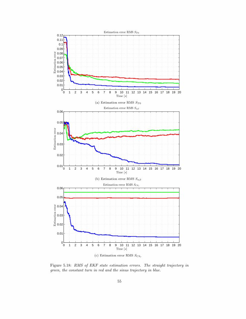
0 1 2 3 4 5 6 7 8 9 10 11 12 13 14 15 16 17 18 19 200

0.01

0.02

0.03

0.04

0.05

0.06

0.07

0.08

0.09

0.1

0.11

0.12Estimation error RMS ST0

Time [s]

Est

imati

on

erro

r

(a) Estimation error RMS ST0

0 1 2 3 4 5 6 7 8 9 10 11 12 13 14 15 16 17 18 19 200.01

0.02

0.03

0.04

0.05

0.06Estimation error RMS Snβ

Time [s]

Est

imati

on

erro

r

(b) Estimation error RMS Snβ

0 1 2 3 4 5 6 7 8 9 10 11 12 13 14 15 16 17 18 19 200

0.01

0.02

0.03

0.04

0.05

0.06Estimation error RMS SCδr

Time [s]

Est

imati

on

erro

r

(c) Estimation error RMS SCδr

Figure 5.18: RMS of EKF state estimation errors. The straight trajectory ingreen, the constant turn in red and the sinus trajectory in blue.

55

Looking at the state convergence time a majority of the states have convergedto a large part of their final value in about two-three seconds. This time canbe used for the test were the position sensor only is used in the beginningof the trajectory. The sinus trajectory will also be used in this test since itgives the best performance. Monte Carlo simulations are performed for a fewdifferent position measuring times. The times are 1 s, 2 s, 4 s and 6 s chosenfrom the convergence time as a starting point. The results of the Monte Carlosimulations are presented in figure 5.19. In the figure it is seen that result for

0 1 2 3 4 5 6 7 8 9 10 11 12 13 14 15 16 17 18 19 200

5

10

15

20

25

30

35Estimation error RMS x

Time [s]

Est

imati

on

erro

r[m

]

(a) Estimation error RMS x

0 1 2 3 4 5 6 7 8 9 10 11 12 13 14 15 16 17 18 19 200

1

2

3

4

5Estimation error RMS y

Time [s]

Est

imati

on

erro

r[m

]

(b) Estimation error RMS y

Figure 5.19: EKF position estimation error RMS. Position measurement time:green 0 s, blue 1 s, green 2 s, yellow 4 s and cyan 6 s.

the case with position measurement for 1 s is about the same as the result forthe case without position measurements. From this it can be concluded that thestates has not converged enough to affect the performance. For 2 s, 4 s and 6 sposition measuring the performance is better. The 2 s case only gives a smallperformance increase while the 4 s case increases the performance significantly.The performance gain between 4 s and 6 s is not as large as the performance

56

gain comparing 2 s and 4 s. From this it can be concluded that the states haveconverged most part of their final value in 4 s and that this time could be areasonable time for position measurement to improve performance. This is thecase even if the position estimates are compared so that the position estimatesare compared for equal times after the position measuring is stopped.

5.2 Simulations in three dimensions

The simulations performed in three dimensions are only used to verify the func-tion of the model based parameter estimation method for the missile. A thor-ough analysis of the results will not be performed because of the many statesand the time consuming simulations. The parameter values given in appendix Aare used. Monte Carlo simulations are carried out for three different cases. Thefirst case is the straight trajectory, but with the different now that the gravityaffects the missile. The second case is the straight trajectory but the missilerolls slowly. The last case simulated is a case were the missile is slowly ascend-ing. The RMS value for the Monte Carlo simulations are calculated and shownin figure 5.20.

57

0 1 2 3 4 5 6 7 8 9 10 11 12 13 14 15 16 17 18 19 200

102030405060708090

100110120130

Estimation error RMS x

Time [s]

Est

imati

on

erro

r[m

]

(a) Estimation error RMS x

0 1 2 3 4 5 6 7 8 9 10 11 12 13 14 15 16 17 18 19 200

5

10

15

20

25

30

35

40Estimation error RMS y

Time [s]

Est

imati

on

erro

r[m

]

(b) Estimation error RMS y

0 1 2 3 4 5 6 7 8 9 10 11 12 13 14 15 16 17 18 19 200

10

20

30

40

50

60Estimation error RMS z

Time [s]

Est

imati

on

erro

r[m

]

(c) Estimation error RMS z

Figure 5.20: RMS of state estimation errors. The straight trajectory in green,the straight trajectory with a slow roll in red and the slow ascending trajectoryin blue. EKF estimates in solid, estimates from IMU equations in dashed.

58

It can be seen that the method also works in three dimensions. The methodstill gives significantly better results than the traditional method. The stateconvergence for the other states are about the same as in two dimensions.

59

Chapter 6

Conclusions and future work

6.1 Conclusions

Throughout this report it has been shown that increased performance is gainedby using the model based parameter estimation method instead of the traditionalnavigation equations. The most important aspect of the performance gain is thesize of the model errors compared to the size of the measurement errors.

Two different estimators were considered the Extended Kalman filter andthe Unscented Kalman filter. It has been shown that the EKF and the UKFgives about the same performance but the execution time for the UKF werelonger. However the the estimators were not implemented optimally and an-other implementation could give other execution times. From this it can beconcluded that the missile system implemented here, is approximated well bylinear approximation used by the EKF. It can also be concluded that the per-formance when estimating the position is not estimator dependent but is moreabout the basic observability of the system.

Observability for a non linear system are not as easily analyzed as a linearsystem. In the missile model we have states that are only observable jointlywith other states. Not all states converges to their true value but the error isinstead caught in other state estimates. This can be seen in the analysis thatwere performed with one model error at a time. It can also been seen by thefact that the states in many cases does not converge but the state estimationfor the position is still quite good.

The performance and observability of the states are dependent on the tra-jectory. The trajectory both affects the impact of the IMU-errors and on theobservability. The best performance is achieved for the sinus trajectory becauseof its excitation of the states. This knowledge might be used to improve theperformance for all trajectories. A sinus input could added on top on the de-sired trajectory or a sinus trajectory could be used in the beginning of the flightand when the states has converged the missile is steered along another trajec-tory. Because of the constant turning back and forth with the sinus input themissile loses energy and consequently loses range compared to a trajectory withless turning. But if this leads to better position estimation the actual practicalrange could instead be increased. This also shows the need for consider the es-timation when designing the midcourse guidance system to choose trajectories

60

that improves the state estimation.The evaluation with a added position sensor has shown that it is possible

to increase the estimation performance if the position is measured for a shortperiod of time in the beginning of the trajectory. The states converges muchbetter using the position sensor than without it and this method could be usedin the evaluation of fired missiles in controlled circumstances.

In this report the estimator model and the simulation model has had thesame structure but with different parameter values. In a real application itcould be hard to model the system to the same extent to get the same structure.This will probably deteriorate the performance for the estimates. This is onething that needs to be looked into before a real implementation could be made.But with this said, the model based parameter estimation method evaluated inthis report has potential to improve the position estimation also in a real missileapplication.

6.2 Future work

Before this method could be used in an real implementation more studies mustbe done. The main thing to do is to try the method with data from realmissiles. The model here has used a few simplifications as for example thelinearization of the aerodynamics. From the real missile data this model needsto be verified and there might be a need to add other states or remove somestates. More analysis of the three dimensional case is also necessary before animplementation. The tuning of the filter has been done by a very simple methodas shown in section 4.2.4. Better performance could almost certain be gainedby tuning the filters.

61

Bibliography

[1] Chowdhary, Girish and Jategaonkar, Ravindra Aerodynamic Pa-rameter Estimation from Flight Data Applying Extended and UnscentedKalman Filter DLR Institute for Flight System, Braunschweig, Germany,2006, AIAA 2006-6146.

[2] Shareef, Haider Gyrobiasskattning för små autonoma flygplan. TekniskaHögskolan i Linköping. Linköping 2007. Examensarbete.

[3] Ankelhed,Daniel and Stenlind, Lars Tillståndsskattning i robotmod-ell med accelerometrar. Tekniska Högskolan i Linköping. Linköping 2005.Examensarbete.

[4] Zipfel, Peter H. Modeling and simulation of aerospace vehicle dynamics.American Institute of Aeronautics and Astronautics 2007, 2nd Edition.

[5] Meriam, J. L. and Kraige, L. G. Engineering mechanics: Dynamics.Wiley 2007, 6th Edition.

[6] Bertin, John J. and Smith, Michael L. Aerodynamics for engineers.Prentice Hall 1998, 3rd Edition.

[7] Boiffier, Jean-Luc The Dynamics of Flight: the Equations. Wiley 1998.

[8] US. Department of Defence Flying Qualities of Piloted Aircraft. MIL-HDBK-1797. 19 december 1997

[9] Hjalmarsson, Håkan och Ottersten, Björn Lecture Notes in Adap-tive Signal Processing. Kungl tekniska högskolan. Instutitionen för Signaler,Sensorer & System. 2002

[10] Bozic, S.M. Digital and Kalman Filtering: An Introduction to Discrete-Time Filtering and Optimum Linear Estimation. Arnold 1994, 2nd Edition.

[11] Brown, Robert Grover and Hwang, Patrick Y. C. Introductionto random signals and applied Kalman filtering with Matlab Exercises andSolutions. Wiley 1997, 3rd Edition.

[12] Julier, Simon J. and Uhlmann, Jefferey K. A New Extension of theKalman Filter to Nonlinear Systems. SPIE AeroSense Symposium, April21-24, 1997.

62

[13] Hendeby, Gustaf Performance and Implementation - Aspects of Non-linear Filtering. Division of Automatic Control, Department of ElectricalEngineering, Linköping University. 2008ISBN 978-91-7393-979-9

[14] Glad, Torkel and Ljung, Lennart Control theory : Multivariable andNonlinear Methods. Taylor & Francis, 2000

[15] Van Loan, Charles F Computing Integrals Involving the Matrix Expo-nential. IEEE Transactions on Automatic Control, vol.23, no.3, p. 395-404,june 1978

[16] Eriksson,Gerd Numeriska algoritmer med MATLAB. NADA, KTH.June 2002.

[17] Hermann, Robert and Krener,Arthur J. Nonlinear Controllabilityand Observability. IEEE Transactions on Automatic Control Vol. Ac-22,No 5, October 1977.

63

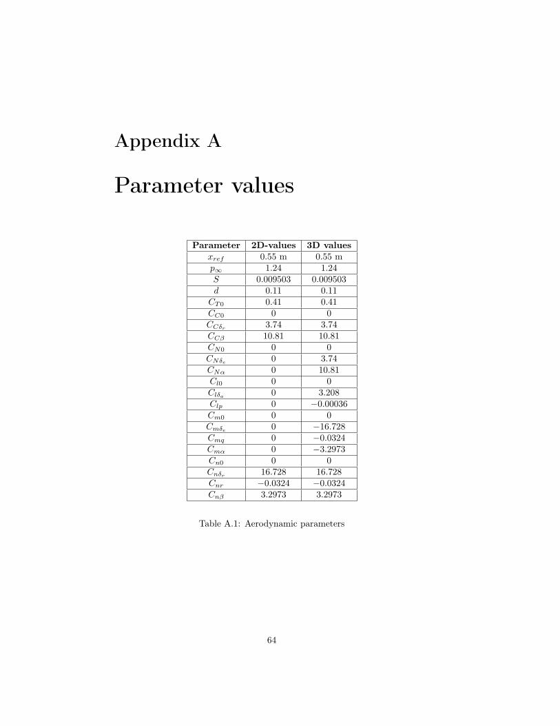
Appendix A

Parameter values

Parameter 2D-values 3D values

xref 0.55 m 0.55 mp∞ 1.24 1.24S 0.009503 0.009503d 0.11 0.11CT0 0.41 0.41CC0 0 0CCδr

3.74 3.74CCβ 10.81 10.81CN0 0 0CNδe

0 3.74CNα 0 10.81Cl0 0 0Clδa

0 3.208Clp 0 −0.00036Cm0 0 0Cmδe

0 −16.728Cmq 0 −0.0324Cmα 0 −3.2973Cn0 0 0Cnδr

16.728 16.728Cnr −0.0324 −0.0324Cnβ 3.2973 3.2973

Table A.1: Aerodynamic parameters

64

Parameter 2D-values 3D values

Ixx 0.027 kgm2 0.027 kgm2

Iyy 0.95 kgm2 0.95 kgm2

Izz 0.96 kgm2 0.96 kgm2

xc 0.56 m 0.56 myc 0 m 0 mzc 0 m 0 mg 0 9.81m/s

Table A.2: Missile parameters

Parameter Values

Ib 1475 NsIs 2400 Nstb 0.5 sts 12 smb 0.74 kgms 1.39 kgmtot 12 kgtign 0.3 sτm 0.05 s

Table A.3: Motor parameters

Parameter 2D-values 3D values

σSFm0.025 0.025

σφmotor10−3 10−3

σϕmotor10−3 10−3

σSlδa0 0.05

σSCδr0.05 0.05

σSnδr0.05 0.05

σSNδe0 0.05

σSmδe0 0.05

σSnβ0.05 0.05

σSCβ0.05 0.05

σSmα0 0.05

σSNα0 0.05

σSCT00.1 0.1

σSp∞

0.075 0.075σSm

0.005 0

Table A.4: Model parameter uncertainties

65

Parameter 2D-values 3D values

σbiasx0.6 0.6

σbiasy0.16 0.16

σbiasz0 0.16

σbiasp0 0.001

σbiasq0 0.001

σbiasr0.001 0.001

σSax0.008 0.008

σSay0.00426 0.00426

σSaz0 0.00426

σSωp0 0.003

σSωq0 0.003

σSωr0.003 0.003

Table A.5: IMU errors

Parameter 2D-values 3D values

h 15 m 15 mv 140 m/s 140 m/sσz 1.6 m/s 1.6 m/sσwcx

2.5 m/s 2.5 m/sσwcy

2.5 m/s 2.5 m/sσwcz

0 m/s 2.5 m/s

Table A.6: Wind parameters

66