{Model Checking and Static Analysis of Intel MCS-51 - Wien

DIPLOMA THESISfor an academic degree

"Master of Science in Engineering"

Model Checking and Static Analysis ofIntel MCS-51 Assembly Code

by Thomas Reinbacher, BScA-2020 Kleinstelzendorf, Weidenweg 44

1. Examiner: FH-Prof. Dipl.-Ing. Dr. Martin Horauer2. Examiner: Ing. Dipl.-Ing. Michael KramerVienna, June 3rd, 2009

Written at the University of Applied Sciences Technikum Wien

Master Degree Programme Embedded Systems

Affidavit

„I hereby declare by oath that I have written this paper myself. Any ideas and conceptstaken from other sources either directly or indirectly have been referred to as such. Thepaper has neither in the same nor similar form been handed in to an examination board,nor has it been published. “

Place, Date Signature

Abstract

Verification of embedded systems software is crucial for providing flawless functionality ofnowadays intelligent computer systems found in automobiles, elevators, aircrafts, medicaldevices, robots, etc. The common approach most widely used in industry relies on testingof defined corner cases. Although everyone is aware of the fact that only a very limitedset of the test space can be covered in this way, no other more complete approaches havebeen widely adopted so far.Formal verification methods such as model checking complemented with various tech-

niques to reduce state spaces has recently gained some momentum in this regard. Nev-ertheless, formal verification of embedded systems still played a minor role in the past.Practical restrictions of this approach are (i) due to the problem to (manually) create amodel of the system beforehand and (ii) due to the resulting large state spaces.This master thesis focuses on model checking and static analysis of Intel MCS-51 assem-

bly code with the [mc]square framework.In the presented approach, issue (i) is solved by using a dedicated target CPU simulator.

In order to tackle (ii) existing abstraction techniques are adapted for the Intel MCS-51 tar-get architecture. A novel state space reduction technique termed Delayed Nondeterminismwith Look Ahead is introduced. The presented abstraction technique centers around thecoherence among boolean operators with particular regard to the 3-valued microcontrollermemory model.Besides, the Intel MCS-51 CPU simulator is integrated into the existing static analysis

framework of [mc]square. A novel data-flow analysis termed Register Bank Analysis isdescribed in order to handle register bank swapping. Register bank swapping is a particularfeature of some embedded microcontrollers such as the Intel MCS-51. This approach allowsnarrowing and refining the subsequent data-flow analyses, leading to more precise analysisresults. The additional precision in turn contributes to a reduction of state spaces duringmodel checking.In order to evaluate the benefits and to show the applicability of the introduced

concepts, a real world case study is conducted. The case study source code is takenfrom an industrial application. The microcontroller software is model checked with[mc]square by taking advantage of the presented state space abstractions and staticanalysis techniques.

Keywords: Assembly code model checking, static analysis of assembly code, abstractiontechniques, case study, [mc]square

Kurzfassung

Die Verifikation von Software für Embedded Systems ist ein notwendiges Kriterium umdie fehlerfreie Funktion von intelligenten Computersystemen in Automobilen, Aufzügen,Flugzeugen, medizintechnischen Geräten, Robotern, usw. zu garantieren. Die in der In-dustrie weit verbreitete Standardmethode beruht auf dem Abdecken von einigen weni-gen repräsentativen Testfällen. Es ist bekannt, dass dieser Ansatz nur eine sehr kleineMenge des tatsächlichen Testraums abdecken kann, trotzdem gibt es nur wenig ausgereifteKonzepte um diesen Verifikationsmißstand zu beseitigen.Formale Verifikationsmethoden wie Model Checking sind vielversprechende Ansätze um

die Fehlerfreiheit von Software zu zeigen. Im Kontext von Embedded Systems spieltendiese formalen Ansätze in der Vergangenheit nur eine untergeordneter Rolle. In der Praxiszeigen sich Schwierigkeiten durch (i) die manuell durchgeführte Modellierung des Systemsund (ii) die unhandbar großen Zustandsräume.Diese Masterarbeit beschäftigt sich mit Model Checking und Statischer Analyse von

Intel MCS-51 Assembler Code unter Zuhilfenahme des [mc]square Frameworks.Der vorgestellte Ansatz versucht das Problem (i) durch einen speziellen Mikrocontroller-

simulator zu lösen. Bestehende Abstraktionstechniken werden für den Intel MCS-51 Mikro-controller angepasst um die entstehenden Zustandsräume zu minimieren (ii). Eine neueZustandsreduktion namens Delayed Nondeterminism with Look Ahead wird vorgestellt.Dieser Ansatz basiert auf den Zusammenhängen zwischen Boole’scher Logik und dem drei-wertigen Speichermodell des Mikrocontrollersimulators.Weiters wird der vorhandene Intel MCS-51 Simulator in das Statische Analyse Frame-

work von [mc]square integriert. Eine neuartige Datenflussanalyse (Register Bank Analy-sis) wird entwickelt um das architekturbedingte Umschalten von Registerbänken zu berück-sichtigen. Dieser Ansatz erlaubt es die nachfolgenden Analyseergebnisse einzugrenzen undzu präzisieren. Diese gewonnene Präzision erlaubt eine weitere Zustandsreduktion währenddes Model Checkings.Um die Vorteile und die Anwendbarkeit der vorgestellten Konzepte zu demonstrieren

wird eine Fallstudie vorgestellt. Die Software der Fallstudie stammt aus einer industriellenAnwendung. Das Mikrocontrollerprogramm wir unter Zuhilfenahme der vorgestelltenAbstraktionstechniken und statischen Analysen mit dem [mc]square Model Checkerverifiziert.

Schlagwörter: Assembler Code Model Checking, Statische Analyse von Assembler Code,Abstraktionstechniken, Fallstudie, [mc]square

Acknowledgements

Not because it is customary, but because it is appropriate: I would like to thank myadvisor, FH-Prof. Dr. Martin Horauer, for his excellent guidance and for giving me the op-portunity to join one of his research projects within the Department of Embedded Systemsat the University of Applied Sciences FH Technikum Wien. He allowed me a great degreeof freedom in my work and kindly helped me to gain ground in academic work. Most valu-able to me were his numerous tips, his pragmatic approach of doing things, and our fruitfuldiscussions both related and unrelated to work. I highly enjoyed the time working together.

Next, I want to thank Dr. Bastian Schlich and his team from the Embedded SoftwareLaboratory at the RWTH Aachen University. Even though we were most time geographi-cally separated, he greatly contributed to set up a smooth and rich collaboration. He wasalways willing to listen to my problems and gave me plenty of support to get started withmodel checking and [mc]square.

Last – but definitely not least – I thank my family and friends. They supported me ineverything I did and greatly helped me to make my way.

Thomas ReinbacherVienna, June 2009

Contents

1 Motivation and Introduction 1

2 Contribution 32.1 Status Quo . . . . . . . . . . . . . . . . . . . . . . . . . . . . . . . . . . . . 32.2 Thesis Contribution . . . . . . . . . . . . . . . . . . . . . . . . . . . . . . . 32.3 Long-Term Vision . . . . . . . . . . . . . . . . . . . . . . . . . . . . . . . . . 4

3 Background 53.1 A World Where Nothing Works and Nobody Knows Why . . . . . . . . . . 53.2 Formal Verification . . . . . . . . . . . . . . . . . . . . . . . . . . . . . . . . 63.3 The Verification Problem . . . . . . . . . . . . . . . . . . . . . . . . . . . . 73.4 Model Checking . . . . . . . . . . . . . . . . . . . . . . . . . . . . . . . . . . 8

3.4.1 The Model Checking Problem . . . . . . . . . . . . . . . . . . . . . . 93.4.2 The Kripke Structure . . . . . . . . . . . . . . . . . . . . . . . . . . 93.4.3 The Temporal Logic CTL . . . . . . . . . . . . . . . . . . . . . . . . 93.4.4 The Model Checking Workflow . . . . . . . . . . . . . . . . . . . . . 113.4.5 Coffee Vending Machine Example . . . . . . . . . . . . . . . . . . . . 123.4.6 Local vs. Global Model Checking Algorithms . . . . . . . . . . . . . 133.4.7 The Pros and Cons of Model Checking . . . . . . . . . . . . . . . . . 13

3.5 Assembly Code Model Checking and [mc]square . . . . . . . . . . . . . . . 143.6 C51Simulator – Intel MCS-51 Simulator Component . . . . . . . . . . . . . 16

3.6.1 The Intel MCS-51 Microcontroller . . . . . . . . . . . . . . . . . . . 163.6.2 The Big Picture . . . . . . . . . . . . . . . . . . . . . . . . . . . . . 183.6.3 Test and Verification of the C51Simulator Component . . . . . . . . 183.6.4 The Software Architecture of the C51Simulator . . . . . . . . . . . . 19

3.7 Related Work . . . . . . . . . . . . . . . . . . . . . . . . . . . . . . . . . . . 213.7.1 The Assembly Code Model Checking Approach . . . . . . . . . . . . 213.7.2 3-valued Abstraction Techniques . . . . . . . . . . . . . . . . . . . . 223.7.3 Static Analysis . . . . . . . . . . . . . . . . . . . . . . . . . . . . . . 233.7.4 Simulators for [mc]square . . . . . . . . . . . . . . . . . . . . . . . 23

4 Abstraction Techniques 254.1 Abstraction in Model Checking . . . . . . . . . . . . . . . . . . . . . . . . . 25

4.1.1 Reducing System Complexity through Abstraction . . . . . . . . . . 254.1.2 Turing’s Halting Problem and Why Model Checking Works Anyway 264.1.3 Nondeterministic Behavior in Assembly Code Model Checking . . . . 28

4.2 Implementation – Abstraction Techniques for the C51Simulator . . . . . . . 304.2.1 Delayed Nondeterminism . . . . . . . . . . . . . . . . . . . . . . . . 304.2.2 Delayed Nondeterminism with Look Ahead . . . . . . . . . . . . . . 314.2.3 Nondeterministic Program Status Word . . . . . . . . . . . . . . . . 38

I

5 Static Analysis 435.1 Background – Static Analysis of Embedded Systems Code . . . . . . . . . . 43

5.1.1 Control Flow Graphs . . . . . . . . . . . . . . . . . . . . . . . . . . . 445.1.2 Data-flow Analysis . . . . . . . . . . . . . . . . . . . . . . . . . . . . 455.1.3 Forward Data-flow Analysis - RDA . . . . . . . . . . . . . . . . . . . 455.1.4 Backward Data-flow Analysis - LVA . . . . . . . . . . . . . . . . . . 475.1.5 Solving Data-flow Equations . . . . . . . . . . . . . . . . . . . . . . . 51

5.2 Implementation – Static Analysis for the C51Simulator . . . . . . . . . . . . 525.2.1 Overview . . . . . . . . . . . . . . . . . . . . . . . . . . . . . . . . . 535.2.2 Control Flow Graph Building . . . . . . . . . . . . . . . . . . . . . . 545.2.3 Action List Building . . . . . . . . . . . . . . . . . . . . . . . . . . . 565.2.4 Live Variable Analysis . . . . . . . . . . . . . . . . . . . . . . . . . . 575.2.5 Reaching Definitions Analysis . . . . . . . . . . . . . . . . . . . . . . 585.2.6 Register Bank Analysis . . . . . . . . . . . . . . . . . . . . . . . . . 595.2.7 Stack Analysis . . . . . . . . . . . . . . . . . . . . . . . . . . . . . . 665.2.8 Interrupt Flag Analysis . . . . . . . . . . . . . . . . . . . . . . . . . 675.2.9 Path Reduction . . . . . . . . . . . . . . . . . . . . . . . . . . . . . . 675.2.10 Implementation Summary . . . . . . . . . . . . . . . . . . . . . . . . 68

5.3 Remaining Challenges in Static Analysis of (Intel MCS-51) Assembly Code 685.3.1 Indirect Addressing . . . . . . . . . . . . . . . . . . . . . . . . . . . . 685.3.2 Indirect Control Flow . . . . . . . . . . . . . . . . . . . . . . . . . . 695.3.3 Self-Modifying Code . . . . . . . . . . . . . . . . . . . . . . . . . . . 725.3.4 Loop Bounds . . . . . . . . . . . . . . . . . . . . . . . . . . . . . . . 725.3.5 Summary . . . . . . . . . . . . . . . . . . . . . . . . . . . . . . . . . 73

6 Real Life Case Study 756.1 Introduction and Motivation . . . . . . . . . . . . . . . . . . . . . . . . . . . 756.2 The Knitting Machine Monitoring Device – Hardware Overview . . . . . . . 766.3 The Knitting Machine Monitoring Device – Software Overview . . . . . . . 78

6.3.1 The Main Bulding Blocks . . . . . . . . . . . . . . . . . . . . . . . . 796.3.2 Serial Receive and Transmit Ringbuffer . . . . . . . . . . . . . . . . 806.3.3 The Communication Protocol . . . . . . . . . . . . . . . . . . . . . . 81

6.4 Extracting CTL Properties Out of the Textual Specification . . . . . . . . . 816.4.1 The Given Textual Specification . . . . . . . . . . . . . . . . . . . . 816.4.2 CTL Properties . . . . . . . . . . . . . . . . . . . . . . . . . . . . . . 816.4.3 Comments . . . . . . . . . . . . . . . . . . . . . . . . . . . . . . . . . 896.4.4 Reviewing Properties #4a to #8a . . . . . . . . . . . . . . . . . . . 906.4.5 Communication Protocol Verification . . . . . . . . . . . . . . . . . . 91

6.5 Results . . . . . . . . . . . . . . . . . . . . . . . . . . . . . . . . . . . . . . . 996.5.1 Numbers . . . . . . . . . . . . . . . . . . . . . . . . . . . . . . . . . . 996.5.2 Stack Analysis . . . . . . . . . . . . . . . . . . . . . . . . . . . . . . 996.5.3 The Circular Buffer Implementation . . . . . . . . . . . . . . . . . . 996.5.4 The Receiver State Machine . . . . . . . . . . . . . . . . . . . . . . . 1016.5.5 Properties #4a to #8a . . . . . . . . . . . . . . . . . . . . . . . . . . 1016.5.6 The Communication Protocol . . . . . . . . . . . . . . . . . . . . . . 1016.5.7 Compiler Criticism . . . . . . . . . . . . . . . . . . . . . . . . . . . . 1036.5.8 Comparison of Abstraction Techniques . . . . . . . . . . . . . . . . . 103

II

7 Remaining Challenges and Future Work 1057.1 Local Model Checking and Resulting Counterexamples . . . . . . . . . . . . 1057.2 Getting the Intel MCS-51 Simulator Implementation Right . . . . . . . . . . 1057.3 The Automatic Generated Target Simulator . . . . . . . . . . . . . . . . . . 1067.4 Counterexample Validation . . . . . . . . . . . . . . . . . . . . . . . . . . . 1067.5 Coping the State-Explosion Problem . . . . . . . . . . . . . . . . . . . . . . 107

8 Conclusion 109

Bibliography 111

List of Figures 120

List of Tables 121

List of Algorithms 123

List of Listings 125

List of Abbreviations 127

III

IV

1 Motivation and Introduction

It is fair to state, that in thisdigital era correct systems forinformation processing are morevaluable than gold.

(Henk Barendregt)

Embedded Systems are becoming ubiquitous. Most existing intelligent computer systemsdo not even have a screen or input devices. They are embedded and therefore hiddenin various kinds of objects: automobiles, elevators, aircrafts, medical devices, industrialrobots etc. The demand of efficiency and flexibility in information processing, leads toa movement from manual, mechanical, and hydraulic systems towards highly integratedembedded solutions.Each day, we are putting an increasing trust in these software and hardware systems.

Software is the main enabler for innovative features and new application areas and mosttimes the elaborate part of the system. However, a fact that is often overseen is the naturalimperfection of the design team involved in the software implementation process. The everincreasing system complexity is another contributor to the vulnerability of state of the artembedded systems [1].The assembly code that was written for the first moon landing in 1969 was the estimated

equivalent of 7500 lines of C code. The code had to fit into the few kByte of programmemory featured by the mission computer [2]. Nowadays embedded solutions can scale upeasily to an amount of a few million lines of code. A lot of things may have changed sincethen, but one decisive question remains: How to guarantee and prove that the software isworking correctly, without any flaws?Formal verification methods such as model checking, theorem proving, and abstract

interpretation have gained some momentum in verifying those systems. Indeed, almost allnotable software companies [3, 4, 5] have developed and deployed model checking toolsto ensure design correctness. In 2008, the achievements of model checking were greatlyhonored when the Association for Computing Machinery (ACM) awarded the prestigiousTuring Award – the Nobel Prize in computer science – to the pioneers in this field: EdmundClarke, Allen Emerson, and Joseph Sifakis.As of today, model based software development and formal verification is well estab-

lished in most of today’s software engineering processes. Nevertheless, formal verificationhas played a minor role in the context of embedded systems in the past. The reasons aremanifold, e.g., past model checking tools were only capable of handling small designs witha few hundred lines of machine code and generating the required behavioral models is mosttimes tedious, challenging, and error-prone. This is especially true for the area of embeddedsystems. Software written for embedded systems is always linked to a certain applicationand a target hardware platform. Microcontroller specific programming language exten-sions are used to access particular hardware features that cannot be enabled by high level

1

http://www.cs.ru.nl/~henk/

1 Motivation and Introduction

programming language syntax. Formal verification of the high level application code isoften not sufficient to master the verification challenges of high-reliable and safety criticalapplications. Target platform peculiarities make formal verification of existing embeddedsoftware a tough job.Recently, model checking of assembly code became the focus of research projects [6, 7, 8].

It has some remarkable advantages compared to model checking programs written in highlevel programming languages. The code that is deployed to the hardware is checked and notjust an intermediate representation, thus, any errors introduced during the developmentprocess can be found (e.g., compiler errors, toolchain errors, wrong periphery setup, anderrors not visible in the C code at all).First tools, such as [mc]square (Model Checking for Micro Controllers) [9] from the

Technical University of Aachen emerged and proved their feasibility in research andacademia. Although this approach seems promising to formally verify embedded soft-ware, further abstraction techniques are needed to mitigate the prevalent state-explosionproblem.

2

2 Contribution

2.1 Status Quo

In 2004, the RWTH Aachen University started off research incentives towards a modelchecker for microcontroller assembly code. A first architecture was proposed in [6], and atool named [mc]square was developed. While early versions of the tool focused exclu-sively on model checking, static source code analysis gradually took over a major part in[mc]square. The initial target microcontroller supported was the ATMEL ATmega fam-ily. In 2007, the Department of Embedded Systems of the University of Applied SciencesWien established a research cooperation [10] with the RWTH Aachen University. Hence-forth, the Department of Embedded Systems was actively involved in assembly code modelchecking research as well as in the further development of [mc]square. One of the firsttasks was to extend [mc]square by an Intel MCS-51 simulator component, thus, allowinga wider area of application for the toolchain. Consequently, the Intel MCS-51 simulatorintegration brought along significant know-how for microcontroller families that might beincluded in future versions of [mc]square. First research results were presented to the sci-entific community in the paper Challenges in Embedded Model Checking – a Simulator forthe [mc]square Model Checker [11] presented at the Symposium on Industrial EmbeddedSystems (SIES) 2008. More details and a first example code verified by [mc]square usingthe Intel MCS-51 simulator were published in [12].

2.2 Thesis Contribution

The main contributions of the present master thesis are (i) the further development of theC51Simulator component as well as (ii) matured abstraction techniques for state spacereduction. Furthermore, the C51Simulator component is (iii) integrated into the existingstatic analysis framework where the main focus lies on mastering architectural features ofthe Intel MCS-51 target. Finally, the feasibility of the [mc]square approach to assemblycode model checking is demonstrated by (iv) formally verifying a real life industry appli-cation. The application source code is provided by an external company, which uses thesource code in one of their products.

The present master thesis introduces a novel and powerful abstraction technique termedDelayed Nondeterminism with Look Ahead [13] for state space reduction during modelchecking. Furthermore, a new data-flow analysis termed Register Bank Analysis [14] ispresented to narrow and refine static analysis results for the Intel MCS-51 target. Moreover,limits and limitations of the [mc]square approach are pointed out and possible solutionsto overcome existing shortcomings are discussed.

3

2 Contribution

2.3 Long-Term Vision

Assembly code model checking – as every formal verification method – aims at solvingone of the biggest challenges in nowadays software development: obtaining flawless andspecification compliant source code, thus, guaranteeing applications and products workingseamless within state-of-the-art, safety-critical, and highly reliable applications enablingall the comforts and services in our modern society.Thus, the further development of [mc]square towards an industrial applicable tool

can be seen as a contribution to leverage the verification problem in nowadays embeddedsoftware development processes1.

1However, it would be foolhardy to state that tools such as [mc]square will ever become the holy grailof program verification. Nevertheless, without fail, they are a step in the right direction.

4

3 Background

If builders built buildings the wayprogrammers wrote programs,then the first woodpecker thatcame along would destroycivilization.

(Gerald Weinberg’s Second Law)

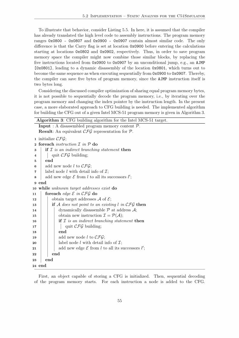
This chapter presents (theoretical) background related to formal verification and modelchecking. In what follows, the need of formal verification in the embedded systems domainis motivated by examples of famous software bugs. Next, a classification of formal verifica-tion methods is given and the term verification problem is defined. Later, the foundationsof model checking are presented and the temporal logic CTL is covered. Then, advantagesand disadvantages of model checking are discussed. Later on, the Intel MCS-51 simulatorcomponent of the [mc]square model checker is described. The chapter concludes with asummary of related work.

3.1 A World Where Nothing Works and Nobody Knows Why

Reliability is a major concern in nowadays software engineering processes. As systemcomplexity is continually rising, traditional testing methods fail to cope the verificationchallenge. Software development, even for embedded systems, has become a global taskwhere developers of various branch offices are involved. Geographically separated engineersare producing thousands or even million lines of code and perhaps have never seen eachother. Quality control of modern software production processes has become significantlydifficult [15]. On the other hand, malfunction of software is costly in terms of failure of theapplication itself but also due to the resulting consequences, such as fatal accidents, lossof money, shutting down of vital systems, reputation loss, and repayments.With this in mind, a few selected, famous software failures are presented and briefly

discussed.

Explosion of the Ariane 5 launcher on its maiden flight (1996). The maiden flight ofthe Ariane 5 launcher in June 1996 failed because of a malfunction in the controlsoftware. An untreated software trap caused the self-destruction of the rocket only37 seconds after the launch. A failed data conversion from 64 bit long floating pointto 16 bit long signed integer is arguable one of the most expensive software bugs inthe aerospace industry (cf. [16]).

Loss of the NASA Mars Climate Orbiter (1999). The spacecraft was intended to enterthe Mars orbit at an altitude of 140-150 km above the surface. The navigationsoftware failed, and caused the spacecraft to reach an altitude as low as 57 km. Thespacecraft was destroyed by atmospheric stresses and friction at this low altitude. The

5

http://www.geraldmweinberg.com/

3 Background

root cause for the loss of the spacecraft was the failure to use imperial units insteadof metric units, leading to an erroneous trajectory computed using this incorrect data(cf. [17]).

US-Northeast blackout (2003). A massive power outage on August 14th, 2003, affectedover 50 million people in northeastern USA and eastern Canada. A previously un-known software flaw in a widely-deployed energy management system contributed tothe devastating scope of the blackout. The software flaw caused alarm systems tostall because of a race condition (cf. [18]).

Toyota Prius software causes stopping and stalling on highways (2005). A softwarebug in the Electronic Control Module (ECM) causes Toyota Prius gas-electric hybridcars to stall or shut down while driving at highway speeds. Approximately 75,000vehicles were affected by this software bug (cf. [19]).

Microsoft Excel multiplication bug (2007). Any multiplication evaluating to 65,535 willdeliver incorrect results in early version of Microsoft Excel 2007. For instance, themultiplication of 850 by 77.1 results in 100,000 instead of the correct value of 65,535(cf. [20]).

A1 mobile network breakdown (2008). A software problem was responsible for thebreakdown of the mobile network service in October 2008, affecting nearly 500,000customers in Lower Austria and Vienna (cf. [21]).

ÖBB train ticketing machine selling single fare tickets for 3720.8 e (2008). A singlefare ticket for the domestic railway line between Hollabrunn (Lower Austria) andHandelskai (Vienna) is normally sold for 6.8 e. However, in some rare cases thefully automatic ticket machine at the platform charges the passenger 3720.8 e. Thathappens only in case the language is changed from German to English before theticket buying process is initiated (speaking from the author’s own experience).

Even when strictly abiding software programming rules and design guidelines, softwareis man-made and, therefore, may never be perfect. The development and use of methodsattempting to remove man-made errors in software engineering is crucial to pave the wayfor further advances in software engineering. This is the ultimate goal of formal softwareverification. Hence, the formal approach of software verification may be seen as a majorcontributor to software correctness, reliability, and safety of present and future applica-tions.

3.2 Formal Verification

Over the past decade we have learnt that software programs and hardware designs ingeneral – even after intensive testing efforts – are containing bugs (see Section 3.1). Morethan half of the development time for modern embedded designs is spent on testing anddebugging in order to approach a reliable design. While the software industry is rathersupporting the development of improved testing methods, computer scientists tend tofind alternative approaches to close the predominant verification gap in modern designs.Numerous research endeavors propose formal verification as the answer to some verificationissues. Formal verification has been one of the hot topics in computer science research for

6

3.3 The Verification Problem

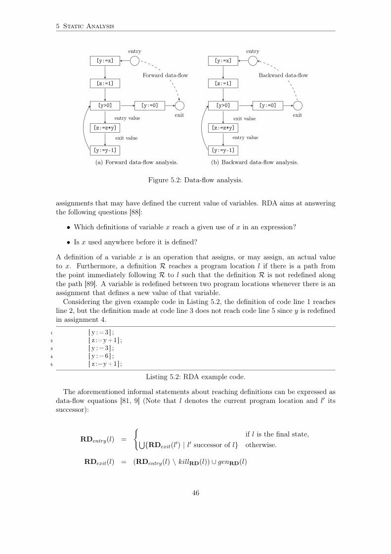
more than four decades [22]. Figure 3.1 gives a rough classification of formal verificationmethods.The main concept behind formal verification relies on the observation that computer

programs can be seen as mathematical objects with well-determined behavior. Mathemat-ical logic is used to describe the desired behavior of the computer program which is subjectto verification. The process of formally verifying a program is now to give a mathematicalproof to show that the program works as specified.

Testing &simulationFormal verification

Theoremproving

Modelchecking

Explicitmodel

checking

Symbolicmodel

checking

Figure 3.1: Formal verification methods classification.

Basically, literature distinguishes two main areas of formal software verification ap-proaches. The first one is a rather mathematical related one, called theorem proving.In theorem proving, a proof of correctness is achieved through the derivation of a theo-rem. A short overview of theorem proving is given in [23]. However, software verificationcan also be achieved without explicitly establishing mathematical proofs. The more pop-ular approach to formal verification is called model checking and is very well received inmodern-day software development processes.

3.3 The Verification Problem

The verification problem can be simply stated as [22]: Given a program M and its spec-ification ϕ determine whether or not the behavior of M meets the specification, i.e., doesM |= ϕ hold?

Alan Turing [24] formulated the problem in terms of Turing Machines. Given a TuringMachine T and a specification ϕ decide whether T will eventually halt, e.g., on a blankinput tape. That leads to the halting problem which is proven to be algorithmicallyunsolvable. Although the halting problem is unsolvable, practical formal verification provesits strength in closing the verification gap since one usually focuses on finite state systemsrather than reasoning about infinite behavior (cf. Section 4.1.2).State of the art embedded designs are reaching an unprecedented level of complexity and

7

3 Background

the observed shift from stand-alone to real ubiquitous, pervasive, and networked safety-critical applications calls for effective methods to formally prove the correct behavior of adesign. Until now, the advances in formal verification helped to successfully verify simpleprograms of moderate size that are used in safety critical applications. As recently pro-nounced by Hoare and Misra the forthcoming challenge in the field of formal verificationis seen as the process of merging the elaborated theoretical understanding of computerprograms as well as existing tools in order to enable fully automatic verification of real life,large scale, and complex embedded designs.In [25], Hoare and Misra proclaim the verification grand challenge as an international

project to construct a program verifier that would use logical proof to give an automaticcheck of the correctness of programs submitted to it. What sounds for a moment out oftouch with reality is, based on their assumptions, within the reach of the next 20 years. Intheir vision the verification grand challenge will lead to a tool that can be seen as the “swissarmy knife” of formal verification, solving the verification challenge for future hardware andsoftware designs. Hoare and Misra estimated more than a thousand person-years of effortto accomplish this project. To get an idea of the complexity of such a project: the LinuxKernel v2.6 – one of the world’s largest software projects – started its development backin 1991 and since then the development effort has gained an accumulated number of fivethousand person-years [26].The verification grand challenge is undoubted an ambitious and catchy project, never-

theless, if it succeeds it will revolutionize the way how we develop (safety-critical) softwareand it will make essential contributions to reliability, safety, and trustworthiness of futuresoftware developments. In 2002, the US Department of Commerce estimated annual coststo the US economy of about 60 billion US dollars due to avoidable software errors [27].Thus, producing error-free software is not only safe for people using those systems it iseven highly economical advantageous.It is a long and steep way to the fully automatic, formal software verification and con-

tributions made in order to achieve this ambitious goal come piece by piece. Hence, thework put into this thesis can be seen as a small step towards Hoare and Misra’s vision ofa fully automatic software verification.

3.4 Model Checking

Model checking [28, 29] is an automatic, model-based, property verification approach withthe aim to automatically verify finite state systems. The main concept behind modelchecking is basically a straightforward brute force exploration of the states of a givensystem to check whether the given system model satisfies a certain property (specification).Model checking was introduced in the early 1980’s and pioneered independently by Clarkeand Emerson [30] in the US and by Quielle and Sifakis [31] in France.Comprehensive research on (i) efficient search algorithms in order to ensure minimal

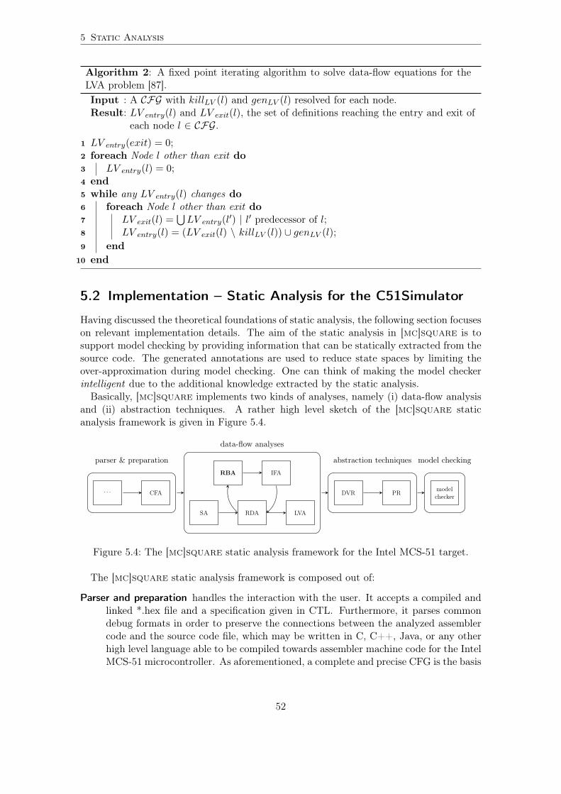
effort when traversing system states and (ii) abstraction techniques to combat the state-explosion problem was a major contributer to shift model checking from research applica-tions to industry practice. With the ever increasing available computational power it isnow possible to check systems ranging close to real life industry applications.

8

3.4 Model Checking

3.4.1 The Model Checking Problem

The model checking problem is an instance of the verification problem (cf. Section 3.3).Model checking provides an automated method for verifying concurrent (nominally) finitestate systems that uses an efficient and flexible graph search, to determine whether or notthe ongoing behavior described by a temporal property holds of the system’s state graph.The method is algorithmic and often efficient because the system is finite state, despitereasoning about infinite behavior [32].

3.4.2 The Kripke Structure

In model checking, finite (nondeterministic) state machines are used to represent the be-havior of the system. A special type of these state machines are Kripke structures. Everysingle state is labeled with Atomic Propositions (AP) which are boolean variables andthe evaluations of expressions in that state. These expressions correlate to the particularsystem properties, e.g., boolean expressions over variables or registers. A Kripke structureM is represented as an ordered sequence of four objects:

M = (S, s0,R,L)

S: finite set of statess0: initial state s0 ⊆ S

R: transition relation R ⊆ S × SL: interpretation function L :→ 2AP

The transition relation R specifies for each state whether and which successor states arepossible, i.e., for each state s ⊆ S there is a successor state s′ ⊆ S. The interpretationfunction L labels each state with the set of AP that are true in that state. A path π in theKripke structure M from a state s is a sequence of states π = s0s1s2... such that s0 = sand R(si, si+1) holds for all i ≥ 0 [28].

3.4.3 The Temporal Logic CTL

Computational Tree Logic (CTL) is a combination of a linear temporal logic and abranching-time logic and was proposed by Clarke and Emerson in 1980 [33]. The modelof time is a tree-like structure in which the future is not determined. In model checking,temporal logic is used to express the systems specification, i.e., the property ϕ. In a lineartemporal logic, various operators are provided to describe events along a single computa-tion path. In contrary, a branching-time logic provides operators to quantify over a set ofstates that are successors of a given (the current) state. CTL combines these two kindsof operators and properties are therefore constructed from path quantifiers and temporaloperators.

CTL Path Quantifiers

• A – for All paths from a certain state on

• E – there Exists at least one single path leaving from a certain state

9

3 Background

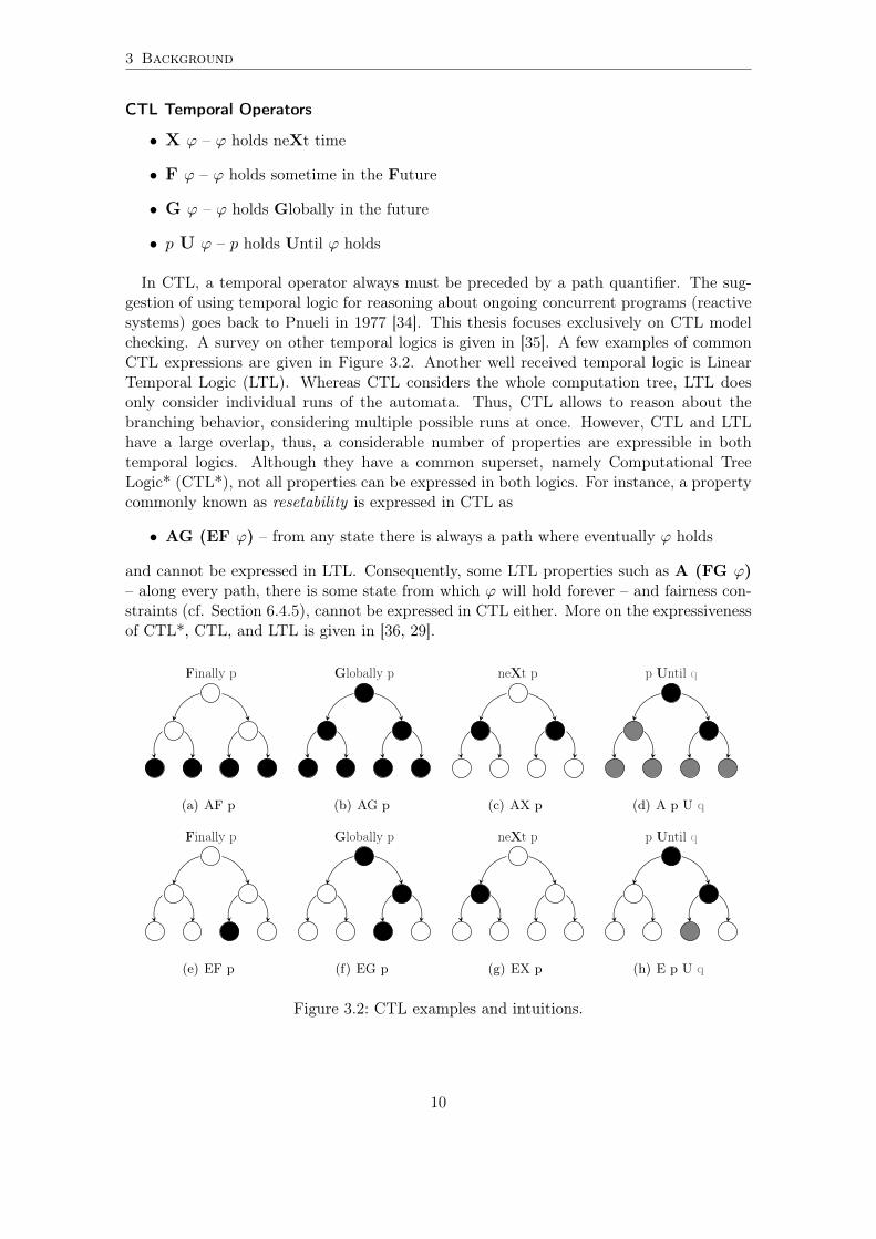
CTL Temporal Operators

• X ϕ – ϕ holds neXt time

• F ϕ – ϕ holds sometime in the Future

• G ϕ – ϕ holds Globally in the future

• p U ϕ – p holds Until ϕ holds

In CTL, a temporal operator always must be preceded by a path quantifier. The sug-gestion of using temporal logic for reasoning about ongoing concurrent programs (reactivesystems) goes back to Pnueli in 1977 [34]. This thesis focuses exclusively on CTL modelchecking. A survey on other temporal logics is given in [35]. A few examples of commonCTL expressions are given in Figure 3.2. Another well received temporal logic is LinearTemporal Logic (LTL). Whereas CTL considers the whole computation tree, LTL doesonly consider individual runs of the automata. Thus, CTL allows to reason about thebranching behavior, considering multiple possible runs at once. However, CTL and LTLhave a large overlap, thus, a considerable number of properties are expressible in bothtemporal logics. Although they have a common superset, namely Computational TreeLogic* (CTL*), not all properties can be expressed in both logics. For instance, a propertycommonly known as resetability is expressed in CTL as

• AG (EF ϕ) – from any state there is always a path where eventually ϕ holds

and cannot be expressed in LTL. Consequently, some LTL properties such as A (FG ϕ)– along every path, there is some state from which ϕ will hold forever – and fairness con-straints (cf. Section 6.4.5), cannot be expressed in CTL either. More on the expressivenessof CTL*, CTL, and LTL is given in [36, 29].

Finally p

(a) AF p

Globally p

(b) AG p

neXt p

(c) AX p

p Until q

(d) A p U q

Finally p

(e) EF p

Globally p

(f) EG p

neXt p

(g) EX p

p Until q

(h) E p U q

Figure 3.2: CTL examples and intuitions.

10

3.4 Model Checking

3.4.4 The Model Checking Workflow

In practice, the system modelM is described by a semantical model, i.e., a Kripke structureand the specification (property) ϕ is described by a formula given in temporal logic.

S1 S2

S3

(1) AG (event U abort)(2) EF event > 100(3) EF event = 20

SystemmodelM

System property ϕ

Modelchecker

M |= ϕ?

Notification Counterexampleyes no

Figure 3.3: The model checking workflow.

Proving a certain property is performed by determining the truth of formulas in certainsystem states. In order to apply model checking, one needs a modeling language in whichthe system is described as well as a notation for the formulation of properties and algorithmsto step through the state space. As shown in Figure 3.3, a typical model checking workflowis composed of three major steps:

Define a formal model of the system that is subject to verification by creating a modelof the system in a language that fits the model checker’s input language. Thosemodeling languages are usually tight coupled to the model checker itself, such asProcess or Protocol Meta Language (PROMELA) used by the SPIN model checker[37]. System modeling usually involves the process of abstraction (see Section 4.1),i.e., simplifying the original system. System modeling focuses on the main propertiesin order to better manage the system complexity.

Provide a particular system property that should be proved. In other words, a question

11

3 Background

about the system behavior is formulated that should be answered by the modelchecker. The system property is usually derived from the specification and given ina temporal logic.

Invoke the model checking tool and receive a notification whether the given systemproperty was fulfilled or not. In case the system property could not be verified,a counterexample is generated to finger-point to the source of error in the systemmodel.

3.4.5 Coffee Vending Machine Example

A simple model of a coffee vending machine is introduced to exemplify the use of Kripkestructures and CTL. Its textual specification reads as follows:

• After inserting a coin, the user can choose her/his favorite coffee.

• A coffee is only brewed after a valid selection is made.

• The user is able to abort the procedure at any time.

Figure 3.4 shows the resulting Kripke structure, with all the states, transitions, and statevariables. Each state is labeled with the atomic propositions AP that are true or false inthe state. The labels given on the transitions are not part of the Kripke structure itself.The coffee vending machine can be formally written as:

M = (S, s0,R,L)

S := S1,S2,S3s0 := S1

R := (S1,S2), (S2,S1), (S2,S3), (S3,S1), (S3,S3)L(s1) = ¬coin,¬brew,¬selectionL(s2) = coin,¬brew,¬selectionL(s3) = coin, brew, selection

As noted in Section 3.4.1, model checking is based on a graph search, therefore, thetransition system is transformed to computation paths. This is done by unwinding theKripke structure to obtain a computation tree, as shown in Figure 3.4(b).Most model checkers expect system properties given in some temporal logic. For the

coffee vending machine meaningful system properties might be:

• Coffee is brewed after a selection was made.

• Coffee is brewed sometime.

These properties can be written in CTL as:

• AG[selection⇒ brew]1 Whenever a selection is made coffee is brewed for sure.

• EF[brew] There is a state where coffee is brewed.1⇒ represents implication (first order logic).

12

3.4 Model Checking

S1start

¬coin¬brew¬selection

S2

coin¬brew¬selection

S3

coinbrew

selectioninsert coin select

abort

brewinggive change

(a) Kripke structure.

S1

S2

S3 S1

S3 S1 S2

S3 S1 S2 S3 S1

... ... ... ... ...

(b) The first computation paths.

Figure 3.4: The coffee vending machine example.

3.4.6 Local vs. Global Model Checking Algorithms

In literature, there are two different approaches of exploring the state space of a givensystem, i.e., local and global model checking algorithms. A global model checking algorithmfirst builds the whole state space. Search and labeling algorithms are applied afterwardsto find particular states in which the system property cannot be proven. In global modelchecking the state space is traversed backwards to find counterexamples. As the wholestate space is available, a global model checking algorithm is able to present all possiblecounterexamples. It may compare the length of the counterexamples and only present theshortest to the user. A major drawback of global model checking is the generation of statesthat are not relevant to prove the given formula, thus, making the state-explosion problemeven worse.Consequently, in local or on-the-fly model checking only states are visited that are needed

to prove the truth value of the formula in a given state. Hence, on-the-fly state spacebuilding is possible when using local model checking algorithms. It is obvious that a localmodel checking algorithm can hardly find the shortest counterexample. Nevertheless, localmodel checking is a first step to alleviate the state-explosion problem.

[mc]square implements a local model checking algorithm as described by Heljankoin [38]. A comparison of local and global model checking is elaborated in [39].

3.4.7 The Pros and Cons of Model Checking

Compared to traditional approaches, such as simulation and testing, model checking offerstwo major advantages:

• Model checking is a fully automatic approach. It does neither require user guidancenor does it claim for user expertise in the fields of mathematics, logic, or theoremproving. Anyone who uses design and simulation tools is able to apply model check-ing, since modern tools aim to offer a push-button solution. Model checkers areintegrated within existing design tool chains.

• Counterexample generation. Whenever the model checker reveals that a given prop-erty failed to hold, the process of model checking allows to produce a counterex-ample/witness. A counterexample finger-points the user to the root cause of theproblem, by demonstrating a behavior that falsifies the property. For the process of

13

3 Background

debugging, such an error trace is profoundly advantageous, since the counterexamplegives a complete insight into the system’s behavior.

Nevertheless, all that glitters is not gold. The broad application of model checking inindustry is taking place quite slowly, mainly because of its three major disadvantages:

• The state-explosion problem. The main challenge in model checking is to cope theproblem of state-explosion. In general, a model checker aims to enumerate and ana-lyze the set of states a system may ever reach. The overall number of system states,even when dealing with small systems, is often too large to be handled with reasonablecomputing resources. Peled [40] summarizes effective strategies for fighting againststate-explosion and proposes a combination of Binary Decision Diagrams (BDD)2,Partial Order Reduction (POR), and Symmetry. More details are also given byClarke et al. in [28].

• Reported errors may be false negatives [40]. Model checking requires, as the nameimplies, modeling of the system. In order to alleviate the state-explosion problem,abstraction is needed (cf. Section 4.1). Thus, the program that is verified may notbe the original one and consequently, if model checking reports a property violationin the abstracted model of the system, one has to make sure that the error is indeeda real one, i.e., it can be reconstructed on the real target platform. The process ofchecking the counterexample on the real system is often carried out manually. Falsenegatives arise from the differences between an actual system’s behavior and thebehavior represented by the abstracted model. Manually ruling out false negatives istime intensive and an error prone task itself. Therefore, a major future challenge forthe model checking community may be the automated elimination of false negatives.A more detailed discussion on how to overcome the problem of false negatives iscarried out in Section 7.1.

• Model checking can only verify a given specification. Thus, an important point is thecompleteness of the specification. It is challenging to make sure that the specificationcovers all properties that the system should satisfy and to establish a one to one matchof a given textual specification and the derived formal specification.

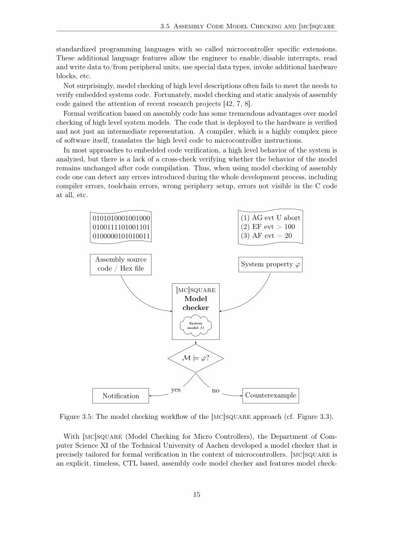
3.5 Assembly Code Model Checking and [mc]square

An important point in embedded software verification is the mismatch between what getsverified during system verification and the actual version of the application running onthe embedded target processor. In other words, there may be a mismatch between thesystem model and the actual version which is deployed in the field. As widely known anddiscussed in [41], embedded processors do not execute the high level representation of thesoftware application directly, e.g., C or C++ code, they can only execute mnemonics thatare part of the instruction set.Especially for the embedded systems domain, custom-designed microcontrollers are in

use. Most of the specific microcontroller features cannot be directly invoked throughthe high level programming language. Therefore, compiler and toolchain provider extend

2A BDD or a Propositional Directed Acyclic Graph (PDAG) is a data structure that is used to representa boolean function. It can be seen as a compressed representation of sets.

14

3.5 Assembly Code Model Checking and [mc]square

standardized programming languages with so called microcontroller specific extensions.These additional language features allow the engineer to enable/disable interrupts, readand write data to/from peripheral units, use special data types, invoke additional hardwareblocks, etc.Not surprisingly, model checking of high level descriptions often fails to meet the needs to

verify embedded systems code. Fortunately, model checking and static analysis of assemblycode gained the attention of recent research projects [42, 7, 8].Formal verification based on assembly code has some tremendous advantages over model

checking of high level system models. The code that is deployed to the hardware is verifiedand not just an intermediate representation. A compiler, which is a highly complex pieceof software itself, translates the high level code to microcontroller instructions.In most approaches to embedded code verification, a high level behavior of the system is

analyzed, but there is a lack of a cross-check verifying whether the behavior of the modelremains unchanged after code compilation. Thus, when using model checking of assemblycode one can detect any errors introduced during the whole development process, includingcompiler errors, toolchain errors, wrong periphery setup, errors not visible in the C codeat all, etc.

(1) AG evt U abort(2) EF evt > 100(3) AF evt = 20

010101000100100001001111010011010100000101010011

Assembly sourcecode / Hex file System property ϕ

[mc]squareModelchecker

Systemmodel M

M |= ϕ?


Figure 3.5: The model checking workflow of the [mc]square approach (cf. Figure 3.3).

With [mc]square (Model Checking for Micro Controllers), the Department of Com-puter Science XI of the Technical University of Aachen developed a model checker that isprecisely tailored for formal verification in the context of microcontrollers. [mc]square isan explicit, timeless, CTL based, assembly code model checker and features model check-

15

3 Background

ing and static source code analysis of software written for embedded targets. Supportedtarget platforms are the ATMEL ATMega series [9], the Intel MCS-51 [11], the InfineonXC16x [43], and Programmable Logic Controllers (PLCs) [44].The [mc]square model checker uses an accurate and customized Central Processing

Unit (CPU) simulator to automatically derive the system model out of an implementation.Thus, the manual and often error-prone process of model creation can be shifted from thetest engineer towards the implementation of the verification tool. This leads to the revisedmodel checking workflow as shown in Figure 3.5.In the following, a high level introduction to the C51Simulator component of

[mc]square is given and only those parts of the model checker are discussed that arerelevant for the elaboration of this thesis. More details on assembly code model checkingand the tool [mc]square are given by Schlich in [9].

3.6 C51Simulator – Intel MCS-51 Simulator Component

[mc]square uses a customized microcontroller simulator component for state space build-ing. Hence, in order to support new target platforms a microcontroller simulator has tobe created. The following section describes this process for the Intel MCS-51 simulatorcomponent. More details on the actual implementation can be found in [45, 11].

3.6.1 The Intel MCS-51 Microcontroller

The Intel MCS-51 success story started back in 1980, when Intel started to ship its brandnew microcontroller family, widely known as 8051, which later on became one of themost popular and successful microcontrollers ever. Nowadays, almost every well-knownIntegrated Circuit (IC) manufacturer3 has the Intel MCS-51 in its product portfolio orthey even made their own instruction set compatible derivatives.Moreover, open-source synthesizable Intel MCS-51 Intellectual Property (IP) cores are

available in Register Transfer Level (RTL) code such as Very High Speed Integrated Cir-cuit Hardware Description Language (VHDL) or Verilog, ready to be used within FieldProgrammable Gate Array (FPGA) and Application Specific Integrated Circuit (ASIC)based designs. The original Intel MCS-51 design directly influenced a remarkable numberof recent microcontroller architectures.Basically, it is an 8 bit Complex Instruction Set Computer (CISC) microcontroller orga-

nized as Harvard Architecture. Code and data memory are strictly separated and instruc-tions differ in their length.

Main Features [46, 47]:

• 128 bytes of Internal Random Access Memory (IRAM)

• 4096 bytes of internal Program Read Only Memory (ROM)

• 32 byte of bitaddressable memory block

• Four 8 bit wide general purpose I/O ports

3an estimated number of over fifty companies worldwide.

16


• Two 16 bit timer units

• Full-Duplex Universal Asynchronous Receiver Transmitter (UART)

• Five different interrupt sources and two levels of interrupt priorities

• 256 different instructions

• Five different addressing modes

• The majority of instructions are executed within 12 system clock cycles

Registers as well as I/O ports are memory mapped, therefore, accessed like any othermemory location. The stack is located within the IRAM area and grows to higher datamemory addresses. A particular and powerful architecture feature is the bit-manipulatingcapability of the CPU. Single bits can be set, cleared, or involved in other logical calcu-lations. Four separate register banks are located at the bottom of the IRAM occupyingthe first 32 bytes of data memory. Register banks are altered by modifying two dedicatedregister bank selection bits within the Program Status Word (PSW). 21 Special FunctionRegisters (SFRs) allow the configuration of peripherals. A few of them are bitaddressable,some are only byteaddressable and some can be accessed in either mode.

Instruction Set

The instruction set covers 256 different instructions, hence, resulting in 8 bit wide opcodes.Caused by the CISC architecture, instructions are either one, two, or three byte long. Theycan be separated into five groups: logical, arithmetic, program branching, data transfer,and boolean operations.

Supported Addressing Modes

Data and program memory are accessed by one of the five available addressing modes:

Immediate addressing is used whenever the source operand is a constant value ratherthan a variable. The constant value can be either included as a single byte into theinstruction, or be derived from the opcode itself.

Direct addressing is used for accessing any IRAM location including SFRs.

Indirect addressing uses the registers R0 or R1 from the active register bank as base regis-ters. The value stored into these registers indicates an address in IRAM where datashould be read from or written to. Any pointer makes use of indirect addressing.

Extended direct addressing is basically the same as direct addressing but it is rather usedto access additional external memory locations than IRAM locations.

Indirect from program memory enables reading from program memory.

The interested reader is referred to the Intel MCS-51 datasheet [46] for more details onthe architecture and the instruction core.

17

3 Background

3.6.2 The Big Picture

[mc]square uses a well defined and slim interface to communicate and control theC51Simulator. The main task of the C51Simulator is to generate possible successor statesfor a given Program Counter (PC) location. In order to do so, the C51Simulator hasto model and implement the whole instruction set, data memory management as well asperipheral units of the real target microcontroller. However, a few requirements (cf. [11])for the simulator forbid the use of existing CPU simulators. [mc]square abstracts fromtime, hence, the use of an existing and off-the shelf CPU simulator is not suitable for the[mc]square approach to assembly code model checking. Almost all Commercial Off TheShelf (COTS) microcontroller simulator engines are based on a cycle accurate approach.Thus, without applying further modifications it is nearly infeasible to use conventionalcycle-accurate simulator engines to build [mc]square conform state spaces. Moreover,some abstraction techniques are applied on-the-fly, i.e., during the state space generation,requiring extra behavior not found in standard CPU simulators.

binary &debugfiles

programparser

CTLproperty

CTLparser

staticanalyzer

statespace

simulators

c167C51

. . .

AVRPLC

counter-examplegen.

Figure 3.6: The [mc]square framework.

As shown in Figure 3.6 the [mc]square framework provides a full CTL model checker,a counterexample generator, a comfortable Graphical User Interface (GUI), and an assem-bly code static analyzer. Whenever [mc]square needs data generated by the hardwarethe respective simulator component is invoked. A nice side effect of the simulator basedapproach is a full CPU simulator, allowing the user to analyze and debug the code priorto model checking. It is notable that [mc]square offers a new way of analyzing micro-controller programs, which is quite different to standard COTS tools, since the simulationcovers the whole state space of the application.

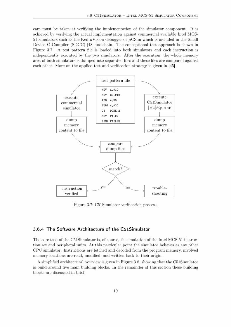
3.6.3 Test and Verification of the C51Simulator Component

Amajor point of criticism on tool based model checking, is the justifiable question regardingthe verification of the tool itself. How to make sure that the tool doesn’t contain softwarebugs by itself, leading to false outputs during the model checking process? Hence, special

18


care must be taken at verifying the implementation of the simulator component. It isachieved by verifying the actual implementation against commercial available Intel MCS-51 simulators such as the Keil µVision debugger or µCSim which is included in the SmallDevice C Compiler (SDCC) [48] toolchain. The conceptional test approach is shown inFigure 3.7. A test pattern file is loaded into both simulators and each instruction isindependently executed by the two simulators. After the execution, the whole memoryarea of both simulators is dumped into separated files and these files are compared againsteach other. More on the applied test and verification strategy is given in [45].

MOV PSW,#0

MOV A,#10

MOV R0,#10

ADD A,R0

SUBB A,#20

JZ DONE_2

MOV P1,#2

LJMP FAILED

test pattern file

executecommercialsimulator

executeC51Simulator[mc]square

dumpmemory

content to file

dumpmemory

content to file

comparedump files

match?

instructionverified

trouble-shooting

yes no

Figure 3.7: C51Simulator verification process.

3.6.4 The Software Architecture of the C51Simulator

The core task of the C51Simulator is, of course, the emulation of the Intel MCS-51 instruc-tion set and peripheral units. At this particular point the simulator behaves as any otherCPU simulator. Instructions are fetched and decoded from the program memory, involvedmemory locations are read, modified, and written back to their origin.A simplified architectural overview is given in Figure 3.8, showing that the C51Simulator

is build around five main building blocks. In the remainder of this section these buildingblocks are discussed in brief.

19

3 Background

DeterminizerSplitterMemorymodel

Instructionset core

Interface

[mc]square

Figure 3.8: Software architecture of the C51Simulator.

Instruction Set Core

A basic, straightforward implementation of the semantics of the opcodes supported by themicrocontroller as defined in the corresponding datasheet [46].

Memory Model

The memory model acts as a representation of the Intel MCS-51 data and program memory.As described in [49], [mc]square uses abstraction techniques that center around the ideaof a 3-valued memory representation. Such a ternary memory representation allows certainmemory locations to be marked as unknown in order to avoid the creation of unneededsuccessor paths. For this reason, the memory model requires shadow memory to indicatewhether the actual value is known.Consequently, the simulator manages two blocks of memory. As shown in Table 3.1,

every byte of memory is represented by its actual value and a second byte, serving asmask indicating whether or not a certain bit is deterministic (Those bits with valueNondeterministic (ND) are indicated by a *).

Location Binary value ND-mask Ternary value@ 0x0A b 11110000 b 00001100 1111**00@ 0x0B b 00001111 b 11110000 ****1111@ 0x0C b 10101010 b 01010101 1*1*1*1*@ 0x0D b 00000000 b 01100110 0**00**0@ 0x0E b 00110011 b 00000000 00110011@ 0x0F b 01010101 b 11111111 ********

Table 3.1: Memory representation in [mc]square.

More on the benefits of this 3-valued memory representation is given in [13, 9] and inSection 4.1.3.

20

3.7 Related Work

Splitter

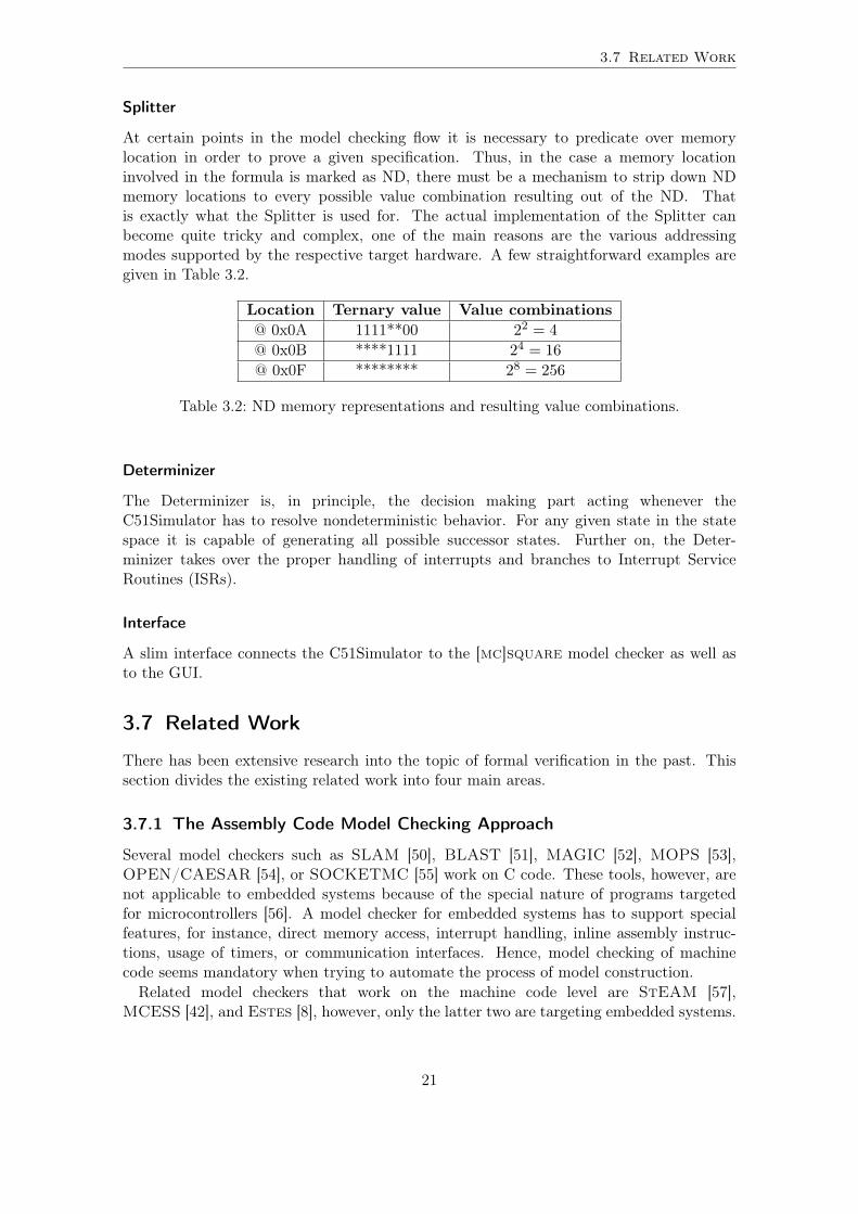
At certain points in the model checking flow it is necessary to predicate over memorylocation in order to prove a given specification. Thus, in the case a memory locationinvolved in the formula is marked as ND, there must be a mechanism to strip down NDmemory locations to every possible value combination resulting out of the ND. Thatis exactly what the Splitter is used for. The actual implementation of the Splitter canbecome quite tricky and complex, one of the main reasons are the various addressingmodes supported by the respective target hardware. A few straightforward examples aregiven in Table 3.2.

Location Ternary value Value combinations@ 0x0A 1111**00 22 = 4@ 0x0B ****1111 24 = 16@ 0x0F ******** 28 = 256

Table 3.2: ND memory representations and resulting value combinations.

Determinizer

The Determinizer is, in principle, the decision making part acting whenever theC51Simulator has to resolve nondeterministic behavior. For any given state in the statespace it is capable of generating all possible successor states. Further on, the Deter-minizer takes over the proper handling of interrupts and branches to Interrupt ServiceRoutines (ISRs).

Interface

A slim interface connects the C51Simulator to the [mc]square model checker as well asto the GUI.

3.7 Related Work

There has been extensive research into the topic of formal verification in the past. Thissection divides the existing related work into four main areas.

3.7.1 The Assembly Code Model Checking Approach

Several model checkers such as SLAM [50], BLAST [51], MAGIC [52], MOPS [53],OPEN/CAESAR [54], or SOCKETMC [55] work on C code. These tools, however, arenot applicable to embedded systems because of the special nature of programs targetedfor microcontrollers [56]. A model checker for embedded systems has to support specialfeatures, for instance, direct memory access, interrupt handling, inline assembly instruc-tions, usage of timers, or communication interfaces. Hence, model checking of machinecode seems mandatory when trying to automate the process of model construction.Related model checkers that work on the machine code level are StEAM [57],

MCESS [42], and Estes [8], however, only the latter two are targeting embedded systems.

21

3 Background

Estes model checks assembly code for the 68HC11 microcontroller constructing the statespace either with a simulator or real hardware using the GNU debugger. In practice, thisapproach is only feasible for small programs. Constructing the state space for the model viathe hardware takes time (unless dedicated hardware support is provided). Furthermore,using an out-of-the-box simulator/debugger to construct the model, on the other hand,restricts optimizations in order to minimize the state space. MCESS, in contrast, trans-lates the assembly code of ATMEL ATmega 16 microcontrollers into hardware-independentbyte-code for a specific virtual machine that is able to check properties given in LTL. How-ever, due to this approach most hardware issues are abstracted rather coarse eventuallyremoving essential information that may invalidate the entire verification process.Unlike these approaches, [mc]square constructs the model with special, tailored simu-

lators for microcontrollers.

3.7.2 3-valued Abstraction Techniques

3-valued logic was initially defined by Kleene [58]. 3-valued logic is used in many researchareas connected with verification. There are model checking algorithms that directly workwith 3-valued logic. Bruns and Godefroid [59] describe a 3-valued CTL model checkingalgorithm. Another approach is described in a paper written by Yahav [60]. In this paper,3-valued logic is used to verify safety properties of concurrent Java programs. In contrastto these approaches, the model checking algorithms used by the [mc]square approachwork with Boolean logic. 3-valued logic is only utilized in the memory representation thatis used by the simulator, which builds the state space. All memory locations that areaccessed by the model checking algorithms use Boolean logic.Symbolic or X-valued simulation [61] is another technique that is related to 3-valued

logic. Here, symbolic values are used in place of explicit values. In our approach partsof the states used can be symbolic, but whenever the simulator or the model checkerneeds to access symbolic parts of a state, these parts are instantiated, and hence becomeexplicit. All parts of a state that are not accessed remain symbolic. In [62] a symbolicsimulation scheme is used to verify embedded array systems such as memory managementunits of high performance microcontrollers. Symbolic Trajectory Evaluation (STE) [63]is a lattice-based model checking technology that uses a form of symbolic simulation forhardware circuit verification.In [61], a symbolic simulator is used to verify hardware systems. Similar [64] combines

a linear-time logic model checking algorithm with lightweight theorem proving in higher-order logic. Whenever an X (denoted by ND in our approach) is accessed and a valueis needed, new symbolic variables are added and simulation has to be repeated. In ourmethod a dynamic refinement is conducted. There are some approaches combining explicitand symbolic executions (cf. [65, 66]), but these approaches do explicit execution andsymbolic execution in parallel.There are also some approaches using 3-valued logic in static analysis. Reps et al. [67]

describe an approach to use 3-valued logic in abstract interpretation. In another paper,Sagiv et al. [68] present a way to use 3-valued logic for shape analysis. Both analyses arespecial purpose analyses. In our approach, we use the 3-valued logic in a memory modelutilized within model checking, which is a dynamic analysis that is more general.

22

3.7 Related Work

3.7.3 Static Analysis

Typical static analyzers for C are not capable of dealing with features specific to embeddedhardware due to the lack of a precise hardware model. This can be integrated though, asdescribed by Fehnker et al. [69]. In their work, a static analyzer for C/C++ code calledGoanna was extended to detect misuse of hardware features of the ATMEL ATmega16.Regehr and Reid [70] describe a system specifically suited for embedded software, which

automatically generates abstractions using the specification of the microcontroller. Anapproach to automatic generation of transfer functions for data-flow analyses is describedby Regehr and Duongsaa [71]. Their approach is to automatically derive abstractionsand transfer functions from a specification, while our approach involves modeling suchabstractions by hand. An earlier approach by Bergeron et al. [72] transforms the assemblycode into a higher-level representation, on which static analysis is performed, but they donot consider interrupts, which makes this approach unsuitable for interrupt-driven soft-ware frequently found in embedded systems. Brylow et al. [73] describe static analysisfor interrupt-driven software, but their approach supports only immediate values writteninto status registers. In practice, values written into status register are often stored andmanipulated in registers.Martin et al. [74] have described a loop analysis algorithm for cache prediction. In this

approach, loop bodies are transformed into separate functions and interprocedural anal-ysis algorithms are applied to perform a precise analysis of loops, which is similar to acontext-sensitive analysis. A stack analysis using a context-sensitive abstract interpreta-tion is described by Regehr et al. [75]. This analysis is used for a worst-case predictionof stack sizes. While interrupts are considered, recursion is unrolled only until a fixedbound specified by the user. A thorough description of challenges during static analysisof microcontroller assembly code is included. Another approach to stack analysis of x86assembly programs is described by Linn et al. [76], which is not suitable in presence ofinterrupts. An intraprocedural static slicing algorithm for assembly code is described byCifuentes and Fraboulet [77], but stack variables are not supported at all.The occurrence of interrupts in embedded software can be seen as a restricted form of

multi-threading. Numerous approaches for static analysis of concurrent programs havebeen developed. An approach by Lal and Reps [78] adapts static analyses for sequentialprograms and extends them to work in a concurrent setting. Other approaches, such asthe work by Qadeer and Rehof [79] or Lal et al. [80], tackle state-explosion due to threadinterleavings by imposing an upper bound on the number of context switches.In contrast, our approach of Register Bank Analysis aims at refining assembly code static

analysis for the Intel MCS-51 microcontroller by proposing a tailored analysis to cope withthe architectural feature of register bank swapping.

3.7.4 Simulators for [mc]square

Other simulators for [mc]square were previously implemented by Schlich [9] (ATMegafamily), Scheuer [43] (Infineon Xc167), and Wernerus [44] (PLC).

23

3 Background

24

4 Abstraction Techniques

All the world is an abstractinterpretation (of all the world).

(David Schmidt)

In this chapter the concept of abstraction is introduced and the need of abstrac-tion in model checking is emphasized. First, the terms over-approximation and under-approximation are explained. Next, a thought experiment is conducted, showing the ex-ponential connection between the state space size and the amount of data memory of amicrocontroller. Then, nondeterministic behavior in assembly code model checking is ad-dressed and a 3-valued memory model is presented. Finally, three state space abstractiontechniques and their actual implementation into the Intel MCS-51 simulator componentare described.

4.1 Abstraction in Model Checking

Abstraction refers to the progress of obtaining a simpler version of the checked system, byreducing the number of details that need to be taken care of. Abstraction is performed inorder to retain only information that is relevant for a particular purpose.

4.1.1 Reducing System Complexity through Abstraction

Abstraction is quite natural and human, e.g., the human ear is able to recognize frequenciesin a narrow bandwidth only. The bandwidth typically stretches from about 16 Hz up to20 kHz. Thus, all other frequencies are neglected, or in other words abstracted, sincethey are out of the relevant range. Ever since the early beginnings of model checkingin the late 1970’s research teams [32] are facing a problem generally known as the state-explosion problem, describing the limitation set by available computation power and theresulting states that can be stored, examined, and verified against the user-stated claims.Abstraction or simplification of the analyzed model towards manageable versions of theanalyzed system is crucial for the application of formal methods and a key concept tomitigate the state-explosion problem. Nevertheless, abstraction introduces new verificationchallenges among the original system and the simplified one [40]:

• Proving that the essential properties are preserved between the original system andits simpler version (Bisimulation relation1).

• Proving the correctness of the simplified version. This task may be achievable afterthe simplification through model checking.

1Bisimulation refers to a relation between state transition systems, associating systems which behave inthe same way in the sense that one system simulates the other and vice-versa.

25

http://people.cis.ksu.edu/~schmidt/


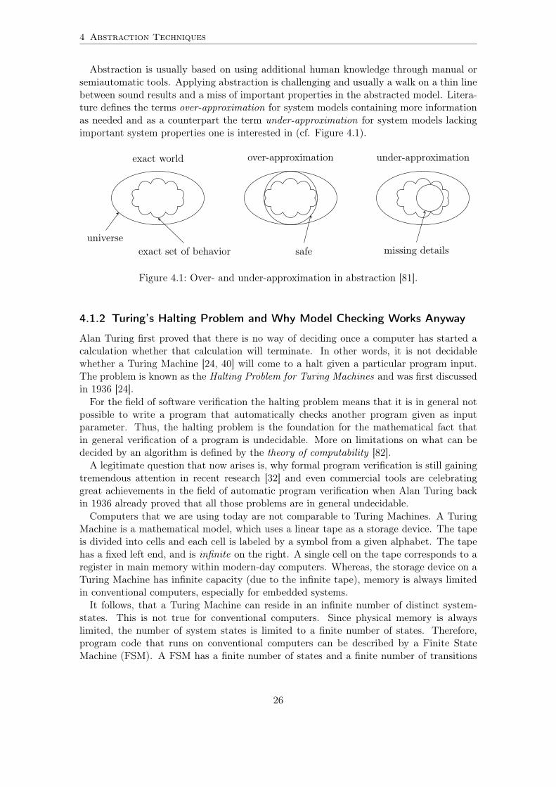
Abstraction is usually based on using additional human knowledge through manual orsemiautomatic tools. Applying abstraction is challenging and usually a walk on a thin linebetween sound results and a miss of important properties in the abstracted model. Litera-ture defines the terms over-approximation for system models containing more informationas needed and as a counterpart the term under-approximation for system models lackingimportant system properties one is interested in (cf. Figure 4.1).

exact world

universeexact set of behavior

over-approximation

safe

under-approximation

missing details

Figure 4.1: Over- and under-approximation in abstraction [81].

4.1.2 Turing’s Halting Problem and Why Model Checking Works Anyway

Alan Turing first proved that there is no way of deciding once a computer has started acalculation whether that calculation will terminate. In other words, it is not decidablewhether a Turing Machine [24, 40] will come to a halt given a particular program input.The problem is known as the Halting Problem for Turing Machines and was first discussedin 1936 [24].For the field of software verification the halting problem means that it is in general not

possible to write a program that automatically checks another program given as inputparameter. Thus, the halting problem is the foundation for the mathematical fact thatin general verification of a program is undecidable. More on limitations on what can bedecided by an algorithm is defined by the theory of computability [82].

A legitimate question that now arises is, why formal program verification is still gainingtremendous attention in recent research [32] and even commercial tools are celebratinggreat achievements in the field of automatic program verification when Alan Turing backin 1936 already proved that all those problems are in general undecidable.Computers that we are using today are not comparable to Turing Machines. A Turing

Machine is a mathematical model, which uses a linear tape as a storage device. The tapeis divided into cells and each cell is labeled by a symbol from a given alphabet. The tapehas a fixed left end, and is infinite on the right. A single cell on the tape corresponds to aregister in main memory within modern-day computers. Whereas, the storage device on aTuring Machine has infinite capacity (due to the infinite tape), memory is always limitedin conventional computers, especially for embedded systems.It follows, that a Turing Machine can reside in an infinite number of distinct system-

states. This is not true for conventional computers. Since physical memory is alwayslimited, the number of system states is limited to a finite number of states. Therefore,program code that runs on conventional computers can be described by a Finite StateMachine (FSM). A FSM has a finite number of states and a finite number of transitions

26


between those states. The upper limit of possible states is defined by all possible registerand memory configurations. The transitions are depending on the underlying hardwarearchitecture. It is even possible to generate a finite state graph for all possible programsthat may run on the computer. Each program would have a different entry node in thestate graph. Depending on the current instruction of the program – that represents thetransitions – it is possible to follow the graph in order to observe the intended behaviorby the program. As one can imagine, those (complete) state graphs are huge, even thoughtheir generation is theoretically possible.Summarized, the undecidable Halting Problem for Turing Machines is reduced for real

life computer systems with limited memory to a decidable one since the focus lies on:

• model checking of finite state machines, i.e., finite state reactive systems

• propositional temporal logics to describe properties of the FSM model

Nevertheless, model checking of assembly code remains a tough job, mainly caused by thestate-explosion problem. To illustrate the state-explosion problem, a thought experimentis conducted. Imagine an ordinary microcontroller, featuring a read-only program memoryand a read-write data memory. Each memory location is 8 bit wide. Table 4.1 shows therelation between the number of data memory bytes and the resulting states the systemmay reside in. It is evident that resulting state space is exponential in the number of thedata memory size.

Data memory size Resulting system states (state space size)1 byte 2561 = 2562 byte 2562 = 655363 byte 2563 = 167772164 byte 2564 = 42949672965 byte 2565 = 10995116277766 byte 2566 = 2814749767106567 byte 2567 = 720575940379279368 byte 2568 = 1844674407370955161616 byte 25616 = 340282366920938463463374607431768211456

Table 4.1: Data memory size and resulting system states.

In fact, for the Intel MCS-51 target, the IRAM is compiled out of 256 bytes of memory,leading to an approximate of 256256 possible system configurations2. Under the spell ofMoore’s Law – the number of transistors that can be placed inexpensively on an integratedcircuit doubles every two years [83] – the number of possible system configurations increasestremendously with every new microcontroller family.As the presented examples make clear, even for tiny systems with only a few bytes of

memory the number of possible system states is tremendous, thus, claiming the use ofabstraction in order to alleviate the state-explosion problem.

2256256 equals to a number with 616 decimal places.

27


4.1.3 Nondeterministic Behavior in Assembly Code Model Checking

One of the biggest challenges in explicit (in our case assembly code) model checking isdealing with nondeterministic behavior. Nondeterminism is introduced by the environmentin which the microcontroller is operating in, e.g., by unknown values of I/O ports. Thisuncertainty requires a dedicated treatment by the model checker. It leads to the creationof multiple successor states by instantiation of nondeterministic values with every possiblevalue combination, which in turn means a further expansion of the overall state space.Recapitulating the working scheme of [mc]square, a model of the particular micro-

controller is responsible for state space building. In general, the microcontroller softwaremodel faces nondeterminism by either performing communication with the external envi-ronment, e.g., reading a value over the I/O lines, undertaking serial communication, orby interrupts that are likely to occur at every system state as long as the correspondinginterrupt source is enabled. For the Intel MCS-51 target sources of nondeterminism are:

(i) The four I/O ports

(ii) The four timer registers

(iii) The serial communication receive register

(iv) The five interrupt flags

• Serial interrupt flag

• Timer 0/1 overflow flag

• External event 0/1 flag

To make the issue of introducing nondeterministic values clear, the assembly code snippetin Listing 4.1 is investigated. This assembly code instructs the microcontroller to read asingle byte from the 8 bit wide I/O ports P0 and P1 and stores the fetched values withinthe internal Random Access Memory (RAM) at locations 0x20 and 0x21, respectively.

1 MOV 0x20 , P02 MOV 0x21 , P1

Listing 4.1: Assembly code excerpt.

Following the idea of explicit state space generation reveals that the two assembler in-structions shown in Listing 4.1 generate altogether 256×256 = 65536 successor states. Theconsiderable number of successors is originated by the immediate instantiation of nonde-terministic values contained in I/O ports. The two MOV instructions are stored successivelyin the program memory. The value of P0 is unknown, and therefore, the model checkercreates 256 successor states to remove uncertainty concerning the actual value of the port.Afterwards, the second MOV instruction is executed. Each of the 256 successors then cre-ates further 256 successors for the instantiation of P1, whose actual value is unknown too.Environment information is not present, hence, all 65536 successors are created in order tocover all conceivable situations. Let us consider the fact of immediate successor creationfrom a different point of view. Suppose, that the stated claim that is subject to verificationdoes not include statements over memory location 0x20 nor over 0x21. In this case, thereis no need to create successors states. It is sufficient to find a mechanism to mark certainbit positions whose value is unknown and, thus, can be read as ND.

28


To that end, a 3-valued logic approach for modeling the microcontroller memory is used.Whereas binary logic is composed out of elements that are valued on the set 0, 1, i.e.,each value obtains either true or false, 3-valued logic or ternary logic [58] is defined asfollows in [84]: Ternary logic is a system ∆ whose elements called statements are valuedin the set 0, 1, 2. If x is a statement3, the value of x can be interpreted as a mappingν : ∆→ 0, 1, 2 such that:

ν(x) :=

0; if x is perhaps true, perhaps false1; if x is true2; if x is false

(4.1)

In the remainder of this thesis the term ND is used for the first line of the semanticrepresentation stated in Equation 4.1.3. Ternary logic is well known in hardware descriptionlanguages such as VHDL or Verilog to represent unknown values of, e.g., input circuitlatches or uninitialized memory locations. Synthesis tools use this ND representation toreveal design errors, which the designer can correct before synthesis towards an actualcircuit.From the state space view, the 3-valued memory representation introduces a certain type

of states, namely lazy states. A lazy state combines both explicit and symbolic parts ofthe state space4. Any state including memory locations marked as ND is called lazy state.Consequently, a single lazy state represents a set of explicit states. A lazy state and thecorresponding nondeterministic state space representation are shown in Figure 4.2.

S(n)

S(n+1)

S(n+2)

S1

lazystateS2

S3 S4

S5 S6

.. .. . .

. . . . . . . . .

set of explicit states

Figure 4.2: Nondeterministic state space representation.

3Note that in our approach a statement refers to a single bit location within the IRAM of the microcon-troller.

4[mc]square still uses explicit model checking algorithms.

29


4.2 Implementation – Abstraction Techniques for theC51Simulator

As aforementioned, abstraction is the main concept to overcome the state-explosion prob-lem. In what follows, the implemented abstraction techniques for the C51Simulator arepresented. The different concepts have different effects on the achievable state space reduc-tions as well as on the maintained expressiveness. The stronger the applied abstraction,the higher the over-approximation. The actual results strongly depend on the source codestructure, the number of I/O accesses, the number of used interrupts, etc. A rough esti-mation, based on empirical knowledge, about the effects of the three introduced conceptsare given in Table 4.2.

Abstraction State space Maintainedtechnique reduction expressiveness

none none fullDelayed Nondeterminism low high

Delayed Nondeterminism with Look Ahead medium mediumNondeterministic Program Status Word high low

Table 4.2: Comparison of abstraction techniques for the C51Simulator.

4.2.1 Delayed Nondeterminism

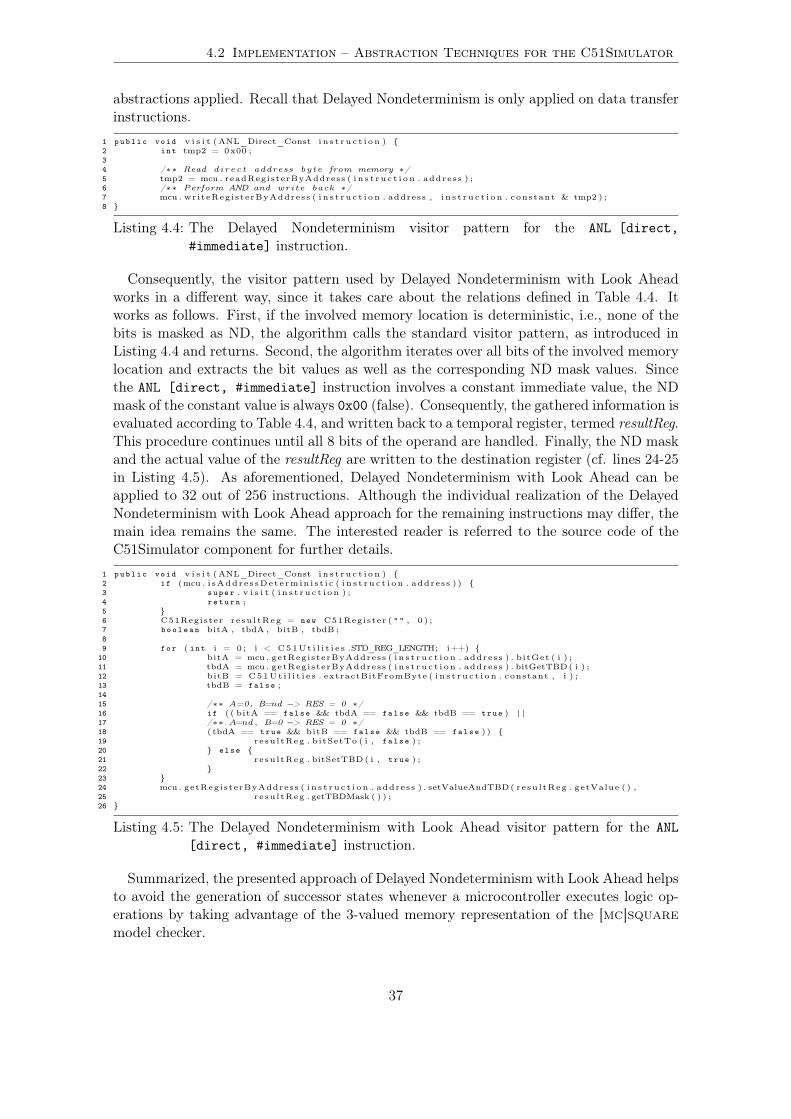
Delayed Nondeterminism was first presented in [49] and is an approach to state spacereduction. As the name implies, resolving nondeterministic values by the Splitter (cf. Sec-tion 3.6.4) is postponed as long as possible. For that reason, [mc]square takes advantageof its 3-valued memory concept. Successor states are not necessarily produced when theyare generated but only in case they are needed to prove a given system property or for asubsequent computation step. For example, a subsequent computation step is any condi-tional branch instruction, which requires the actual value of a nondeterministic memorylocation to solve the jump condition or to determine the target location where the branchleads to.

Location Binary value ND-mask Ternary valuebefore executing MOV [0xA, 0xB]

@ 0xA b 11110000 b 00000001 1111000*@ 0xB b 00001111 b 11110000 ****1111

after executing MOV [0xA, 0xB]@ 0xA b 00001111 b 11110000 ****1111@ 0xB b 00001111 b 11110000 ****1111

Table 4.3: Memory contents before and after the MOV instruction.

To illustrate the concept of Delayed Nondeterminism, the instruction MOV [0xA, 0xB]is considered. With regard to the Delayed Nondeterminism approach, whenever theC51Simulator executes a MOV instruction, not only the value from 0xB is copied to 0xA– as one would expect when reading the defined instruction semantics in the datasheet –

30

4.2 Implementation – Abstraction Techniques for the C51Simulator

it rather copies the corresponding ND-mask and the actual value. Hence, the generationof multiple successors is avoided by delaying the instantiation of the involved and perhapsnondeterministic memory location 0xB. This procedure is documented in Table 4.3 andillustrated in Figure 4.3.

Source0x0A

ND-mask

value

Destination0x0B

ND-mask

value

copy

copy

Figure 4.3: The Delayed Nondeterminism approach of handling the MOV [0xA, 0xB]instruction.

A case study by Noll and Schlich [49] revealed the effect of Delayed Nondeterminismfor different program configurations showing a possible state space reduction of 70% andabove. Nevertheless, actual savings due to Delayed Nondeterminism depend on variousfactors, such as source code structure and the targeted hardware.

4.2.2 Delayed Nondeterminism with Look Ahead

Delayed Nondeterminism with Look Ahead carries the thought of Delayed Nondeterminisma bit further. First results were presented to the scientific community in [13].Even though modern microcontrollers come along with a lot of different functionality,

there is one thing they have all in common. A typical instruction set offers at least fourdifferent kinds of operations:

1. Arithmetic operations are used whenever the microcontroller has to perform arith-metic calculations such as ADD, SUBB, INC, DEC, MUL, DIV, etc.

2. Logical operations are used whenever the microcontroller has to evaluate booleanequations. Typical examples are ANL, ORL, XRL, CPL, RLC, RRC, etc.

3. Data transfer operations are utilized whenever data/program memory is copied froma given location, i.e., the source, to a destination location. Those operations arecommonly referred to as MOV instructions.

4. Program branching operations are utilized whenever conditional or unconditionalbranches are needed in order to change the flow of execution when stepping throughthe microcontroller program. Program branching leads to a modification of the PC,thus, allowing subroutines, loops, and branches in general. Typical representativesare SJMP, LCALL, JZ, CJNE, DJNZ, etc.

Whereas Delayed Nondeterminism is only applicable for data transfer operations (3),the approach of Delayed Nondeterminism with Look Ahead focuses on logical operations(2), while still preserving all the advantages generated by Delayed Nondeterminism. Thus,

31


Delayed Nondeterminism with Look Ahead can be seen as an extension of Delayed Non-determinism. Delayed Nondeterminism fails to prove its superiority when dealing withlogic operations, since the straightforward approach of copying ND-masks, as described inSection 4.2.1, cannot be applied anymore.The main idea of the Delayed Nondeterminism with Look Ahead approach to state space

reduction is to take the semantic relations of the instructions into account. Delayed Non-determinism with Look Ahead centers around the coherence among the boolean operators∧, ∨, and ¬ with particular regard to 3-valued logic. Relevant relations are summarizedin Table 4.4

A B A ∨ B A ∧ B ¬ Atrue true true true

falsetrue ND true NDtrue false true falsefalse true true false

truefalse ND ND falsefalse false false falseND true true ND

NDND ND ND NDND false ND false

Table 4.4: Truth table for 3-valued logic.

Embedded systems code is tightly coupled to the environment of the microcontroller.Analog and digital values are read from sensors, giving the application the possibility toreact upon changes in the environment. Therefore, reading data over I/O ports of themicrocontroller is essential for embedded applications. Since reading unknown values fromthe environment is one of the major contributers to the state-explosion problem, specialcare has to be taken to avoid the generation of needless successor states from the verybeginning. Delayed Nondeterminism with Look Ahead tackles the problem right from thepoint where data is read from the I/O ports.Reading values over the microcontroller I/O often involves bitwise operations performed

by bit masks, since ports can be either accessed byte wise only, or the application is onlyinterested in a certain number of bits, e.g., the lower nibble of an 8 bit wide port. Bitmasking, or bit twiddling is a common way to individual operations on single bits. Asummary of the most common usages of bitmasks is given in Table 4.5.Compilers translate those bit-twiddling statements from the high level language towards

logic operations supported by the microcontroller’s instruction set. In the following, asimple example is presented to explain the idea of Delayed Nondeterminism with LookAhead.

Example

The C code in Listing 4.2 represents typical (low level) embedded code.In what follows, this code excerpt is used to discuss the concept of Delayed Nondeter-

minism with Look Ahead. The code reads the value of the 8 bit wide I/O port, termedPort1, and uses a bitmask to extract the upper two bits out of the I/O port.

32


Operation C code syntax Operand Mask Op Example

Setting bits to 0 y &= ~(1 « pos); 01101110 11110111 ∧011011101111011101100110

Setting bits to 1 y |= (1 « pos); 10010101 00001000 ∨100101010000100010011101

Toggling a bit y ^= (1 « pos); 10011101 00001000 ⊕100111010000100010010101

Testing a bit y = x & (1 « pos); 00011101 00001000 ∧000111010000100000001000

Extract low nibble y = x & 0x0F; 10011101 00001111 ∧100111010000111100001101

Extract high nibble y = x & 0xF0; 10011101 11110000 ∧100111011111000010010000

Table 4.5: How bitmasks are used in embedded software.

1 unsigned char readValueFromIO ( void ) 2 /∗ read por t va lue ∗/3 value = Port1 ;4 /∗∗ mask the upper two b i t s ∗/5 value &= 0xC0 ;6 return value ;7 8

9 int main ( void ) 10 while (1 ) 11 readValueFromIO ( ) ;12 /∗∗ do something ∗/13 14

Listing 4.2: Embedded C code example program for the Intel MCS-51 target.

The source code line 5 in Listing 4.2 is now mapped by the compiler (Keil C51 CompilerV8.01) to the opcode #0x53 representing the instruction ANL direct,#immediate. The ANLinstruction compares the bits of the internal memory location (0x12) with the immediatevalue (#0xC0) and sets the corresponding bit in the resulting byte only if the particular bitis set in both of the operands, otherwise the resulting bits are cleared.

1 MOV value (0 x12 ) , Port1 (0 x90 )2 ANL value (0 x12 ) , #0xC0

Listing 4.3: Translated assembly code for source code lines 4-5 of Listing 4.2.

33


In the following, the effect of the assembly code in Listing 4.3 on the abstraction tech-niques Delayed Nondeterminism and Delayed Nondeterminism with Look Ahead are dis-cussed and compared.Delayed Nondeterminism helps to avoid generating successor states for the initial MOV

instruction by simply copying the actual value as well as the ND-mask from memory loca-tion 0x90 to memory location 0x12 (cf. Figure 4.3). Reading from the environment leadsalways to a full-nondeterministic read, since environment information is not present. How-ever, Delayed Nondeterminism forces us to determinize (creating all possible successors)involved memory locations in preparation for the following ANL instruction. The variablevalue is unknown, thus, all 8 bits are marked as ND and the model checker invokes thesimulator to generate all possible successors arising from this uncertainty. The number ofsuccessor states is easily calculated and results in 28 = 256 states. Consequently, DelayedNondeterminism leads to a wide branch in the computation tree, having a negative impacton the state space and makes the state-explosion problem even worse. This scenario isdepicted in Figure 4.4, showing the total number of 256 successor states generated.

S(n)

S(n+1)

S1

S3-253

S2

value:=0x02

b00000010

S1

value:=0x01

b00000001

S0

value:=0x00

b00000000

S253

value:=0xFD

b11111101

S254

value:=0xFE

b11111110

S255

value:=0xFF

b11111111

Figure 4.4: The state-explosion problem.

However, the described approach results in a valid over-approximation (cf. Section 4.1.1)by replacing the ND value of memory location value with actual values (one at a time) andperforming the ANL afterwards. Nevertheless, this approach lacks a consideration of thesecond operand included in the operation, i.e., the constant value of the bitmask. As shownin the example code, the bitmask is of value 0xC0. Examining the bitmask on the binarylevel, it evaluates to b 11000000. Thus, the only two bits of interest in this calculationare the upper two, i.e., the two most significant bits. The remaining six bits, will evaluate,according to the relations defined in Table 4.4, to false in any case.Hence, the number of successor states can be reduced from 28 = 256 down to 22 = 4. The

resulting values are 0x00, 0x40, 0x80, and 0xC0 as detailed in Table 4.6. Figure 4.5 presentsthe differences in the number of the resulting system states for the various abstractiontechniques when executing the two assembler instructions of Listing 4.3.The Delayed Nondeterminism with Look Ahead approach helps to avoid over-

approximation whenever logical operations are performed over ND memory locations. How-

34


Bit Value Operation Mask Result CombinationsMSB *

∧

1 * (i) 0x00 ≡ b 000000006 * 1 *5 * 0 0 (ii) 0x40 ≡ b 010000004 * 0 03 * 0 0 (iii) 0x80 ≡ b 100000002 * 0 01 * 0 0 (iv) 0xC0 ≡ b 11000000LSB * 0 0

Table 4.6: Details on the Delayed Nondeterminism with Look Ahead approach.

ever, the promising approach to state space abstraction cannot be applied to all logicalinstructions of the microcontroller’s instruction set. An example is the XOR instruction.To exemplify this on the bit level representation, neither the result of XOR [1, ND] norXOR [0, ND] can be decided without knowing the actual value of the ND bit. The sameapplies to the negation, i.e., NOT [ND].Nevertheless, considering the frequent I/O accesses and the common method of bit-

twiddling in typical embedded systems code, the presented abstraction technique can beseen as a promising contributer to state space reduction. Regarding the C51Simulatorimplementation Delayed Nondeterminism with Look Ahead is applied to 32 out of 256instructions in total.In [13] a saving in overall state space of 99% is achieved by Delayed Nondeterminism with

Look Ahead compared to plain explicit state space building. It should be noted, that thisresult is only valid for the chosen example in [13]. Actual savings due to this method aredepending on the source code structure and the number of accesses to nondeterministicmemory locations, i.e., for source code without any I/O accesses this concept will notcontribute to state space reduction (but won’t increase the state space either).

Implementation

The actual implementation in the C51Simulator component uses a visitor pattern. Thevisitor design pattern is a common way of separating an operation from an object structureupon which it operates. The major benefit lies in the ability to add new operations toexisting objects without modifying those structures. More on the visitor design pattern isfound in [85].For the C51Simulator, the whole instruction set implementation is built around a visitor

pattern. Based on the actual abstraction technique, the corresponding instruction visitoris selected and used to apply the desired abstraction mechanism.As an example, the Delayed Nondeterminism and Delayed Nondeterminism with Look

Ahead instruction visitors for the ANL [direct, #immediate] instruction is presentedin the following (the notation uses pseudo Java code). The Delayed Nondeterminisminstruction visitor, shown in Listing 4.4, implements the ANL instruction as stated in theinstruction set manual [46]. First, the involved memory location is read from the internalmemory. Second, the logical ANL operation is performed and the new value is writtenback to the destination register. Note that for this particular instruction, the DelayedNondeterminism visitor pattern is the same as for plain state space building without any

35


S(n)

MOV[value,

Port1]

S(n+

1)

ANL[value,

#0xC0]

S(n+

2)

Port1

:=ND

SS3-253

S2

S1

S0

S253

S254

S255

S3-253

S2

S1

S0

S253

S254

S255

Resulting

states=513

(256+256+

1)

(a)Instantiate

immediately

(noabstraction).

Port1

:=ND

S

value:=

ND

SS3-253

S2

S1

S0

S253

S254

S255

Resulting

states=258

(256+1+

1)

(b)Delayed

Nondeterm

inism.

Port1

:=ND

S

value:=

ND

S

S2

S1

S3

S4

Resulting

states=6(4+

1+1)

(c)Delayed

Nondeterm

inismwith

Look

Ahead.

Figure

4.5:Successorstate

generationand

resultingsystem

stateswith

options:instantiate

immediately,D

elayedNondeterm

inism,and

Delayed

Nondeterm

inismwith

LookAhead

forthe

assembly

codepresented

inListing

4.3.

36


abstractions applied. Recall that Delayed Nondeterminism is only applied on data transferinstructions.

1 p u b l i c v o i d v i s i t (ANL_Direct_Const i n s t r u c t i o n ) 2 int tmp2 = 0x00 ;34 /∗∗ Read direc t address byte from memory ∗/5 tmp2 = mcu . readRegisterByAddress ( i n s t r u c t i o n . address ) ;6 /∗∗ Perform AND and write back ∗/7 mcu . writeRegisterByAddress ( i n s t r u c t i o n . address , i n s t r u c t i o n . constant & tmp2 ) ;8

Listing 4.4: The Delayed Nondeterminism visitor pattern for the ANL [direct,#immediate] instruction.

Consequently, the visitor pattern used by Delayed Nondeterminism with Look Aheadworks in a different way, since it takes care about the relations defined in Table 4.4. Itworks as follows. First, if the involved memory location is deterministic, i.e., none of thebits is masked as ND, the algorithm calls the standard visitor pattern, as introduced inListing 4.4 and returns. Second, the algorithm iterates over all bits of the involved memorylocation and extracts the bit values as well as the corresponding ND mask values. Sincethe ANL [direct, #immediate] instruction involves a constant immediate value, the NDmask of the constant value is always 0x00 (false). Consequently, the gathered information isevaluated according to Table 4.4, and written back to a temporal register, termed resultReg.This procedure continues until all 8 bits of the operand are handled. Finally, the ND maskand the actual value of the resultReg are written to the destination register (cf. lines 24-25in Listing 4.5). As aforementioned, Delayed Nondeterminism with Look Ahead can beapplied to 32 out of 256 instructions. Although the individual realization of the DelayedNondeterminism with Look Ahead approach for the remaining instructions may differ, themain idea remains the same. The interested reader is referred to the source code of theC51Simulator component for further details.

1 p u b l i c v o i d v i s i t (ANL_Direct_Const i n s t r u c t i o n ) 2 if (mcu . i sAddre s sDet e rm in i s t i c ( i n s t r u c t i o n . address ) ) 3 s u p e r . v i s i t ( i n s t r u c t i o n ) ;4 r e t u r n ;5 6 C51Register re su l tReg = new C51Register ( " " , 0 ) ;7 b o o l e a n bitA , tbdA , bitB , tbdB ;89 for ( int i = 0 ; i < C51Ut i l i t i e s .STD_REG_LENGTH; i++)

10 bitA = mcu . getRegisterByAddress ( i n s t r u c t i o n . address ) . bitGet ( i ) ;11 tbdA = mcu . getRegisterByAddress ( i n s t r u c t i o n . address ) . bitGetTBD( i ) ;12 bitB = C51Ut i l i t i e s . extractBitFromByte ( i n s t r u c t i o n . constant , i ) ;13 tbdB = f a l s e ;1415 /∗∗ A=0, B=nd −> RES = 0 ∗/16 if ( ( bitA == f a l s e && tbdA == f a l s e && tbdB == t r u e ) | |17 /∗∗ A=nd , B=0 −> RES = 0 ∗/18 ( tbdA == t r u e && bitB == f a l s e && tbdB == f a l s e ) ) 19 re su l tReg . bitSetTo ( i , f a l s e ) ;20 e l s e 21 re su l tReg . bitSetTBD ( i , t r u e ) ;22 23 24 mcu . getRegisterByAddress ( i n s t r u c t i o n . address ) . setValueAndTBD( resu l tReg . getValue ( ) ,25 re su l tReg . getTBDMask ( ) ) ;26

Listing 4.5: The Delayed Nondeterminism with Look Ahead visitor pattern for the ANL[direct, #immediate] instruction.

Summarized, the presented approach of Delayed Nondeterminism with Look Ahead helpsto avoid the generation of successor states whenever a microcontroller executes logic op-erations by taking advantage of the 3-valued memory representation of the [mc]squaremodel checker.

37


4.2.3 Nondeterministic Program Status Word

Another abstraction technique implemented by the C51Simulator is termed Nondetermin-istic Program Status Word. Nondeterministic Program Status Word was first presentedin [86]. This approach moves model checking with [mc]square slightly towards abstractinterpretation. In abstract interpretation, a single instruction is only partially executedwithout performing all the included calculations as defined by the instruction set manual.Thus, the aim of abstract interpretation is to gather information about the semantics ofthe executed program rather than exploring the program in all its details.In direct comparison to Delayed Nondeterminism and Delayed Nondeterminism with

Look Ahead, the abstraction technique Nondeterministic Program Status Word can alsobe applied to arithmetic operations. In this approach, the generation of successor states isavoided by introducing massive over-approximations. Again, the concept of the 3-valuedmemory model is the basis for the abstraction technique. In the following, an example ispresented to explain the main idea of Nondeterministic Program Status Word.

Example

The instruction ADDC [A, R0] (Add register to Accumulator with carry) with the opcode0x38 is defined as follows [46]:

ADDC simultaneously adds the byte variable indicated, the carry flag and theAccumulator contents, leaving the result in the Accumulator. The carry andauxiliary-carry flags are set, respectively, if there is a carry-out from bit 7 orbit 3, and cleared otherwise. When adding unsigned integers, the carry flagindicates that an overflow has occurred. OV is set if there is a carry-out of bit6 but not out of bit 7, or a carry-out of bit 7 but not out of bit 6 – otherwiseOV is cleared. When adding signed integers, OV indicates a negative numberproduced as the sum of two positive operands, or a positive sum from twonegative.

As stated in the instruction set manual, the ADDC [A, R0] operation affects the followingflags:

• C the carry flag

• OV the overflow flag

• AC the auxiliary carry flag

• P the parity flag (is set implicitly whenever the Accumulator is written)

Furthermore, the following memory locations are involved:

• The Accumulator A, containing the first operand and serving as destination registerafter the calculation

• The working register R0, holding the second operand

38


Whenever one of the operands, i.e., A or R0, contains nondeterministic bits, [mc]squarewill force the C51Simulator to create successor states by replacing nondeterminism withactual values and performing the ADDC [A, R0] operation one after another. However, theNondeterministic Program Status Word approach avoids the generation of successor statesin this case by setting involved memory locations to nondeterministic. For the ADDC [A,R0] operation, Nondeterministic Program Status Word sets the Accumulator A and theflags C, OV, AC, and P to nondeterministic. The second operand R0 is not modified, since itis not actively written by the operation. This is detailed in Table 4.7.

Location Binary value ND-mask Ternary valuebefore executing ADDC [A, R0]

Accumulator A b 11100000 b 00000000 11100000Working register R0 b 00001111 b 11110000 ****1111Flags C OV AC P b 0001 b 0000 0001

after executing ADDC [A, R0]Accumulator A b 00000000 b 11111111 ********

Working register R0 b 00001111 b 11110000 ****1111Flags C OV AC P b 0000 b **** ****

Table 4.7: The ADDC [A, R0] example.

Thus, Nondeterministic Program Status Word avoids to create successor states evenfor arithmetic instructions, leading to additional savings in the state space. Nevertheless,whenever a program branching instruction such as JC (Jump if Carry flag set) is encoun-tered and the carry flag itself is nondeterministic, two successors are generated to maintaina sound over-approximation. Even though the contribution of this particular abstractiontechnique to state space reduction is tremendous, additional behavior is added which mightnot be present when executing the program on the real target hardware (cf. Table 4.2 fora rough overview).

Implementation

Nondeterministic Program Status Word is again implemented using a visitor pattern. As anexample, the corresponding visitor patterns for the ADDC [A, R0] operation are discussedin the following.As shown in Listing 4.6, the Delayed Nondeterminism visitor pattern executes the in-

struction as specified in the manual. First, the two operands are read and the addition isperformed afterwards. Then, the corresponding flags are set (cf. source code lines 25-55).Finally, the result is written back to the Accumulator. Again, for this particular instruc-tion, the Delayed Nondeterminism visitor pattern behaves exactly like plain state spacebuilding without any abstraction at all.

1 p u b l i c v o i d v i s i t (ADDC_A_Rn i n s t r u c t i o n ) 2 int tmp0 = 0x00 ;3 int tmp1 = 0x00 ;4 int tmp2 = 0x00 ;5 int tmp3 = 0x00 ;67 tmp1 = mcu . readAccumulator ( ) ;8 tmp2 = mcu . readWorkingRegister ( i n s t r u c t i o n . regNumber ) ;9

10 /∗∗ I f carry f l a g set , then add 1 to the re su l t ∗/11 if (mcu . psw . bitGet (C51PSW.FLAG_CY)) 12 tmp0 = 1 ;

39


13 1415 /∗∗ Perform Addition ∗/16 tmp3 = tmp0 + tmp1 + tmp2 ;1718 /∗∗ Set corresponding f l a g s ∗/19 setFlagsForADDC(tmp0 , tmp1 , tmp2 , tmp3 ) ;2021 tmp3 &= C51Ut i l i t i e s .MASK_SCALE_TO_BYTE_VAL;22 mcu . writeAccumulator ( tmp3 ) ;23 2425 p r i v a t e v o i d setFlagsForADDC( int tmp0 , int tmp1 , int tmp2 , int tmp3) 26 b o o l e a n newCarry = f a l s e ;27 b o o l e a n carryAtPos6 = f a l s e ;28 b o o l e a n newACarry = f a l s e ;2930 /∗∗ C: Check i f there i s a carry−out at b i t 7 ∗/31 newCarry = ( ( tmp3 & C51Ut i l i t i e s .MASK_CARRY_CHECK) == C51Ut i l i t i e s .MASK_CARRY_CHECK) ;32 if ( newCarry ) 33 mcu . psw . bitSetTo (C51PSW.FLAG_CY, t r u e ) ;34 e l s e 35 mcu . psw . bitSetTo (C51PSW.FLAG_CY, f a l s e ) ;36 37 /∗∗ AC: Check i f there i s a carry−out at b i t 3 ∗/38 newACarry = ( ( ( tmp1 & C51Ut i l i t i e s .MASK_EXTRACT_LOWER_NIBBLE) +39 ( tmp2 & C51Ut i l i t i e s .MASK_EXTRACT_LOWER_NIBBLE) + tmp0) >40 C51Ut i l i t i e s .MASK_EXTRACT_LOWER_NIBBLE) ;4142 if ( newACarry ) 43 mcu . psw . bitSetTo (C51PSW.FLAG_AC, t r u e ) ;44 e l s e 45 mcu . psw . bitSetTo (C51PSW.FLAG_AC, f a l s e ) ;46 47 /∗∗ OV: Check i f Overflow Bit should be set ∗/48 carryAtPos6 = ( ( ( ( tmp1 & 0x7F) + (tmp2 & 0x7F) + tmp0) & 0x80 ) == 0x80 ) ;4950 if ( ( carryAtPos6 ) ^ ( newCarry ) ) 51 mcu . psw . bitSetTo (C51PSW.FLAG_OV, t r u e ) ;52 e l s e 53 mcu . psw . bitSetTo (C51PSW.FLAG_OV, f a l s e ) ;54 55

Listing 4.6: The Delayed Nondeterminism visitor pattern for the ADDC [A, R0]instruction.

Listing 4.7 shows the Nondeterministic Program Status Word visitor pattern. First, thealgorithm checks if all included memory locations are deterministic. If so, the instruction isexecuted as specified in the instruction set manual and the algorithm returns. In case thatnondeterministic memory locations are included, no calculation is performed at all. How-ever, the visitor pattern marks the modified memory location as ND, thus, implementingthe concept as described in Table 4.7.

1 p u b l i c v o i d v i s i t (ADDC_A_Rn i n s t r u c t i o n ) 2 if (mcu . i sAccumulatorDetermin i s t i c ()&&3 mcu . i sAddre s sDet e rmin i s t i c (mcu . getAddressForWorkRegister ( i n s t r u c t i o n . regNumber))&&4 mcu . getPSW ( ) . i sCa r ryDet e rm in i s t i c ( ) ) 5 s u p e r . v i s i t ( i n s t r u c t i o n ) ;6 r e t u r n ;7 89 /∗∗ Set involved reg i s t e r s to ND ∗/

10 mcu . setTBD( C51Ut i l i t i e s .REGISTER_ACC, 0 x f f ) ;1112 mcu . getPSW ( ) . bitSetTBD (C51PSW.FLAG_CY, t r u e ) ;13 mcu . getPSW ( ) . bitSetTBD (C51PSW.FLAG_AC, t r u e ) ;14 mcu . getPSW ( ) . bitSetTBD (C51PSW.FLAG_OV, t r u e ) ;15 mcu . getPSW ( ) . bitSetTBD (C51PSW.FLAG_P, t r u e ) ;16

Listing 4.7: The Nondeterministic Program Status Word visitor pattern for the ADDC [A,R0] instruction.

Summarized, Nondeterministic Program Status Word shifts the model checking approachof [mc]square further to the idea of abstract interpretation, i.e., not executing the in-structions with all its details. The broad application of over-approximation, by markinginvolved memory locations as nondeterministic, helps to further shrink the resulting state

40


space. This is an interesting observation since the massive use of over-approximation due tothe Nondeterministic Program Status Word concept decreases the state space drastically.This is against what one would expect without knowing the internals of the [mc]squareapproach and the underlying 3-valued memory model. Nevertheless, NondeterministicProgram Status Word introduces behavior which may not exist in reality, thus, may yieldfalse-negatives during model checking.

41


42

5 Static Analysis

When I use a model checker, itruns and runs for ever and nevercomes back. . . when I use a staticanalysis tool, it comes backimmediately and says “I don’tknow”.

(Patrick Cousot)

The following chapter focuses on static analysis of embedded systems assembly code.First, a brief introduction to Control Flow Graphs (CFGs) and data-flow analyses is given.Next, the [mc]square static analysis framework and relevant internals are presented.Then, the adaption and implementation of regular data-flow analysis for the Intel MCS-51microcontroller and an algorithm for CFG building are described. Later on, a novel data-flow analysis concerning the particular architectural feature of register bank swappingis discussed in length. Finally, remaining challenges in static analysis of Intel MCS-51assembly code are pointed out and possible approaches to overcome them are stated.

5.1 Background – Static Analysis of Embedded SystemsCode

The classical use of static code analysis is to facilitate the construction of compilers gen-erating optimal code. Compiler optimizations aim to minimize the run-time of a program,the amount of memory occupied, and – especially for the embedded systems domain – thepower consumption. Similar concepts of analyzing source code without actually executingit are used by static code analysis for verification issues. However, the intention is a ratherdifferent one. In traditional static source code analysis one focuses on software inspection,checking the code against syntactical standards, and automated program analysis. Avail-able static analysis tools are taking up the cause of automatically revealing software flawsand supporting the development team to obtain reusable, structured and easy maintain-able code. For that purpose, it is often sufficient to focus on low-tech static analysis suchas automatic software inspection or checking for syntactical standards. In the presentedapproach, high-tech static analysis such as data-flow analysis and finite-state verificationof CFGs are utilized.

The role of static code analysis in [mc]square is to compute information about thesource code under verification that helps the model checker to reduce the state space [9].In the following, the underlying concepts needed for static code analysis are described.

43

http://www.di.ens.fr/~cousot/

5 Static Analysis

5.1.1 Control Flow Graphs

A CFG is essential to most static code analysis. It is a representation of all paths thatmight be traversed through a program while it is executed. The CFG is a directed graphwhere the vertices represent basic blocks and edges present possible transfers of controlflow from one basic block to another. For instance, transfer of control flow is inducedby program branching instructions. Every CFG has two designated nodes through whichall control flow enters and leaves the graph, i.e., the entry and the exit node. A basicblock is a straight-line sequence of code with a single entry point and only one exit point,i.e., instructions within a basic block are executed consecutively without interruption. Inour approach, a single node in the CFG correlates to a single instruction of the programmemory.The process of generating a CFG out of program code is discussed by the example

code in Listing 5.1. To simplify matters, the WHILE language is used that serves as arudimentary, imperative, Pascal-like language as defined in [81].

1 [ y:=x ] ;2 [ z :=1 ] ;3 while [ y>0] do4 [ z :=z∗y ]5 [ y:=y−1]6 od ;7 [ y :=0 ] ;

Listing 5.1: Source code used for CFG building.

The source code uses three variables, a few assignments and a conditional programbranch. The resulting CFG is shown in Figure 5.1. It is composed out of six vertices andeight edges.

[y:=x]

[z:=1]

[y>0]

[z:=z*y]

[y:=y-1]

[y:=0] exit

entry

Figure 5.1: The resulting CFG for Listing 5.1.

There is an edge from the entry to the first executable node of the CFG, that is, to thenode coming from the first instruction of the program memory. There is an edge to the exitfrom any node that contains an instruction that could be the last executed instruction of

44

5.1 Background – Static Analysis of Embedded Systems Code

the program. If the final instruction of the program is not an unconditional jump, then thenode containing the final instruction is one predecessor of the exit node. The same appliesto any node that includes a jump to code that is not inside the valid program memoryrange. CFGs and their importance for various compiler optimizations are discussed inlength in [87].In summary, a CFG is a representation of all paths that might be traversed through a

microcontroller program.

5.1.2 Data-flow Analysis

Data-flow analysis refers to a collection of techniques used to gather information about theflow of data along all possible execution paths of a program. Data-flow analysis uses theCFG in order to obtain knowledge about:

• Assignments that produced the value of a variable at a certain program point

• Variables that contain values that are no longer used in the remaining program

• Range of possible values of variables at a certain program point

• Run time values of variables and their dependencies among each other

Basically, depending on the kind of information that is in the focus of the analysis, tworudimentary data-flow concepts exist. The difference is described by the direction theanalysis traverses the CFG.

Forward data-flow analysis propagates values forward through the CFG following theflow of control. It starts at the entry node and follows all paths until it reaches theexit node. Each node in the CFG has a transfer function, i.e., the semantics of theinstruction. We denote the value of a variable prior to a node as entry value, andthe value of the variable after the node as its exit value. Values flow from programpoints after predecessor nodes to program points before successor nodes. At jointpoints, values are combined using a join function.

Backward data-flow analysis propagates values backward through the CFG against theflow of control. It starts at the exit node and follows all paths in the reverse directionuntil it reaches the entry node. Each node in the CFG has a transfer function, i.e.,the semantics of the instruction. We denote the value of a variable prior to a nodeas exit value, and the value of the variable after the node as its entry value. Valuesflow from program points before successor nodes to program points after predecessornodes. At solid points, values are combined using a join function.

Data-flow analysis are the basis for classical intraprocedural analysis, such as ReachingDefinition Analysis (RDA) and Live Variable Analysis (LVA). In the following, theseanalyses are described.

5.1.3 Forward Data-flow Analysis - RDA

The aim of RDA is to determine for each program location, which assignments may havebeen made and not overwritten, when program execution reaches this location along somepath [81]. In other words, the reaching definitions for a given program location are those

45

5 Static Analysis

[y:=x]

[z:=1]

[y>0]

[z:=z*y]

[y:=y-1]

[y:=0]

exit

entry

entry value

exit value

Forward data-flow

(a) Forward data-flow analysis.

[y:=x]

[z:=1]

[y>0]

[z:=z*y]

[y:=y-1]

[y:=0]

exit

entry

exit value

entry value

Backward data-flow

(b) Backward data-flow analysis.

Figure 5.2: Data-flow analysis.

assignments that may have defined the current value of variables. RDA aims at answeringthe following questions [88]:

• Which definitions of variable x reach a given use of x in an expression?

• Is x used anywhere before it is defined?

A definition of a variable x is an operation that assigns, or may assign, an actual valueto x. Furthermore, a definition R reaches a program location l if there is a path fromthe point immediately following R to l such that the definition R is not redefined alongthe path [89]. A variable is redefined between two program locations whenever there is anassignment that defines a new value of that variable.Considering the given example code in Listing 5.2, the definition of code line 1 reaches

line 2, but the definition made at code line 3 does not reach code line 5 since y is redefinedin assignment 4.

1 [ y :=3 ] ;2 [ z :=y+1] ;3 [ y :=3 ] ;4 [ y :=6 ] ;5 [ z :=y+1] ;

Listing 5.2: RDA example code.

The aforementioned informal statements about reaching definitions can be expressed asdata-flow equations [81, 9] (Note that l denotes the current program location and l′ itssuccessor):

RDentry(l) =

if l is the final state,⋃

RDexit(l′) | l′ successor of l otherwise.

RDexit(l) = (RDentry(l) \ killRD(l)) ∪ genRD(l)

46


The presented data-flow equations use two assistant functions, i.e., killRD(l) andgenRD(l), respectively. Whereas genRD(l) represents a set of definitions created by anoperation at program location l, the term killRD(l) represents a set of definitions de-stroyed by an operation. RDentry(l) contains the set of definitions that are reaching theentry of program location l. The set of definitions that are reaching the exit of programlocation l are contained in RDexit(l).

For the example code shown in Listing 5.3, the results of killRD(l) and genRD(l) aswell as the results for RDentry(l) and RDexit(l) are gradually performed and listed inTable 5.1.3. The presented example is based on an example given in [81].The statement at program location 3 (l = 3) simply checks whether the variable x is

greater than a constant value, thus, both the killRD(3) and the genRD(3) function do notyield any results. Most important, the evaluation of RDentry(3) reveals that immediatelybefore entering location 3, variable x was defined either at program location 1, denoted by(x, 1) or location 5, denoted by (x, 5). Location 5 is included for the case that the body ofthe while loop was previously executed.The result of the RDA is an over-approximation of definitions reaching this location.

That is a mapping indicating for each variable where it was possibly written the last time.

1 [ x :=5 ] ;2 [ y :=1 ] ;3 while [ x>1] do4 [ y:=x∗y ]5 [ x:=x−1]6 od ;

Listing 5.3: RDA example code.

l killRD(l) genRD(l) RDentry(l) RDexit(l)1 (x, ?), (x, 1), (x, 5) (x, 1) (x, ?), (y, ?) (y, ?), (x, 1)2 (y, ?), (y, 2), (y, 4) (y, 2) (y, ?), (x, 1) (x, 1), (y, 2)3 – – (x, 1), (y, 2), (y, 4), (x, 5) (x, 1), (y, 2), (y, 4), (x, 5)4 (y, ?), (y, 2), (y, 4) (y, 4) (x, 1), (y, 2), (y, 4), (x, 5) (x, 1), (y, 4), (x, 5)5 (x, ?), (x, 1), (x, 5) (x, 5) (x, 1), (y, 4), (x, 5) (y, 4), (x, 4)

Table 5.1: Results after solving data-flow equations for source code Listing 5.3.

In the case of [mc]square, RDA is used to obtain a set of possible values of memorylocations within the microcontroller simulator. These variables are used as input data forfurther analysis, such as the global Interrupt Flag Analysis (IFA) [9] and the Register BankAnalysis (RBA) (see Sections 5.2.6 and 5.2.8).

5.1.4 Backward Data-flow Analysis - LVA

The aim of LVA is to determine for each program location, which variables may be live atthe exit from that location [81]. A variable is considered as live at a program location ifits current value may be read during the remaining execution of the program.In compiler optimizations, LVA is important for register allocation within basic blocks.

After a value is computed in a register, and presumably used within a block, it is not

47

5 Static Analysis

necessary to permanently store that value if it is known to be dead at the end of theblock [87]. It is important to note, that LVA is used within [mc]square with a differentintention. The results obtained from the LVA are used by the model checker to combinesingle states that do only differ in the value of dead memory locations. Dead memorylocations can be reseted and states that only differ in dead memory locations can bemerged into single states. Thus, this analysis contributes to state space reduction andhelps to contain over-approximation by the model checker.

As aforementioned, information flow for LVA travels backwards through the CFG –opposite to the flow of control – since the analysis aims to prove that the use of a variableat program location l is propagated to all points prior to l along an execution path, so thatone may know at the prior point l′ that the variable will have its value used.

Similar to RDA, data-flow equations are used to express the LVA problem [81, 9] (ldenotes the current program location and l′ its predecessor):

LVexit(l) =

if l is the final state,⋃

LVentry(l′) | l′ predecessor of l otherwise.

LVentry(l) = (LVexit(l) \ killLV(l)) ∪ genLV(l)

Within the LVA, killLV(l) represents a set of variables defined by an operation at pro-gram location l whereas genLV(l) represents a set of variables that are consumed by anoperation. LVentry(l) contains the set of variables that are live at the entry of programlocation l. The set of variables that are live at the exit of program location l are containedin LVexit(l).

1 [ x :=2 ] ;2 [ y :=4 ] ;3 [ x :=1 ] ;4 (if [ y>x ] then5 [ z :=y ]6 else [ z :=y∗y ] ) ;7 [ x:=z ]

Listing 5.4: LVA example code (cf. [81]).

Next, the functions killLV(l) and genLV(l) are evaluated for each location of the programshown in Listing 5.4. The results are used and applied to the data-flow equation, resultingin the following statements.

48


LVentry(1) = (LVexit(1) \ killLV(1)) ∪ genLV(1) = LVexit(1) \ x = LVentry(2) = (LVexit(2) \ killLV(2)) ∪ genLV(2) = LVexit(2) \ y = LVentry(3) = (LVexit(3) \ killLV(3)) ∪ genLV(3) = LVexit(3) \ x = yLVentry(4) = (LVexit(4) \ killLV(4)) ∪ genLV(4) = LVexit(4) ∪ x, y = x, yLVentry(5) = (LVexit(5) \ killLV(5)) ∪ genLV(5) = (LVexit(5) \ z) ∪ y = yLVentry(6) = (LVexit(6) \ killLV(6)) ∪ genLV(6) = (LVexit(6) \ z) ∪ y = yLVentry(7) = (LVexit(7) \ killLV(7)) ∪ genLV(7) = z

LVexit(1) = LVentry(2) = LVexit(2) = LVentry(3) = yLVexit(3) = LVentry(4) = x, yLVexit(4) = LVentry(5) ∪ LVentry(6) = yLVexit(5) = LVentry(7) = zLVexit(6) = LVentry(7) = zLVexit(7) =

For example, the term LVentry(4) corresponds to the statement [y>x] found at sourcecode line 4 (cf. Listing 5.4). LVentry(4) evaluates to x, y, revealing that at the entry pointof that particular program location the only two variables live are x and y. Furthermore,LVentry(5) evaluates to y indicating that y is still alive immediately before statement[z:=y].For the chosen example, LVexit(l) and LVentry(l′) yield the same results, arising from

the fact that the presented example code – for the sake of simplicity – lacks any kind ofprogram loops.

l killLV(l) genLV(l) LVentry(l) LVexit(l)1 x – – –2 y – – y

3 x – y x, y

4 – x, y x, y y

5 z y y z

6 z y y z

7 x z z –

Table 5.2: Results after solving LVA data-flow equations for source code Listing 5.4.

The annotated CFG of the example is shown in Figure 5.3. In here, it becomes obviousthat there is no variable marked as live in the first program location, i.e., the statement[x:=2]. As a result, the first assignment of value 2 to variable x is superfluous and canbe neglected. The resulting and minimized CFG is shown in Figure 5.3(c). In compilertheory, such a reduced CFG would lead to a smarter code that can be generated by thecompiler backend.

49

5 Static Analysis

[x:=2]

[y:=4]

[x:=1]

[y>x]

[z:=y][z:=y*y]

[x:=z]

exit

entry

LVA

flow

(a)CFG

forListing

5.4.

LVen

try

=−

LVex

it=−

LVen

try

=−

LVex

it=y

LVen

try

=y

LVex

it=x,y

LVen

try

=x,y

LVex

it=y

LVen

try

=y

LVex

it=z

LVen

try

=y

LVex

it=z

LVen

try

=z

LVex

it=−

(b)Evaluated

LVA

equations.

[y:=4]

[x:=1]

[y>x]

[z:=y][z:=y*y]

[x:=z]

exit

entry

(c)Minim

izedCFG.

Figure

5.3:LVA

example.

50


However, [mc]square does not use this data-flow information to generate any code butwould now mark the memory location where variable x is saved as dead, thus, resettingthe memory location to its initial value. Resetting a memory location to its initial valueincreases the probability of finding equal states within the generated state space. Equalstates do not contribute to the expansion of the state space size, since the model checkersimply adds an additional edge to the state space graph.

5.1.5 Solving Data-flow Equations

Having discussed the principles of data-flow based static analysis, the issue of solving thoseequations is still not addressed. In general, algorithms are used that result in the least fixedpoint of the equations. A least fixed point is the solution of the equations whose assignedvalues of, e.g., RDexit(l)s and RDentry(l)s are contained in any other solution to theequations. A set S ′ ⊆ S is a fixed point of a function τ : P(S)→ P(S) if τ(S ′) = S ′ [28].In the presented approach, a fixed point iteration algorithm, similar as the one given in [87],is used for solving the RDA data-flow equations.It works as follows. First, it is started with an estimate such that RDexit(entry) = 0

for all nodes l. Then, an iteration until the RDexit(l)s converge starts, i.e., when there areno new results for the RDexits. Thus, a boolean value is used to track changes of RDexitsfor every iteration. The algorithm is sketched in Algorithm 1. Line 1 initializes data-flowvalues and lines 2-4 contain the loop responsible for iterating until convergence and lines5-10 apply the data-flow equations.

Algorithm 1: A fixed point iterating algorithm to solve data-flow equations for theRDA problem [87].Input : A CFG with killRD(l) and genRD(l) resolved for each node.Result: RDentry(l) and RDexit(l), the set of definitions reaching the entry and exit of

each node l ∈ CFG.RDexit(entry) = 0;1

foreach Node l other than entry do2

RDexit(l) = 0;3

end4

while any RDexit(l) changes do5

foreach Node l other than entry do6

RDentry(l) =⋃RDexit(l′) | l′ predecessor of l;7

RDexit(l) = (RDentry(l) \ killRD(l)) ∪ genRD(l);8

end9

end10

For the LVA a similar algorithm is used. As aforementioned, information flow travelsbackwards through the control flow in the CFG, thus, the LVA algorithm starts by initial-izing LVentry(exit) = 0 and the sets LVentry and LVexit have their roles interchanged asshown in Algorithm 2. For more details on the theoretical background of data-flow analysisthe interested reader is referred to relevant literature, such as [87, 81].

51

5 Static Analysis

Algorithm 2: A fixed point iterating algorithm to solve data-flow equations for theLVA problem [87].Input : A CFG with killLV (l) and genLV (l) resolved for each node.Result: LV entry(l) and LV exit(l), the set of definitions reaching the entry and exit of

each node l ∈ CFG.LV entry(exit) = 0;1

foreach Node l other than exit do2

LV entry(l) = 0;3

end4

while any LV entry(l) changes do5

foreach Node l other than exit do6

LV exit(l) =⋃LV entry(l′) | l′ predecessor of l;7

LV entry(l) = (LV exit(l) \ killLV (l)) ∪ genLV (l);8

end9

end10

5.2 Implementation – Static Analysis for the C51Simulator

Having discussed the theoretical foundations of static analysis, the following section focuseson relevant implementation details. The aim of the static analysis in [mc]square is tosupport model checking by providing information that can be statically extracted from thesource code. The generated annotations are used to reduce state spaces by limiting theover-approximation during model checking. One can think of making the model checkerintelligent due to the additional knowledge extracted by the static analysis.Basically, [mc]square implements two kinds of analyses, namely (i) data-flow analysis

and (ii) abstraction techniques. A rather high level sketch of the [mc]square staticanalysis framework is given in Figure 5.4.

parser & preparation

data-flow analyses

abstraction techniques model checking

. . . CFA

SA RDA LVA

RBA IFA

DVR PR modelchecker

Figure 5.4: The [mc]square static analysis framework for the Intel MCS-51 target.

The [mc]square static analysis framework is composed out of:

Parser and preparation handles the interaction with the user. It accepts a compiled andlinked *.hex file and a specification given in CTL. Furthermore, it parses commondebug formats in order to preserve the connections between the analyzed assemblercode and the source code file, which may be written in C, C++, Java, or any otherhigh level language able to be compiled towards assembler machine code for the IntelMCS-51 microcontroller. As aforementioned, a complete and precise CFG is the basis

52


for all further data-flow analysis. Consequently, the parser & preparation componentis responsible of preparing the analyses and building the CFG.

Data-flow analyses performs forward and backward oriented data-flow analyses, such asRDA and LVA. It uses the CFG to execute those analyses. The extracted reach-ing definitions are further used by the particular abstraction techniques in order togather a better program comprehension. Further, it includes the novel RBA, a StackAnalysis (SA), and an Interrupt Flag Analysis (IFA).

Abstraction techniques use the information gathered by the data-flow analyses to applystate space reductions. A technique called Dead Variable Reduction (DVR) is used tomark dead memory locations1, prompting the model checker to reset certain memorylocations whilst model checking. Another concept is Path Reduction (PR), whichaims at combining single successor chains, e.g., of an ISR into a single state.

Model checking uses the additional information about the verified program in order toreduce the overall system states.

In the following, a rather conceptional description about the actual implementation ofthe various analyses into the [mc]square framework is given. For a more detailed insight,the interested reader is referred to the respective source code.

5.2.1 Overview

Currently, [mc]square is able of conducting the following static analyses:

• Control Flow Analysis (CFA) [81]

• Stack Analysis (SA) [9]

• Reaching Definition Analysis (RDA) [81]

• Interrupt Flag Analysis (IFA) [9]

• Live Variable Analysis (LVA) [81]

• Dead Variable Reduction (DVR) [81, 90]

• Path Reduction (PR) [91, 90]

The execution order is depicted in Figure 5.4. The SA is used to track dependencies be-tween values pushed onto and popped from the stack. For instance, the PSW is frequentlypushed onto the stack at the beginning of a function and then read from the stack at theend. The status of interrupt registers is extracted from the reaching definitions, which theninfluences the RDA in the next iteration. The RBA described in Section 5.2.6 interactswith the RDA and, in consequence, increases the precision of the RDA and the IFA.All analyses are designed as interprocedural analyses due to the peculiarities of assembly

code. For instance, all memory locations can be accessed globally. Data-flow analyses in[mc]square consist of the following steps:

1Recapitulating, a dead memory location is a memory location that is not used anymore in the furtherprogression of the input program.

53

5 Static Analysis

(i) The static behavior of a function is determined, where the effects of function callsare ignored.

(ii) The static behavior of a called function is propagated from the return statement ofa callee into the call site.

(iii) Data-flow information is propagated from a call site into a called function.

All these steps run as fixed point iterations2 to support recursive function calls. Moredetails of this approach are described in [90, 9].In what follows, the adaption of these existing static analysis techniques for the Intel

MCS-51 target architecture is described.

5.2.2 Control Flow Graph Building

Static analysis starts with CFG building. Even at this early stage of analysis one hasto take care about architectural peculiarities of the Intel MCS-51 target microcontroller.Since the Intel MCS-51 is a CISC based architecture, single instructions can be of differentlength. Some are one byte long, others are two bytes and a few are four bytes long. Thus,the program memory content cannot be divided into parts of equal length where each ofthese parts represent a single instruction. On the other hand, this is possible for (most)Reduced Instruction Set Computer (RISC) architectures. Consequently, the very humbleapproach of CFG building by linearly stepping through the program memory, may notcover all instructions executed by the CISC based target microcontroller and calls for atailored treatment.Interestingly, modern compilers make use of this fact. A common technique – especially

with enabled “favor size” options – applied by the compiler tries to reuse equal bytesof program memory for distinct purposes. For example, the lower two bytes of a threebyte instruction may equal to another instruction of the microcontroller. In order to saveprogram memory size, the compiler may insert a JUMP instruction to the entry point of thelower two bytes of the three byte instruction. This is especially effective when the sharedprogram memory bytes are used at multiple points of the program.

1 C:0 x0800 78D3 MOV R0,#0xD32 C:0 x0802 E8 MOV A,R03 C:0 x0803 3520 ADDC A,0 x204 C:0 x0805 6411 XRL A,#0x115 C:0 x0807 F4 CPL A6 C:0 x0900 D3 SETB C7 C:0 x0902 E8 MOV A,R08 C:0 x0903 3520 ADDC A,0 x209 C:0 x0905 6411 XRL A,#0x11

10 C:0 x0907 F4 CPL A11

12 C:0 x0800 78 D3 E8 35 20 64 11 F413 C:0 x0900 D3 E8 35 20 64 11 F4 XX

Listing 5.5: Code sharing within the program memory.

2A fixed point iteration is the common approach to solve data-flow equations. Usually, the analysesare repeated until no change can be detected. Most time only the difference between iterations areconcerned, in order to avoid redundant steps. The interested reader is referred to [81, 87]

54


To illustrate that behavior, consider Listing 5.5. In here, it is assumed that the compilerhas already translated the high level code to assembly instructions. The program memoryranges 0x0800 - 0x0807 and 0x0900 - 0x0907 contain almost similar code. The onlydifference is that the Carry flag is set at location 0x0900 before entering the calculationsstarting at locations 0x0802 and 0x0902, respectively. Thus, in order to save programmemory space the compiler might now combine those similar blocks, by replacing thefive instructions located from 0x0900 to 0x0907 by an unconditional jump, e.g., an AJMP[0x0801], leading to a dynamic disassembly of the location 0x0801, which turns out tobecome the same sequence as when executing sequentially from 0x0900 to 0x0907. Thereby,the compiler can save five bytes of program memory, since the AJMP instruction itself istwo bytes long.Considering the discussed compiler optimization of sharing equal program memory bytes,

it is not possible to sequentially decode the program memory, i.e., by iterating over theprogram memory and changing the index pointer by the instruction length. In the presentcase, a more elaborated approach to CFG building is needed. The implemented algorithmfor building the CFG out of a given Intel MCS-51 program memory is given in Algorithm 3.

Algorithm 3: CFG building algorithm for the Intel MCS-51 target.Input : A disassembled program memory content P.Result: An equivalent CFG representation for P.initialize CFG;1

foreach instruction I in P do2

if I is an indirect branching statement then3

quit CFG building;4

end5

add new node l to CFG;6

label node l with detail info of I;7

add new edge E from l to all its successors l′;8

end9

while unknown target addresses exist do10

foreach edge E in CFG do11

obtain target addresses A of E ;12

if A does not point to an existing l in CFG then13

dynamically disassemble P at address A;14

obtain new instruction I = P(A);15

if I is an indirect branching statement then16

quit CFG building;17

end18

add new node l to CFG;19

label node l with detail info of I;20

add new edge E from l to all its successors l′;21

end22

end23

end24

First, an object capable of storing a CFG is initialized. Then, sequential decodingof the program memory starts. For each instruction a node is added to the CFG.

55

5 Static Analysis

Moreover, edges are added from the current node to all its successors. For example,for non-program branching instructions one edge is added (from the current programcounter location l to l′ representing the location with the program counter value ofl + l.length). If an indirect branching statement is detected whilst decoding, CFGbuilding is stopped, since one cannot guarantee anymore that the resulting CFG will becomplete. Then, the iteration starts over as long as new branching targets are foundthat do not point to an existing node in the CFG. Later on, the target addresses areextracted and the program memory is re-decoded at this location. Finally, the dynamicdecoded instructions are added to the CFG. The loop is left when all target addresses areresolved and map to a node in the CFG, thus, ensuring that the resulting CFG is complete.

5.2.3 Action List Building

The presented algorithms for solving data-flow equations expect a CFG as input with thestatements kill(l) and gen(l) resolved for each program location l. Thus, the very firstaction in the analysis is to evaluate the corresponding kill(l) and gen(l) statements foreach node (instruction) in the CFG. This process is termed Action List Building. Lateron, this information is used by all following data-flow analyses. From the implementationpoint of view, a visitor pattern is used with a visitor for each instruction defined in theinstruction set manual [47] of the Intel MCS-51 microcontroller.For an instruction at program location l we define:

kill(l) involves any piece of memory written by the instruction. That can involve singlebits, bytes, or whole memory areas.

gen(l) involves any piece of memory read by the instruction. Again, that can be any bitinside the microcontroller, byte locations, or whole memory areas.

In the following, a few examples of Action List Building for the Intel MCS-51 target arediscussed. The behavior of the instructions below is defined in the datasheet as follows:

CLR [C] Clear carry. The indicated bit is cleared (i.e., reset to zero). No other flags areaffected [47].

MOV [dest, src] Move src byte to dest. The byte variable indicated by the secondoperand is copied into the location specified by the first operand. The source byte isnot affected. No other register or flag is affected [47].

ADDC [A, direct] Add direct byte to Accumulator with carry. Simultaneously addsthe indicated byte variable, the carry flag, and the Accumulator contents, leaving theresult in the Accumulator. The carry and auxiliary-carry flags are set, respectively,if there is a carry-out from bit 7 or bit 3, and cleared otherwise. When addingunsigned integers, the carry flag indicates an overflow occurred. OV is set if thereis a carry-out of bit 6 but not out of bit 7, or a carry-out of bit 7 but not out ofbit 6, otherwise OV is cleared. When adding signed integers, OV indicates a negativenumber produced as the sum of two positive operands, or a positive sum from twonegative operands [47].

56


Table 5.3 shows the evaluated gen(l) and kill(l) statements for the instructions above.ADDC [A, direct] reads the Accumulator, the specified direct memory location, and thecarry flag, thus, gen(l) evaluates to A, direct, C. Similar, the instruction writes theAccumulator and the flags carry, auxiliary-carry, overflow, and parity, thus, kill(l) evaluatesto A, C, AC, OV, P.

Instruction gen(l) kill(l)CLR [C] - C

MOV [dest, src] src destADDC [A, direct] A, direct, C A, C, AC, OV, P

Table 5.3: Action List Building – a few examples.

The implementation of the instruction visitors is straightforward. Listing 5.6 shows thecorresponding visitor for the mnemonic ADDC [A, direct]. The instruction visitors forthe remaining instructions work quite similar to the introduced one and the interestedreader is referred to the actual source code of [mc]square for details.

1 p u b l i c v o i d v i s i t (ADDC_A_Direct i n s t r u c t i o n )2 addSingleRead ( currentVertex . a c t i onL i s t , true , C 5 1Ut i l i t i e s .REGISTER_ACC) ;3 addSingleRead ( currentVertex . a c t i onL i s t , true , i n s t r u c t i o n . address ) ;4 addPSWBitRead( currentVertex . a c t i onL i s t , true , PSW.CY) ;56 addSingleWrite ( currentVertex . a c t i onL i s t , true , C 5 1Ut i l i t i e s .REGISTER_ACC) ;7 addPSWBitWrite ( currentVertex . a c t i onL i s t , true , PSW.CY) ;8 addPSWBitWrite ( currentVertex . a c t i onL i s t , true , PSW.AC) ;9 addPSWBitWrite ( currentVertex . a c t i onL i s t , true , PSW.OV) ;

10 addPSWBitWrite ( currentVertex . a c t i onL i s t , true , PSW.P) ;11

Listing 5.6: The Action List Builder visitor pattern for the ADDC [A, direct] instruction.

5.2.4 Live Variable Analysis

For the implementation, a dedicated C51LVALatticeElement serves to describe memorylocations that are live at a discrete node in the CFG. Within the C51LVALatticeElementmemory locations are defined that are watched and modeled either on byte level or on bitlevel. The generic LVALatticeElement is extended by bitwise modeling of the PSW andthe Interrupt Enable (IE) register. Bitwise modeling of the PSW is needed by the RBAand the bitwise model of the IE register is needed for the IFA, respectively.

Property

LVALatticeElement

C51LVALatticeElement (architectural dependencies)

Figure 5.5: The type hierarchy of the C51LVALatticeElement.

Every node in the CFG has a C51LVALatticeElement attached. Its type hierarchyis given in Figure 5.5. The main class for LVA is the C51LVABuilder responsible forthe microcontroller specific extensions of the generic LVA as used in [mc]square. TheC51LVABuilder determines for each node in the CFG the set of live variables by iterat-ing backwards over all nodes in the CFG. First, the behavior of a single node (i.e., an

57

5 Static Analysis

instruction) is determined and in a later step the behavior of functions and interrupts ispropagated through their callers in the CFG.The C51LVABuilder applies a LVA on single nodes in the CFG. Usually, a CFG con-

sists of several functions that are called by, e.g., the main routine. Moreover, especially inembedded systems software the use of interrupts is common, thus, a program may respondto various sources of interrupts. In principle there is no difference between interrupts andfunctions, except that interrupts can occur at every location along the CFG, whereas afunction is always explicitly called. Thus, it is not sufficient to consider the set of livevariables on the node level, a more broaden approach is needed to obtain usable results bythe LVA. This broaden approach is realized by the base classes of C51LVABuilder, namelyLVABuilder and BackwardProceduralAnalysis, respectively. The corresponding type hier-archy is given in Figure 5.6.

Analysis

BackwardProceduralAnalysis

LVABuilder

C51LVABuilder (architectural dependencies)

Figure 5.6: The type hierarchy of the C51LVABuilder.

Within those classes, [mc]square implements the propagation of LVA relevant behaviorfrom single nodes in the CFG to their predecessors and successors, from functions backto their caller, and from ISR to all those locations within the CFG where interrupts areenabled.

5.2.5 Reaching Definitions Analysis

Similar to the LVA, a dedicated C51RDALatticeElement serves to store definitions madeat discrete nodes of the CFG. Again, bitwise modeling for the PSW and the IE register isperformed. The motivation is the same as for LVA. The reaching definitions are mappedinto single nodes of the CFG by attaching a C51RDALatticeElement object. The typehierarchy of C51RDALatticeElement is given in Figure 5.7.

Property

RDALatticeElement

C51RDALatticeElement (architectural dependencies)

Figure 5.7: The type hierarchy of the C51RDALatticeElement.

In order to respect architectural features of the Intel MCS-51 microcontroller, the genericframework for RDA of [mc]square is extended by C51RDABuilder, as shown in Figure 5.8.

58


Analysis

ForwardProceduralAnalysis

RDABuilder

C51RDABuilder (architectural dependencies)

Figure 5.8: The type hierarchy of the C51RDABuilder.

More details on the conceptional approach are given in [9], for implementation detailsthe reader is referred to the actual source code of [mc]square.

5.2.6 Register Bank Analysis

Most of the aforementioned analysis techniques can be applied to the Intel MCS-51 targetwithout major modifications. Particular architectural features, however, need to be consid-ered explicitly in order to obtain usable analysis results. In the following, a concept termedRegister Bank Analysis (RBA) is introduced. With this concept, the problem of additionalover-approximation in the existing data-flow analyses is tackled. The over-approximationoriginates from the architectural feature of register bank switching as available on the IntelMCS-51 microcontroller. The following is mainly based on our work published in [14].The internal RAM area of the Intel MCS-51 is separated into three main sections, i.e., (a)

the register bank area, (b) the bit-addressable area, and (c) the general user RAM area.The register bank area is located within the bottom 32 bytes of internal data memory,resulting in four 8 byte wide register banks. A certain register bank may be selected bythe application software through modifying the register bank selection bits. These bits aretermed RS0 and RS1 and both are located in the PSW of the microcontroller. More detailsof architectural features of the Intel MCS-51 are given in its documentation [46]. Thebits RS0 and RS1 act as register bank pointer indicating the active register bank. Registerbanks and possible register bank pointer configurations are detailed in Table 5.4.

IRAM Register Bank Bank Selection PointerAddresses Memory Bank RS0 RS1

0x00 . . . 0x07 R00, 1, 2, 3, 4, 5, 6, 7 0 0 00x08 . . . 0x0F R10, 1, 2, 3, 4, 5, 6, 7 1 0 10x10 . . . 0x17 R20, 1, 2, 3, 4, 5, 6, 7 2 1 00x18 . . . 0x1F R30, 1, 2, 3, 4, 5, 6, 7 3 1 1

Table 5.4: Register bank configurations of the Intel MCS-51.

Register bank swapping is a frequent approach taken by the compiler for passing datato functions or for saving status information before entering ISRs. Conducting a registerbank swap over pushing values of memory locations onto the stack before entering an ISRminimizes interrupt latency, and thus, it is the favored approach for time-critical interrupts.Programs with embedded assembly code, however, can change the register bank at any

program location by bit-wise writing the register bank pointer. Knowing the actual value

59

5 Static Analysis

of the register bank pointer is a decisive criterion for the precision and usefulness of furtheranalysis, such as LVA and RDA. For example, in case that a variable resides within memoryarea (a) of the microcontroller, the analysis results can be significantly sharpened if precisevalues of the register bank pointer are determined.Consider the Intel MCS-51 instruction MOV [R0, #const], which copies an immediate

value to the working register R0 of the currently active register bank. Apparently, MOV[R0, #const] reads the immediate #const and writes the working register R0. killLV(π)evaluates to R0 and genLV(π) to #const, respectively. In order to assign R0 to a certainregister bank, however, there is a need for special treatment of the register bank pointercomposed out of the control bits RS0 and RS1.

Motivation

Missing prior information about the actual values of RS0 and RS1 is cumbersome. Anyfollowing data-flow analysis suffers from the generated over-approximation due to the un-known value of the register bank pointer. This effect is detailed in Table 5.5. For example,if only a single bit of the register bank pointer is ambiguous (either ⊥ or >, see Section 5.2.6for definition), none of the working registers can be marked as killed since the active regis-ter bank is unknown. The actual working register may be located at register banks 0, 1, 2,or 3. As mentioned in Section 5.1.4, dead variables are reset during state space building,thus, leading to a greater number of equal states that can be merged. Therefore, a bit-wiseanalysis of the bank selection pointer seems worthwhile and actively contributes to smallerstate spaces.

Bank Selection Pointer killLV(π)Banks RS0 RS1 Register Bank Memory Safe?

0 0 0 R00 X1 0 1 R10 X2 1 0 R20 X3 1 1 R30 X

0, 2 >/⊥ 0 R00,R20 no1, 3 >/⊥ 1 R10,R30 no0, 1 0 >/⊥ R00,R10 no2, 3 1 >/⊥ R20,R30 no

0, 1, 2, 3 >/⊥ >/⊥ R00,R10,R20,R30 no

Table 5.5: Evaluating killLV(π) for MOV [R0, #const].

Bit-wise Modeling

The register bank pointer is modeled at bit-level granularity to capture the effects ofbit-wise operations on the PSW. For most of the other analyses, registers are modeledat byte-level granularity, which turned out to be accurate enough. Based on ideas fromabstract interpretation [92], a single bit is represented using a complete lattice as shownin Figure 5.9. In the following, the lattice for a single bit depicted on the right-hand sideis denoted by L1.

60


⊥⊥

1⊥ ⊥1 ⊥0 0⊥

11 10 01 00

>>

1> >1 >0 0>

(a) For RS0 and RS1.

⊥

0 1

>

(b) For a singlebit.

Figure 5.9: Bit-wise modeling of the register bank selection pointer.

The lattice L1 is composed of the values 0 (false), 1 (true), a top element > (all),and a bottom element ⊥ (unknown). The top element > represents a bit that may havethe value 0 or 1, and the bottom element ⊥ states that no information is available atall. A 4-valued approach of bit-wise modeling is required since merging different paths inthe CFG forces the analysis to generate a safe over-approximation. Branches in the CFGorigin from conditional branching instructions, which change the flow of program execution.Examples are JZ (jump if accumulator zero), CJNE (compare jump if not equal), and DJNZ(decrement jump if not zero). Merging multiple predecessors in the CFG and combiningtheir individual contributions at confluence points is performed by a join-operation asillustrated in Figure 5.10.

the join-operator0 1 >/⊥

0 0 >/⊥ >/⊥1 >/⊥ 1 >/⊥>/⊥ >/⊥ >/⊥ >/⊥

DJNZ

SETB

MOVjoin

Figure 5.10: The join-operator and a simple CFG.

Formal Description

In the presented approach, the existing RDA is extended to analyze the register bankpointer at bit-level granularity. In a first run of the analysis the reaching definitions forthe bits RS0 and RS1 are gathered by a RDA at bit-level. In the first pass, all registerbanks are assumed to be active in each program location. Then, in further iterations,the application of the join-operator introduced in Table 5.5 leads to more precise results.The join-operator is implicitly encoded in the equations explained in the remainder of thissection.In the following, the notation of Nielson et al. [81] is used for the definition of the

functions genRBA and killRBA, which form the basis of the extension of the RDA. Thefunction ρ : L1 → 20,1 is used to project lattice elements representing register bankconfigurations to the domain of values they represent.

61

5 Static Analysis

ρ(r) =

0, 1 if r = >,∅ if r = ⊥,r otherwise.

The function ρ is used in function τ : L1 × L1 → 20,1,2,3, which computes integerrepresentations of possible register bank configurations. Here, τ(r0, r1) returns the set ofall register banks that may be active due to the values of r0 and r1.

τ(r0, r1) = 2 · x0 + x1|x0 ∈ ρ(r0), x1 ∈ ρ(r1)

A reaching definition is a pair (v, π), where v represents a memory location or a regis-ter and π represents an instruction. Reaching definitions with register bank analysis arecomputed in several iterations. In the following, the values of RS0 and RS1 in programlocation π after the ith iteration are denoted by Ri

RS0(π) and RiRS1(π). They can be ex-

tracted from the results of the i-iteration of the analysis. It is initially R0RS0 = R0

RS1 = >,which means that all register banks are assumed to be active. This leads to a conservativeover-approximation of reaching definitions in the first iteration.For an assignment to R?k, for instance through an instruction MOV [R0, #0x80], a

reaching definition for register R0 on register bank b, denoted by Rbk, is generated inprogram location π using genRBA, if there exists a register bank configuration b. Thenotation R?k denotes that from the instruction itself, no knowledge about the activeregister bank is present.

geni+1RBA(π) = (Rbk, π)|R?k is assigned a value

in π ∧ r0 ∈ RiRS0(π) ∧

r1 ∈ RiRS1(π) ∧ b ∈ τ(r0, r1)

In case the register bank configuration is ambiguous, an over-approximation of the realbehavior is generated because a reaching definition is generated for each possible registerbank configuration. In like manner, a reaching definition is deleted by killRBA only ifthe register bank configuration is unambiguous. This means, a definition can only beoverwritten if only a single register bank configuration is possible. Otherwise, no reachingdefinitions can be killed in order to guarantee an over-approximation.

killi+1RBA(π) = (Rbk, π)|R?k is assigned a value

in π ∧∃r0 ∈ Ri

RS0(π),∃r1 ∈ RiRS1(π) :

b ∈ τ(r0, r1) ∧ |τ(r0, r1)| = 1

In case no assignment to a memory location addressable using register banks is found,the common equations for RDA are used.

62


killiRDA(π) = (Rk, ψ)|Rk is assigned a valuein π ∧ k ≥ 8 ∧ (Rk, ψ) ∈ RDAi−1

A (π)geni

RDA(π) = (Rk, π)|Rk is assigned a valuein π ∧ k ≥ 8

The entry- and exit-functions for RDA using RBA are then expressed in such a waythat the specific equations geni

RBA and killiRBA are only used for those memory locationsaddressable through register banks. That is, these functions are only used for Rbk with0 ≤ b ≤ 3 and 0 ≤ k ≤ 7. Hence, RBA is used for absolute memory addresses from 0x00to 0x1F. For all other memory locations, geni

RDA and killiRDA are used.

RDAiΩ(π) = (RDAi

A(π) \(killiRDA(π) ∪ killiRBA(π))) ∪geni

RDA(π) ∪ geniRBA(π)

RDAiA(π) =

⋃RDAi

Ω(π′)|(π′, π) ∈ CFG

The results are refined in further iterations. Due to monotony3, the results becomesmaller after each iteration and eventually stabilize after a finite number of iterations.In practice, a fixed point was reached for all programs checked already after the seconditeration, but it is possible to construct programs where more iterations are required. Aftereach iteration, concrete values for RS0 and RS1 are extracted from the RDA – if possible –and used in the next iteration.Consequently, RBA is conducted at least twice: The first time to collect reaching defi-

nitions for RS0 and RS1 and further times to refine the analysis results by actively usingthe previously extracted values of the register bank pointer for read and write accesseson working registers. For example, Ri

RS0(π) is a reaching definition for the bit RS0 at acertain program location π, containing a set of all definitions geni

RDA(π) detected for RS0through the program. The definitions originate from the predecessors of π in the CFG.In like manner, RBA also contributes to the precision of LVA by allowing a more precise

reasoning about which values are read in which locations. This enhanced precision isdemonstrated using an example in the following section.

Example

To highlight the effectiveness of the introduced RBA, the analysis of an assembler programthat alters the register bank pointer is described. In particular, the contribution of RBAto the precision of LVA is evaluated. The program is given in Listing 5.7.

1 C:0 x0000 020100 LJMP STARTUP2 C:0 x0100 STARTUP:3 C:0 x0100 75D000 MOV PSW,#0x004 C:0 x0103 7880 MOV R0,#0x80

3A function f : L1 → L2 between partial ordered sets L1 = (L1,v1) and L2 = (L2,v2) is monotone if∀l, l′ ∈ L1 : l v1 l

′ ⇒ f(l) v2 f(l′). v denotes partial ordering [81].

63

5 Static Analysis

5 C:0 x0105 RAM_CLR:6 C:0 x0105 18 DEC R07 C:0 x0106 7600 MOV @R0,#0x008 C:0 x0108 E8 MOV A,R09 C:0 x0109 70FA JNZ RAM_CLR

10 C:0 x010B E590 MOV A, P111 C:0 x010D 7006 JNZ READ_P312 C:0 x010F ABA0 MOV R3 , P213 C:0 x0111 0B INC R314 C:0 x0112 02011E LJMP CONT15 C:0 x0115 READ_P3:16 C:0 x0115 75D008 MOV PSW,#0x0817 C:0 x0118 ABB0 MOV R3 , P318 C:0 x011A 0B INC R319 C:0 x011B 75D000 MOV PSW,#0x0020 C:0 x011E CONT:21 C:0 x011E E50B MOV A, 0x0B22 C:0 x0120 2B ADD A, R323 C:0 x0121 80FE SJMP $24 END

Listing 5.7: Example assembly code.

During the start-up code, the PSW is initialized with 0x00 (see source code lines 3-9),thus, the initial register bank is register bank 0 (RS0=0, RS1=0). In source code line 16,however, the register bank pointer is altered and for lines 16-19 the active register bankis register bank 1 (RS0=0, RS1=1). For the remaining program, register bank 0 remainsactive. The results of the LVA are listed in Table 5.6.For the sake of illustration, ISRs are not considered within the example to keep things

simple and focus on comprehension of the main idea of the analysis. Functions and ISRsrequire the propagation of local analysis results to call-sites. In consequence, this makesthe intermediate steps and results difficult to follow.The results are evaluated in two ways. First, the results with the support of RBA

are described. These results are compared to the original analysis without the additionalinformation gathered by RBA. The new analysis successfully generates the desired over-approximation and narrows the analysis results. For example, instead of adding registersR03, R13, R23, R33, and P3 to the set of live variables at line 17 (programlocation 0x118), the RBA reveals that the exact set of live variables at this location isonly composed of R03 (working register 3 on bank 0) and P3. Hence, the number oflive variables reduces from 5 down to 2, which is a significant improvement. Consequently,reducing the number of live variables increases the number of variables that can be markedas dead.The same applies to program location 0x10f where the RBA successfully determines

register bank 1 as active. Thus, instead of setting registers R03, R13, R23, R33,and P2 live, RBA reduces the set of live registers down to R13 and P2.Moreover, for the program locations 0x115, 0x118, 0x11a, and 0x11b, the analysis man-

ages to recognize the change of the register bank pointer from 0 to 1, which is conductedby the instruction MOV [PSW, #0x08] in program location 0x115.

Evaluating the resulting set of live variables in this example reveals that without thenew RBA one is unable to make precise propositions about the register bank pointer

64


(0x000) LJMP 0x0100

(0x100) MOV PSW, #0x00

(0x103) MOV R0, #0x80

(0x105) DEC R0

(0x106) MOV R0, #0x00

(0x108) MOV A, R0

(0x109) JNZ 0x0105

(0x10b) MOV A, P1

(0x10d) JNZ 0x0115

(0x10f) MOV R3, P2

(0x111) INC R3

(0x112) LJMP 0x011E

(0x115) MOV PSW, #0x08

(0x118) MOV R3, P3

(0x11a) INC R3

(0x11b) MOV PSW #0x00

(0x11e) MOV A, 0x0B

(0x120) ADD A, R3

(0x121) SJMP $

Figure 5.11: The corresponding CFG as generated with [mc]square for the assembly codein Listing 5.7.

65

5 Static Analysis

configuration. In this case, the highest degree of over-approximation for working registershas to be applied, i.e., all four register bank combinations are added to the set of livevariables (see Table 5.6). The RBA, however, significantly improves the LVA results.The actual contribution to state space reduction is difficult to state due to the strong

interdependence of the analyses. It is simple to construct example codes where an enabledRBA leads to significant state space reductions. On the other hand, examples exist whereRBA fails to further shrink the state space. To give an estimation for the example codeat hand, the overall state space – without static analysis – consists of 263,683 states.However, in case static analysis supported by RBA is activated the state space shrinksdown to 196,740 states leading to a reduction of appr. 25% for this specific example. Notethat the large number of states results from the fact that the application reads three I/Oports.

PC with RBA without RBA0x000 R03,R13,P1,P2,P3 R00,3,R10,3,R20,3,R30,3,P1,P2,P30x100 R03,R13,P1,P2,P3 R00,3,R10,3,R20,3,R30,3,P1,P2,P30x103 R03,R13,P1,P2,P3 R00,3,R10,3,R20,3,R30,3,P1,P2,P30x105 R00,3,R13,P1,P2,P3 R00,3,R10,3,R20,3,R30,3,P1,P2,P30x106 R00,3,R13,P1,P2,P3 R00,3,R10,3,R20,3,R30,3,P1,P2,P30x108 R00,3,R13,P1,P2,P3 R00,3,R10,3,R20,3,R30,3,P1,P2,P30x109 R00,3,R13,P1,P2,P3,A R00,3,R10,3,R20,3,R30,3,P1,P2,P3,A0x10b R03,R13,P1,P2,P3 R03,R13,R23,R33,P1,P2,P30x10d R03,R13,P2,P3,A R03,R13,R23,R33,P2,P3,A0x10f R13,P2 R03,R13,R23,R33,P20x111 R03,R13 R03,R13,R23,R330x112 R03,R13 R03,R13,R23,R330x115 R03,P3 R03,R13,R23,R33,P30x118 R03,P3 R03,R13,R23,R33,P30x11a R03,R13 R03,R13,R23,R330x11b R03,R13 R03,R13,R23,R330x11e R03,R13,A R03,R13,R23,R330x120 R03,A R03,R13,R23,R33,A0x121 – –

Table 5.6: Comparison of resulting live variables.

Summarizing, the described approach of RBA is a powerful contribution to narrow data-flow analysis results for the Intel MCS-51 architecture. It can be applied to a variety ofprograms, showing its precision whenever the compiler makes use of instructions involvingregister banks. For the Intel MCS-51 microcontroller, the RBA handles all of the 160 (outof 256) instructions that use register banks.

5.2.7 Stack Analysis

Stack overflows are a common source of software failures within embedded systems code.In order to detect possible stack corruptions, [mc]square implements a simple check toverify that all those locations pushed onto the stack are later on popped from the stack in

66


the correct order. For the SA [9], the needed adaption for the Intel MCS-51 target werelittle, thus, not elaborated in this thesis.

5.2.8 Interrupt Flag Analysis

As aforementioned, control-flow behavior is propagated from ISRs to all nodes of the CFGwith interrupts enabled. In order to alleviate over-approximation it is particular importantto determine the actual value of the IE bit for each location in the CFG. For locations withinterrupts disabled there is no need to consider the additional behavior originated fromISRs. Similar to SA, the existing concepts for the IFA [9] fit well for the Intel MCS-51target, thus, only minor extensions were made.

5.2.9 Path Reduction

PR [91, 90] is an abstraction technique that is used to compress single successor chains,i.e., paths of states that have only single successors, into single states. Hence, only the firstand the last state of these chains are stored by this abstraction technique. As usual, thisabstraction technique is performed in order to reduce the overall state space. Figure 5.12illustrates the principle.

S1

S2

S3

S4

S5 S6

S1∗

S4∗

... ...

Figure 5.12: The principle of PR.

In microcontroller code such single successor chains are, for example, found in ISRs.Although this abstraction contributes greatly to state space reductions, a minor drawbackstill exists. The validity of the CTL neXt operator is not preserved due to the compressionof successor chains into single states. Thus, using path reduction leads to a restriction ofapplicable CTL statements and may lead to incomplete counterexamples that are difficultto understand. The subset of statements which can be used in combination of PR arecalled CTL-X, as described by Yorav and Grumberg in [91].For the process of collapsing multiple successors to a single state, a set of rules for path

reduction for the Intel MCS-51 target was established:

67

5 Static Analysis

1. PR cannot be applied if the given CTL specification makes use of the neXt operator.

2. PR cannot be applied if one of the successors is an ISR. Similar to rule #4.

3. Any state in which a register is written that is part of the CTL specification cannotbe collapsed, since the model checking algorithm has to evaluate the value of thisregister at this state in order to prove or falsify the specification.

4. Any branch in the CFG determines an end point such as S4∗ in Figure 5.12. Thus,path reduction must preserve the full control flow of the program.

The idea of PR is implemented in two components of [mc]square, i.e., the C51Simulatorand the Path Compressor. The C51Simulator part is called the dynamic and the PathCompressor part is called the static component of PR.The Path Compressor iterates over the nodes in the CFG and tracks whether the node

writes a memory location involved in the CTL formula, thus, covering rule #3. Theobtained results are back-annotated into the CFG. Indirect control flow and successorsbranching to ISRs are detected on-the-fly whilst state space building by the C51Simulator,covering rule #2 and rule #4. Finally, rule #1 is checked by the input parser.

5.2.10 Implementation Summary

In this section, a novel data-flow analysis termed Register Bank Analysis was presentedto master the architectural feature of register bank swapping for the Intel MCS-51 micro-controller. This new analysis supports static assembly code analysis within [mc]square.In particular, the approach leads to more precise RDA and LVA results, which allows thedetection of additional dead variables. Hence, the number of overall system states is re-duced during model checking. The effectiveness of this approach was shown by an example.Typical data-flow analyses for high-level languages cannot be applied to assembly code oneto one, thus, it is necessary to take architectural peculiarities into account during the anal-ysis to achieve precise results. Analyses such as RDA or LVA have to be adapted to beapplicable to assembly code [90]. Especially the concept of Action List Building proved tobe a major contributor for the portability of existing static analyses within [mc]squarefor future microcontroller families.

5.3 Remaining Challenges in Static Analysis of (IntelMCS-51) Assembly Code

Although the introduced RBA is an advantageous concept to limit the over-approximationon architectures featuring register bank swapping, there are still some obstacles to over-come. In what follows, four major challenges are outlined and possible approaches toovercome them are highlighted. These challenges are mostly concerned with indirect con-trol, indirect memory access, and loops.

5.3.1 Indirect Addressing

Data structures such as tables, lists, or arrays are often accessed by changing the addressof an operand on-the-fly, i.e., during the execution of a program. In high-level program-ming languages, these addresses are known as pointers. Indirect addressing is a powerful

68

5.3 Remaining Challenges in Static Analysis of (Intel MCS-51) Assembly Code

addressing mode, which provides flexibility for the compiler. For the Intel MCS-51 theworking registers R0 or R1 may serve as base registers for indirect addressing.Again, when executing instructions such as MOV [A, @R0], it is the register bank pointer

that selects the corresponding base register from one of the four register banks. Thus, forresolving the actual base register the aforementioned RBA is used. Without actuallyexecuting the code prior to the instruction, which uses indirect addressing, it is in mostcases not trivial to predict the content of the base register. This uncertainty forces ouranalysis to generate a conservative over-approximation. Consider the assembly snippetdepicted in Listing 5.8.

1 CLR A2 MOV A,0 x253 ADD A,0 x264 MOV R0 ,A5 MOV 0x44 ,@R0

Listing 5.8: Intel MCS-51 assembly snippet.

In fact, resolving the destination register is a rather challenging problem for the staticanalysis. The destination register is the value held by R0 in line 5 in Listing 5.8. To resolvethe actual value one has to consider:

(i) The actual value of memory locations 0x25 and 0x26 needs to be detected. In orderto do so, one has to trace back the operations performed on these memory locationsuntil one can reason about the circumstances under which the actual values aregenerated.

(ii) The exact semantics of the involved instructions is required. Although guessing theeffect of certain instructions on the memory content of the microcontroller seems tobe obvious for instructions such as CLR and MOV, it is a challenging task for complexinstructions such as ADD – at least without explicitly executing the instruction, forinstance, by a target platform simulator.

(iii) Embedded systems communicate actively with their environment, thus, various in-terrupt sources are likely to interfere with execution of the main process. Specialcare has to be taken in this case. Interrupt handlers may alter the values of memorylocations 0x25, 0x26, or even the value of the working register R0. This situationbecomes more challenging on target architectures supporting nested interrupts.

(iv) Even though the presented assembly code does not contain any program branchinginstructions, the remaining program memory may contain direct and indirect jumpstargeting any of the program locations stated in Listing 5.8. For instance, a branchinginstruction may target the program location holding MOV [R0, A] with an entiredifferent register configuration compared to the sequential execution of the programfragment.

5.3.2 Indirect Control Flow

A precise CFG is the foundation of any kind of data-flow analysis. Building a complete CFGis challenging in presence of indirect control. A precise CFG requires all control branchesin the input program to be mapped into the resulting CFG. Due to information that is not

69

5 Static Analysis

statically computable such as target addresses of indirect branches the analysis frameworkis forced to generate a conservative over-approximation. For example, the unconditionalindirect jump statement JMP [@A+DPTR] would add edges to all possible program locationsreachable by the JMP [@A+DPTR] instruction. Indirect branches to dynamically calculatedtargets are fragments commonly used by the compiler in order to generate optimized code.As a matter of fact, in the embedded systems domain highly optimizing compilers are useddue to prevailing resource constraints.An interesting aspect when dealing with indirect control flow is the fact that a target ad-

dresses of branch instructions can origin from either (i) the environment or (ii) from lookuptables stored in the program memory. The latter is the more common one, since readingbranch target addresses from the environment is rarely found in real life applications.

1 void main ( ) 2 . . .3 switch ( var )4 case 0xAA: foo1 ( ) ; break ;5 case 0xBB: foo2 ( ) ; break ;6 case 0xCC: foo3 ( ) ; break ;7 case 0xDD: foo4 ( ) ; break ;8 case 0xEE : foo5 ( ) ; break ;9 case 0xFF : foo6 ( ) ; break ;

10 case 0xC0 : foo7 ( ) ; break ;11 default : break ;12 13 while ( 1 ) ;14

Listing 5.9: C source code containing switch statement.

Lookup tables, among others, are used by the compiler to realize switch-case statementsas shown in Listing 5.9.The program in Listing 5.10 shows the resulting assembler code generated by the Keil

C51 Compiler v8.01, without any optimizations enabled. The assembler routine C?CCASEis called from the main method to achieve the required behavior needed for the switchstatement (cf. Listing 5.9, line 14). The call of the subroutine (indirectly) pushes thecurrent program counter value (0x0808) on the stack. Thereafter, the new data pointervalue of 0x0808 is loaded from the stack by two consecutive POP statements. Next, theAccumulator holding the value of variable var1 is loaded into working register R0 and theAccumulator is cleared afterwards. Line 7 fetches a byte from program memory at addressC:0x0808. Listing 5.11 presents a memory dump of the particular program memory section,revealing that the instruction in line 7 actually reads the byte 0x8.A conditional jump to address C:0x0860 is executed. Instructions at source lines 22 and

23 loading the comparison value 0xAA for the first case branch (cf. Listing 5.9, line 14).The comparison value residing in R0 and the Accumulator are XORed, thus, carrying out acompare of the two values. In case the two values are equal, the Accumulator is set to zeroafter the comparison. For the first run the comparison value (0xAA) does not match thevalue of variable var1 (0xC0), therefore, program flow reaches lines 26 to 29, incrementingthe data pointer by three bytes.The aforementioned sequence is repeated for the comparison values 0xBB and 0xC0,

respectively. Both do not match the value of variable var1. Next, the program code is

70


executed with the comparison value of 0xC0 that matches the actual value of variable var1.The comparison of the two values in line 24 evaluates to a cleared accumulator in line 25,thus, forcing a jump to program location C:0x0855 (cf. Listing 5.10, line 14). Lines 14 to17 are loading the address of the corresponding function C:0x082B and the following twoinstructions reset the data pointer (DPTR). Finally, the indirect jump in line 21 branchesto the selected function void foo3(void), which resides at program address C:0x082B (cf.Listing 5.12, line 3).

1 C:0 x0805 120845 LCALL C?CCASE(C:0845 )2 C?CCASE:3 C:0 x0845 D083 POP DPH(0 x83 )4 C:0 x0847 D082 POP DPL(0 x82 )5 C:0 x0849 F8 MOV R0 ,A6 C:0 x084A E4 CLR A7 C:0 x084B 93 MOVC A,@A+DPTR8 C:0 x084C 7012 JNZ C:08609 C:0 x084E 7401 MOV A,#0x01

10 C:0 x0850 93 MOVC A,@A+DPTR11 C:0 x0851 700D JNZ C:086012 C:0 x0853 A3 INC DPTR13 C:0 x0854 A3 INC DPTR14 C:0 x0855 93 MOVC A,@A+DPTR15 C:0 x0856 F8 MOV R0 ,A16 C:0 x0857 7401 MOV A,#0x0117 C:0 x0859 93 MOVC A,@A+DPTR18 C:0 x085A F582 MOV DPL(0 x82 ) ,A19 C:0 x085C 8883 MOV DPH(0 x83 ) ,R020 C:0 x085E E4 CLR A21 C:0 x085F 73 JMP @A+DPTR22 C:0 x0860 7402 MOV A,#0x0223 C:0 x0862 93 MOVC A,@A+DPTR24 C:0 x0863 68 XRL A,R025 C:0 x0864 60EF JZ C:085526 C:0 x0866 A3 INC DPTR27 C:0 x0867 A3 INC DPTR28 C:0 x0868 A3 INC DPTR29 C:0 x0869 80DF SJMP C:084A

Listing 5.10: Switch Statement Assembler code snippet.

The corresponding lookup table assembled by the compiler contains the comparisonvalues AA, BB, C0, CC, DD, EE, and FF (see Listing 5.11) for the case statements as well asthe entry addresses of the called functions (see Listing 5.11 and Listing 5.12).

1 C:0 x0808 08 21 AA 08 26 BB 08 3F2 C:0 x0810 C0 08 2B CC 08 30 DD 083 C:0 x0818 35 EE 08 3A FF 00 00 084 C:0 x0820 42 xx xx xx xx xx xx xx

Listing 5.11: Program memory content.

Again, at least for this particular case, it seems feasible to reason about actual targetlocations by searching for the pattern of comparison values in the program memory. Suchnaive approaches, however, may work for a very limited number of configurations, but they

71

5 Static Analysis

heavily depend on the compiler version, optimization levels, etc. Most important, they areonly applicable for a certain target architecture. Consequently, a rather holistic approachneeds to be found to overcome the problem of generating a precise CFG for programscontaining indirect control flow.

1 C:0 x0821 void foo1 ( void ) ;2 C:0 x0826 void foo2 ( void ) ;3 C:0 x082B void foo3 ( void ) ;4 C:0 x0830 void foo4 ( void ) ;5 C:0 x0835 void foo5 ( void ) ;6 C:0 x083A void foo6 ( void ) ;7 C:0 x083F void foo7 ( void ) ;8 C:0 x0842 while ( 1 ) ;

Listing 5.12: Entry addresses for called functions.

5.3.3 Self-Modifying Code

Self-modifying code is error-prone as well as difficult to read, understand, test, and maintainand hard to port to different target microcontrollers. In general, generating self-modifyingcode is not supported by compilers, thus, it is a design pattern introduced by sloppyapplication engineering. Fortunately, it is rarely seen in real life applications and widelyconsidered as bad programming style.As [mc]square aims toward an universal static analysis framework for assembly code,

we have to consider the possibility of self-modifying code. Determining the exact de-pendencies and behavior of self-modifying code is a challenging task. The Intel MCS-51target realizes a traditional Harvard architecture with program and data memory strictlyseparated. Hence, the problem of self-modifying code can be abandoned by architecturalconsiderations.Nevertheless, modified Harvard architectures and von Neumann based targets are open

for self-modifying code. Fortunately, those architectures targeted by [mc]square usededicated instructions to actively alter the program memory content at runtime. For theATMEL ATmega16 target, modifying program code is only possible by a single instruction,namely SPM (store to program memory). Consequently, a rather straightforward approachis applied to deal with self-modifying code. Whenever these instructions are detectedduring CFG building, the data-flow analyses are aborted since self-modifying code willshow a behavior that cannot be analyzed statically.Thus, in the presented approach, the analyses are limited to constant, non self-modifying

code. Other approaches exist, for instance, Anckaert et al. [93] introduced state-enhancedCFGs as a new program representation in presence of self-modifying code.

5.3.4 Loop Bounds

A precise data-flow analysis requires upper bounds of loop iterations. Respective ap-proaches are referred as loop bound analysis in literature. Existing approaches aim atdetermining loop bounds widely automatic, but approximating loop bounds for all con-ceivable loop constructs such as non constant increment and decrement of counter variablesor multiple nested loops depending on each other remains a challenge. Some of the ex-isting tools [94, 95] avoid these pitfalls by requiring the user to annotate certain program

72


locations prior to the analysis, or by directly specifying upper loop bounds for constructsthat cannot be analyzed automatically.Considering the enormous amount of research already performed on detecting loop

bonds, we are eager to reuse the existing knowledge. For our particular purpose, weare interested in the following cases:

(i) For a precise pointer analysis, a narrow approximation of loop bounds is required.This necessitates to take the effects of complete sequences of instructions into accountas the conditions of branching instructions are frequently computed in a sequence ofinstructions.

(ii) Other techniques such as program slicing [96, 77] require the detection of loop ter-mination. During program slicing for model checking, instructions that have noinfluence on the validity of a specification are removed from the program. Divergentbehavior, i.e., non-termination, of the original program must remain visible in thesliced program. Hence, loops for which termination cannot be proven cannot besliced. Moreover, statements that influence loop conditions cannot be sliced, whichstrongly affects sizes of program slices.

In summary, a combination of detecting loop bounds and loop termination is requiredin order to compute precise results for slicing.

5.3.5 Summary

Even though application tailored analysis methods, such as RBA, allow a significant nar-rowing of data-flow analyses, there are still difficulties in static analysis for assembly codeto overcome. A scalable and precise pointer analysis would be a major boost for analysisprecision within [mc]square. In consequence, future research incentives are required todevelop a widely generic approach for resolving indirect read and write accesses on assem-bly code level. One requirement for such an approach is that only minor modificationsto the analysis are required to take peculiarities of different target architectures into ac-count. Such a framework could as well be used for predicting actual target addresses onthe assembly code level in order to accomplish CFG building of programs featuring indirectcontrol.

73

5 Static Analysis

74

6 Real Life Case Study

Program testing can be used toshow the presence of bugs, butnever to show their absence. We. . . take the position that it is notonly the programmer’s task toproduce a correct program butalso to demonstrate itscorrectness in a convincingmanner.

(Edsger W. Dijkstra)

In what follows, a real life industry case study is conducted with the [mc]square modelchecker. The case study focuses on (i) assessing the feasibility of [mc]square when appliedto real life embedded applications, (ii) evaluating the effects of the implemented abstractiontechniques on the resulting state space size, and (iii) identifying future research directions.First, an introduction and a motivation for the case study is given. Next, hardware andsoftware components of the application are presented. Later on, the used communicationprotocol is sketched. Then, temporal logic properties are postulated that correspond tothe given textual specification. Finally, results and findings are presented.

6.1 Introduction and Motivation

In the following, a real life embedded systems application is introduced and its softwareis model checked with [mc]square. The model checking process is supported by thepreviously described abstraction and static analysis techniques for the Intel MCS-51 target.We use this case study to evaluate strengths and weaknesses of our approach. Most ofthe previously conducted case studies (cf. [49, 12, 13]) were of smaller code size or lesscomplexity.On the other hand, the results of the case study are used to assess the individual contri-

bution to state space reduction of the aforementioned abstraction techniques. Furthermore,we expect the case study as a significant indicator to define further research incentives inorder to make [mc]square a mature embedded software verification tool that can be usedby embedded software designers within their day-to-day software engineering routine.Besides all the technical concepts implemented in [mc]square, in our believe, it is of

upmost importance that a certain degree of usability is preserved throughout the devel-opment process of a verification tool. A few existing tools – especially those with strongacademic background – are, from the technical point of view, highly professional but fromthe user point of view quite hard and challenging to operate and manage. Not surprisingly,the long term vision of [mc]square is a fully automatic, push-button verification tool.

The analyzed source code is provided by Texion Software Solutions, a company located

75

http://www.cs.utexas.edu/users/EWD/


in Aachen, Germany. Texion Software Solutions’ core business is the development of in-dividual, application tailored embedded hardware and software solutions. Their productportfolio includes the software ProFab, a software system for production data acquisition.Their customers use the software system for networking of textile knitting machines. Atextile knitting machine produces various types of knitted fabrics of varying degrees of com-plexity. Modern knitting machines usually contain highly complex electronics controllingthe needles and the yarn. Figure 6.1(a) shows such a machine.As in every industrial application software reliability is a major concern. Thus, for-

mal verification of the knitting machine’s software is worthwhile, since failures causedby software faults are costly in terms of production losses and the associated additionalmaintenance effort.The target application of the case study is the software for a knitting machine monitoring

device, as shown in Fig. 6.1(b). The source code for the knitting machine monitoring devicewas selected for the case study based on the following considerations:

• Good conformance of the application with the applications we are aiming at. Theapplication targets the Intel MCS-51 microcontroller, uses several on-chip peripheralmodules, interacts with its environment, and makes use of various interrupt sources.

• Commonality of interests with the developers and their willingness to cooperate.Our industry partner supported us by providing the full source code and a sampledevice. Furthermore, we can access all accompanying documents such as the softwarespecification and the hardware schematics.

• Criticality and the need of high reliability. As aforementioned, flawless software iscrucial, since every malfunction is costly in industrial practice.

• Complexity. The number of source code lines is within our reach, i.e., from theconceptional point of view, [mc]square is able to handle applications of this size.It should be noted, that the source code line count is a rather unsuited indicator,whether an application can be successfully model checked or the model checker willrun out of resources (state-explosion problem) whilst examining the code. It is almostsolely the source code complexity that is crucial.

6.2 The Knitting Machine Monitoring Device – HardwareOverview

The knitting machine monitoring device is composed out of the following hardware modules(cf. Figure 6.2):

Knitting machine is the machine that is observed and monitored by the knitting machinemonitoring device.

Input module connects the knitting machine monitoring device with the knitting machine.It features eight input lines. Each input is decoupled and an inverting Schmitttrigger1 acts as a pulse shaper. The input module connects the input lines with the

1A Schmitt trigger is a comparator circuit that incorporates positive feedback. When the input is higherthan a certain threshold, the output is high. When the input is below another (lower) threshold, theoutput is low. When the input is between the two, the output retains its value [97].

76

6.2 The Knitting Machine Monitoring Device – Hardware Overview

(a)A

mod

ernkn

itting

machine

(imageprop

erty

ofTexionSo

ftware

Solution

s).

(b)Knittingmachine

mon

itoringde

vice.

Figure6.1:

The

target

application.

77


corresponding I/O pins of the microcontroller (four pins of Port 3 and four pins ofPort 1).

Microcontroller executes the software subject to verification.

Serial Interface provides the physical link to the host application trough a RS232 interface.

Host application uses the data gathered by the monitoring device for further processing.

Miscellaneous (not depicted in Figure 6.2)

Watchdog module is a hardware timing module that triggers the reset input of themicrocontroller due to a faulty condition. The fault condition is reached if thewatchdog hardware timer overflows. The timer overflow can be avoided if themicrocontroller application resets the watchdog module periodically.

Power and clock generation provides an inverse-polarity protection and a 5 V fil-tered and stabilized power supply. Furthermore, this module contains a quartz-controlled clock generation.

Light Emitting Diode (LED) module operates three LEDs, signalizing serial com-munication traffic and the “liveness” of the application.

Potential separation uses a photo-coupler for electrical isolation and performs theneeded voltage level adjustment.

Knitting machine monitoring deviceKnitting machine

Inputmod

ule Micro-

controller

87C5112 MHz

Serialinterface

Host application

Power supply Watchdog LED module

Figure 6.2: The knitting machine monitoring device.

6.3 The Knitting Machine Monitoring Device – SoftwareOverview

The application is of small/medium size and is designed following the foreground/back-ground design pattern (cf. [98, 99]). The system consists of a super-loop, i.e., an infiniteloop that calls individual modules (functions) to perform the desired operations (the back-ground part). Asynchronous events (the foreground part) are handled through ISRs. Thus,time critical operations are performed by the ISRs to ensure that they are dealt withinthe given timing constraints. Timing correctness is met by interrupting the backgroundpart of the software at predefined points in time, e.g., when a timer expires or a characteris received over the serial interface. The used foreground/background design pattern issketched in Figure 6.3.

78

6.3 The Knitting Machine Monitoring Device – Software Overview

Background Foreground

External ISR();

Timer ISR();

Serial ISR();

void main (void) InitBoard(); SendTxt(STX,'R',ETX); SetTime();

while(1) Watchdog();

Liveness();

UpdateInputs();

EvaluateRPM();

RSM(readCmd());

Circ.Buff.

Loop

Figure 6.3: The foreground/background design pattern.

6.3.1 The Main Bulding Blocks

RPMmodule

external ISRpulse counting

Timermodule

timer ISRtime

management

Statemachine

communicationcontroller

receiver statemachine

Serialinterface

serial ISRreceive andtransmitcharacters

In- Outputmodule

readenvironment

reset watchdogliveness LED

Figure 6.4: The software components.

From the conceptional point of view, the source code can be divided into five buildingblocks (cf. Figure 6.4):

Revolutions Per Minute (RPM) module manages two external interrupts to count pulsesfrom external rotary encoders. It initializes the two interrupt sources and defines theirinterrupt priority. The pulse count is internally mapped to a 16 bit wide unsigneddata type.

Timer module uses the Timer 0 peripheral module of the microcontroller to provide asystem tick and four software timers. Furthermore, it provides trivial functions fortime management like reset(), set(), and get_time().

State machine implements the serial communication protocol and performs the neededhousekeeping.

Serial interface module initializes the serial communication device of the microcontrollerto 9600 Baud and uses dedicated circular buffers for managing receive and transmitqueues. It provides methods for sending and receiving characters.

In- Output module reads the eight input ports for the monitoring function and handlesthe watchdog reset. Furthermore, it toggles the “liveness” LED.

79


The full source code of the case study consists of about 600 lines of C-code (i.e., 1400lines of assembly code).

6.3.2 Serial Receive and Transmit Ringbuffer

The application uses software circular buffers to compensate the lack of a hardware FirstIn First Out (FIFO) memory. The circular buffer manages buffering of characters receivedfrom and sent to the serial port. A circular buffer is a common data structure that uses asingle, fixed-size buffer as if it is connected end-to-end (cf. Figure 6.5).

occupied

free

read pointerwrite pointer

Figure 6.5: A software circular buffer model.

The read pointer indicates the element that is read next and the write pointer determinesthe location, which will be filled with the next character. Altogether, the case studyuses two dedicated circular buffer structures, i.e., one for receiving and one for sendingcharacters. The C code macros and the initialization calls are given in Listing 6.1.

1 /∗∗ Header macro ∗/2 #d e f i n e RingBuffer (Name, DataType , IndexType , Exp , Att r ibute )\3 s t r u c t \4 IndexType ReadIndex ; \5 IndexType WriteIndex ; \6 IndexType Mask ; \7 DataType Buf f e r [1<<Exp ] ; \8 Attr ibute Name = 0 , 0 , (1 << (Exp ) ) − 19

10 /∗∗ Ring buf fer i n i t i a l i z a t i o n ∗/11 RingBuffer ( RxBuffer , char , word , 2 , ) ; /∗∗ 4 char−RingBuffer for receiver ∗/12 RingBuffer ( TxBuffer , char , word , 2 , ) ; /∗∗ 4 char−RingBuffer for transmitter ∗/

Listing 6.1: Ringbuffer C code macro.

Considering the initialization code in Listing 6.1, it is easily seen that four byte-widebuffers are used. According to Table 6.1, a single RingBuffer element consists of 10 bytesaltogether. As [mc]square reads and parses relevant debug info, it allows C-code variablenames to be included into the temporal specification, i.e., CTL formulas. Thus, the columnFormula name in Table 6.1 refers to the actual expression that is used within the CTLformulas.

80

6.4 Extracting CTL Properties Out of the Textual Specification

Element C code type Length [byte] Formula nameIndexType ReadIndex word 2 Tx|RxBuffer_0, 1IndexType WriteIndex word 2 Tx|RxBuffer_2, 3

IndexType Mask word 2 Tx|RxBuffer_4, 5DataType Buffer[1«Exp] char 4 Tx|RxBuffer_6...9

Sum RingBuffer 10 Tx|RxBuffer_0...9

Table 6.1: Ringbuffer elements and their size.

6.3.3 The Communication Protocol

The communication between the knitting machine monitoring device and the host appli-cation follows a well defined protocol. It is a straightforward master-slave approach wherethe host application operates as master. Thus, every communication is initiated by thehost application, with one exception: the knitting machine monitoring device sends a sta-tus message to the master after powerup. The communication protocol does not includeany data integrity checks such as checksums. Figure 6.6 shows the corresponding commu-nication sequence chart and Table 6.3.3 states the specified commands and the expectedreply. RPM1 denotes the first byte of the Revolutions variable, RPM2 refers to the secondbyte, respectively. The same applies to CNT1, CNT2, VER1, VER2, and VER3.

6.4 Extracting CTL Properties Out of the TextualSpecification

One of the most crucial steps in model checking, as in any formal verification method, is theprocess of creating a formal specification (as interpreted by the model checker, e.g., CTL)that relate to a given textual specification. Again, it is important to realize that any formalverification is only as good as the stated claims. The remainder of this section reveals thatfinding a formal CTL counterpart for a textual representation of the systems behavioris non-trivial and sometimes challenging. The precise meaning of the used variables andsymbols within the properties is given in Table 6.3.

6.4.1 The Given Textual Specification

In our case, an initial specification is part of the project. The initial specification is givenin German. For the sake of clarity, it was translated into English first. This was doneby the best of the author’s knowledge and special care was taken to preserve the originalmeaning of the specification. Strictly speaking this might already introduce some kind ofinconsistency and misinterpretation. As the given specification is rather informal and in atextual form, we had to identify relevant properties first and translate them to CTL.

6.4.2 CTL Properties

In the following, CTL properties are presented that originate from the given textual spec-ification. These properties will be model checked by [mc]square later on. Each propertyis given in the form of:

81


Master Slave

$ D #

$ R #

$ Z #

$ E #

$ V #

$ D RPM1 RPM2 #

$ R #

$ Z CNT1 CNT2 #

$ E INP #

$ V VER1 VER2 VER3 #

Figure 6.6: Communication sequence chart.

82


#Master

Slave

Com

ment

Com

man

dBytes

Respon

seBytes

1$

D#

3$

D[RPM

1RP

M 2]revolutions

#5

returnsthecu

rrent

perminute[2

bytes]

revolution

spe

rminute

2$

R#

3$

Rsystem

#3

resets

the

reset[0

bytes]

device

3$

Z#

3$

Z[CNT

1CN

T 2]c

ounter

#5

returnsthecu

rrent

value[2

bytes]

pulsecoun

tervalue

4$

E#

3$

E[INP

]inp

ut#

4returnsthecu

rrent

representation

[1by

te]

inpu

trepresentation

5$

V#

3$

V[VER

1VE

R 2VE

R 3]v

ersion

#6

returnsthesoftware

string

[3by

tes]

versionnu

mbe

ras

string

Tab

le6.2:

The

master-slavecommun

icationprotocol.

83


Variab

lesused

bythetarget

application

(excerpt)

Variab

leScop

eInitial

Len

gthCom

ment

Revolutions

global0xffff

2byte

Holds

thecurrent

RPM

RxB

uffer_i

global0x00

1byte

i thbyte

ofreceive

buffermem

oryarea

RxB

uffer_1

global0x00

1byte

The

receivecircular

bufferread

pointerRxB

uffer_4

global0x00

1byte

The

receivecircular

bufferwrite

pointerTxB

uffer_j

global0x00

1byte

jth

byteof

transmit

buffermem

oryarea

TxB

uffer_1

global0x00

1byte

The

transmit

circularbuffer

readpointer

TxB

uffer_4

global0x00

1byte

The

transmit

circularbuffer

write

pointerCom

mand_

statelocal

0x001byte

Holds

theactualstate

ofthe

statemachine

Supplem

entaryvariab

lesinserted

formod

elcheckin

gstartU

pCodeF

inishedglobal

0x001byte

Setto

1when

main()is

enteredmark

global0x00

1byte

Servesas

marker

when

enteringcertain

PC

locations

Table

6.3:Case

studyvariables

andtheir

meaning.

84


Property #Explanation

Textual representationAs stated in the textual specification of the knitting machine monitoring device application.

CTL representation ( [mc]square notation)The postulated CTL formula. The formula is given in the exact same notation as it is usedas input to [mc]square.

CommentAdditional information and explanation of the CTL formula.

Property #1

Textual representationThe variable Revolutions is initialized to 0xffff.

CTL representation ( [mc]square notation)(AG (startUpCodeFinished=0 & Revolutions=0x0000 ⇒ A Revolutions=0x0000 U Rev-olutions=0xff00) & AG (startUpCodeFinished=0 & Revolutions=0xff00 ⇒ A Rev-olutions=0xff00 U Revolutions=0xffff) & EF Revolutions=0x0000 & EF Revolu-tions=0xff00)

CommentIf variable Revolutions is 0x0000, then it remains 0x0000 until it becomes 0xff00. Ifvariable Revolutions is 0xff00, then it remains 0xff00 until it becomes 0xffff. Thereis a path where variable Revolutions is 0x0000 and there is a path where Revolutions is0xff00. The initialization must be completed before the startup code is left.

Property #1a


CTL representation ( [mc]square notation)AF Revolutions=0xffff & startUpCodeFinished=1

CommentOn all paths the variable Revolutions is of value 0xffff when the startup code is left.

Property #1b


CTL representation ( [mc]square notation)AF Revolutions=0xffff

CommentOn all paths there is a state where variable Revolutions is set to 0xffff.

85


Property #2

Textual representationInitialization of the receive circular buffer.

CTL representation ( [mc]square notation)AF(RxBuffer_0=0x00 & RxBuffer_1=0x00 & RxBuffer_2=0x00 & RxBuffer_3=0x00& RxBuffer_4=0x00 & RxBuffer_5=0x03 & RxBuffer_6=0x00 & RxBuffer_7=0x00 &RxBuffer_8=0x00 & RxBuffer_9=0x00 & startUpCodeFinished=1)

CommentOn all paths within the startup code there is finally a state where all bytes of RxBuffer_iwhere i = 0 . . . 9 are initialized to 0x00, except RxBuffer_5 which is initialized to 0x03,since it acts as the circular buffer mask. See Listing 6.1 for details.

Property #3

Textual representationInitialization of the transmit circular buffer.

CTL representation ( [mc]square notation)AF(TxBuffer_0=0x00 & TxBuffer_1=0x00 & TxBuffer_2=0x00 & TxBuffer_3=0x00& TxBuffer_4=0x00 & TxBuffer_5=0x03 & TxBuffer_6=0x00 & TxBuffer_7=0x00 &TxBuffer_8=0x00 & TxBuffer_9=0x00 & startUpCodeFinished=1)

CommentOn all paths within the startup code there is finally a state where all bytes of TxBuffer_jwhere j = 0 . . . 9 are initialized to 0x00, except TxBuffer_5 which is initialized to 0x03,since it acts as the circular buffer mask. See Listing 6.1 for details.

Property #4

Textual representationIt is possible to reach the “sleep” state of the application where the application idles in anendless loop.

CTL representation ( [mc]square notation)EF mark=MARK_SLEEP

CommentThere is a state where the application reaches the “sleep” state. Note that, this formula canalso be expressed by involving the PC into the property, such as AG (EF PC=0xc0ffee).For the sake of clarity, however, the variable mark is introduced to allow self-explanatoryCTL expressions.

86


Property #5

Textual representationIt is possible to reach the “send version” state of the application where the applicationsends its version string to the host application.

CTL representation ( [mc]square notation)EF mark=MARK_SENDVERSION

CommentThere is a state where the application reaches the “send version” state.

Property #6

Textual representationIt is possible to reach the “send inputs” state of the application where the application sendsthe actual value of the digital input lines to the host application.

CTL representation ( [mc]square notation)EF mark=MARK_SENDINPUTS

CommentThere is a state where the application reaches the “send inputs” state.

Property #7

Textual representationIt is possible to reach the “send pulse count” state of the application where the applicationsends the actual value of the pulse counter to the host application.

CTL representation ( [mc]square notation)EF mark=MARK_SENDPULSCNT

CommentThere is a state where the application reaches the “send pulse count” state.

Property #8

Textual representationIt is possible to reach the “send RPM” state of the application where the application sendsthe actual RPM value to the host application.

CTL representation ( [mc]square notation)EF mark=MARK_SENDRPM

CommentThere is a state where the application reaches the “send RPM” state.

87


Property #9

Textual representationThe default path of the receiver state machine in function readCommand() (cf. Listing 6.2)is executed at least once.

CTL representation ( [mc]square notation)EF mark=MARK_DEFAULT

CommentThere is a state where the default path of the switch statement in function readCommand()is executed.

Property #10

Textual representationThe receiver state machine may only reside in states 0, 1, or 2. All other states are invalid.

CTL representation ( [mc]square notation)Inv:(Command_state=0 | Command_state=1 |Command_state=2)

CommentOn all paths the actual state of the state machine is either 0, 1, or 2. The term Invstands for invariant model checking. An equivalent expression of this formula is AG (Com-mand_state=0 | Command_state=1 | Command_state=2)

Property #11

Textual representationChanges in the receiver state machine can only follow the following patterns:0 → 1 → 2 → 0 or 0 → 1 → 0. All other transitions are invalid.

CTL representation ( [mc]square notation)(AG (Command_state=0 ⇒ A Command_state=0 U Command_state=1 | Com-mand_state=0) &AG (Command_state=1 ⇒ A Command_state=1 U Command_state=0 | Com-mand_state=2 | Command_state=1) &AG (Command_state=2 ⇒ A Command_state=2 U Command_state=0 | Com-mand_state=2) & AF Command_state=0)

CommentIf Cmd_state = 0, Cmd_state remains 0 until it changes to 1, if Cmd_state = 1 thenCmd_state remains 1 until it changes to 0 or 1, if Cmd_state = 2, Cmd_state remains2 until it changes to 0. There is a path where Cmd_state initially becomes 0 and thereceiver state machine may always remain in its current state.

88


Property #12

Textual representationThe serial receive circular buffer read and write pointer may never exceed the circularbuffer bounds.

CTL representation ( [mc]square notation)AG (RxBuffer_1<4 & RxBuffer_0=0 & RxBuffer_3<4 & RxBuffer_4=0)

CommentRxBuffer_1 (the read pointer low byte) and RxBuffer_3 (the write pointer low byte) areon all paths lower than the circular buffer bound, i.e., 4 bytes. Moreover, the high byte ofthe read and write pointer (RxBuffer_0 and RxBuffer_4 ) remain 0.

Property #13

Textual representationThe serial transmit circular buffer read and write pointer may never exceed the circularbuffer bounds.

CTL representation ( [mc]square notation)AG (TxBuffer_1<4 & TxBuffer_0=0 & TxBuffer_3<4 & TxBuffer_4=0)

CommentTxBuffer_1 (the read pointer low byte) and TxBuffer_3 (the write pointer low byte) areon all paths lower than the circular buffer bound, i.e., 4 bytes. Moreover, the high byte ofthe read and write pointer (TxBuffer_0 and TxBuffer_4 ) remain 0.

Property #14

Textual representationThe microcontroller application sends ’$ R #’ to the host application after power-up.

CTL representation ( [mc]square notation)EF (TxBuffer_6=$ & TxBuffer_7=R & TxBuffer_8=# & TxBuffer_9=0)

CommentThere is a path where the transmit circular buffer is filled with the sequence $ R #.

6.4.3 Comments

It is notable, that property #1 reveals one of the major strengths of our assembly codemodel checking approach. As the verification process is based on machine instructions,it is even possible to verify the exact initialization sequence of the 16 bit wide variableRevolutions. Property #1 requires that the high byte (located on the higher address) isinitialized first and then the low byte is initialized, as it is the usual way on little-endianprocessor architectures. In contrast, a model checker targeting C code is most times notable to make assumptions on byte/memory location granularity due to the missing detailsabout the target platform. Property # 1a is a property suited for C code model checkers.However, as the property EF Revolutions=0xffff & startUpCodeFinished=1 only veri-fies that variable Revolutions will eventually reach the value 0xffff within the startupsequence, it excludes the details on how the initialization of Revolutions is accomplished.

89


For example, it is possible that the variable Revolutions is – for various reasons – first set to0xfc0f and later on set to 0xffff. As a result, property #2 will evaluate to true, since theinitialization sequence is not sufficiently specified. However, as [mc]square allows CTLproperties to include single memory locations, property #1 will evaluate to false showingthe erroneous behavior within the startup code as counterexample. The same applies toproperties #12 and #13.

6.4.4 Reviewing Properties #4a to #8a

Properties #4 to #8 claim for a single path where the application will finally reach thespecified state, e.g., EF mark=MARK_SLEEP. We might tighten this property in a way that,globally, from every state in the program, it must be possible to finally reach the “sleep”state. Properties of this form, are termed resetability in literature [28, 29]. As a result, weextend the properties #4 to #8:

Property #4a

Textual representationIt is always possible to reach the “sleep” state of the application where the application idlesin an endless loop.

CTL representation ( [mc]square notation)AG(EF mark=MARK_SLEEP)

CommentOn every path the application finally reaches the “sleep” state.

Property #5a

Textual representationIt is always possible to reach the “send version” state of the application where the applica-tion sends its version string to the host application.

CTL representation ( [mc]square notation)AG(EF mark=MARK_SENDVERSION)

CommentOn every path the application finally reaches the “send version” state.

Property #6a

Textual representationIt is always possible to reach the “send inputs” state of the application where the applicationsends the actual value of the digital input lines to the host application.

CTL representation ( [mc]square notation)AG(EF mark=MARK_SENDINPUTS)

CommentOn every path the application finally reaches the “send inputs” state.

90


Property #7a

Textual representationIt is always possible to reach the “send pulse count” state of the application where theapplication sends the actual value of the pulse counter to the host application.

CTL representation ( [mc]square notation)AG(EF mark=MARK_SENDPULSCNT)

CommentOn every path the application finally reaches the “send pulse count” state.

Property #8a

Textual representationIt is always possible to reach the “send RPM” state of the application where the applicationsends the actual RPM value to the host application.

CTL representation ( [mc]square notation)AG(EF mark=MARK_SENDRPM)

CommentOn every path the application finally reaches the “send RPM” state.

6.4.5 Communication Protocol Verification

Setting up valid CTL formulas for properties such as “In case $ Z # is received the micro-controller must answer with $ CNT1 CNT2 #” is a rather challenging task, due to (i) fairnessissues (see Section 6.4.5 for details) and (ii) the prevalent circular buffer implementationof the application.However, consider the following (humble) specification:

Property #invalid

Textual representationAfter receiving $ Z #, answer with $ CNT1 CNT2 #.

CTL representation ( [mc]square notation)AG (RxBuffer_6=0x24 & RxBuffer_7=0x5A & RxBuffer_8=0x23) ⇒ AF(TxBuffer_5=0x24 & TxBuffer_6=CNT1 & TxBuffer_7=CNT2 & TxBuffer_8=0x23)

CommentWhenever the receive circular buffer is filled with $ Z # there is always a path where thetransmit circular buffer finally carries the values $ CNT1 CNT2 #.

The above stated property is invalid and incomplete due to several reasons:

• The property does not consider the value of the read and write pointers of the circularbuffer.

– What if the read pointers Tx|RxBuffer_0, 1 do not point to the first elementin the circular buffer?

– What if the transmit write pointer TxBuffer_2, 3 does not point to the firstelement in the circular buffer?

91


• What if the model checker encounters a path where the serial interrupt is never fired?

• The property does not consider the value of the circular buffer mask, i.e.,Tx|RxBuffer_4, 5.

• The property does not consider the value of the fourth byte of the receive buffer, i.e.,RxBuffer_9.

• How to make sure that, after once decoding $ Z #, the receive circular buffer is notaltered anymore?

• Once the receive circular buffer is filled with $ Z #, how to make sure that theapplication does read the circular buffer content in a sequential way? What if, i.e.,the read pointer is incremented twice, or it is not incremented at all?

It is obvious that creating valid CTL expressions for the communication protocol verifi-cation – at least without additional knowledge of software internals – is quite challenging.It might be possible for some corner cases, however, the resulting formulas are of unhandylength and complex to understand in their full details. By all means, there is no way toexpress fairness in plain CTL model checking.

The Unfair Path

Recapitulating, [mc]square abstracts from time, i.e., can be categorized as time-less, pure CTL model checker (cf. Section 3.5). Consider the property AG (AFmark=MARK_SENDRPM), which claims that on every path it must always be possible tofinally reach the desired mark, e.g., mark=MARK_SENDRPM. As the target application usesinterrupts and the Intel MCS-51 allows interrupt nesting, it might be possible that themodel checker may get stuck within an interrupt loop, where immediately after an in-terrupt is executed, the ISR is re-entered again. Such an interrupt loop is depicted inFigure 6.7 by the path I1, I2, I3, I4, I1, I2, ..., which we call an unfair path.The model checker now may find a counterexample where the property AG (AF

mark=MARK_SENDRPM) is disproved due to this unfair path by getting stuck inside theinterrupt loop. Clearly, such unfair paths are very unlikely when executing the code on theactual target hardware, albeit theoretical possible. As a matter of fact, the serial interruptmay only occur at multiple time instances of the selected serial baud rate, and thus, isvery unlikely to produce unfair paths. As [mc]square follows a timeless model checkingapproach, we cannot use timing constraints to eliminate this behavior. In fact, we have toovercome the lack of fairness in CTL in order to obtain meaningful results for the presentcase study.

The Lack of Fairness in CTL

When using formal verification tools, one is often only interested in proving a propertyover fair paths. Thus, certain paths that are considered to be unrealistic for the actualtarget hardware, in our case the Intel MCS-51 microcontroller, need to be ruled out. Inliterature [29, 40] an unfair computation is described as an unreasonable computation thatignores certain transition alternatives forever and all the others are described as fair. Inorder to express fairness, fairness constraints [29] are used that operate on a path level and

92


S0 I1 I2 I3 I4

B1 B2 B3 B4

mark=MARK_SENDRPM

A1 A2 A3 A4

mark=MARK_SENDRPM

enter ISR

re-enter ISR

Figure 6.7: The unfair path.

replace the standard meaning for all paths with for all fair paths and there exists a pathwith there exists a fair path.Unfortunately, such fairness properties cannot be expressed directly in CTL [100, 36, 101]

but can be expressed in CTL*. In contrast, fairness assumptions can be easily added asa premise to an LTL formula. In LTL a fairness assumption can be stated in the form of(fairness)⇒(property), e.g., (GF enabled)⇒(GF occurs).However, Clarke et al. [28] show how a Kripke structure2 can be enriched by fairness

constraints in order to enable fairness in CTL. In their approach, a fair path must containan element of each fairness constraint infinitely often. A path is fair if each constraint istrue infinitely often along the path. Consequently, they restrict path quantifiers in thelogic to those fair paths. We use, from the conceptional point of view, a similar approachof introducing fairness into CTL model checking with [mc]square. In the following, wepresent the introduction of fairness through a model of the microcontroller environment.

Introducting Fairness through Environment Modeling

As [mc]square implements CTL model checking algorithms, we are limited to plain CTLwithout fairness constraints, thus, fairness must be introduced via an additional concept.To that end, we make use of environment modeling.Within [mc]square this particular feature is termed User Defined Environment (UDE)

modeling [102, 103]. The UDE constrains the inputs read from the environment to amanually specified set of values and allows to control the occurrence of interrupt sources.An automata is used to define input values as well as interrupt and value transitions.The use of UDE leads to the adapted model checking workflow as shown in Figure 6.8.

2In their approach, a fair Kripke structure is a 4-tupleM = (S,R,L,F), where S, R, and L are definedas in Section 3.4.2 and F ⊆ 2S is a set of fairness constraints. π is a path inM and inf(π) is definedas inf(π) = s | s = si for infinitely many i. A path π is fair iff for every P ∈ F , inf(π) ∩ P 6= ∅.

93


The model checking workflow is now enriched by a third input, namely the environmentautomata U .

An UDE is realized by a communicating finite state machine [104], which interacts with arepresentation of the microcontroller, i.e., the C51Simulator component (see Section 3.6).During model checking, this automata represents the environment, thus, influences thebehavior of the C51Simulator. From the user point of view, UDE automata are createdwith a graphical editor inside the GUI of [mc]square. It works like any other automatadrawing tool, e.g., the user adds states and transitions through toolbars onto a canvas.Alternatively, UDEs can be defined by using an environment description language [102].Both approaches have the same expressiveness [103].For the present case study, an UDE is used to define an exact sequence of values read

from the serial port. Moreover, we block or fire the serial ISR at certain points to ensurefairness.

UDE automata U

Assembly sourcecode or Hex file

System property ϕ

[mc]squareModelchecker

Systemmodel M

M |= ϕ?


Figure 6.8: The model checking workflow of [mc]square with UDE (cf. Figure 3.3).

An Environment Automata for Fairness in the Communication Protocol Verification

Having discussed the principles of UDEs in [mc]square, the remainder of this section isdedicated to the procedure of finding a suitable UDE automata for fairness in verifyingthe communication protocol of the case study. Two requirements for the desired UDEautomata are derived:

(i) Values are read from the serial interface according to the communication protocolspecification (cf. Figure 6.6).

(ii) The unfair path of interrupt loops (see Section 6.4.5) is avoided through blockingof the corresponding ISRs for at least a single instruction after executing a RETI

94


instruction. In other words, progress in the background part of the application (cf.Figure 6.3) is assured.

With respect to this requirements, we can generate the environment automata U1, as shownin Figure 6.9. State changes among S0,S1,S2,S3 are triggered whenever the applicationreads a value from the serial communication interface. For example, the transition labelSBUF 35! indicates that the UDE forces the simulator to determinize the serial receiveregister SBUF to the value of 35, i.e., ASCII ’#’ (cf. Table 6.4). The states B0,B1,B2,B3are responsible for blocking the serial interrupt, after the serial ISR is left (transition “ISRleave“). The execution of the next instruction triggers the transition (”Instr leave“) backto one of the states of S0,S1,S2,S3.

S0init S1 S2 S3

B0

blockISR

B1

blockISR

B2

blockISR

B3

blockISR

SBUF 35!

ISR

leave

SBUF 82!ISR

leave

SBUF 36!

ISR

leave

ISR

leave

SBUF 35,82,36!

Instrleave

Instrleave

Instrleave

Instrleave

Figure 6.9: A first UDE automata proposal (U1).

Item DescriptionSBUF The serial transmit/receive registerd 35 Decimal equivalent of ASCII ’#’d 36 Decimal equivalent of ASCII ’$’d 68 Decimal equivalent of ASCII ’D’d 69 Decimal equivalent of ASCII ’E’d 86 Decimal equivalent of ASCII ’V’d 82 Decimal equivalent of ASCII ’R’d 90 Decimal equivalent of ASCII ’Z’

Table 6.4: Definitions for UDE modeling.

Nevertheless, the automata U1 is still not sufficient for our protocol verification venture,due to the following consideration – What happens if the serial (receive) interrupt does notoccur at all?In fact, this configuration is possible on the real target hardware. If the host application

does not initiate any serial communication at all, the knitting machine monitoring devicewill not send any answer to the host. This can be seen as the idle state of the application.

95


However, as we are interested in the communication sequences rather than the idle state,the path where no serial (receive) interrupt occurs is unfair too. As a result, when modelchecking the communication protocol with the UDE automata U1, [mc]square disprovesthe properties by presenting counterexamples where the serial interrupt is never activated.

In order to eliminate those paths, we extend the automata U1 to U2, as shown inFigure 6.10. Considering automata U2, the states F0,F1,F2,F3 actively triggerthe execution of the serial interrupt. Again, B0,B1,B2,B3 are states where the se-rial interrupt is blocked. Basically, there are four sequences that are equivalent, i.e.,S0,B0,F0, S1,B1,F1, S2,B2,F2, and S3,B3,F3. Transitions among those se-quences (F0,S1, F1,S2, F2,S3, and F3,S0) are used to determinize the serialreceive register SBUF to the values of the protocol as defined in Table 6.3.3.

The transitions labeled with ”ISR leave“ from F0,F1,F2,F3 back to B0,B1,B2,B3are needed due to an implementation detail of the application. In case the circular bufferis full, the application skips incoming serial data bytes, thus, it may happen that a serialreceive interrupt occurs, but the application does not read the value of the SBUF register.Hence, the transition is needed to prevent the automata U2 from being stuck in the stateswhere the receive circular buffer is full and the serial interrupt is fired again, i.e., one ofF0,F1,F2,F3.

Note that the transition SBUF 35,36,82! is used to send any of these three bytesbetween a communication sequence. Thus, in our UDE model possible sequencesare 35,36,82,35 (’#,$,R,#’), 35,36,82,36 (’#,$,R,$’), 35,36,82,82 (’#,$,R,R’),35,35,36,82 (’#,#,$,R’), . . .

We can easily extend this claim to a full nondeterministic read between a communicationsequence, e.g., by changing the transition to SBUF 0 . . . 255!, however, as it will turnout in the remainder of this section this is not needed for our verification process.

It should be noted that without detailed knowledge of the application’s software structureit is almost impossible to obtain a proper UDE automata – at least for the example codeat hand. As we are aiming towards a formal verification tool that can be used as earlyas during the development phase, the software insight is brought into by the softwaredevelopment team.

After demonstrating that an UDE automata is capable of introducing fairness to themodel checking process, in the following, properties for the communication protocol verifi-cation are stated that are model checked with support of the automata U2. The extended[mc]square workflow is used as shown in Figure 6.8.

Note that, automata U2 exactly corresponds to property #Comm2. For the remainingproperties, we adapt the transitions with the actual values of the command, i.e., we replacethe transitions SBUF 82! and SBUF 35,36,82! of property #Comm2 with SBUF 68!and SBUF 35,36,68! to obtain the UDE automata for property #Comm1.

96


I0init

S0

S1

S2

S3

B0blockISR B1block

ISR B2blockISR B3block

ISR

F0fireISR

F1fireISR

F2fireISR

F3fireISR

SBUF 35!ISR

leave

ISR

leave

Instrleave

SBUF 82!

ISR

leave

ISR

leave

Instrleave

SBUF 36!

ISR

leave

ISR

leave

Instrleave

SBUF 35,36,82! SBUF 35,36,82!

ISR

leave

ISR

leave

Instrleave

Figure 6.10: The final UDE automata (U2).

97


Property #Comm1

Textual representationAfter receiving $ D # the knitting monitoring device answers with $ D RPM1 RPM2 #, i.e.,sends the variable Revolutions.

CTL representation ( [mc]square notation)AG(AF mark=MARK_SENDRPM)

CommentIf the application reads $ D # from the serial port the application always reaches the stateMARK_SENDRPM.

Property #Comm2

Textual representationAfter receiving $ R # the knitting monitoring device answers with $ R #, i.e., enters thereset state.

CTL representation ( [mc]square notation)AG(AF mark=MARK_RESET)

CommentIf the application reads $ R # from the serial port the application always reaches the stateMARK_RESET.

Property #Comm3

Textual representationAfter receiving $ Z # the knitting monitoring device answers with $ Z CNT1 CNT2 #, i.e.,sends the current pulse counter value.

CTL representation ( [mc]square notation)AG(AF mark=MARK_SENDCOUNTER)

CommentIf the application reads $ Z CNT # from the serial port the application always reaches thestate MARK_SENDCOUNTER.

Property #Comm4

Textual representationAfter receiving $ E # the knitting monitoring device answers with $ E INP #, i.e., sendsthe current input lines value.

CTL representation ( [mc]square notation)AG(AF mark=MARK_SENDINPUTS)

CommentIf the application reads $ E # from the serial port the application always reaches the stateMARK_SENDINPUTS.

98

6.5 Results

Property #Comm5

Textual representationAfter receiving $ V # the knitting monitoring device answers with $ V VER1 VER2 VER3

#, i.e., sends the software version string.

CTL representation ( [mc]square notation)AG(AF mark=MARK_SENDVERSION)

CommentIf the application reads $ V # from the serial port the application always reaches the stateMARK_SENDVERSION.

6.5 Results

In what follows, the results of the case study are presented. Note that – for clarity’s sake– only a summary of the most significant results is given in this section.

6.5.1 Numbers

Table 6.5 shows the results of the first [mc]square model checking run. The item Statescreated refers to the overall states that are created by the model checker. The item Statesstored comprises the states that are stored in main memory. It is compiled out of the totalstates created (i.e., the item States created) shortened by the number of state revisits, i.e.,single states that are already present in the main memory. The column Time refers to thetime needed by [mc]square to finish model checking.The numbers were generated on a Dual-Core AMD OpteronTM Processor 8220 with 2.80

Ghz (8 cores), equipped with 256 GB of RAM running 64 bit Windows Server EnterpriseEdition and a JavaTM server virtual machine version 1.6.0 (with settings -server -Xmx200G-Xss120M). Source code revision 4338 of [mc]square was used.

6.5.2 Stack Analysis

As mentioned in Section 5.2.7, [mc]square performs a static stack analysis in order todetect stack corruptions. For the case study, no stack corruptions were detected, thus, thestack is safe. That means, all those bytes pushed onto the stack, are again popped from thestack in the right order. The upper stack bound of the application is 0x81 and the lowerstack bound evaluated to 0x73, hence, the maximal stack size is 8. The results obtainedfrom static analysis were cross-proved in the model checking run, as the maximum stacksize during model checking evaluated to 8, too.

6.5.3 The Circular Buffer Implementation

The circular buffer implementation is covered by the properties #2, #3, #12, and #13.Whereas #2 and #3 refer to the correct initialization of the circular buffer, properties #12and #13 make propositions about the range of the read and write pointers. Referring to theresulting figures in Table 6.5, these properties could be verified on the analyzed source code.Thus, with respect to the postulated CTL properties, the circular buffer implementation iserror-free.

99


Property

M|=ϕ?

State space size Time Abstractiontechniques

# X|× Stored Created Revisits hh:mm:ss NDPSW

PR

1 X 2,107,785 22,627,672 721,167 00:05:11 X X1a X 230 634 0 00:00:01 X X1b X 146 145 0 00:00:01 X X2 X 230 634 0 00:00:01 X X3 X 230 634 0 00:00:01 X X4 X 123,242 126,486 3,244 00:00:02 X ×5 X 123,304 126,551 3,247 00:00:02 X ×6 X 104,234 107,051 2,817 00:00:02 X ×7 X 142,248 156,924 3,676 00:00:02 X ×8 X 161,195 165,300 4,106 00:00:03 X ×9 × 2,325,333 20,099,919 525,454 00:04:25 X X10 X 2,333,585 20,065,707 524,632 00:04:28 X X11 X 2,333,585 20,065,707 524,632 00:04:20 X X12 X 2,497,397 19,999,441 524,632 00:04:33 X X13 X 2,359,645 20,018,732 524,632 00:04:35 X X14 X 1,519 344 14 00:00:01 X X

Revisited Properties #4 to #84a X 2,325,333 20,099,919 525,454 00:04:30 X X5a × 20,459 150,896 3,247 00:00:03 X X6a × 20,456 150,890 3,247 00:00:02 X X7a × 23,893 173,084 3,676 00:00:02 X X8a × 27,328 195,275 4,1063 00:00:03 X XComm. Protocol Verification with UDE (faulty receiver implementation)

Comm1 × 4,810 4,811 1 00:00:01 X ×Comm2 × 4,810 4,811 1 00:00:01 X ×Comm3 × 4,810 4,811 1 00:00:01 X ×Comm4 × 4,810 4,811 1 00:00:01 X ×Comm5 × 4,810 4,811 1 00:00:01 X ×

Comm. Protocol Verification with UDE (fixed receiver implementation)Comm1 X 101,277 101,616 339 00:00:02 X ×Comm2 X 48,513 48,672 159 00:00:01 X ×Comm3 X 101,205 101,544 339 00:00:01 X ×Comm4 X 100,989 101,328 339 00:00:02 X ×Comm5 X 101,133 101,472 339 00:00:02 X ×

Table 6.5: Case study results.

100

6.5 Results

6.5.4 The Receiver State Machine

The receiver state machine, responsible for decoding input commands from the serial in-terface, is considered by properties #10 and #11. These properties were successfullyverified by [mc]square on the analyzed source code (see Table 6.5), thus, the variableCommand_state is proven to remain within its bounds. Furthermore, the receiver statemachine implementation follows the claimed transition sequence.

6.5.5 Properties #4a to #8a

As shown in Table 6.5, property #4a is valid. The property claims that it is always possibleto reach the “sleep” state of the application.Surprisingly, properties #5a to #8a were disproved by [mc]square. The counterexam-

ple shows that it is not possible to reach the states MARK_SENDVERSION (property #5a),MARK_SENDINPUTS (property #6a), MARK_SENDPULSCNT (property #7a), and MARK_SENDRPM(property #8a) in case the host application previously sent the command $ R # (go to sleepstate) to the microcontroller application. The sleep state of the application is implementedas a while(true) endless loop, that can only be left through an external reset of the mi-crocontroller by the watchdog module. As we do not consider the watchdog module inthe verification process, the endless loop cannot be left, thus, properties #5a to #8a are –correctly – disproved by [mc]square.

6.5.6 The Communication Protocol

The proper implementation of the communication protocol is covered by properties#Comm1 to #Comm5. As aforementioned, we used the UDE automata U2 in orderto rule out unfair paths and to overcome the lack of fairness in plain CTL model check-ing. As stated in Table 6.5, all those properties were falsified by [mc]square. The toolis capable of presenting counterexamples either in a step-by-step way by using the IntelMCS-51 simulator or by drawing a graphical counterexample path.Studying the counterexample reveals that the communication protocol implementation

is erroneous. In the rare case the host application sends an even number of start bytes ($),the microcontroller application skips the following command, thus, fails to send a replymessage to the host.Consequently, erroneous sequences are3:

• $,$,?,#

• $,$,$,$,?,#

• $,$,$,$,$,$,?,#

• $,$,$,$,$,$,$,$,?,#

• . . .

More general, sequences of the form [2n]n>0×$],?,#4 lead to erroneous behavior de-scribed. Surprisingly, the communication protocol implementation is correct whenever the

3Note that, ? ∈ D,R,Z,E,V (cf. Figure 6.6).4Note that, the statement n > 0 is needed, since the configuration of n = 0 is invalid, thus, a sequence ofD,# does not yield any response of the microcontroller application.

101


host application sends an odd number of start bytes, i.e., [2n+1]n>0×$],?,#. Listing 6.2shows the erroneous implementation of the receiver state machine.The counterexample presented by [mc]square reveals that a sequence of

[2n]n>0×$],?,# resets the variable Command_state to 0 after the initial state is leftfor the first time. In fact, the readCommand() implementation is now only sensitive tostart bytes ($), but the host application already starts transmitting the command part (oneof D,R,Z,E,V) of the communication sequence. As a result, the following protocol bytesare skipped as long as a new valid command sequence ([2n+ 1]n>0×$],?,#) is received.The root cause of the failure lies in source code line 26 of Listing 6.2. The applicationwaits for either a start byte (STX) or a stop byte (ETX), thus, an even number of start bytesresets the variable Command_state to 0 – over and over again, as shown in source codeline 28.

1 c h a r readCommand( v o i d )2 3 s t a t i c byte Command_state = 0 ;4 s t a t i c c h a r Command;5 c h a r c ;67 if ( cha rava i l ( ) )8 9 c = rcvchar ( ) ;

10 11 e l s e12 13 r e t u r n 0 ;14 1516 s w i t c h (Command_state )17 18 c a s e 0 :19 /∗ I n i t i a l State ∗/20 if ( c == STX)21 22 Command_state = 1 ;23 24 b r e a k ;25 c a s e 1 :26 if ( ( c == STX) | | ( c == ETX))27 28 Command_state = 0 ; /∗ STX repeat or ETX ∗/29 30 e l s e31 32 Command = c ; /∗ Command found ∗/33 Command_state = 2 ;34 35 b r e a k ;36 c a s e 2 :37 Command_state = 0 ;38 if ( c == ETX)39 40 r e t u r n Command; /∗ Command returned i f ETX received ∗/41 42 b r e a k ;43 d e f a u l t :44 Command_state = 0 ;45 mark = MARK_DEFAULT;46 b r e a k ;47 48 r e t u r n 0 ;49

Listing 6.2: The erroneous receiver state machine implementation.

Revising the Receiver State Machine Implementation

In order to correct the receiver state machine implementation, source code lines 25-35of Listing 6.2 are adapted to lines 35-39 of Listing 6.3. Whenever the host now sendssequences of the form [2n]n>0×$],?,#, the variable Command_state is not erroneouslyreset to 0, but set to 1 which forces the state machine to wait for the following commandbyte.

102

6.5 Results

1 c h a r readCommand( v o i d )2 3 s t a t i c byte Command_state = 0 ;4 s t a t i c c h a r Command;5 c h a r c ;67 if ( cha rava i l ( ) )8 9 c = rcvchar ( ) ;

10 11 e l s e12 13 r e t u r n 0 ;14 1516 s w i t c h (Command_state )17 18 c a s e 0 :19 /∗ I n i t i a l State ∗/20 if ( c == STX)21 22 Command_state = 1 ;23 24 b r e a k ;25 c a s e 1 :26 if ( c == ETX)27 28 Command_state = 0 ; /∗ ETX received ∗/29 30 e l s e if ( c == STX)31 32 Command_state = 1 ; /∗ STX repeat ∗/33 34 e l s e35 36 Command = c ; /∗ Command found ∗/37 Command_state = 2 ;38 39 b r e a k ;40 c a s e 2 :41 Command_state = 0 ;42 if ( c == ETX)43 44 r e t u r n Command; /∗ Command returned i f ETX received ∗/45 46 b r e a k ;47 d e f a u l t :48 Command_state = 0 ;49 mark = MARK_DEFAULT;50 b r e a k ;51 52 r e t u r n 0 ;53

Listing 6.3: The revised receiver state machine implementation.

6.5.7 Compiler Criticism

Not surprisingly, property #9 was disproved by [mc]square. It follows, that the appli-cation never enters the default path of the receiver state machine as shown in lines 47-50in Listing 6.3. Even though it seems a little far-fetched, an intelligent compiler wouldrecognize the default path as dead code and remove it from the *.hex file.

6.5.8 Comparison of Abstraction Techniques

In the following, a comparison of the implemented abstraction techniques is presented. It isused to assess the individual contribution to state space reduction of the different concepts.In order to achieve comparability among the abstraction techniques, one abstraction tech-nique is enabled at a time. Furthermore, the formula AG (true) is used that is equivalentto plain state space building of the application.Table 6.6 shows the results of the second [mc]square model checking run by using

the same hardware configuration as described in Section 6.5.1. Note that the first modelchecking round was canceled after 24 hours of runtime.

103


Total state space size Time Abstraction techniquesState space Static analysis

Stored Created Revisits hh:mm:ss DND

NDPSW

DNDlA

DVR

PR

RBA

IFA

SA

>391,789,933 >6,981,334,953 – >48:00:00 X X X162,471,807 172,839,103 10,367,297 01:33:10 X15,378,086 15,902,718 524,632 00:05:41 X X15,271,404 15,796,063 524,659 00:05:01 X X X2,316,882 20,072,077 524,632 00:04:30 X X X2,311,895 20,015,571 524,659 00:04:27 X X X X

Table 6.6: Case study results for plain state space building.

Based on the results in Table 6.6, the following consequences are drawn:

(i) For the present case study, it is not feasible to build the state space without anyabstraction techniques applied. This is not surprising since the application heavilyinteracts with the environment.

(ii) The model checking run with enabled Delayed Nondeterminism option was canceledafter running two days on the server. Thus, Delayed Nondeterminism provides notenough abstraction to build the state space within reasonable time and resourceconstraints. The same applies to the option Delayed Nondeterminism with LookAhead.

(iii) The state space could only be built when enabling the options Delayed Nondetermin-ism with Look Ahead and Nondeterministic Program Status Word. These optionsdrastically reduced the state space and consequently the run time.

(iv) Enabling static analysis additionally helps to mitigate the state-explosion problem.Especially the option Path Reduction is a great contributor to state space reduction.

(v) For the conducted case study the option Dead Variable Reduction leads only to aminor reduction of system states. This can be explained by the size of the sourcecode. Static code analysis gets coarser with increasing source code complexity. Nev-ertheless, this result can be seen as an indicator that there is still vast room forimprovements in the existing data-flow analyses.

(vi) Due to the implemented abstraction techniques for the Intel MCS-51 target, thestate space could be reduced to a number that can easily be handled by conventionaldesktop computers. There is no need for a dedicated server in order to build thestate space.

Note that the presented results are only valid for the investigated case study, actual sav-ings of the individual abstraction techniques heavily depend on the source code structure,complexity, and the number of accesses to nondeterministic memory locations.

104

7 Remaining Challenges and Future Work

The reverse side also has areverse side.

(Japanese Proverb)

This section summarizes remaining challenges of the [mc]square approach and high-lights future research possibilities. First, the problem of finding understandable coun-terexamples is highlighted. Next, the issue of verifying the simulator implementation isdiscussed and the idea of automatically generating simulators out of high level descriptionsis presented. Then, the need of counterexample validation is clarified. Finally, coping withthe state-explosion problem is discussed.

7.1 Local Model Checking and Resulting Counterexamples

Due to the local model checking algorithm implemented in [mc]square (cf. Section 3.4.6),the tool presents only a single counterexample. Depending on the actual implementation ofthe search algorithm that builds and traverses the state space, the presented counterexam-ple is very likely not an optimal counterexample. Technically, an optimal counterexampleis of minimum length, thus, the one with the smallest number of states. However, fromthe user point of view a practical counterexample is one which can easily be understoodby the tool user. Finding such an understandable counterexample is a rather challengingtask.Enabling a variation of counterexamples requires either a global model checking algo-

rithm or the possibility to continue the search for further counterexamples within the localmodel checking algorithm. At best, the tool generates a number of counterexamples andthe user gets the possibility to study any of those counterexamples. Thus, the followingconclusions are derived:

(i) Further research is needed in order to algorithmically find an understandable coun-terexample, or to define characteristics to assess the understandability of a coun-terexample.

(ii) In order to do so, the internal model checking algorithms of [mc]square have to berevised.

7.2 Getting the Intel MCS-51 Simulator ImplementationRight

A major characteristic of the [mc]square approach is the handmade CPU simulator thatserves for state space building. Generating a simulator of a modern, high performance

105


microcontroller is a challenging, lengthy, and error-prone task. Consequently, verificationof the simulator is tricky, too. Whereas the instruction set part of the implementation canbe easily verified against other commercial available target simulators (cf. Section 3.6.3),reasonable verification of the customized parts of the target simulator still remains an openissue.It is fair to state that implementation errors residing in the simulator itself are very

likely to be uncovered during model checking since the model checker urges the simulatorto execute single instructions with a huge number of input configurations. As a result,bugs that stem from the simulator implementation are revealed by wrong counterexamplespresented by [mc]square. This is an especially effective method to get the simulatorbug-free in the early stages of an implementation. However, the following conclusions arenoted:

(i) Strategies for handling the verification of the customized CPU simulator have to beproposed.

(ii) Derive methods for an automatic verification of the CPU simulator.

7.3 The Automatic Generated Target Simulator

Lowering the implementation effort for new microcontroller families is a major target offuture research. The following approaches are taken into consideration:

(i) Derive new simulator models out of a high level description of the microcontroller,for example out of a behavioral hardware model.

(ii) Interfacing to an existing hardware model (e.g., RTL code and IP cores).

(iii) A generic simulator generator.

7.4 Counterexample Validation

As [mc]square uses a model of the actual target microcontroller, one has to make surethat the presented counterexamples are indeed real ones that occur in the field. Thevarious abstraction techniques help to alleviate the state-explosion problem, however, theyalso introduce over-approximation, i.e., generate behavior that would not occur on the realtarget microcontroller within its working environment.In practice, counterexamples are manually validated by the test engineer by executing

the code at the target platform and trying to reconstruct the counterexample at the reallife application. Thus, an automatic approach of proving a counterexample to be a realone might be the last missing part of a fully automatic embedded systems software formalverification process.At the best of the author’s knowledge, no feasible approach has been adopted so far

to automatically cross-check a given error trace on the real target hardware. Mercer andJones [8] are using the GNU debugger for state space generation in their model check-ing approach. Nevertheless, their approach suffers from state-explosion and rather slowexecution times.

106

7.5 Coping the State-Explosion Problem

Thus, an innovative approach for counterexample validation is needed. In the longrun, it might be feasible to tie model checking to the root where all software errors areemerging from – to the hardware unit whose software is subject to verification itself. Itmight be promising to extend existing microcontroller IP cores in a way to support statespace building and the automatic validation of counterexamples. However, the followingconclusions are noted:

(i) Further research is needed to automatically validate a given counterexample on thereal target hardware.

(ii) Evaluate possibilities of generating a customized IP core for state space generationand counterexample validation, based on available microcontroller implementations.

(iii) Strategies to contain massive over-approximations due to abstraction techniques areneeded.

7.5 Coping the State-Explosion Problem

Although the available abstraction techniques (cf. Section 4.2 and 5.2) lead to tremen-dous state space reductions, the state-explosion problem is still one of the heavy-weightedchallenges to overcome in oder to scale up the [mc]square approach to huge code bases.

(i) Promote assembly code static analysis in order to obtain greater savings in the statespace.

(ii) Focus on invariant model checking and try to disprove certain properties as early aspossible by the preceding static analysis.

(iii) Consider further architectural peculiarities of the target microcontrollers and developtailored abstraction techniques.

107


108

8 Conclusion

The main contribution of the present master thesis is the enhancement of the existingC51Simulator component of the [mc]square model checker. The Intel MCS-51 simulatoris extended by (i) state-space abstraction techniques and (ii) integrated into the staticanalysis framework of [mc]square. Finally, (iii) a real life embedded systems applicationis formally verified with [mc]square by taking advantage of the implemented abstractiontechniques.Regarding (i), a novel abstraction technique, termed Delayed Nondeterminism with Look

Ahead is proposed that when applied to formal verification of I/O intensive embedded sys-tems assembly code is able to achieve a quite notable state space reduction. In particular,this approach helps to avoid the generation of successor states whenever a microcontrollerexecutes logic operations. The presented approach centers around the coherence amongthe boolean operators ∧, ∨, and ¬ with particular regard to 3-valued logic.

Regarding (ii), existing static analyses are adapted to the Intel MCS-51 architecture.Furthermore, a novel data-flow analysis, termed Register Bank Analysis is introduced.This new analysis is used to support static assembly code analysis within [mc]square.In particular, the approach leads to more precise Reaching Definition Analysis and LiveVariable Analysis results, which allows the detection of additional dead variables. Thus,the number of overall system states is reduced during model checking. Typical data-flowanalysis for high-level languages cannot be applied to assembly code one to one. Analysessuch as Reaching Definition Analysis have to be adapted to be applicable to assemblycode. The approach shows that it is necessary to take architectural peculiarities intoaccount during the analysis to achieve precise results.Regarding (iii), a real life industrial application is model checked by [mc]square. A

specification in Computational Tree Logic (CTL) is derived out of a textual specification.It is possible to reveal an implementation error concerning the receiver state machine,responsible for decoding incoming data bytes from the serial interface. The found erroris very likely to go unnoticed during traditional testing methods, since the erroneous be-havior only shows up in the rare case the host application sends sequences in the formof [2n]n>0×$],?,# to the target microcontroller, i.e., sequences with an even number ofstart bytes. It turns out that some of the system properties cannot be sufficiently spec-ified in CTL, due to the lack of fairness in CTL. Unfair paths in the microcontrollerprogram are determined and ruled out by taking advantage of a concept termed User De-fined Environment (UDE). With UDE it is possible to introduce the required fairnessconstraints into the [mc]square model checking process. A solution to fix the existingimplementation error is given and is proved to be correct in a further model checking run.

[mc]square proved to be a promising approach for model checking and static analysis ofIntel MCS-51 assembly source code. It aims at a push-button formal verification approachof embedded systems code by relying on custom, highly optimized simulator components.When compared to traditional model checking approaches, the effort for the verificationof a system or software is shifted from the user and a system model towards the model

109

8 Conclusion

checking tool and the implementation itself.Nevertheless, as recognized by Gerth in [3], the real challenge – besides all the technical

issues that have to be solved – in formal verification lies in convincing the design teams thatdevoting some of their verification resources to formal methods leads to a higher designquality. Thus, the major future challenge is to move formal verification upstream in theembedded systems design flow. Contributors, such as ever shortening design cycles andstringent time to market requirements, strongly support the claim for formal verificationeven at very early design stages. It is about time to transform projects successful in researchand academia into practical tools ready to be used within the day-to-day (embedded)software engineering practice.To conclude, a vague and rather incomplete personal outlook on future trends in formal

verification is given:

(i) The holy grail of full program verification has been abandoned - It will probablyremain abandoned for the next years.

(ii) Less ambitious tools like [mc]square might emerge and become more widely usedto formally verify sensitive parts of the application software.

(iii) Future tools will exploit ideas from various analysis disciplines, such as abstractinterpretation, static analysis, and model checking.

(iv) Future tools will aim at alleviating the chicken-and-egg problem of writing specifica-tions.

110

Bibliography

[1] M. Woodward and P. Mosterman, “Challenges for embedded software development,”in Proceedings of the 50th International Midwest Symposium on Circuits and Systems(MWSCAS), Montreal, Canada, August 2007, pp. 630–633.

[2] G. J. Holzmann, “Software safety in rocket science,” ERCM News Special: Safety-Critical Software, vol. 75, pp. 14–15, October 2008.

[3] R. Gerth, “Model checking if your life depends on it: A view from Intel’s trenches,”in Proceedings of the 8th International SPIN Workshop, Toronto, Canada, 2001.

[4] L. Holenderski, “A model checking project at Philips research,” in Proceedings of the8th International SPIN Workshop, Toronto, Canada, 2001.

[5] D. Coffer, E. Engstrom, R. Goldman, D. Musliner, and S. Vestal, “Applications ofmodel checking at Honeywell Laboratories,” in Proceedings of the 8th InternationalSPIN Workshop, Toronto, Canada, 2001.

[6] B. Schlich and S. Kowalewski, “[mc]square: A model checker for microcontrollercode,” in Proceedings of the 2nd International Symposium on Leveraging Applicationsof Formal Methods, Verification and Validation (ISoLA 2006), Paphos, Cyprus, 2006,pp. 466–473.

[7] A. Fehnker, R. Huuck, F. Rauch, and S. Seefried, “Some assembly required - programanalysis of embedded systems code,” in Proceedings of the 8th IEEE InternationalWorking Conference on Source Code Analysis and Manipulation, Beijing, China,September 2008, pp. 15–24.

[8] E. Mercer and M. Jones, “Model checking machine code with the GNU debugger,”in Proceedings of the 12th SPIN Workshop on Model Checking Software, ser. LectureNotes in Computer Science, vol. 3639, August 2005.

[9] B. Schlich, “Model checking of software for microcontrollers,” Dissertation,RWTH Aachen University, Aachen, Germany, June 2008. [Online]. Available:http://sunsite.informatik.rwth-aachen.de/Publications/AIB/2008/2008-14.pdf

[10] UAS Technikum Wien, “FHplus project design methods for embedded controlsystems (DECS),” visited: May 2009. [Online]. Available: http://embsys.technikum-wien.at/projects/decs/index.html

[11] T. Reinbacher, M. Kramer, M. Horauer, and B. Schlich, “Challenges in embeddedmodel checking – a simulator for the [mc]square model checker,” in Proceedings ofthe 3rd Int’l Symposium on Industrial Embedded Systems (SIES 2008), Montpellier,France, 2008, pp. 245–248.

111

http://sunsite.informatik.rwth-aachen.de/Publications/AIB/2008/2008-14.pdf

http://embsys.technikum-wien.at/projects/decs/index.html

http://embsys.technikum-wien.at/projects/decs/index.html

Bibliography

[12] ——, “Motivating model checking for embedded systems software,” in Proceedings ofthe 4th IEEE/ASME Int’l Conf. Mechatronic and Embedded Systems and Applica-tions (MESA 2008), Beijing, China, October 2008, pp. 546–551.

[13] T. Reinbacher, M. Horauer, and B. Schlich, “Using 3-valued memory representationfor state space reduction in embedded assembly code model checking,” in Proceedingsof the 12th IEEE Symposium on Design and Diagnostics of Electronic Circuits andSystems (DDECS 2009), Liberec, Czech Republic, April 15-17 2009, pp. 114–119.

[14] T. Reinbacher, J. Brauer, M. Horauer, and B. Schlich, “Refining assembly code staticanalysis for the Intel MCS-51 microcontroller,” in Proceedings of the 4th Int’l Sym-posium on Industrial Embedded Systems (SIES 2009), Lausanne, Switzerland, July8-10 2009, accepted for publication.

[15] E. S. Raymond, The Cathedral and the Bazaar. Musings on Linux and OpenSource by an Accidental Revolutionary. O’Reilly Media, 1999. [Online]. Available:http://www.catb.org/~esr/writings/cathedral-bazaar/cathedral-bazaar/

[16] J. L. Lions, “ARIANE 5 flight 501 failure report,” July 1996, visited: May 2009.[Online]. Available: http://www.ima.umn.edu/~arnold/disasters/ariane5rep.html

[17] M. I. Board, “Mars climate orbiter - phase I report,” November 1999, visited:May 2009. [Online]. Available: ftp://ftp.hq.nasa.gov/pub/pao/reports/1999/MCO_report.pdf

[18] NYISO, “Interim report on the August 14, 2003 blackout,” Januar 2004, visited:May 2009. [Online]. Available: http://www.hks.harvard.edu/hepg/Papers/NYISO.blackout.report.8.Jan.04.pdf

[19] M. Kanellos, “Software glitch stalls some Toyota hybrids,” October2005, visited: May 2009. [Online]. Available: http://news.cnet.com/Software-glitches-stalls-some-Toyota-hybrids/2100-11389_3-5895574.html

[20] D. Gainer, “Microsoft Excel calculation issue update,” September 2007, visited:May 2009. [Online]. Available: http://blogs.msdn.com/excel/archive/2007/09/25/calculation-issue-update.aspx

[21] APA, “A1-Netzausfall: Mobilkom gibt Entwarnung,” October 2008, in German.Visited: May 2009. [Online]. Available: http://futurezone.orf.at/stories/317646/

[22] E. A. Emerson, “The beginning of model checking: A personal perspective,” 25 Yearsof Model Checking: History, Achievements, Perspectives, pp. 27–45, 2008.

[23] T. Reinbacher, “Introduction to embedded software verification,” 2008, Students Pa-per, UAS Technikum Wien, Master Embedded Systems, Course: System Architec-ture and Engineering SS-08.

[24] A. Turing, “On computable numbers, with an application to the Entscheidungsprob-lem,” in Proceedings of the London Mathematical Society, ser. 2, vol. 42, 1936, pp.230–265.

112

http://www.catb.org/~esr/writings/cathedral-bazaar/cathedral-bazaar/

http://www.ima.umn.edu/~arnold/disasters/ariane5rep.html

ftp://ftp.hq.nasa.gov/pub/pao/reports/1999/MCO_report.pdf

ftp://ftp.hq.nasa.gov/pub/pao/reports/1999/MCO_report.pdf

http://www.hks.harvard.edu/hepg/Papers/NYISO.blackout.report.8.Jan.04.pdf

http://www.hks.harvard.edu/hepg/Papers/NYISO.blackout.report.8.Jan.04.pdf

http://news.cnet.com/Software-glitches-stalls-some-Toyota-hybrids/2100-11389_3-5895574.html

http://news.cnet.com/Software-glitches-stalls-some-Toyota-hybrids/2100-11389_3-5895574.html

http://blogs.msdn.com/excel/archive/2007/09/25/calculation-issue-update.aspx

http://blogs.msdn.com/excel/archive/2007/09/25/calculation-issue-update.aspx

http://futurezone.orf.at/stories/317646/

Bibliography

[25] T. Hoare and J. Misra, “Verified software: theories, tools, experiments – vision of agrand challenge project,” in Verified Software: Theories, Tools, Experiments (VSTTE2005), Toronto, Canada, 2005.

[26] D. A. Wheeler, “Linux Kernel 2.6: It’s worth more!” November 2007, visited: May2009. [Online]. Available: http://www.dwheeler.com/essays/linux-kernel-cost.html

[27] US Department of Commerce, “The economic impacts of inadequate infrastructurefor software testing,” May 2002. [Online]. Available: http://www.nist.gov/director/prog-ofc/report02-3.pdf

[28] E. M. Clarke, O. Grumberg, and D. A. Peled, Model Checking. The MIT Press,1999, ISBN 0262032708.

[29] C. Baier and J.-P. Katoen, Principles of Model Checking. The MIT Press, 2008,ISBN 026202649X.

[30] E. M. Clarke and E. A. Emerson, “Design and synthesis of synchronization skeletonsusing branching time temporal logic,” inWorkshop on Logic of Programs, ser. LectureNotes in Computer Science, vol. 131, 1981, pp. 52–71.

[31] J.-P. Queille and J. Sifakis, “Specification and verification of concurrent systemsin CESAR,” in Proceedings of the 5th Colloquium on International Symposium onProgramming, London, UK, 1982, pp. 337–351.

[32] E. Clarke, “The birth of model checking,” in 25 Years of Model Checking, ser. LectureNotes in Computer Science, vol. 5000, 2008, pp. 1–26.

[33] E. A. Emerson and E. M. Clarke, “Characterizing correctness properties of paral-lel programs using fixpoints,” in Proceedings of the 7th Colloquium on Automata,Languages and Programming, 1980, pp. 169–181.

[34] A. Pnueli, “The temporal semantics of concurrent programs,” in Proceedings of the In-ternational Sympoisum on Semantics of Concurrent Computation. Springer-Verlag,1979, pp. 1–20.

[35] A. Pnueli and Z. Manna, The Temporal Logic of Reactive and Concurrent Systems:Specification. Springer-Verlag Gmbh, 1991, ISBN 0387976647.

[36] E. M. Clarke and I. A. Draghicescu, “Expressibility results for linear-time andbranching-time logics,” in Linear Time, Branching Time and Partial Order in Log-ics and Models for Concurrency, School/Workshop, vol. 354, London, UK, 1989, pp.428–437.

[37] G. J. Holzmann, “The model checker SPIN,” IEEE Transactions on Software Engi-neering, vol. 23, pp. 279–295, 1997.

[38] K. Heljanko, “Model checking the branching time temporal logic CTL,” HelsinkiUniversity of Technology, Digital Systems Laboratory, Espoo, Finland, Tech. Rep.A45, May 1997.

113

http://www.dwheeler.com/essays/linux-kernel-cost.html

http://www.nist.gov/director/prog-ofc/report02-3.pdf

http://www.nist.gov/director/prog-ofc/report02-3.pdf

Bibliography

[39] T. Schuele and K. Schneider, “Global vs. local model checking: a comparison ofverification techniques for infinite state systems,” in Proceedings of the 2nd IEEE In-ternational Conference on Software Engineering and Formal Methods (SEFM 2004),Beijing, China, September 26 - 30 2004, pp. 67– 76.

[40] D. Peled, Software Reliability Methods. Springer, 2001, ISBN 0387951067.

[41] G. Balakrishnan, T. Reps, D. Melski, and T. Teitelbaum, “WYSINWYX: What yousee is not what you execute,” in Verified Software: Theories, Tools, Experiments(VSTTE 2005), Toronto, Canada, 2005.

[42] B. Schlich, M. Rohrbach, M. Weber, and S. Kowalewski, “Model checking softwarefor microcontrollers,” Technischer Bericht AIB-2006-11, RWTH Aachen, Tech. Rep.,2006.

[43] F. Scheuer, “Extending the model checker [mc]square to handle the infineon XC167mircocontroller,” Master’s thesis, RWTH Aachen University, Department of Com-puter Science 11, May 2007, (in German).

[44] J. Wernerus, “Model-checking of instruction list programs for programmable logiccontrollers using [mc]square,” Master’s thesis, RWTH Aachen University, Depart-ment of Computer Science 11, 2008, (in German).

[45] T. Reinbacher, “MCS-51 simulator integration into the [mc]square model checker,”Department of Embedded Systems, University of Applied Sciences Technikum Wien,Tech. Rep., 2007.

[46] Intel Cooperation, MCS 51 Microcontroller Family User’s Manual, 1994, order No.:272383-002.

[47] NXP Semiconductors, 80C51 family programmer’s guide and instruction set, 1997.[Online]. Available: http://www.standardics.nxp.com

[48] S. Dutta, “SDCC compiler user guide,” online, visited: May 2009. [Online].Available: http://sdcc.sourceforge.net/doc/sdccman.pdf

[49] T. Noll and B. Schlich, “Delayed nondeterminism in model checking embedded sys-tems assembly code,” in Proceedings of the 3rd Int’l Haifa Verification Conf. (HVC2007), ser. Lecture Notes in Computer Science, vol. 4899, 2008, pp. 185–201.

[50] T. Ball and S. Rajamani, “The SLAM project: Debugging system software via staticanalysis,” in Proceedings of the Symposium on Principles of Programming Languages(POPL 2002), Portland, USA, January 16-18 2002, pp. 1–3.

[51] D. Beyer, T. Henzinger, R. Jhala, and R. Majumdar, “The software model checkerBLAST: Applications to software engineering,” International Journal on SoftwareTools for Technology Transfer, vol. 9, pp. 505–525, 2007.

[52] S. Chaki, E. Clarke, A. Groce, J. Ouaknine, O. Strichman, and K. Yorav, “Efficientverification of sequential and concurrent C programs,” Formal Methods in SystemDesign (FMSD), vol. 25, pp. 129–166, 2004.

114

http://www.standardics.nxp.com

http://sdcc.sourceforge.net/doc/sdccman.pdf

Bibliography

[53] H. Chen, D. Dean, and D. Wagner, “Model checking one million lines of C code,” inProceedings of the 11th Annual Network and Distributed System Security Symposium(NDSS), 2004, pp. 171–185.

[54] M. Gallardo, P. Merino, and D. Sanan, “Towards model checking C code withOPEN/CAESAR,” in Proceedings of the 4th International Workshop on Mod-elling, Simulation, Verification and Validation of Enterprise Information Systems(MSVVEIS’06), Paphos, Cyprus, 2006, pp. 198–201.

[55] P. de la Cámara, M. Gallardo, P. Merino, and D. Sanán, “Model checking softwarewith well-defined APIs: the socket case,” in Proceedings of the 10th internationalworkshop on Formal Methods for Industrial Critical Systems (FMICS), Lisbon, Por-tugal, 2005, pp. 17–26.

[56] B. Schlich and S. Kowalewski, “Model checking c source code for embedded sys-tems,” in Proceedings of the IEEE/NASA Workshop Leveraging Applications of For-mal Methods, Verification, and Validation (ISoLA 2005), 2005.

[57] T. Mehler, “Challenges and applications of assembly-level software modelchecking,” Dissertation, University of Dortmund, 2006. [Online]. Available:https://eldorado.tu-dortmund.de/bitstream/2003/22435/1/main.pdf

[58] S. C. Kleene, Introduction to Metamathematics, 11st ed. North Holland, 1996.

[59] G. Bruns and P. Godefroid, “Model checking partial state spaces with 3-valued tem-poral logics,” in Proceedings of the 11th Int’l Conf. Computer Aided Verification(CAV’99), ser. Lecture Notes in Computer Science, vol. 1633, 1999, pp. 274–287.

[60] E. Yahav, “Verifying safety properties of concurrent Java programs using 3-valuedlogic,” in Proceedings of the 27th ACM Principles of Programming Languages Con-ference (POPL 2000), vol. 36, no. 3, Boston, USA, 2001, pp. 27–40.

[61] R. E. Bryant, “A methodology for hardware verification based on logic simulation,”Journal of the ACM, vol. 38, no. 2, pp. 299–328, 1991.

[62] T. Feng, L.-C. Wang, K.-T. Cheng, M. Pandey, and M. S. Abadir, “Enhanced sym-bolic simulation for efficient verification of embedded array systems,” in Proceedingsof the 2003 Conference on Asia South Pacific Design Automation (ASPDAC), Ki-takyushu, Japan, 2003.

[63] C. Seger and R. Bryant, “Formal verification by symbolic evaluation of partially-ordered trajectories,” in Formal Methods in System Design, 1993, pp. 147–190.

[64] C.-J. H. Seger, R. B. Jones, J. W. O’Leary, T. Melham, M. D. Aagaard, C. Bar-rett, and D. Syme, “An industrially effective environment for formal hardware veri-fication,” IEEE Transactions on Computer-Aided Design of Integrated Circuits andSystems, vol. 24, pp. 1381–1405, 2005.

[65] P. Godefroid, N. Klarlund, and K. Sen, “DART: directed automated random testing,”in Proceedings of the 2005 ACM SIGPLAN Conf. Programming language design andimplementation (PLDI ’05), vol. 40, no. 6, 2005, pp. 213–223.

115

https://eldorado.tu-dortmund.de/bitstream/2003/22435/1/main.pdf

Bibliography

[66] K. Sen, D. Marinov, and G. Agha, “CUTE: a concolic unit testing engine for C,”in Proceedings of the 10th European Software Engineering Conference/13th ACMSIGSOFT Int. Symp. on Foundations of Software Engineering (ESEC/FSE-13 2005),2005, pp. 263–272.

[67] T. Reps, M. Sagiv, and R. Wilhelm, “Static program analysis via 3-valued logic,”in Proceedings of the 16th Int’l Conf. Computer Aided Verification (CAV 2004), ser.Lecture Notes in Computer Science, vol. 3114, Boston, USA, July 13-17 2004, pp.15–30.

[68] M. Sagiv, T. Reps, and R. Wilhelm, “Parametric shape analysis via 3-valued logic,”ACM Transactions on Programming Languages and Systems (TOPLAS), vol. 24,no. 3, pp. 217–298, 2002.

[69] A. Fehnker, R. Huuck, B. Schlich, and M. Tapp, “Static analysis for microcontrollers,”in Proceedings of the Current Trends in Theory and Practice of Computer Science(SOFSEM 09), ser. Lecture Notes in Computer Science, Špindlerův Mlýn, CzechRepublic, 2009, to appear.

[70] J. Regehr and A. Reid, “HOIST: A system for automatically deriving static analyzersfor embedded systems,” ACM SIGOPS Operating Systems Review, vol. 38, no. 5, pp.133–143, 2004.

[71] J. Regehr and U. Duongsaa, “Deriving abstract transfer functions for analyzing em-bedded software,” in Proceedings of the ACM SIGPLAN/SIGBED Conference onLanguage, Compiler, and Tool Support for Embedded Systems (LCTES 2006), Ot-tawa, Canada, 2006, pp. 34–43.

[72] J. Bergeron, M. Debbabi, M. M. Erhioui, and B. Ktari, “Static analysis of binary codeto isolate malicious behaviors,” in Proceedings of the 8th Workshop on Enabling Tech-nologies on Infrastructure for Collaborative Enterprises (WETICE 1999), Stanford,USA, 1999, pp. 184–189.

[73] D. Brylow, N. Damgaard, and J. Palsberg, “Static checking of interrupt-driven soft-ware,” in Proceedings of the 23rd International Conference on Software Engineering(ICSE 2001), Toronto, Canada, 2001, pp. 47–56.

[74] F. Martin, M. Alt, R. Wilhelm, and C. Ferdinand, “Analysis of loops,” in Proceed-ings of the 7th International Conference on Compiler Construction (CC 1998), ser.Lecture Notes in Computer Science, vol. 1383, Lisbon, Portugal, 1998, pp. 80–94.

[75] J. Regehr, A. Reid, and K. Webb, “Eliminating stack overflow by abstract interpre-tation,” in Proceedings of the 3rd International Conference on Embedded Software(EMSOFT 2003), Philadelphia, USA, 2003, pp. 306–322.

[76] C. Linn, S. Debray, G. Andrews, and B. Schwarz, “Stack analysis ofx86 executables,” 2004, visited: May 2009. [Online]. Available: http://www.cs.arizona.edu/people/debray/papers/stack-analysis.ps

[77] C. Cifuentes and A. Fraboulet, “Intraprocedural static slicing of binary executa-bles,” in Proceedings of the International Conference on Software Maintenance (ICSM1997), Bari, Italy, 1997, pp. 188–195.

116

http://www.cs.arizona.edu/people/debray/papers/stack-analysis.ps

http://www.cs.arizona.edu/people/debray/papers/stack-analysis.ps

Bibliography

[78] A. Lal and T. Reps, “Reducing concurrent analysis under a context bound to se-quential analysis,” in Proceedings of the 20th International Conference on ComputerAided Verification (CAV 2008), Princeton, USA, 2008.

[79] S. Qadeer and J. Rehof, “Context-bounded model checking of concurrent software,”in Proceedings of the 11th International Conference on Tools and Algorithms for Con-struction and Analysis of Systems (TACAS 2005), ser. LNCS, vol. 3440, Edinburgh,UK, 2005, pp. 93–107.

[80] A. Lal, T. Touili, N. Kidd, and T. Reps, “Interprocedural analysis of concurrent pro-grams under a context bound,” in Proceedings of the 14th International Conferenceon Tools and Algorithms for Construction and Analysis of Systems (TACAS 2008),ser. LNCS, vol. 4963, Budapest, Hungary, 2008, pp. 282–298.

[81] F. Nielson, H. Nielson, and C. Hankin, Principles of Program Analysis. Springer,2004, ISBN 3540654100.

[82] J. E. Hopcroft and J. D. Ullman, Introduction to Automata Theory, Languages, andComputation. Addison Wesley, 1979, ISBN 0201441241.

[83] G. E. Moore, “Cramming more components onto integrated circuits,” ElectronicsMagazine, vol. 38, no. 8, April 1965. [Online]. Available: ftp://download.intel.com/museum/Moores_Law/Articles-Press_Releases/Gordon_Moore_1965_Article.pdf

[84] J. P. Arpasi, “Introduction to ternary logic,” November 2003. [Online]. Available:http://www.aymara.org/ternary/ternary.pdf

[85] R. Martin, Agile Software Development, Principles, Patterns, and Practices. Pren-tice Hall, 2002, ISBN 0135974445.

[86] V. Kamin, “Extending the symbolic representation of states in [mc]square,” Master’sthesis, RWTH Aachen University, Department of Computer Science 11, 2008, (inGerman).

[87] A. Aho, M. Lam, R. Sethi, and J. Ullman, Compilers: Principles, Techniques, andTools, 2nd ed. Addison Wesley, 2006.

[88] J. Blieberger and B. Burgstaller, “Symbolic reaching definitions analysis of Ada pro-grams,” in Lecture Notes in Computer Science, 1998.

[89] S. Mahlke, “Introduction to compilers: Dataflow analysis, liveness analysis, reachingdefinitions,” 2003, Lecture Notes EECS 483 (Lecture 18), University of Michigan,November 2003. [Online]. Available: http://www.eecs.umich.edu/~mahlke/483f03/lectures/483L18.pdf

[90] B. Schlich, J. Löll, and S. Kowalewski, “Application of static analyses for state spacereduction to microcontroller assembly code,” in Proceedings of the 12th Int’l Work-shop Formal Methods for Industrial Critical Systems (FMICS 2007), ser. LectureNotes in Computer Science, vol. 4916, Berlin, Germany, 2007, pp. 21–37.

[91] K. Yorav and O. Grumberg, “Static analysis for state-space reductions preservingtemporal logics,” Formal Methods in System Design, vol. 25, pp. 67–96, 2004.

117

ftp://download.intel.com/museum/Moores_Law/Articles-Press_Releases/Gordon_Moore_1965_Article.pdf

ftp://download.intel.com/museum/Moores_Law/Articles-Press_Releases/Gordon_Moore_1965_Article.pdf

http://www.aymara.org/ternary/ternary.pdf

http://www.eecs.umich.edu/~mahlke/483f03/lectures/483L18.pdf

http://www.eecs.umich.edu/~mahlke/483f03/lectures/483L18.pdf

Bibliography

[92] P. Cousot and R. Cousot, “Abstract interpretation: a unified lattice model for staticanalysis of programs by construction or approximation of fixpoints,” in Proceedingsof the 4th ACM SIGACT-SIGPLAN symposium on Principles of programming lan-guages, 1977.

[93] B. Anckaert, M. Madou, and K. D. Bosschere, “A model for self-modifying code,” inLecture Notes in Computer Science, vol. 2007, 2007, pp. 232–248.

[94] R. Heckmann and C. Ferdinand, “Worst-case execution time prediction by staticprogram analysis,” White Paper, 2008, AbsInt Angewandte Informatik GmbH.[Online]. Available: http://www.absint.com/aiT_WCET.pdf

[95] C. Healy, M. Sjödin, V. Rustagi, D. Whalley, and R. V. Engelen, “Supporting timinganalysis by automatic bounding of loopiterations,” Real-Time Systems, vol. 18, pp.129–156, 2000.

[96] M. Weiser, “Program slicing,” in Proceedings of the 5th International Conference onSoftware engineering (ICSE 81), San Diego, USA 1981, pp. 439–449.

[97] P. Horowitz and W. Hill, The art of electronics. Cambridge Univ. Press, 1980, ISBN0521370957.

[98] J. J. Labrosse, MicroC/OS-II The Real Time Kernel. CMP Books, 2002, ISBN1578201039.

[99] M. J. Pont, Patterns for time-triggered embedded systems: building reliable appli-cations with the 8051 family of microcontrollers. New York, NY, USA: ACMPress/Addison-Wesley Publishing Co., 2001.

[100] L. Lamport, “Sometime is sometimes not never: on the temporal logic of programs,”in Proceedings of the 7th ACM SIGPLAN-SIGACT Symposium on Principles of Pro-gramming Languages (POPL ’80), Las Vegas, USA, 1980, pp. 174–185.

[101] E. A. Emerson and J. Y. Halpern, “Sometimes and not never revisited: on branchingversus linear time (preliminary report),” in Proceedings of the 10th ACM SIGACT-SIGPLAN Symposium on Principles of Programming Languages (POPL ’83), Austin,USA, 1983, pp. 127–140.

[102] D. Gückel, “Extending the model checker [mc]square by user-defined environments,”Master’s thesis, RWTH Aachen University, Department of Computer Science 11,December 2007, (in German).

[103] B. Schlich, D. Gückel, and S. Kowalewski, “Modeling the environment of microcon-trollers to tackle the state-explosion problem in model checking,” in Proceedings ofthe 7th Symp. Formal Methods for Automation and Safety in Railway and AutomotiveSystems (FORMS/FORMAT 2008), Budapest, Hungary, 2008, pp. 27–34.

[104] D. Brand and P. Zafiropulo, “On communicating finite-state machines,” J. ACM,vol. 30, no. 2, pp. 323–342, 1983.

118

http://www.absint.com/aiT_WCET.pdf

List of Figures

3.1 Formal verification methods classification. . . . . . . . . . . . . . . . . . . . 73.2 CTL examples and intuitions. . . . . . . . . . . . . . . . . . . . . . . . . . . 103.3 The model checking workflow. . . . . . . . . . . . . . . . . . . . . . . . . . . 113.4 The coffee vending machine example. . . . . . . . . . . . . . . . . . . . . . . 133.5 The model checking workflow of the [mc]square approach (cf. Figure 3.3). 153.6 The [mc]square framework. . . . . . . . . . . . . . . . . . . . . . . . . . . 183.7 C51Simulator verification process. . . . . . . . . . . . . . . . . . . . . . . . . 193.8 Software architecture of the C51Simulator. . . . . . . . . . . . . . . . . . . . 20

4.1 Over- and under-approximation in abstraction [81]. . . . . . . . . . . . . . . 264.2 Nondeterministic state space representation. . . . . . . . . . . . . . . . . . . 294.3 The Delayed Nondeterminism approach of handling the MOV [0xA, 0xB]

instruction. . . . . . . . . . . . . . . . . . . . . . . . . . . . . . . . . . . . . 314.4 The state-explosion problem. . . . . . . . . . . . . . . . . . . . . . . . . . . 344.5 Successor state generation and resulting system states with options: instan-

tiate immediately, Delayed Nondeterminism, and Delayed Nondeterminismwith Look Ahead for the assembly code presented in Listing 4.3. . . . . . . 36

5.1 The resulting CFG for Listing 5.1. . . . . . . . . . . . . . . . . . . . . . . . 445.2 Data-flow analysis. . . . . . . . . . . . . . . . . . . . . . . . . . . . . . . . . 465.3 LVA example. . . . . . . . . . . . . . . . . . . . . . . . . . . . . . . . . . . . 505.4 The [mc]square static analysis framework for the Intel MCS-51 target. . . 525.5 The type hierarchy of the C51LVALatticeElement. . . . . . . . . . . . . . . 575.6 The type hierarchy of the C51LVABuilder. . . . . . . . . . . . . . . . . . . . 585.7 The type hierarchy of the C51RDALatticeElement. . . . . . . . . . . . . . . 585.8 The type hierarchy of the C51RDABuilder. . . . . . . . . . . . . . . . . . . 595.9 Bit-wise modeling of the register bank selection pointer. . . . . . . . . . . . 615.10 The join-operator and a simple CFG. . . . . . . . . . . . . . . . . . . . . . . 615.11 The corresponding CFG as generated with [mc]square for the assembly

code in Listing 5.7. . . . . . . . . . . . . . . . . . . . . . . . . . . . . . . . . 655.12 The principle of PR. . . . . . . . . . . . . . . . . . . . . . . . . . . . . . . . 67

6.1 The target application. . . . . . . . . . . . . . . . . . . . . . . . . . . . . . . 776.2 The knitting machine monitoring device. . . . . . . . . . . . . . . . . . . . . 786.3 The foreground/background design pattern. . . . . . . . . . . . . . . . . . . 796.4 The software components. . . . . . . . . . . . . . . . . . . . . . . . . . . . . 796.5 A software circular buffer model. . . . . . . . . . . . . . . . . . . . . . . . . 806.6 Communication sequence chart. . . . . . . . . . . . . . . . . . . . . . . . . . 826.7 The unfair path. . . . . . . . . . . . . . . . . . . . . . . . . . . . . . . . . . 936.8 The model checking workflow of [mc]square with UDE (cf. Figure 3.3). . . 94

119

6.9 A first UDE automata proposal (U1). . . . . . . . . . . . . . . . . . . . . . . 956.10 The final UDE automata (U2). . . . . . . . . . . . . . . . . . . . . . . . . . 97

120

List of Tables

3.1 Memory representation in [mc]square. . . . . . . . . . . . . . . . . . . . . 203.2 ND memory representations and resulting value combinations. . . . . . . . . 21

4.1 Data memory size and resulting system states. . . . . . . . . . . . . . . . . 274.2 Comparison of abstraction techniques for the C51Simulator. . . . . . . . . . 304.3 Memory contents before and after the MOV instruction. . . . . . . . . . . . . 304.4 Truth table for 3-valued logic. . . . . . . . . . . . . . . . . . . . . . . . . . . 324.5 How bitmasks are used in embedded software. . . . . . . . . . . . . . . . . . 334.6 Details on the Delayed Nondeterminism with Look Ahead approach. . . . . 354.7 The ADDC [A, R0] example. . . . . . . . . . . . . . . . . . . . . . . . . . . . 39

5.1 Results after solving data-flow equations for source code Listing 5.3. . . . . 475.2 Results after solving LVA data-flow equations for source code Listing 5.4. . 495.3 Action List Building – a few examples. . . . . . . . . . . . . . . . . . . . . . 575.4 Register bank configurations of the Intel MCS-51. . . . . . . . . . . . . . . . 595.5 Evaluating killLV(π) for MOV [R0, #const]. . . . . . . . . . . . . . . . . . . 605.6 Comparison of resulting live variables. . . . . . . . . . . . . . . . . . . . . . 66

6.1 Ringbuffer elements and their size. . . . . . . . . . . . . . . . . . . . . . . . 816.2 The master-slave communication protocol. . . . . . . . . . . . . . . . . . . . 836.3 Case study variables and their meaning. . . . . . . . . . . . . . . . . . . . . 846.4 Definitions for UDE modeling. . . . . . . . . . . . . . . . . . . . . . . . . . . 956.5 Case study results. . . . . . . . . . . . . . . . . . . . . . . . . . . . . . . . . 1006.6 Case study results for plain state space building. . . . . . . . . . . . . . . . 104

121

122

List of Algorithms

1 A fixed point iterating algorithm to solve data-flow equations for the RDAproblem [87]. . . . . . . . . . . . . . . . . . . . . . . . . . . . . . . . . . . . . 51

2 A fixed point iterating algorithm to solve data-flow equations for the LVAproblem [87]. . . . . . . . . . . . . . . . . . . . . . . . . . . . . . . . . . . . . 52

3 CFG building algorithm for the Intel MCS-51 target. . . . . . . . . . . . . . . 55

123

124

Listings

4.1 Assembly code excerpt. . . . . . . . . . . . . . . . . . . . . . . . . . . . . . 284.2 Embedded C code example program for the Intel MCS-51 target. . . . . . . 334.3 Translated assembly code for source code lines 4-5 of Listing 4.2. . . . . . . 334.4 The Delayed Nondeterminism visitor pattern for the ANL [direct,

#immediate] instruction. . . . . . . . . . . . . . . . . . . . . . . . . . . . . 374.5 The Delayed Nondeterminism with Look Ahead visitor pattern for the ANL

[direct, #immediate] instruction. . . . . . . . . . . . . . . . . . . . . . . 374.6 The Delayed Nondeterminism visitor pattern for the ADDC [A, R0] instruc-

tion. . . . . . . . . . . . . . . . . . . . . . . . . . . . . . . . . . . . . . . . . 394.7 The Nondeterministic Program Status Word visitor pattern for the ADDC

[A, R0] instruction. . . . . . . . . . . . . . . . . . . . . . . . . . . . . . . . 40

5.1 Source code used for CFG building. . . . . . . . . . . . . . . . . . . . . . . . 445.2 RDA example code. . . . . . . . . . . . . . . . . . . . . . . . . . . . . . . . 465.3 RDA example code. . . . . . . . . . . . . . . . . . . . . . . . . . . . . . . . 475.4 LVA example code (cf. [81]). . . . . . . . . . . . . . . . . . . . . . . . . . . . 485.5 Code sharing within the program memory. . . . . . . . . . . . . . . . . . . . 545.6 The Action List Builder visitor pattern for the ADDC [A, direct] instruction. 575.7 Example assembly code. . . . . . . . . . . . . . . . . . . . . . . . . . . . . . 635.8 Intel MCS-51 assembly snippet. . . . . . . . . . . . . . . . . . . . . . . . . . 695.9 C source code containing switch statement. . . . . . . . . . . . . . . . . . . 705.10 Switch Statement Assembler code snippet. . . . . . . . . . . . . . . . . . . . 715.11 Program memory content. . . . . . . . . . . . . . . . . . . . . . . . . . . . . 715.12 Entry addresses for called functions. . . . . . . . . . . . . . . . . . . . . . . 72

6.1 Ringbuffer C code macro. . . . . . . . . . . . . . . . . . . . . . . . . . . . . 806.2 The erroneous receiver state machine implementation. . . . . . . . . . . . . 1026.3 The revised receiver state machine implementation. . . . . . . . . . . . . . . 103

125

126

List of Abbreviations

ACM Association for Computing MachineryASCII American Standard Code for Information InterchangeASIC Application Specific Integrated CircuitBDD Binary Decision DiagramsCFA Control Flow AnalysisCFG Control Flow GraphCISC Complex Instruction Set ComputerCOTS Commercial Off The ShelfCPU Central Processing UnitCTL Computational Tree LogicCTL* Computational Tree Logic*DND Delayed NondeterminismDNDlA Delayed Nondeterminism with Look AheadDVR Dead Variable ReductionECM Electronic Control ModuleFIFO First In First OutFPGA Field Programmable Gate ArrayFSM Finite State MachineGNU GNU is not UnixGUI Graphical User InterfaceIC Integrated CircuitIE Interrupt EnableIFA Interrupt Flag AnalysisIP Intellectual PropertyIRAM Internal Random Access MemoryISR Interrupt Service RoutineLED Light Emitting DiodeLTL Linear Temporal LogicLVA Live Variable AnalysisND NondeterministicNDPSW Nondeterministic Program Status WordPC Program CounterPDAG Propositional Directed Acyclic GraphPLC Programmable Logic ControllerPOR Partial Order ReductionPROMELA Process or Protocol Meta LanguagePR Path ReductionPSW Program Status WordRAM Random Access MemoryRBA Register Bank Analysis

127

RDA Reaching Definition AnalysisRISC Reduced Instruction Set ComputerROM Read Only MemoryRPM Revolutions Per MinuteRTL Register Transfer LevelSA Stack AnalysisSDCC Small Device C CompilerSFR Special Function RegisterSIES Symposium on Industrial Embedded SystemsSTE Symbolic Trajectory EvaluationUART Universal Asynchronous Receiver TransmitterUDE User Defined EnvironmentVHDL Very High Speed Integrated Circuit Hardware Description Language

128

Date post:	12-Feb-2022
Category:	Documents
Upload:	others
View:	5 times
Download:	0 times

{Model Checking and Static Analysis of Intel MCS-51 - Wien

Documents