Model order reduction for the numerical solution of ...mamonov/icerm2015talk.pdfModel order...

Model order reduction for the numerical solution ofdiffusive inverse problems

Alexander V. Mamonov1,Liliana Borcea2, Vladimir Druskin3,

Fernando Guevara Vasquez4 and Mikhail Zaslavsky3

1University of Houston, 2University of Michigan, Ann-Arbor,3Schlumberger-Doll Research Center, 4University of Utah

July 14, 2015

A.V. Mamonov Diffusive inversion with ROMs 1 / 24

Outline

1 Reduced order models for diffusive inverse problems

2 EIT with resistor networks

3 CSEM with projection ROMs

4 Discussion


Reduced order models for diffusive inverse problems

Diffusive inverse problems: motivation

General formulation: determine electrical conductivity inside an objectfrom the electromagnetic excitations and measurements on its boundary

Controlled Source Electromagnetic Method (CSEM): low frequencyEM leads to a parabolic PDE approximation of Maxwell’s equations

Electrical Impedance Tomography (EIT): zero frequency (directcurrent) leads to an elliptic equation for the potential

Accessible boundary

Electrode =

Lung

Heart

Lung

Accessible skin



Problem formulation: EIT

Two-dimensional problem Ω ⊂ R2,possibly with partial dataEquation for electric potential u

∇ · (σ∇u) = 0, in Ω

Dirichlet data u|B = φ on B = ∂ΩDirichlet-to-Neumann (DtN) mapΛσ : H1/2(B)→ H−1/2(B)

Λσφ = σ∂u∂ν

∣∣∣∣BPartial data:

Split the boundary B = BA ∪ BI , accessible BA, inaccessible BISimilarly to the full DtN map define the partial map

Λσφ =(

Λσφ)∣∣∣BA

, where supp φ ⊂ BA

Partial data EIT: find σ given the map ΛσA.V. Mamonov Diffusive inversion with ROMs 4 / 24


Problem formulation: CSEM

Time-dependent diffusion equation for the potential u:

ut = ∇ · (σ∇u), in Ω, t > 0

Also a partial data setting: B = ∂Ω = BA ∪ BI

Boundary conditions

u|BI = 0,∂u∂ν

∣∣∣∣BA

= 0

Initial conditions

u(x ,0) =

∫BA

φ(z)δ(x − z)dSz , x ∈ Ω ∪ B

Measurements yσ(x , t) = u(x , t) for x ∈ BA, t > 0Partial data CSEM: find σ given yσ(x , t) for x ∈ BA, t > 0



Diffusive inversion stability and optimizationBoth elliptic (EIT) and parabolic (CSEM) inverse problems with boundarydata are ill-posed due to the instability

At most logarithmic stability can be achieved under certain regularityassumptions

‖σ1 − σ2‖∞ ≤ C |log ‖dσ1 − dσ2‖BA |−a,

where the data dσ = Λσ for EIT and dσ = yσ for CSEM

Exponential ill-conditioning of any discretization

Resolution is severely limited by the noise, regularization is required

Conventional solution method: non-linear output least squares (OLS)minimization

minimizeσ

‖d? − dσ‖22 + µP(σ), (1)

where d? is the measured data, P is a penalty functional and µ is apenalty parameter

Due to ill-conditioning (1) is hard to solve, the misfit functional isnon-convex, large µ may be needed, convergence is slow



Reduced order models for inversion

In practice a finite number n of data measurements is takenMn(dσ)

Our approach is based on constructing a reduced order model (ROM)of size related to n that fits the measured data exactly

Mn(γ) =Mn(dσ),

here Mn(γ) is the discrete response of the ROM parametrized by γ

The parameters γ are chosen in such way that the mapping

Q : σ → dσ →Mn(dσ)→ Mn(γ)→ γ

is an approximate identity

The optimization problem (1) is replaced by

minimizeσ

‖γ? −Q(σ)‖22 + µP(σ), (2)

where γ? is computed from data interpolation Mn(γ?) =Mn(d?)

Since Q approximates identity, the misfit functional in (2) is close toquadratic and thus convex, easy to minimize



Features of inversion with ROMs

In practice often a single Gauss-Newton iteration is enough to obtainquality reconstructions of σ

Unlike conventional OLS approach regularization is not required forconvergence, but can be added to incorporate prior information about σ

Optimization (2) is a well-posed problem

Where did the ill-posedness go?

It is in the computation of the data fit

Mn(γ?) =Mn(d?)

where we assume that Mn(γ?) can be inverted for γ?, i.e. we know howto solve the discrete inverse problem

Discrete inversion typically takes a form of rational interpolation

Instability of data fitting is controlled by limiting n

Also, images can be obtained from ROM parameters γ? directlywithout optimization using the optimal grids


EIT with resistor networks

Resistor networks for EIT

C(5, 11)

Circular planar graph withn = |B| = 11 boundary nodesshown as ×

Appropriate ROMs for EIT in 2D areresistor networks with circularplanar graphsNetwork is a graph (V, E) with positiveweights γ on the edges EVertices V are split into interior I andboundary BGraph can be embedded into the unitdisk D so that B are on ∂DDiscrete derivative D on a graphdefines a Kirchhoff matrix

K = DT diag(γ)D

Discrete DtN map is a Schurcomplement

Mn(γ) = KBB − KBIK−1II KIB



Data measurements and fittingData measured with disjoint electrode functions ψj , suppψj ⊂ BA

Measurement matrixMn(Λσ) ∈ Rn×n given by[Mn(Λσ)

]k,j

=

∫BA

ψk ΛσψjdS, i 6= j

with the diagonal determined by current conservation

Morrow, Ingerman, 1998: Mn(Λσ) has the properties of a DtN map of aresistor network

Thus Mn(γ?) =Mn(Λ?) for some network

Curtis, Ingerman, Morrow, 1998: γ? is uniquely recoverable fromMn(γ?) iff the network’s graph is well-connected and critical

Well-connected: certain subsets of B can be connected with disjointpaths through the network

Critical: removal of any edge breaks some connection

Constructive direct method for network recovery: layer peeling



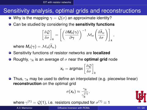
Sensitivity analysis, optimal grids and reconstructionsWhy is the mapping γ = Q(σ) an approximate identity?

Can be studied by considering the sensitivity functions[δQδσ

]k

=

[(∂Mn(γ)

∂γ

)−1

Mn

(δΛσδσ

)]k

,

where Mn(γ) =Mn(Λσ)

Sensitivity functions of resistor networks are localized

Roughly, γk is an average of σ near the optimal grid node

xk = argmax[δQδσ

]k

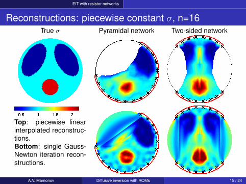
Thus, γk may be used to define an interpolated (e.g. piecewise linear)reconstruction on the optimal grid

σ(xk ) ≈ γk

γ(1)k

,

where γ(1) = Q(1), i.e. resistors computed for σ(1) ≡ 1A.V. Mamonov Diffusive inversion with ROMs 11 / 24


Sensitivity functions



Network topologies and optimal gridsPyramidal network Two-sided network

v1

v2

v3 v4

v5

v6

Circular planarnetworks do nothave to lookcircularOther topologiesare better suited forpartial dataproblemPyramidal: if BA issimply connectedTwo-sided: if BA isdoubly connectedBoth are well-connected andcriticalTop: networktopology; Bottom:optimal grid.



Reconstructions: smooth σ, n=16True σ Pyramidal network Two-sided network

Top: piecewise linearinterpolated reconstruc-tions.Bottom: single Gauss-Newton iteration recon-structions.



Reconstructions: piecewise constant σ, n=16True σ Pyramidal network Two-sided network

Top: piecewise linearinterpolated reconstruc-tions.Bottom: single Gauss-Newton iteration recon-structions.


CSEM with projection ROMs

Single measurement CSEM

Recall the CSEM equation

ut = ∇ · (σ∇u) = Aσu, in Ω, t > 0

with boundary conditions

u|BI = 0,∂u∂ν

∣∣∣∣BA

= 0

and an initial condition

u(x ,0) =

∫BA

φ(z)δ(x − z)dSz =

∫Ω

b(z)δ(x − z)dz, x ∈ Ω ∪ B,

with a transducer function b(z) satisfying supp b ⊆ BA

Let us consider a single measurement

yσ(t) =

∫Ω

b(z)u(z, t)dz



Projection-based model order reductionDefine the transfer function via Laplace transform

gσ(s) =

∫ +∞

0yσ(t)e−stdt = b∗(sI − Aσ)−1b, s > 0

Transfer function of a reduced model An ∈ Rn×n, bn ∈ Rn

gn(s) = b∗n(sIn − An)−1bn

Projection-based model reduction

An = V ∗AσV , bn = V ∗b, V ∗V = InThe n “columns” of V span the projection subspaceChoice of subspace is determined by matching conditions

[Mn(yσ)]k,j =∂k gσ∂sk

∣∣∣∣s=sj

=∂k gn

∂sk

∣∣∣∣s=sj

, j = 1, . . . ,m, k = 1, . . . ,2kj−1

at interpolation nodes sj ∈ [0,+∞) with

n =m∑

j=1

kj



Rational Krylov model order reductionPartial fraction expansion

gn(s) =n∑

j=1

cj

s + θj, cj > 0, θj > 0,

with negative poles −θj and positive residues cj

Rational gn, hence rational interpolation

Typical choices of projection subspaces in model reduction: rationalKrylov subspaces

Kn(s) = span

(sj I − Aσ)−k b | j = 1, . . . ,m; k = 1, . . . , kj

Popular special cases for forward modeling: moment matching

Kn(+∞) = span

b,Aσb, . . . ,An−1σ b

Kn(0) = span

A−1σ b,A−2

σ b, . . . ,A−nσ b

Kn(+∞) is bad for inversion



Connection to resistor networks: S-fraction formWrite the reduced model response as a Stieltjes continued fraction(S-fraction)

gn(s;γ) =1

γ−11 s +

1

γ−11 +

1. . . +

1γ−1

n s + γn

This is a boundary response w1(s) of a second-order finite differencescheme

γj (γj (wj+1 − wj )− γj−1(wj − wj−1))− swj = 0The coefficients γ = γj , γjn

j=1 are the analogue of the resistor networkcoefficientsThey are exactly the same for a rotationally symmetric circular networkOnce we have γ we can define

[Mn(γ)]k,j =∂k gn( · ;γ)

∂sk

∣∣∣∣s=sj



CSEM with multiple measurements: backscatteringTo deal with multiple measurements consider many transducerfunctions bα(z), α = 1, . . . ,p with disjoint supports supp bα ⊆ BA

For each α = 1, . . . ,p perform a rational interpolation

Mn(γα) =Mn(yασ )

and express the interpolant gαn (s;γα) as an S-fraction to obtain thecoefficients γα

Form a joint misfit functional out of all S-fraction coefficients

minimizeσ

p∑α=1

‖γα −Qα(σ)‖22 + µP(σ),

and solve with (a single step of) Gauss-Newton iteration

Reminder: the mapping Qα is defined as a chain

Qα : σ → yασ →Mn(yασ )→ Mn(γα)→ γα

Similarly to the resistor networks we can consider the sensitivityfunctions

[∂Qα

∂σ

]j , j = 1, . . . ,n



Sensitivity functionsSensitivity func-tions of γ−1

j (left)and γ−1

j (right) forj = 1, . . . , n (top tobottom), n = 5 fora single transducer(α = 4, yellow ) outof p = 8 (black ×).Simple Pade approx-imant at s = 60.Sensitivities resem-ble propagatingspherical waves.Higher s meanslower speed of prop-agation. Shouldavoid reflections fromboundaries.



Reconstructions: piecewise constant σTrue σ Reconstruction

Reconstuctions after a single Gauss-Newton iteration with a constant intialguess σ0 ≡ 1. Locations of p = 8 transducers are black ×.


Discussion

Conclusions and future workConclusions:

A framework of ROM-based inversion for diffusive problems is proposedIll-posed inverse problem is separated into two stages: ROMconstruction and reconstruction from ROM parametersThe instability is confined to ROM construction, it is controlled by ROMsizeThe reconstruction stage is formulated as a stable problem of minimizingthe ROM parameter misfitThe parameters are chosen so that they depend almost linearly on theunknown PDE coefficientThus the ROM parameter misfit minimization is close to quadratic andcan be solved with a single step of Gauss-Newton iteration

Future work:

EIT with resistor networks currently works in 2D or for limited subsets of3D data, a full 3D approach is yet to be developedROM-based CSEM inversion works in any dimension, but uses onlythe backscattering data


Discussion

References1 Electrical impedance tomography with resistor networks, L. Borcea, V.

Druskin and F. Guevara Vasquez. Inverse Problems 24(3):035013, 2008.2 Circular resistor networks for electrical impedance tomography with

partial boundary measurements, L. Borcea, V. Druskin andA.V. Mamonov, Inverse Problems 26(4):045010, 2010.

3 Pyramidal resistor networks for electrical impedance tomography withpartial boundary measurements. L. Borcea, V. Druskin, A.V. Mamonovand F. Guevara Vasquez, Inverse Problems 26(10):105009, 2010.

4 Study of noise effects in electrical impedance tomography with resistornetworks, L. Borcea, F. Guevara Vasquez and A.V. Mamonov,Inverse Problems and Imaging, 7(2):417-443, 2013.

5 Resistor network approaches to electrical impedance tomography,L. Borcea, V. Druskin, F. Guevara Vasquez and A.V. Mamonov,Inverse Problems and Applications: Inside Out II, Cambridge UniversityPress, 2012.

6 A model reduction approach to numerical inversion for a parabolicpartial differential equation, L. Borcea, V. Druskin, A.V. Mamonovand M. Zaslavsky, Inverse Problems 30(12):125011, 2014.


Date post:	08-Jun-2018
Category:	Documents
Upload:	dothuy
View:	215 times
Download:	0 times

Model order reduction for the numerical solution of ...mamonov/icerm2015talk.pdfModel order...

Documents