EUROMECH Colloquium 524 February 27 March 1, 2012 Multibody system modelling, control University of Twente and simulation for engineering design Enschede, Netherlands Model order reduction of non-linear flexible multibody models R.G.K.M. Aarts 1 * , D. ten Hoopen 1 , S.E. Boer 1 and W.B.J. Hakvoort 2 1 Faculty of Engineering Technology, University of Twente, Enschede, The Netherlands 2 Demcon Advanced Mechatronics, Oldenzaal, The Netherlands Keywords: Flexible multibody modelling, Reduced model order, Closed-loop simulations. In high precision equipment the use of compliant mechanisms is favourable as elastic joints offer the advantages of no friction and no backlash. For the conceptual design of such mechanisms there is no need for very detailed and complex models that are time-consuming to analyse. Nevertheless the models should capture the dominant system behaviour which must include relevant three-dimensional motion and geometric non-linearities, in particular when the system undergoes large deflections. In [1] we discuss a modelling approach for this purpose where an entire multibody system is mod- elled as the assembly of non-linear finite elements. The elements’ nodal coordinates and so-called defor- mation mode coordinates are expressed as functions of the independent (or generalised) coordinates q. With these expressions the system’s equations of motion are derived as a set of second order ordinary differential equations in terms of the kinematic degrees of freedom q, see e.g. [2] and the references therein: ¯ M (q)¨ q = D q F (x)T f - M D 2 q F (x) ˙ q ˙ q - D q F (e)T σ, (1) where ¯ M is the system mass matrix computed from the global mass matrix M . The notations D q F and D 2 q F denote so-called first and second order geometric transfer functions. The vector f are the nodal forces. Generalised stress resultants σ represent the loading state of each element. The sound inclusion of the non-linear effects at the element level appears to be very advantageous [2]. Only a rather small number of elastic beam elements is needed to model e.g. wire flexures and leaf springs accurately. Still it appeared that for a more complex compliant mechanism a rather large number of degrees of freedom is needed for an accurate model in the relevant frequency range [1]. Model order reduction techniques have been studied by several authors as these techniques offer a method to reduce the number of degrees of freedom while an accurate description of the dominant dynamic behaviour may be preserved. In the present paper we propose to describe the vibrational motion as a perturbation of a nominal rigid link motion. For order reduction a modal reduction technique is applied by expressing the perturbations of the degrees of freedom δq as δq = Vη, (2) where the elements of the vector η are the so-called principal coordinates and V is the modal matrix which is in general configuration dependent. Applying modal reduction the number of principal coor- dinates η is reduced representing only a rather small number of low frequency modes. Although the non-linear equations (1) still need to be integrated, we expect a gain in computational efficiency as large time steps can be applied in the absence of high frequent dynamic behaviour. Consider the two-link flexible manipulator shown in Figure 1. This manipulator has been introduced as a benchmark by Schiehlen and Leister [3] and has been quoted in several papers. Some properties are given in the table next to the figure. Joint angles φ 1 (t) and φ 2 (t) are prescribed with third order functions of time t moving from the initial to the final configuration in 0.5 s. Different from the original benchmark, we don’t include gravity in this paper. * Email: [email protected]1
Transcript
EUROMECH Colloquium 524 February 27 March 1, 2012Multibody system modelling, control University of Twenteand simulation for engineering design Enschede, Netherlands
Model order reduction of non-linear flexible multibody models
R.G.K.M. Aarts1∗, D. ten Hoopen1, S.E. Boer1 and W.B.J. Hakvoort21 Faculty of Engineering Technology, University of Twente, Enschede, The Netherlands
2 Demcon Advanced Mechatronics, Oldenzaal, The Netherlands
Keywords: Flexible multibody modelling, Reduced model order, Closed-loop simulations.
In high precision equipment the use of compliant mechanismsis favourable as elastic joints offer theadvantages of no friction and no backlash. For the conceptual design of such mechanisms there is noneed for very detailed and complex models that are time-consuming to analyse. Nevertheless the modelsshould capture the dominant system behaviour which must include relevant three-dimensional motionand geometric non-linearities, in particular when the system undergoes large deflections.
In [1] we discuss a modelling approach for this purpose wherean entire multibody system is mod-elled as the assembly of non-linear finite elements. The elements’ nodal coordinates and so-called defor-mation mode coordinates are expressed as functions of the independent (or generalised) coordinatesq.With these expressions the system’s equations of motion arederived as a set of second order ordinarydifferential equations in terms of the kinematic degrees offreedomq, see e.g. [2] and the referencestherein:
M(q)q = DqF(x)T
(
f −MD2qF
(x)qq)
−DqF(e)Tσ, (1)
whereM is the system mass matrix computed from the global mass matrix M . The notationsDqF andD
2qF denote so-called first and second order geometric transfer functions. The vectorf are the nodal
forces. Generalised stress resultantsσ represent the loading state of each element. The sound inclusionof the non-linear effects at the element level appears to be very advantageous [2]. Only a rather smallnumber of elastic beam elements is needed to model e.g. wire flexures and leaf springs accurately. Stillit appeared that for a more complex compliant mechanism a rather large number of degrees of freedomis needed for an accurate model in the relevant frequency range [1].
Model order reduction techniques have been studied by several authors as these techniques offera method to reduce the number of degrees of freedom while an accurate description of the dominantdynamic behaviour may be preserved. In the present paper we propose to describe the vibrational motionas a perturbation of a nominal rigid link motion. For order reduction a modal reduction technique isapplied by expressing the perturbations of the degrees of freedomδq as
δq = V η, (2)
where the elements of the vectorη are the so-called principal coordinates andV is the modal matrixwhich is in general configuration dependent. Applying modalreduction the number of principal coor-dinatesη is reduced representing only a rather small number of low frequency modes. Although thenon-linear equations (1) still need to be integrated, we expect a gain in computational efficiency as largetime steps can be applied in the absence of high frequent dynamic behaviour.
Consider the two-link flexible manipulator shown in Figure 1. This manipulator has been introducedas a benchmark by Schiehlen and Leister [3] and has been quoted in several papers. Some propertiesare given in the table next to the figure. Joint anglesφ1(t) andφ2(t) are prescribed with third orderfunctions of timet moving from the initial to the final configuration in0.5 s. Different from the originalbenchmark, we don’t include gravity in this paper.
Figure 1: Planar two-link manipulator: Initial configuration (1) and final configuration (2)with some of the parameters (adapted from [3]).
The motion of this manipulator has been computed with a non-linear model in which three flexiblebeam elements are used for each link. Each beam allows two bending modes yielding twelve dynamicdegrees of freedom in total. After the joint angles have reached their final values, a vibration of theelastic links is observed that is dominated by the lowest natural frequency of approximately3 Hz.
Next this simulation has been repeated with only a small number of time invariant modes that arecomputed with a modal analysis in the initial manipulator configuration. The results in Fig. 2(a) showthat with even only one mode the large scale motion at the tip is already described well. The detailedview near the upper extreme position reveals differences between the full order and reduced order sim-ulations. Including the time invariant second mode improves the accuracy and only a negligible errorremains. The computation time is reduced as no high frequency modes are present.
1 1.5 2
−0.4
−0.2
0
0.2
0.4
0.6
xtip
[t]
y tip [t
]
Non−linear2 modes1 mode
1 1.01 1.02
0.605
0.61
0.615
0.62
0.625
xtip
[t]
y tip [t
]
Non−linear2 modes1 mode
Figure 2: Motion of the manipulator tip during0.7 s: Full view (left) and detailed view (right)near the upper extreme position.
The example illustrates the possibilities offered by the proposed order reduction according to Eq. (2)combined with the solution of the non-linear equation of motion (1). It should be noted that in thisexample the mode shapes do not vary much along the prescribedtrajectory and the joint angles areprescribed. The application of the method to systems with controlled actuated joint angles and moresignificantly varying configurations is currently work in progress.
References[1] R.G.K.M. Aarts, J. van Dijk, D.M. Brouwer and J.B. Jonker, Application of flexible multibody modelling for
control synthesis in mechatronics, 10 pages in Multibody Dynamics 2011, ECCOMAS Thematic Conference,Ed. J.C. Samin, P. Fisette, Brussels, Belgium, July 4–7, 2011.
[2] J.B. Jonker, R.G.K.M. Aarts, and J. van Dijk,A linearized input-output representation of flexible multibodysystems for control synthesis, Multibody System Dynamics,21 (2) 99–122, 2009.
[3] W. Schiehlen and G. Leister,Benchmark-Beispiele des DFG-Schwerpunktprogrammes Dynamik vonMehrkorpersystemen, Universitat Stuttgart, Institut B fur Mechanik, Zwishenbericht ZB-64, 1991.
2
EUROMECH Colloquium 524 February 27 March 1, 2012Multibody system modelling, control University of Twenteand simulation for engineering design Enschede, Netherlands
(Re-)Starting a Generalized-α Solver for Constrained Systemswith Second Order Accuracy
Martin Arnold∗
Martin Luther University Halle-WittenbergNWF II – Institute of MathematicsD - 06099 Halle (Saale), Germany
Keywords: Efficient time integration, Generalized-α methods.
Abstract
Generalized-α time integration methods were originally designed for large scale problems in structuralmechanics [1] but may be used as well for constrained systems of moderate dimension that are typicalof multibody dynamics [2]. For constrained systems, the Newmark like update formula
qn+1 = qn + hvn + (0.5− β)h2an + βh2an+1 , (1a)
vn+1 = vn + (0.5− γ)han + γhan+1 (1b)
for position coordinates q and velocity coordinates v and the generalized-α update scheme
(1− αm)an+1 + αman = (1− αf )qn+1 + αf qn (1c)
for the auxiliary vectors an are coupled to equilibrium equations Mq = f −B>λ and constraintsΦ = 0 at t = tn+1:
In (1), the method parameters αf , αm, β, γ are chosen to satisfy the order condition γ = 12 + αf − αm,
see [1], and the time step size h is for the moment considered to be constant for all time steps tn → tn+1
:= tn + h.Following the principles of classical mechanics, the nΦ constraints (1e) are coupled to the dynamical
equations (1d) by constrained forces −B>(q)λ with B(q) := (∂Φ/∂q)(q) and Lagrange multipliersλ(t) ∈ RnΦ . All other forces and moments of the system are summarized in vector f = f(t,q,v). Themass matrix M(q) is assumed to be non-singular and symmetric, positive definite.
With an appropriate scaling of the corrector equations [3], the fixed step size implementation of (1)works well for reasonable time step sizes h > 0. The convergence analysis for h→ 0 proves stabilityand second order convergence if the stability conditions αm < αf < 1/2 and β > 1/4 + (αf − αm)/2are satisfied, see [4] and the extension to the generalized-α Lie group integrator of Bruls and Cardona[5] in [6]. Because of numerical damping, the generalized-α method (1) shows a favourable long-timebehaviour. But in a short transient phase, the method may suffer from large errors that are damped outrapidly, see Fig. 1.
In a recent joint work with O. Bruls (Liege) and A. Cardona (Santa Fe), this order reduction wasstudied in detail for a Lie group integrator [7]. The problem is fixed by perturbed initial values v0.
Figure 1: Spurious transient oscillations: Generalized-α method applied to benchmark Heavy top.
In the present paper, we study the extension of these results from the constrained case to (very) stiffunconstrained systems. Furthermore, the efficient (re-)initialization after discontinuities and a variablestep size algorithm with improved accuracy will be discussed.
References
[1] J. Chung and G. Hulbert. A time integration algorithm for structural dynamics with improvednumerical dissipation: The generalized-α method. ASME Journal of Applied Mechanics, 60:371–375, 1993.
[2] A. Cardona and M. Geradin. Time integration of the equations of motion in mechanism analysis.Computers and Structures, 33:801–820, 1989.
[3] C. Bottasso, O.A. Bauchau, and A. Cardona. Time-step-size-independent conditioning and sensitiv-ity to perturbations in the numerical solution of index three differential algebraic equations. SIAMJ. Sci. Comp., 29:397–414, 2007.
[4] M. Arnold and O. Bruls. Convergence of the generalized-α scheme for constrained mechanicalsystems. Multibody System Dynamics, 18:185–202, 2007.
[5] O. Bruls and A. Cardona. On the use of Lie group time integrators in multibody dynamics. J.Comput. Nonlinear Dynam., 5:031002, 2010.
[6] O. Bruls, A. Cardona, and M. Arnold. Lie group generalized-α time integra-tion of constrained flexible multibody systems. Mechanism and Machine Theory,doi:10.1016/j.mechmachtheory.2011.07.017, 2011.
[7] M. Arnold, O. Bruls, and A. Cardona. Improved stability and transient behaviour of generalized-αtime integrators for constrained flexible systems. Fifth International Conference on Advanced COm-putational Methods in ENgineering (ACOMEN 2011), Liege, Belgium, 14-17 November 2011,2011.
2
EUROMECH Colloquium 524 February 27 March 1, 2012
Multibody system modelling, control University of Twente
and simulation for engineering design Enschede, Netherlands
1
Modeling the Multibody Dynamics with the D&C System Simulator
Dmitry Balashov
* Oliver Lenord
Bosch Rexroth AG Bosch Rexroth AG
Rexrothstr. 3 Rexrothstr. 3
97816 Lohr am Main 97816 Lohr am Main
Germany Germany
Summary
The D&C System Simulator software is developed and deployed at the Bosch Rexroth AG to analyze
complex multi-domain engineering systems and to predict their hydraulic, electric or mechanical
behavior. The underlying numerical model and key features of the multi body dynamics module that
is a part of the entire software package are outlined in this paper. The multi body 3D model is
assumed as an arbitrary system of rigid bodies connected by mechanical joints and subjected to
mechanical loads. Kinematic chains, over-constrained systems and models with active control units
are featured by this simulation tool. The minimum dimension order-N algorithm [1] is used to
calculate the multi body dynamic response. A simulation example is presented.
What is the D&C System Simulator?
Development of the dynamic simulation software is motivated by the need of accurately modelling a
variety of industrial products and prototypes at the Bosch Rexroth AG such as hydraulic and
pneumatic actuators, chain conveyors, rail transportation and linear motion systems, production
platforms, wind turbines, solar plants and industrial robots. Typical problems related to the
performance and functionality verification; tuning and evaluation of the optimum design parameters;
noise, vibration and harshness issues; technical deficiencies can be analyzed and resolved using the
sophisticated software tool. This reflects a main challenge to develop the dynamic simulation software
D&C System Simulator which is suitable for the multi disciplinary models incorporating standard
hydraulic components such as pumps or valves and multi body mechanical systems with arbitrary
geometry and topological configuration.
The simulator core accounts a set of libraries with standard components matching different physical
domains: hydraulic, electric, 1D mechanic, analog, logic, digital and 3D multi body. An interactive
model set up is split into two separate steps: drawing the 1D diagram with e.g. hydraulic pipelines and
a control circuit and creation of the 3D multi body subsystem. The both models are coupled via the
input/output ports implementing an interface between the mechanical state variables and the actuating
forces. Graphical set up of the 1D diagram is provided by positioning icons associated with the model
components and drawing the connectors between them in a manner that is very similar to the
Matlab/Simulink software. A 3D multi body model can be generated using a graphical user interface
with space representation of the mechanical parts connected by joints and optionally applied motion
generators. The items causing forces or torques can be attached to the selected points on the bodies.
From a mathematical point of view, dynamics of the entire multi domain model is governed by the
common system of differential algebraic equations (DAE) while a time integration of this DAE
system is performed by the solver object. The runtime simulation core (the model libraries, the solver
and their interfaces) is implemented in native C++ using an object oriented approach while the dialogs
and graphical user interface controls are implemented in C#. A sophisticated 3D graphics modeling
and animation facility is developed using the Open GL graphics library.
EUROMECH Colloquium 524 February 27 March 1, 2012Multibody system modelling, control University of Twenteand simulation for engineering design Enschede, Netherlands
Sensitivity analysis for flexible multibody systemsformulated on a Lie group
Olivier Bruls∗ and Valentin Sonneville†
University of LiegeDepartment of Aerospace and Mechanical Engineering
Chemin des Chevreuils 1, Building B52,4000 Liege, Belgium
Keywords: Lie group formalism, sensitivity analysis, direct differentiation method, adjoint variablemethod, optimization.
The sensitivity of the dynamic response of a multibody system is a key information in gradient-baseddesign optimization and optimal control problems. The present contribution addresses the computationof the sensitivities for systems which naturally evolve on a Lie group and not on a linear space.
The Lie group framework offers a number of advantages for the analysis of systems with large rota-tions variables [4, 5], e.g. for finite element models of systems with rigid bodies, kinematic joints, beamsand shells. Firstly, the equations of motion are derived and solved directly on the nonlinear manifold,without an explicit parameterization of the rotation variables, which leads to important simplificationsin the formulations and algorithms. Secondly, displacements and rotations are represented as incre-ments with respect to the previous configuration, and those increments can be expressed in the material(body-attached) frame. Therefore, geometric nonlinearities are automatically filtered from the relation-ship between incremental displacements and elastic forces, which strongly reduces the fluctuations ofthe iteration matrix during the simulation [3].
Classical sensitivity analysis methods include finite difference methods, semi-analytical approachesor automatic differentiation. Semi-analytical approaches have interesting properties in terms of accuracy,robustness and computational cost. They have been successfully exploited for dynamic systems evolvingon a linear parameter space, for which classical ODE or DAE solvers are available [1, 2]. However, tothe best of our knowledge, the sensitivity analysis of dynamic systems on a Lie group has not beenaddressed in literature and deserves some particular investigations.
In a previous work [6], a direct differentiation method was proposed for systems evolving on SO(3),the group of finite rotations. Here, the study is extended to a more general class of dynamic systems withkinematic joints, whose equations of motion have the structure of a DAE on a Lie group. It is shownthat the nonlinearity of the Lie group and of the time integration formulae need to be carefully treatedfor the development of accurate sensitivity analysis algorithms.
A broad class of semi-analytical methods, including the direct differentiation method and the adjointvariable method, is discussed in the presentation. The main properties of those methods, which arewell-known for problems on a linear space, are also observed for problems on a Lie group. Accuratesensitivity analysis algorithms are established and implemented in a simple way, exploiting the compactand elegant Lie group formalism. Their performance is studied for academic examples as well as for theoptimization of structural components using topology and/or shape optimization techniques.∗Email: [email protected]†Email: [email protected]
1
References
[1] D. Bestle and P. Eberhard. Analyzing and optimizing multibody systems. Mechanics of Structuresand Machines, 20:67–92, 1992.
[2] D. Bestle and J. Seybold. Sensitivity analysis of constrained multibody systems. Archive of AppliedMechanics, 62:181–190, 1992.
[3] O. Bruls, M. Arnold, and A. Cardona. Two lie group formulations for dynamic multibody systemswith large rotations. In Proceedings of the IDETC/MSNDC Conference, Washington D.C., U.S.,August 2011.
[4] O. Bruls and A. Cardona. On the use of Lie group time integrators in multibody dynamics. ASMEJournal of Computational and Nonlinear Dynamics, 5(3):031002, 2010.
[5] O. Bruls, A. Cardona, and M. Arnold. Lie group generalized-α time integration of constrainedflexible multibody systems. Mechanism and Machine Theory, in press.
[6] O. Bruls and P. Eberhard. Sensitivity analysis for dynamic mechanical systems with finite rotations.International Journal for Numerical Methods in Engineering, 74(13):1897–1927, 2008.
2
EUROMECH Colloquium 524 February 27 March 1, 2012Multibody system modelling, control University of Twenteand simulation for engineering design Enschede, Netherlands
Calculating Input Data for Multibody System Simulation by Solving anInverse Control Problem
Michael Burger∗
Fraunhofer Institute for Industrial and Financial Mathematics (ITWM)Fraunhofer Platz 1, 67663 Kaiserslautern, Germany
In order to simulate a multibody system (MBS) model of a real mechanical system, input data (or drive-signals) is needed to excite the numerical model in such a way that the simulated loads are as closeas possible to the loads that act on the real system under operational conditions. If such input data isavailable, numerical system simulation of MBS models can be used very efficiently in many applicationareas. For instance, in vehicle engineering, during the development process of a full vehicle or specificcomponents, different designs and constructions can be analyzed and optimized by numerical simulationof a computer (MBS) model, see [3].
However, such input data with suitable properties is often not available. In case of vehicle engineer-ing, a convenient example for input data is a digital road profile, which has an additional very desirableproperty: it is invariant w.r.t. the vehicle model. That is, a digital road profile can be used to excitedifferent vehicles, it does not depend on a specific variant. Unfortunately, as indicated, digital roadprofiles are hard to obtain; of course, a real road can be measured and digitalized, but this is costly,time-consuming and requires complex sensor techniques.
In contrast to this, during a typical test-track drive of a prototype vehicle, a lot of quantities withinthe vehicle are measured and stored comparably easy and by default without additional effort. Whence,the obvious task arise to derive input data with suitable properties, e.g., a road profile, on the basis oftypically measured inner vehicle quantities, such as accelerations of specific components or the forcesand torques that act on the vehicle’s spindles.
This task leads to the following mathematical problem formulation, cf. [1]. Assume that there is areal mechanical system, e.g., a full vehicle, and a mathematical description as MBS model, i.e., thecorresponding equations of motion, e.g., in the following well-known form:
M(q)q = f(t, q, q, u)−GT (q)λ
0 = g(q),(1)
with generalized coordinates q ∈ Rnq , Lagrange multipliers λ, a positive definite mass matrix M(q)and G(q) := ∂g/∂q being of full row rank. The vector f subsumes all acting forces and torques and, inaddition to that, it includes the dependence on the desired, but unknown, input quantity u ∈ Rnu . Last,not least, suppose that the measured quantities, denoted by zREF : [0;T ] → Rnz as functions of time,correspond to system outputs zout, defined by
where h is a smooth vector function. With these notions, we are faced with the following inverse controlproblem, fig. 1:
Find u ∈ D such that ‖zout − zREF ‖ = ‖h(t, q, q, u)− zREF ‖ → min, (3)
where (q, q) is the solution of eq. (1) with the input u and D is a suitable domain for input functions.
In this contribution, we will present an operator-theoretic framework to precisely formulate the aboveinverse control problem. We introduce an input-output-operator Ph that maps each input u to the corre-sponding output,
Ph(u) = zout. (4)
We discuss some properties of this operator like continuity and differentiability and interpret these no-tions in the context of perturbations. These results are derived and proven in [1]. The inverse controlproblem from above leads to the question wether or not the input-output-operator is invertible at zREF .We summarize several approaches to (computationally) solve the inverse control problem - for a detaileddiscussion, we refer to [1].
We end with a numerical case study, in which the operator-theoretic framework as well as some ofthe computational solution methods is applied to compute a virtual road profile for full-vehicle simu-lation, see also [1, 2]. In this case study, a specific subsystem technique is introduced that allows toreduce the inverse-control problem to a subsystem of moderate complexity when compared to the fullvehicle MBS model, which is built up in a commercial software tool. This subsystem approach is brieflysketched, a detailed description, discussion and proofs can be found in [1].
Figure 1: Input-Output Configuration
References
[1] M. Burger. Optimal Control of Dynamical Systems: Calculating Input Data for Multibody SystemSimulation. Dissertation. TU Kaiserslautern. 2011. To appear.
[2] M. Burger, K. Dressler, and M. Speckert. Invariant Input Loads for Full Vehicle Multibody SystemSimulation. In Multiobody Dynamics 2011 ECCOMAS Thematic Conference, Brussels, 2011.
[3] K. Dressler, M. Speckert, and G. Bitsch. Virtual test rigs. In C. Bottasso, P. Masarati, and Trainelli,editors, Multibody dynamics 2007, Eccomas Thematic Conference, Milano, Italy, 25-28 June.
2
EUROMECH Colloquium 524 February 27 March 1, 2012
Multibody system modelling, control University of Twente
and simulation for engineering design Enschede, Netherlands
1
Complete dynamic balancing of a 3-DOF spatial parallel mechanisms by
Figure 1: Illustrative designs of CaPaMan 2bis: a) original design; b) proposed balanced design
Dynamic balancing has been accomplished by imposing the usual shaking force balance condition,
indicating that the general centre of mass of the systems remains static, and the shaking moment
balance condition as a constant global angular momentum during motion.
Simulation results
By the application of the previous described technique a new design has been obtained and is
presented as an ADAMS model in Fig. 1b (crown wheels of the gear systems have been omitted).
This model has been tested by applying a very simple torque law to actuators to move the mobile
platform in straight line up and down in 2 seconds with cranks from -35° to 35° and back. Fig. 2a
shows the resulting shaking force with its components, and Fig. 2b shows shaking moment
components.
a) b)
Figure 2: Numerical results of balancing CaPaMan 2bis: a) shaking force components; b) shaking
moment components
References [1] G. G. Lowen, F. R. Tepper and R. S. Berkof, Balancing of Linkages - An Update, Mechanism
and Machine Theory, 18(3), pp. 213–220, 1983.
[2] V. Arakelian, M. Dahan and M. R. Smith, A Historical Review of the Evolution of the Theory of
the Balancing of Machines, pp. 291–300 in Proceedings of the International Symposium on
History of Machines and Mechanisms - HMM2000, Ed. Ceccarelli, M., Italy, 2000.
[3] C. Gosselin, Static Balancing and Dynamic Balancing of Parallel Mechanisms, pp. 291–300 in
Smart Devices and Machines for Advanced Manufacturing, Ed. , Wang, L. and Xi, J., London,
2008.
[4] V. van der Wijk and J. Herder, Synthesis of Dynamically Balanced Mechanisms by Using
Counter-Rotary Countermass Balanced Double Pendula, ASME Journal of Mechanical Design,
131(11), 2009.
EUROMECH Colloquium 524 February 27 March 1, 2012Multibody system modelling, control University of Twenteand simulation for engineering design Enschede, Netherlands
State Estimation Using Multibody Models and Unscented Kalman Filters
Roland Pastorino∗
Javier CuadradoUniversity of La Coruna
Mendizabal, s/n 15403 Ferrol, Spain
Dario Richiedei†
Alberto TrevisaniDTG, Universita degli Studi di Padova
Stradella S. Nicola 3 - 36100 Vicenza, Italy
Keywords: nonlinear state observers, multibody models, unscented Kalman filters.
1 Introduction
Over the last years, state estimation in mechanical systems has gained interest with the recent devel-opment of real-time state estimation using MBSs (Multibody Systems). In practice, the knowledge ofthe system’s states allows to improve the closed-loop performances of it, reducing the use of expensivesensors by replacing them with virtual sensors, and finally improving reliability by making the systemfault tolerant.
On the one hand, numerous works address the synthesis of optimal observers for linear mechanicalsystems through the KF (linear Kalman Filter). On the other hand, when nonlinear mechanical systemsare considered, such as MBSs, only sub-optimal approaches based on the LKF (Linearized KF) haveusually been adopted to ensure high-frequency and hard real-time estimation. Indeed, up to now, the useof other types of nonlinear observers using MBSs has only been investigated marginally. The lack ofsuch observers in this field of engineering is mainly due to the difficulty in performing fast integration ofthe nonlinear equations of motion for MBSs, which usually involve high frequency dynamics and severenonlinearities. In [1], it is shown how the improvements in multibody dynamics raise the possibilityto employ complex models in real-time state observers. The estimation was performed through theEKF (Extended KF) in its continuous form (also known as EKBF (Extended Kalman-Bucy Filter)).Generally speaking, the EKF is the most widely used algorithm for nonlinear estimation. It makes useof the nonlinear system model to perform the time update, but propagates the mean and covarianceof the states through the linearized model. As long as the system remains linear on the timescale ofthe updates, the linearization error and consequently the estimation error stay small and accuracy isguaranteed. However, when nonlinearities are severe, EKF often gives unreliable or divergent estimates.On top of that, the linearization requires a Jacobian matrix which could either be difficult to calculate ornot exist. Implementation difficulties are particularly relevant if the system model is modeled by DAE(Differential Algebraic Equations) as it is common in MBSs.
Recent developments in Kalman filtering algorithms make possible to overcome part of the EKFshortcomings. The SPKFs (Sigma-Point Kalman Filters), also called LRKFs (Linear Regression KalmanFilters), use a set of deterministically calculated weighted samples, also named sigma-points or even re-gression points [2]. This set has to capture at least the first and second order moments of the actual stateprobability distribution. Each sigma-point is then individually propagated through the nonlinear systemequations. The posterior statistics are approximated using simple functions involving the transformedsigma-points. Thereby, this approximation, that does not require the calculation of a Jacobian matrix,is more accurate than the EKF linearization. Different sigma-point set definitions lead to different fil-ter characteristics that allow to give priority to estimation accuracy or to computational efficiency. The∗Email: [email protected]†Email: [email protected]
1
most famous variants are the UKF (Unscented KF), the CDKF (Central Difference KF) [2], the SSUKF(Spherical Simplex UKF) [3] and their respective square-root forms which allow to improve the numer-ical stability. Therefore, a natural approach to overcome the EKF problems when employing multibodymodels would be to use SPKFs. To the best of the authors’ knowledge, UKFs have never been appliedto the estimation of multibody models.
2 Using multibody models in Unscented Kalman filters
The aim of this work is to present the first implementation of UKFs using multibody models and todiscuss their performances. The objective is not to define all the possible ways of using multibodymodels in UKFs but to present the most relevant. As the multibody formulation is involved, the state-space reduction method known as matrix-R method is employed to convert the DAE of the multibodymodel into an ODE with a dimension equal to the number of degrees of freedom of the system, as in [1].Both implicit and explicit integration schemes have been used. The filters’ state vector has been chosenequal to the vector of independent coordinates in order to minimize the number of sigma-points. For thesake of simplicity, additive white Gaussian noise has been considered. The selection of such a multibodyformulation and such a state vector leads to a straight-forward implementation of the observer with adirect physical significance that is valid for all the SPKFs. Performance comparisons between UKFs,SSUKFs, their square-root forms and EKBFs have been carried out in simulation on a 5-bar linkage.The mechanism’s parameters have been obtained from an experimental 5-bar linkage and the sensor’scharacteristics from off-the-shelf sensors to reproduce a realistic simulation.
3 Conclusion
This work presents the development of nonlinear state observers based on the UKF family, that usemultibody models. Although these filters largely outperform the accuracy of the EKBF by using betterapproximations of system nonlinearities, the computational cost related to the sigma-points is high. As aconsequence, the choice of the most suitable filter depends on the application requirements and is a tradeoff between estimation accuracy and computational efficiency. Future works will be devoted to deeperinvestigations on a wider class of multibody formulations and filters, and to the experimental validationof the proposed observers.
Acknowledgements
The authors would like to thank the Spanish Ministry of Science and Innovation and ERDF funds throughthe grant TRA2009-09314 for its support in this research.
References
[1] J. Cuadrado, D. Dopico, A. Barreiro, E. Delgado, Real-time state observers based on multibodymodels and the extended Kalman filter, Journal of Mechanical Science and Technology, 23(4), pp.894–900, 2009.
[2] Julier, S.J., Uhlmann, J.K., Unscented filtering and nonlinear estimation, in Proceedings of theIEEE, 92(3), pp. 401–422, 2004.
[3] Julier, S.J., The spherical simplex unscented transformation, in Proceedings of the American ControlConference, (3), pp. 2430–2434, 2003.
2
EUROMECH Colloquium 524 February 27 March 1, 2012Multibody system modelling, control University of Twenteand simulation for engineering design Enschede, Netherlands
Model Reduction of Large Scaled Industrial Modelsin Elastic Multibody Systems
Peter Eberhard∗
Institute of Engineeringand Computational Mechanics
University of Stuttgart
Michael FischerInstitute of Engineering
and Computational MechanicsUniversity of Stuttgart
Keywords: model order reduction, elastic multibody systems, LU-decomposition, high performancecomputing, out-of-core solution.
Introduction
The description of the dynamical behavior of mechanical systems is of great interest in the developmentprocess of technical products. If rigid body movements and additional elastic deformations have tobe concerned, the method of elastic multibody systems (EMBS) is used. With the floating frame ofreference formulation, the movement of an elastic body is separated into a huge nonlinear motion of thereference frame and a small elastic deformation with respect to this reference frame.
The discretization of the elastic body with finite elements provides a linear time-invariant secondorder multi input multi output (MIMO) system
M e · q(t) +De · q(t) +Ke · q(t) = Be · u(t),y(t) = Ce · q(t)
(1)
with the symmetrical sparse mass matrix M e, damping matrix De, stiffness matrix Ke, inputs u(t),outputs y(t) and states q(t).
In industrial applications large finite element models with millions degrees of freedom are generatedto describe the elastic behavior. To enable the simulation of EMBS with large models, the degreesof freedom of the elastic body have to be reduced by approximating the nodal displacements with thehelp of ansatz functions. Modern reduction methods, like Krylov-subspace based moment matching orGramian matrix based reduction, as described in [1], are used to find the optimal ansatz functions.
Main Calculation Step in Model Reduction
The main calculation step in modern reduction techniques is the solution of large sparse symmetric linearsystems
A ·X = B (2)
with the large sparse matrix A ∈ CN×N , the right hand side B ∈ CN×r and the solution X ∈ CN×r.There are two possibilities to solve sparse linear systems, either to use a direct or an iterative solver.
The iterative solver needs multiple steps to solve the system. This allows to store only one column of Xand B in the solving process. In contrast, the direct method solves Equation (2) by a decomposition ofA, like LU-factorization, and a following forward elimination and backward substitution. For large righthand sides, which is common in using Krylov-subspace based model reduction, the LU-decomposition,
in contrast to the iterative method, is calculated only once. However, the LU-decomposition requires tostore the lower triangular matrix L ∈ CN×N and upper triangular matrix U ∈ CN×N . Because of thefill-ins these matrices have more nonzero entries than the corresponding part of A. The large memoryconsumption of the LU-decomposition is the biggest numerical challenge in reducing large models.
Solving Process
At the Institute of Engineering and Computational Mechanics the software package Morembs [2] isdeveloped to reduce the elastic degrees of freedom. This software is implemented in Matlab and C++.In the C++ Version different numerical libraries for solving large linear sparse systems are tested in thiscontribution. The different direct solvers are compared in [3]. In Morembs, freely available librariesare preferred. Therefore, well tested numerical libraries for the LU-decomposition, like Umfpack [4] orMumps [5], are used.
Although using the most efficient direct solvers, the memory hardware limits the size of modelswhich can be reduced in Morembs. One possibility to solve large systems with Morembs is using super-computers. Therefore, a NEC SX-9 supercomputer at the High Performance Computing Center Stuttgartis used. The computation cluster allows a memory allocation of 512 GB. Morembs is a sequential pro-gram which runs slow on the vector supercomputer. On the newly installed faster supercomputer CrayXE6 Morembs runs faster but needs more time than the program needs on a serial standard computer(Intel-Xeon Quadcore, 2.4 GHz, 6 GB RAM). Furthermore, the usage of supercomputers is expensiveand not all users have access to such supercomputers.
Some numerical direct solver packages, like Mumps, feature an Out-of-Core capability. This allowsthe solution of very large sparse linear systems with a standard computer by storing most parts of thelower and upper triangular matrices on the hard drive. With a solid-state-drive the reduction with theOut-of-Core solver Mumps is slower than the time reducing the model in-core but it is nearly four timesfaster than the serial reduction on the supercomputer. This allows the model reduction of large scaledindustrial models with millions degrees of freedom on standard computers in a reasonable time.
References
[1] Lehner, M.: Modellreduktion in elastischen Mehrkorpersystemen (in German). Dissertation,Schriften aus dem Institut fur Technische und Numerische Mechanik der Universitat Stuttgart,Band 10. Aachen: Shaker Verlag, 2007.
[2] Fehr, J.; Eberhard, P.: Simulation Process of Flexible Multibody Systems with Non-modal ModelOrder Reduction Techniques. Multibody System Dynamics, Vol. 25, No. 3, pp. 313–334, 2011.
[3] Gould, N.I.M.; Scott, J.A.; Hu, Y.: A numerical evaluation of sparse direct solvers for the solutionof large sparse symmetric linear systems of equations. ACM Transactions on MathematicalSoftware, Vol. 33, No. 2, p. 10, 2007.
[4] Davis, T.A.: Algorithm 832: UMFPACK, an unsymmetric-pattern multifrontal method. ACMTransactions on Mathematical Software, Vol. 30, No. 2, pp. 196–199, 2004.
[5] Amestoy, P.; Duff, I.; Robert, Y.; Rouet, F.; Ucar, B.: On computing inverse entries of asparse matrix in an out-of-core environment. Technical report rt-apo-10-06, Institut nationalde recherche en informatique et en auotmatique, 2010.
2
EUROMECH Colloquium 524 February 27 March 1, 2012
Multibody system modelling, control University of Twente
and simulation for engineering design Enschede, Netherlands
1
A Planar Multibody Lumbar Spine Model for Dynamic Analysis
Sara Tribuzi Morais
*, Paulo Flores
†, J.C. Pimenta Claro
‡
CT2M / Departamento de Engenharia Mecânica, Universidade do Minho
Campus de Azurém, 4800-058 Guimarães, Portugal
Keywords: Biomechanics, spine, low back pain, multibody lumbar model.
Extended Abstract
The human vertebral column is a complex system, which main functions are: (i) transferring
weight and the resultant bending moments of the head, trunk, and any weights being lifted to the
pelvis; (ii) allowing physiologic relative motions between the aforementioned anatomical elements;
(iii) protecting the spinal cord from damaging actions produced by physiologic movements and/or
trauma; and (iv) providing the attachment points for muscles and the ribcage [1]. Thus, the spine has
been identified as one of the most susceptible human body parts to suffer traumatic and degenerative
pathologies. The World Health Organization and the Portuguese Ministry of Health report chronic
rheumatic diseases as the most frequent group of illnesses in developed countries, and low back pain
(LBP) as the most common spinal disorder in this group. Lumbar disc degeneration (LDD) was
identified as one of the main causes of LBP [2]. A frequently applied solution for LDD is
intervertebral fusion, in which two vertebrae are fused together. However, this medical procedure has
a consequence of limiting the spinal range of motion due to the elimination of the intervertebral disc
(IVD) function.
The spine is composed by 33 vertebrae (24 articulating and 9 fused) and can be divided in five
regions: cervical, thoracic, lumbar, sacral and coccygeal. However this study will be focus on the
lumbar spine region, where the structure is subjected, and have to support, the highest network loads.
The main objective is to build up a general two-dimensional multibody methodology able to model,
analyze and simulate the dynamic behavior of the human lumbar spine system – in terms of vertebras,
ligaments and the IVD itself – as a basis for future applications in the study of pathological and non-
pathological situations , as well as in the evaluation of load and displacement performance under work
of the IVD, suitable for the analysis and design of substitution implants.
contact
Sacrum
(a) (b)
L1
L2
L3
L4
L5
process
Facet joint
Spinous
Lu
mb
ar ve
rte
bra
e
x
y
(i)
(j)
hi
xi
hj
xj
IVD
Oj
Oi
SSL
LF
ISL PLL ALL Potential
element Bushing
Figure 1: (a) Schematic representation of the lumbosacral spine; (b) Multibody model of the consecutive vertebrae with their
fundamental elements (bodies, ligaments, bushing elements, potential contact areas).
The multibody spine model considered in the present work includes six rigid bodies, representing
the sacral structure and five lumbar vertebrae, as it is illustrated in Figure 1(a). The fundamental
geometric data used to build this multibody model is based on the material available in the literature,
namely, in the works by Panjabi [3] and Monteiro [4]. For the definition of the vertebra it is important
to define a body-local coordinate system of each element that is located at the body center of mass, as
Figure 1(b) shows. The bodies of the system are considered to be rigid and kinematically constrained
by an ideal revolute joint located the facet joints, as it is represented in Figure 1(b). This restriction
allows the relative flexion-extension motion and some compression-tension in the IVDs. Bushing
elements of linear and rotational types are used to model the IVDs, which act as a spring-damper
components. For this purpose, translational and rotational stiffness and damping properties are
included in a penalty approach to model the bushing elements [4]. In turn, the ligaments are modeled
as simple nonlinear spring, which work in two different regimens according to the ligament strain
during relative motion. The main ligaments considered in the spine model are shown in Figure 1(b).
Furthermore, possible contact events can take place between adjacent spinous processes. This
contact scenario is modeled as a contact between a spherical surface and a planar surface, as it is
illustrated the Figure 1(b). The contact-impact forces are computed by employing a continuous
contact force model, based on the elastic Hertz theory, together with a dissipative term associated with
the internal damping [5]. The selection of an appropriate contact force model is of paramount
importance in the measure that the contacting bodies are characterized by high damping properties.
The formulation of multibody system dynamics adopted in this work uses the generalized
Cartesian coordinates and the Newton-Euler approach to derive the equations of motion. This
formulation results in the establishment of a mixed set of partial differential and algebraic equations,
which are solved in order to predict the dynamic behavior of multibody systems. The Newton-Euler
approach is very straightforward in terms of assembling the equations of motion and providing all
joint reaction forces. Additionally, the equations of motion are solved by using the Baumgarte
stabilization technique with the intent of keeping the constraint violations under control [6].
The forces developed at the potential contact areas located at the spinous processes, the restive
force and moments associated with the bushing elements and the force produced in the ligaments are
introduced into the system’s equations of motion as external generalized forces. Finally, results in
terms of the dynamic simulations of the multibody spine model described above are used to
demonstrate the accuracy and efficiency of the presented approach and to discuss the main
assumptions and procedures adopted.
Acknowledgement
This work is part of the ‘NP Mimetic - Biomimetic nano-fiber-based nucleus pulposus
regeneration for the treatment of degenerative disc disease’ research project, funded by the European
Commission under the Seventh Framework Programme (FP7).
References
[1] A.A. White, M.M. Panjabi, Clinical biomechanics of the spine, Lippincott, Philadelphia,
1990.
[2] K. Luoma, H. Riihimäki, R. Luukkonen, R. Raininko, E. Viikari-Juntura, A. Lamminen, Low
Back Pain in Relation to Lumbar Disc Degeneration, Spine, 25(4), pp. 487-492, 2000.
[3] M.M. Panjabi, V. Goel, T. Oxland, K. Takata, J. Duranceau, M. Krag, M. Price, Human
lumbar vertebrae. Quantitative three-dimensional anatomy, Spine, 17(3), pp. 299-306, 1992.
[4] N. Monteiro, Analysis of the Intervertebral Discs Adjacent to Interbody Fusion using a
Multibody and Finite Element Co-Simulation, MSc Thesis, Mechanical Engineering
Department, Technical University of Lisbon, 2009.
[5] P. Flores, M. Machado, M.T. Silva, J.M. Martins, On the continuous contact force models for
soft materials in multibody dynamics, Multibody System Dynamics, 25, 357-375, 2011.
[6] P.E. Nikravesh, Computer-aided analysis of mechanical systems, Prentice-Hall, 1988.
EUROMECH Colloquium 524 February 27 March 1, 2012Multibody system modelling, control University of Twenteand simulation for engineering design Enschede, Netherlands
Trajectory Planning Optimization of Mechanisms with RedundantKinematics for Manufacturing Processes with Constant Tool Speed
Andreas Scholz∗ Francisco Geu Flores† Andres Kecskemethy‡
Chair of Mechanics and Robotics, University of Duisburg-Essen,Lotharstr. 1, 47057 Duisburg, Germany
Optimal path planning techniques for kinematically redundant mechanisms havebeen throughly studiedin the past ([1]). A common practice to find possible solutions with commercial software is to formulatethe problem as a nonlinear optimization problem ([2]) and solve it using standard SQP-methods. Amajor task is hereby to formulate the optimization problem such that convergence is guaranteed.
The present paper describes a three-step optimization method to compute the optimal controlanddesign of mechanisms with redundant kinematics for tasks requiring constant tool velocities along givenspatial trajectories defined with respect to one of the moving links. The solution approach consists indescribing the kinematics of the system as a one-parametric function of the motion of the tool alongthe workpiece and parametrizing the motion of the redundant joints as a spline function of this oneparameter. The optimal control problem is therefore transformed into a nonlinear optimization problemwith the spline coefficients as optimization parameters, which can be solved by SQP routines.
Three-stage optimization method
The method is presented by means of an application example (see figure below), comprising a planarserial robot with three degrees of freedomθ ∈ IR3, as well as an auxiliary mechanism with one rotationaldegree of freedomϕ around an axis normal to the robot working plane. The robot carries thetool atits end effector whilst the auxiliary mechanism carries the workpiece. The goal is to find the optimalcontrolsθ(t) andϕ(t) of the robot and the auxiliary mechanism, respectively, as well as the optimalrelative pose of the mechanism with respect to the robot inertial coordinatesystemK0, which allowfor a maximal constant tool speeds along a given pathS on the workpiece, subject to the maximallyallowed joint angular displacements, velocities, and accelerations.
The kinematics of both mechanisms is described as a one-parametric function of the path parameters, by (1) interpolating the relative motion of the tool with respect to the given trajectory S using aDARBOUX-frame parametrization scheme, and (2) by parametrizing the motion of the redundant degreeof freedomϕ as a spline functionϕ(s) of third order. To this end, the problem is formulated as anonlinear optimization problem with the relative pose of the auxiliary mechanism with respect to therobot, the constant speeds of the tool along the given trajectory, and the spline coefficients ofϕ(s)as optimization parameters. The optimal parameters are sought by means of a three-stage optimizationmethod. Each stage uses the optimal solution of the previous stage as an initial guess.
Figure 1: Optimal motion of the robot and the auxiliary mechanism
The first stage consists in searching for a feasible initial guess by minimizing the standard deviationof the joint angles during the motion. In this stage, a low constant speeds along the path as well as alow number of spline segments ofϕ(s) are prescribed, and the velocity and acceleration constraints atthe robot joints are ignored. In the second stage, the number of spline segments is refined (in our case to150 segments) and the sum of squared values of the angular velocities andaccelerations is minimized.Furtheremore, the maximally allowed angular displacements, velocities and accelerations at the robotactuators, as well as the determinant of the transmission JACOBIAN are regarded as constraints. The thirdstage consists of a sequence of optimization runs with the same cost and constraint functions of stagetwo, but with increasing tool speeds at each new step. Hereby, the tool speed is increased manuallyin small increments such that the optimizer can correct the respective constraint violations and the toolspeeds approaches asymptotically its maximal value.
The figure shows the optimal solution for the presented example. The blue dashed curved representsthe prescribed pathS on the workpiece, whereas the red curve depicts the motion of the end effectorwith respect toK0. It can be seen directly that bothθ3 andϕ reach their limits during the trajectory,hence the mechanism cannot be driven with a higher tool speeds. The auxiliary mechanism supportsthe robot such that the motion takes place widely inside the robot working space, allowing for a higherconstant tool speeds along the given trajectory.
Conclusions
This paper addresses the optimal control of mechanisms with redundant kinematics for tasks requiringconstant tool velocities along given spatial trajectories. A three-stage optimization method has beenpresented by means of an application example. The paper shows that the method yields good conver-gence properties, allowing for the determination of the minimal process cycle time. For future researchit is planned to automize stage 3 of the procedure and to compare the currentapproach with collocationmethods such as [2].
References
[1] D. P. Martin, J. Baillieul, and J. M. Hollerbach. Resolution of Kinematic Redundancy Using Op-timization Techniques. InIEEE Transactions on Robotics and Automation, volume 5, no. 4, pages529–533, August 1989.
[2] Oskar von Stryk. Numerical Solution of Optimal Control Problems by Direct Collocation. InOptimal Control, (International Series in Numerical Mathematics 111, pages 129–143, 1993.
2
EUROMECH Colloquium 524 February 27 March 1, 2012Multibody system modelling, control University of Twenteand simulation for engineering design Enschede, Netherlands
Approximate Feedforward Control of Flexible Mechanical Systems
Thomas GoriusUniversity of Stuttgart
Pfaffenwaldring 970569 Stuttgart
Robert SeifriedUniversity of Stuttgart
Pfaffenwaldring 970569 Stuttgart
Peter Eberhard∗
University of StuttgartPfaffenwaldring 970569 Stuttgart
Keywords: Flexible multibody systems, feedforward control, singular perturbation, integral manifolds
Introduction
The design of modern machines usually is focussed on increasing the speed of operation while reducingthe energy consumption. Many machines, therefore, containlightweight components. A drawback ofthese components is their structural flexibility which plays an important role in the design of an end-effector tracking control. Additionally, controller design techniques for rigid multibody systems, e.g.computed torque for robots, are not directly applicable in the case of flexible bodies. A main problem isthe lack of appropriate passivity and minimum-phase properties.
In the early 80’s many researchers further developed the theory of singular perturbed systems andsingular perturbation based control [1]. These approachesmake it possible to incorporate the elasticdeformations of flexible multibody systems during the controller design. In recent publications the socalled integral manifold control [2], which is based on a singular perturbed model, were applied to theend-effector tracking problem of a serial flexible manipulator [3]. Although the theoretical results werevery good, they could not be experimentically verified. A main reason is the poor robustness propertyof the closed loop. However, singular perturbation modeling is in a certain way a natural approach todescribe a flexible multibody system. Therefore in this presentation, ideas from the integral manifoldcontrol technique are used to reduce the feedback controller to a feedforward control that is based on aseries expansion of the given mechanical system. Thus, thisfeedforward control is not an exact but anapproximate inversion of the system. The variable to which the series expansion is applied correspondsto the stiffness of the involved flexible bodies. Thereby, the order of approximation needs to be increasedwhen reducing the stiffness of the system to ensure adequateperformance. In this presentation the ideasand use of this feedforward control will be demonstrated by simulation results.
Singular perturbations and approximate feedforward control
Roughly speaking, a singular perturbed system can be substituted into subsystems that significantlydiffer in their dynamical behaviour, i.e. the overall system contains different time scales. A simpleexample is a system described by the statex which is driven by an actuator with very fast dynamicsdenoted byz, i.e. x = −x+ z, ǫz = −z + u with the input signalu. If ǫ ≪ 1 a resonable simplificationis achieved by settingǫ = 0 which leads toz = u. This step reduces the order of the dynamical systemas the differential equation with respect toz degenerates to an algebraic equation, and this is whyǫ iscalled a singular perturbation. If in factǫ is not very small the simplified model cannot describe theexact model sufficient precisely. In this case integral manifolds are helpful. Instead ofz = h0(x) theseries expansionz = h(x) = h0(x) + ǫh1(x) + ǫ2h2(x) + . . . is used where the functionshi must becalculated. Oncez = h(x) is fulfilled for one time this is fulfilled for all times afterwards which gives
h the name integral manifold. Based on the series expansion a higher order approximation of the exactsystem can be derived. To translate this to mechanical systems, first it is noted that an important class offlexible multibody systems is singular perturbed. Withs andδ being the vectors of “rigid” and “flexible”degrees of freedom andu being the control, the system
M(s, δ)
[
s
δ
]
+
[
0K
]
δ + q(s, s, δ, δ) = Gu (1)
is brought byǫ = 1\√
λmin(K), x1 = s, x2 = s, z1 = δ\ǫ2, z2 = δ\ǫ to
x1 = x2 , x2 = a1(x1,x2, ǫ2z1, ǫz2) +A1(x1, ǫ
2z1)z1 +B1(x1, ǫ2z1)u ,
ǫz1 = z2 , ǫz2 = a2(x1,x2, ǫ2z1, ǫz2) +A2(x1, ǫ
2z1)z1 +B2(x1, ǫ2z1)u , (2)
wherez1 is a “generalized“ spring force. Settingǫ = 0 will recover the rigid multibody system fromits flexible formulation (2). First the integral manifold and its series expansionzi = hi(x1,x2) =hi0(x1,x2) + ǫhi1(x1,x2) + . . . are used. To do this, the control is written asu = u0(x1,x2) +ǫu1(x1,x2) + . . . whereui are calculated such that the outputy = x1 + Ψz1, describing the end-effector, approximately tracks a given trajectory up to a certain orderr. As a consequenceu0 is theinversion of the rigid counterpart while the remainingui incorporate the structural flexibility. Afterexpanding all terms in (2) the feedfoward control is given by
As an example Figure 1 shows the end-effector tracking errors when different approximated feedforwardcontrols are used to change the working point of a rotating flexible link.
[2] F. Ghorbel, M.W. Spong,Integral manifolds of singularly perturbed systems with application torigid-link flexible-joint multibody systems, International Journal of Non-Linear Mechanics 35, pp.133–155, 2000.
[3] M. Vakil, R. Fotouhi, P.N. Nikiforuk,Trajectory tracking for the end-effector of a class of flexiblelink manipulators, Journal of Vibration and Control 17(1), pp. 55–68, 2011.
2
EUROMECH Colloquium 524 February 27 March 1, 2012
Multibody system modelling, control University of Twente
and simulation for engineering design Enschede, Netherlands
1
Dynamic response of multibody systems with 3D contact-impact events:
influence of the contact force model
M. Machado
* P. Flores
† D. Dopico
‡ J. Cuadrado
§
University of Minho Universidad de A Coruña
Guimarães, Portugal Ferrol, Spain
Keywords: Contact forces, Continuous models, Elastic and inelastic contacts
Introduction
Contact-impact events can frequently occur in the collision of two or more bodies that can be
unconstrained or may belong to a multibody system. In many cases the behavior of the mechanical
systems is based on them. As a result of an impact, the values of the system state variables change
very fast, eventually looking like discontinuities in the system velocities. The knowledge of the peak
forces developed in the impact process is very important for the dynamic analysis of multibody
systems and has consequences in the design process. Therefore, the selection of the most adequate
contact-impact method used to describe the process correctly is crucial for an accurate design and
analysis of these kinds of systems. The constitutive contact force law utilized to assess contact-impact
events plays a key role in predicting the dynamic response of multibody systems and simulation of the
engineering applications. Thus, a study on the dynamic response of 3D multibody systems that
experience contact-impact events is presented in this paper, where different contact force models are
used in order to check how the contact force law affects the dynamic behavior of the whole system.
Contact-impact force models
In the present work, several compliant contact force models are considered to model the contact
phenomena developed within the multibody systems, namely those proposed by Hunt and Crossley
[1], Lankarani and Nikravesh [2] and Flores et al. [3]. In these models, the local deformations and
normal contact forces are treated as continuous events and introduced into the equations of motion of
the mechanical system as external generalized forces. The constitutive force laws mentioned above
are based on the Hertz law and include a damping term to accommodate the energy loss during the
impact. Thus, these three contact force laws can be divided into elastic and dissipative components as
n
NF K Dδ δ= + � (1)
where the first term represents the elastic force and the second term accounts for the energy
dissipation. In Eq. (1), K is the generalized stiffness parameter, δ is the relative penetration depth, D
is the hysteresis damping coefficient and δ� is the relative impact velocity. The exponent n is equal to
3/2 for the case where there is a parabolic distribution of contact stresses. The generalized stiffness
parameter K depends on the geometry and physical properties of the contacting surfaces. In turn, the
damping term D has different expressions depending on the approach considered, which may be valid
for very elastic and/or inelastic contacts. The similarities of and differences among the contact force
models are investigated for elastic and inelastic contacts by means of the use of high and low values
and contact forces in the knee during gait, Journal of Biomechanics, 43 (5), pp. 945-952, 2010.
[2] A. Seth, M. Sherman, J.A. Reinbolt and S.L. Delp, OpenSim: a musculoskeletal modeling and
simulation framework for in silico investigations and exchange, Procedia IUTAM, 2 (22), pp.
212-232, 2011.
EUROMECH Colloquium 524 27 February–1 March, 2012Multibody system modelling, control University of Twenteand simulation for engineering design Enschede, The Netherlands
Modelling and simulating the motion of a wire in a tube
J. P. Meijaard∗
Demcon Advanced MechatronicsOldenzaal, The Netherlands
This presentation reports on continuing research into the modelling and simulation of a flexible wire thatis guided by an enclosing tube. Both the wire and the tube have approximately across-section boundedby circles, but their centre lines can be sinuous curves in space. The input motion and forces are atone end of the wire, called the base or the proximal side, and the motion and forces at the other end,called the tip or the distal side, constitute the required output. Owing to the flexibilityand non-lineareffects of contact and friction, the transmission of motion and force from one end to the other is ratherindirect, which causes problems in the precise control. In many cases, tip feedback can be used, butin cases in which the tip is inaccessible, collocated control at the base has to be used. Examples ofapplications can be found in engineering as in the dynamics of drillstrings [1]and medical applicationssuch as catheters [2] and glass micropipettes guided in PTFE tubes [3]. The purpose of the modelling andsimulation of these systems is a prediction of their behaviour, a better understanding of this behaviourand improvements of their designs and ways of operation.
Model
The wire and the tube are both modelled as beams that can interact through contact. Both are discretizedwith two-node finite elements. The wire is highly flexible and is retained by contact with the tube, whichis stiffer, or even rigid, and can furthermore be supported by an elastic foundation. The contact in normaldirection is described by a penalty approach, which assigns a finite stiffness and a damping to the contact.Friction according to a smoothed friction law can also be present. The contribution of the distributedcontact force to the virtual work expression is integrated by a three-point Lobatto quadrature (Simpson’srule), which can integrate third-order polynomials exactly, where the end points of an element of thewire and a point in the middle of the element are taken as integration points. This choice also ensuresthat, except possibly at the ends due to imposed boundary conditions, there are as many integrationpoints as there are degrees of freedom in a lateral direction of the wire, so for a large contact stiffness,all integration points can remain in contact with the tube wall. The normal force between the wire andthe tube is a non-linear function of the indentation withC1-continuity with a simple jump discontinuityin the second derivative, so the local quadratic convergence of a Newton–Raphson iteration to find anequilibrium point can be expected.
Simulation
The equations of motion of the system are generated with the aid of the flexible multibody code SPACAR[4] with a user routine added to it for the specification of the contact forces between the wire and the
tube. The resulting equations are integrated with the standard explicit fourth/fifth order Runge–Kutta–Fehlberg method [5] with a variable step size. With proper scaling of the problem and a judicious choiceof the error bounds, this proved to give reliable simulations.
Conclusion
Today’s computing power makes it possible to simulate this kind of system with a general-purposemultibody code. The models can be more detailed than was possible in special-purpose programs in 1993[1, 2]. Further improvements can be expected from the use of implicit integration methods, especially forcases in which the motion is almost quasistatic during large parts of the motion. Moreover, comparisonswith experimental test results are planned.
References
[1] J. D. Jansen,Nonlinear dynamics of oilwell drillstrings, doctoral dissertation, Delft University Press,Delft, 1993.
[2] H. ten Hoff, Scanning mechanisms for intravascular ultrasound imaging: a flexible approach, doc-toral dissertation, Universiteitsdrukkerij Erasmus Universiteit Rotterdam, Rotterdam, 1993.
[3] S. B. Kodandaramaiah, S. Malik, M. J. Dergance, E. S. Boyden, C. R. Forest,Design and perfor-mance of telescoping micropipette arrays for high throughputin vivo patch clamping, pp. 246–249in 2010 Annual Meeting, Vol. 50, American Society for Precision Engineering, Raleigh NC, 2010.
[4] J. B. Jonker, J. P. Meijaard,SPACAR—computer program for dynamic analysis of flexible spatialmechanisms and manipulators, pp. 123–143 inMultibody systems handbook, ed. W. Schiehlen,Springer-Verlag, Heidelberg, 1990.
[5] E. Fehlberg,Klassische Runge-Kutta-Formeln vierter und niedriger Ordnung mit Schrittweiten-Kontrolle und ihre Anwendung auf Warmeleitungsprobleme, Computing,6, pp. 61–71, 1970.
2
EUROMECH Colloquium 524 February 27 March 1, 2012Multibody system modelling, control University of Twenteand simulation for engineering design Enschede, Netherlands
Sub-System Global Modal Parameterization for efficient inclusion ofhighly nonlinear components in Multibody Simulation
Keywords: Sub-System, Global Modal Parameterization, nonlinear model reduction.
Introduction
In recent years, multibody models have become increasingly complex. In order to accurately capturethe behaviour of the system, the inclusion of nonlinear effects is essential. In practice there are twotechniques in use to include nonlinear components:
• use approximate lumped force-elements [1]
• use fully nonlinear finite element model (possibly in co-simulation).
Unfortunately, using approximate lumped components might lead to an over-simplification of the non-linearities and usually doesn’t allow inclusion of internal dynamic effects of the components becausethe component is included as a force-element. On the other hand, a co-simulation with a nonlinear finiteelement model leads to accurate results, but greatly increases the computational load.
In order to meet these two drawbacks, the authors propose a novel reduction technique for nonlinearcomponents, namely the Sub-System Global Modal Parameterization (SS-GMP). This techniques allowsthe reduction of a complex nonlinear FE model into a compact dynamical model which can be includedin a MBD-model.
Sub-System Global Modal Parameterization for components
Sub-System Global Modal Parameterization has been previously introduced as a technique for system-level reduction of flexible multibody systems [2, 3]. In this approach, a minimal set of rigid degrees-of-freedom (DOFs) is used to dynamically parameterize the configuration of the system.
In this work, the formalism is extended to include general degrees-of-freedom, which don’t have tobe rigid motion DOFs. By, for example, also including flexible DOFs to parameterize the motion of acomponent, nonlinear stiffening phenomena can be simulated accurately.
To facilitate the use of a SS-GMP reduced component in a general multibody model, a new set ofgeneralized DOFs is proposed for the SS-GMP model. Previously, the configuration of the floating refer-ence frame, the parameterization DOF and flexible deformation participation factors served as reducedDOFs. Unfortunately, these DOFs lead to a very complex description of the connections with othercomponents. In this work, the SS-GMP is formulated such that the interface DOFs of the reduced com-ponent are used for the description of the configuration of the SS-GMP model, augmented by flexibledeformation participation factors.∗Email: [email protected]†Email: [email protected]
1
Numerical Validation
In order to demonstrate the proposed approach, a highly flexible slider-crank mechanism is considered.During the motion of this system, the crank exhibits large deformation. A comparison is made betweena full nonlinear model, a FFR-CMS model and a model in which the crank is reduced with the SS-GMPapproach. The model with the SS-GMP component shows good accuracy whereas the FFR-CMS modelfails.
Acknowledgements
The research of Frank Naets is funded by a Ph.D. grant from the Institute for the Promotion of Innovationthrough Science and Technology in Flanders (IWT-Vlaanderen).
References
[1] J. Ambrosio, P. Verissimo, Improved bushing models for general multibody systems and vehicledynamics, Multibody Syst. Dyn., 22(4), pp. 341–365, 2011.
[2] F. Naets, G.H.K. Heirman, W. Desmet, Sub-System global Modal Parameterization for efficient sim-ulation of flexible multibody systems, International Journal for Numerical Methods in Engineering,ACCEPTED, 2011.
[3] Naets, F., Heirman, G.H.K., Desmet, W. A novel approach to real-time flexible multibody simula-tion: Sub-System Global Modal Parameterization, in Proceedings of the ASME 2011 InternationalDesign Engineering Technical Conferences & Computers and Information in Engineering Confer-ence, Washington DC, USA, 2011.
2
EUROMECH Colloquium 524 February 27 March 1, 2012
Multibody system modelling, control University of Twente
and simulation for engineering design Enschede, Netherlands
1
Application of the Non-Smooth Contact Dynamics method to the
analysis of historical masonries subjected to seismic loads
Quintilio Piattoni
* Giovanni Lancioni
†
Polytechnic University of Marche Polytechnic University of Marche
Via Brecce Bianche Via Brecce Bianche
60131, Ancona, Italy 60131, Ancona, Italy
Stefano Lenci‡
Polytechnic University of Marche
Via Brecce Bianche
60131, Ancona, Italy
Keywords: NSCD method, historical masonries.
Introduction
Within the framework of the multi-body systems, the Non-Smooth Contact Dynamics (NSCD)
method [1] has been applied to various research fields like tensegrity structures [2], fracture [3],
granular materials [4] and masonries [5, 6]. The latter works, in particular, used the LMGC90
software [7], that is dedicated to the application of NSCD method to systems with a large number of
bodies with various contact interactions. This software has been further used in [8, 9] to investigate
the dynamical behaviour of historical masonries, which constitute an important part of the cultural
heritage. The knowledge of their dynamical behaviour under seismic loads is useful to assess their
safety level and to choose the most appropriate retrofitting method. The monuments made of stone
blocks not bonded by mortar (e.g. the columns of the ancient temples) and the masonries with mortar
of poor quality may be considered discontinuous structures, and naturally fall within the realm of
NSCD, as they are multi-body systems made of rigid bodies subjected to sticking, slipping, impacts
and free-fly.
Object and aims of the research
In this research the dynamical behaviour of the masonries of the S. Maria in Portuno’s Church [10]
has been investigated by means of LMGC90 software. At the present time the considered church has a
unique nave but ruins of ancient aisles have been found, confirming the hypothesis of a pre-existing
medieval church constituted by a nave and two aisles. A traumatic event may have been the cause of
the collapse of the original aisles of the church; subsequently the church has been rebuilt with a
unique nave. Between the various hypotheses, an earthquake dated in 1269 A.D. seems to be
consistent with the chronological events and with the collapse of the original aisles of the church.
Starting from the geometrical model that represents the original configuration of the church, several
seismic analyses have been performed with the following aims: (i) to analyse the influence of the
contact parameters, masonry connections and block sizes on the dynamic response under seismic
loadings; (ii) to obtain numerical results which confirm the past damage of the church due to an
The church has been modelled as a collection of rigid bodies with complex geometries. An approach
based on macro-elements (nave, façade, aisles, apses) has been used to reduce the system degree of
freedom: a refined mesh has been used only for singular macro-elements, and a coarse mesh has been
used for the rest of the church. Parametric analyses have been conducted, considering a real
earthquake accelerogram applied to the supporting base of the three-dimensional church.
The performed analyses have allowed to assess (i) the sensibility of the dynamical behaviour of the
investigated masonries to the changes of the contact parameters, (ii) the effectiveness of the masonry
connections, and (iii) the effect of the block sizes.
The on-going developments, still in progress, concern the analysis of the dynamical behaviour of the
macro-elements of the church with different contact laws, different contact parameters and with
different real seismic accelerograms. These analyses will allow to highlight the non-smooth
dynamical behaviours of the considered masonries and to validate the hypothesis of a past damage of
the medieval church due to an earthquake.
References [1] M. Jean, The non-smooth contact dynamics method, Computer Methods in Applied Mechanics
and Engineering, 177(3-4), pp. 235–257, 1999.
[2] S. Nineb, P. Alart, D. Dureisseix, Approache multi-échelle des systèmes de tenségrité, Revue
Européenne de Mécanique Numérique, 15(1-3), pp. 319–328, 2006.
[3] F. Dubois, Fracturation as a non smooth contact dynamic problem, in Proceedings of the VIII
International Conference on Computational Plasticity, COMPLAS VIII, CIMNE, International
Center for Numerical Methods in Engineering, Ed. Onate, E., Owen, D.R.J., Barcelona, Spain,
2005.
[4] M. Renouf, F. Dubois, P. Alart, A parallel version of the non-smooth contact dynamics algorithm
applied to the simulation of granular media, Journal of Computational and Applied Mathematics,
168(1-2), pp. 375–382, 2004.
[5] B. Chetouane, F. Dubois, M. Vinches, C. Bohatier, NSCD discrete element method for modeling
masonry structures, International Journal for Numerical Methods in Engineering, 64(1), pp. 65–
94, 2005.
[6] V. Acary, M. Jean, Numerical modeling of three dimensional divided structures by the non
smooth contact dynamics method: application to masonry structure, pp. 211–222 in Proceedings
of the Fifth International Conference on Computational Structures Technology 2000, Civil-Comp
Press, Ed. Topping, B.H.V., Edinburgh, UK, 2000.
[7] F. Dubois, M. Jean, The non smooth contact dynamic method: recent LMGC90 software
developments and application, Lecture Notes in Applied and Computational Mechanics, 27, pp.
375–378, 2006.
[8] A. Rafiee, M. Vinches, C. Bohatier, Application of the NSCD method to analyse the dynamic
behaviour of stone arched structures, International Journal of Solids and Structures, 45(25-26),
pp. 6269–6283, 2008.
[9] A. Rafiee, M. Vinches, C. Bohatier, Modelling and analysis of the Nîmes arena and the Arles
aqueduct subjected to a seismic loading using the Non-Smooth Contact Dynamics method,
Engineering Structures, 30(12), pp. 3457–3467, 2008.
[10] S. Lenci, E. Quagliarini, Q. Piattoni, Ingegneria e archeologia. Dalla planimetria di scavo alla
terza dimensione dell’elevato. La chiesa paleocristiana di S. Maria in Portuno di Corinaldo
(AN), Aracne Editrice, Roma, 2011 [in Italian].
EUROMECH Colloquium 524 February 27 March 1, 2012 Multibody system modelling, control University of Twente and simulation for engineering design Enschede, Netherlands
1
Investigation of dynamic behaviour of inverted pendulum attached using
Introduction Replacing rigid elements of manipulators or mechanisms by flexible fibres can be advantageous in the achievement of a lower moving inertia, which leads to a higher machine speed. The possible cable modelling approaches should be tested and their suitability verified in order to create efficient mathematical models of cable-based mechanisms. In this paper the motion of the inverted pendulum driven by two fibres attached to a frame (see Figure 1), which is the simple representation of a typical cable manipulator, is investigated using an in-house software created in the MATLAB system and using the alaska simulation tool. The influence of the fibres’ motion (in case of their simultaneous harmonic excitation) on the pendulum motion was investigated in [1], a case of non-symmetric harmonic excitation is investigated in this paper.
Figure 1: Inverted pendulum actuated by the fibres.
Inverted pendulum and simulations results The cable (fibre, wire etc.) modelling [2] should be based on considering the cable flexibility and the suitable approaches can be based on the flexible multibody dynamics (see [3]). As an example for the investigation of fibres’ behaviour an inverted pendulum, which is supported and driven by two fibres (see Figure 1) [1], was chosen. It was supposed that the nonlinear system of the inverted pendulum fixed with two fibres will show an unstable behaviour under specific excitation conditions. In order to create the fibres’ model in the inverted pendulum models two approaches (a massless model and a point-mass model) were used. The model of the fibre based on the point-mass model with lumped point masses (corresponding to the mass of the fibre] is geometrically identical to the massless fibre model. Contrary to the massless fibre model each of the fibres has been discretized using 10 point
masses. The stiffness and the damping between the masses are determined in order to keep the global properties of the massless fibre model. The kinematic excitation was given by function ( )ϕπ += tfxtx 2sin)( 0 , where x0 is the chosen
amplitude of motion, f is the excitation frequency and ϕ is the phase shift. The influence of the excitation frequency shift on the pendulum motion is investigated. Excitation in spots designated B and C is considered to be different (with chosen mutual phase shift ϕ) and of the same amplitude x0 = 0.02 m. Excitation frequency f was considered in the range from 0.1 Hz to 200 Hz. Time histories and extreme values of pendulum angle and of the force in the fibres are the monitored quantities. From obtained results it is evident that the pendulum performs motion influenced by the excitation frequency of the moving fibres (see Figure 2). When the pendulum is displaced from the equilibrium position (i.e. “upper” position) it is returned back to the equilibrium position by the tightened fibre. In reality and in the case of the point-mass models the situation may not be as clear as in the case of the massless models. The maximum pendulum angle appears at excitation frequency 5 Hz. The phase shift does not manifest itself too much in the change of the character of pendulum vibration at the given excitation frequency, but, especially at excitation frequency 10 Hz, in the maximum pendulum angle (maximum pendulum angle increases with increasing phase shift).
Figure 2: Extreme values of time histories of pendulum angle in dependence on the excitation frequencies – simultaneous harmonic excitation (taken from [1]) and non-symmetric harmonic
excitation with 30° phase shift.
Conclusions
Two approaches to the cable modelling are presented in the paper (based on the force and on the lumped point-mass representations) and studied by means of the inverted pendulum system. These modelling approaches are advantageous mainly due to a relatively simple modelling and fundamental getting acquainted with a dynamic behaviour of mechanisms based on fibre drives. It has been demonstrated that the non-symmetric excitation of fibres does not influence the pendulum vibration to the extent that was originally supposed (unstable behaviour etc.). Experimental verification of the cable dynamics within the manipulator systems and research aimed at measuring material properties of selected fibres are considered important steps in further research.
References [1] P. Polach, M. Hajžman, Investigation of Dynamic Behaviour of Inverted Pendulum Attached
Using of Fibres, Proceedings of 11th Conference on Dynamical Systems – Theory and Applications DSTA 2011, Łódź, Poland, 2011. to appear
[2] M. Hajžman, P. Polach, Modelling of Cables for Application in Cable-Based Manipulators Design, CD-ROM Proceedings of ECCOMAS Thematic Conference Multibody Dynamics 2011, Ed. Samin, J.-C., Fisette, P., Brussels, Belgium, 2011.
[3] A.A. Shabana, Flexible Multibody Dynamics: Review of Past and Recent Developments, Multibody System Dynamics, 1(2), pp. 189-222, 1997.
EUROMECH Colloquium 524 February 27 March 1, 2012Multibody system modelling, control University of Twenteand simulation for engineering design Enschede, Netherlands
Influence of external damping on phase difference measurement of aCoriolis mass-flow meter
L. van de Ridder∗1, J. van Dijk1, W.B.J. Hakvoort1,2, and J.C. Lotters1,3
1University of Twente, P.O. Box 217, 7500AE Enschede, The Netherlands2DEMCON, Oldenzaal, The Netherlands
3Bronkhorst High-Tech B.V., Ruurlo, The Netherlands
IntroductionA Coriolis Mass-Flow Meter (CMFM) is an active device based on the Coriolisforce principle fordirect mass-flow measurements independent of fluid properties with an highaccuracy, rangeability andrepeatability [1]. The basic working principle of a CMFM is simple, a fluid conveying tube is excitedby an actuator to oscillate, with a low amplitude, whereby resonance frequencies are used to minimizethe amount of supplied energy. A fluid flow in the vibrating tube induces Coriolis forces which affectsthe tube motion, changing the vibration shape. The forces and the consequent motion are proportionalto the mass-flow. Measuring the tube displacement, such that the change of itsvibration shape can bemeasured, allows measuring the mass-flow.
The Coriolis force is dependent on tube and fluid velocities, likewise the damping of a system. Thisraises the question; is the phase difference measurement of a CMFM not only dependent on the mass-flow, but also on the external damping of the system. A CMFM is modelled to analyse the effect ofexternal damping and stiffness resulting in a mass-flow measurement error.
ModellingA flexible multibody model [2, 3] is made based on the dimensions of an example CMFM with themodelling package SPACAR [4]. A structure representation is given in figure 1, showing the flexibletube-window, the casing, trusses for applying forces and read out displacements and the connectionbetween the casing and the fixed world.
Considering only small displacements the mass matrixM , the damping matrixC and the stiffnessmatrixK of the linear system can be determined. Analysing the complex eigenvalue problem(ω2M +iωC + K)~v = ~0, the natural frequencies and modeshapes can be determined. The modeshapes of theexcited mode and the flow-induced mode, which occurs 90 degrees out ofphase, are depicted in figure 2.
A second result of the eigenvalue problem are the displacements of the tubeat the location of thesensorss1 ands2, which become complex valued for a system with nonzero damping or nonzero fluidflow. The phase difference between those two displacements is a measure of the mass-flow [2, 3]:
∆θs1,s2 =ℑ(s1)
ℜ(s1)−
ℑ(s2)
ℜ(s2)= 2
ℑ(s1 + s2)
ℜ(s1− s2)= S0m+ f(~d,~k) (1)
whereS0 the measurement sensitivity,m the mass-flow and a offset functionf due to the mountingdamping~d = {dA, dB}
T and stiffness~k = {kA, kB}T . This offset results in a mass-flow errormerror =
f(~d,~k)S0
, whereS0 =0.1
NominalF low[rad] for the analysed CMFM for low flows.
Figure 1: CMFM modelwith two connections to thefixed world
Tube−windowExcited modeFlow−induced mode
Figure 2: Modeshapesof tube-window
kB [Nm]
dB
[Ns/
m]
101 102 103 104 105 106 1070
0.5
1
1.5e−3[rad]
10−2
10−1
100
101
102
103
104
105
106
Figure 3: Phase difference, limited to1.5e−3 rad, by changingdB andkBwith a constantdA, kA and zero flow.
AnalysisTo answer the question if uncertain mounting properties can influence the measurement, the mountingproperties of the model depicted in figure 1 are variated. For the asymmetric case side A of the CMFMis connected to fixed world with low dampingdA = 0.3[Ns
m] and low stiffnesskA = 400[N
m], but the
values are varied at side B of the CMFM (figure 1) forcing asymmetry.The calculated phase differences, equation 1, for the asymmetric variationof the mounting stiffness
kB = [10, . . . , 107] and dampingdB = [0.01, . . . , 106] are depicted in figure 3. An artifact is seenaroundkB ≈ 2 · 105, this stiffness parameter results in a suspension frequency approximating thenatural frequency of the CMFM excited mode, therefore a mounting stiffness around this value should beavoided. BelowkB < 105 the phase difference is approximately zero except around a peak bydB = 250,indicating an optimum in the cross-modal damping between external damping andthe tube-windowvibration mode damping. AbovekB > 106 the phase is approximately zero independent of damping, sohigh mounting stiffness or high damping is recommended to avoid a phase difference measurement.
ConclusionsAsymmetric external damping can result in a phase difference affecting themeasurement, because it isdifficult to control the amount of external damping, creates this a challengeof the CMFM design byapplying a low frequent mount, which is needed to minimize the effects of external disturbances.
Besides influence of external damping, also asymmetric tube-window dampingis expected to intro-duce a measurement error. More research is needed to understand thefundamentals of this phenomenon.
References
[1] M. Anklin, W. Drahm and A. Rieder,Coriolis mass flowmeters: Overview of the current state ofthe art and latest research, Flow Measurement and Instrumentation,17(6), pp. 317–323, 2006.
[2] W.B.J. Hakvoort, J.P. Meijaard, R.G.K.M. Aarts, J.B Jonker and J.M. Zwikker,Modeling a CoriolisMass Flow Meter for Shape Optimization, In procedings of the 1st Joint International Conferenceon Multibody System Dynamics, 2010.
[3] L. van de Ridder,Analysis of a Coriolis Mass Flow Meter to reduce influence of external distur-bances, MSc Thesis, University of Twente, 2011.
[4] B.J Jonker and J.P. Meijaard,SPACAR - computer program for dynamic analysis of flexible spa-tial mechanisms and manipulators, Multibody systems handbook, W.O. Schiehlen (ed), Springer-Verlag, Berlin, pp. 123–143, 1990.
2
EUROMECH Colloquium 524 February 27 March 1, 2012 Multibody system modelling, control University of Twente and simulation for engineering design Enschede, Netherlands
1
Dynamic loads in kinematically determined multibody systems
Werner Schiehlen*
Institute of Engineering and Computational Mechanics University of Stuttgart
Abstract Multibody systems with scleronomic constraints are usually characterized by one or more degrees of freedom. If rheonomic constraints are included during the design process even multibody systems without any degree of freedom may perform a prescribed motion. Rheonomic constraints are today easily available by mechatronic actuators providing high positioning accuracy independent on the load required. Nevertheless, the mechanical parts of a kinematically determined motion system have to be designed carefully considering the principle of light weight structures. The dynamic analysis of kinematically determined multibody systems is no longer based on the equations of motion which do not exist, the dynamic problem is reduced to inverse dynamics. In the design process the dynamic loads have to be evaluated for the system elements involved. The paper presents a systematic approach for the computation of dynamics loads and a number of applications will be discussed. The approach is based on the Newton-Euler equations and the generalized constraint forces related to the implicit representation of the constraints where q = 6 p with p as the number of rigid bodies and the 6 p × 1 vector summarizes the bodies Cartesian coordinates. As a result the equations reaction are obtained where reaction matrix N and the distribution matrix Q of the generalized constraint forces appear. For more details see Ref. [1,2]. The generalized constraint forces allow the computation of stress and strain states, e.g. by finite element programs, in a first but very efficient approximation neglecting the eigendynamics of the bodies.
References [1] K. Popp, W. Schiehlen, Ground Vehicle Dynamics, Springer, Berlin, 2010. [2] W.Schiehlen, P. Eberhard, Technische Dynamik (in German), 3rd edition, Teubner, Wiesbaden,
EUROMECH Colloquium 524 27 February–1 March, 2012Multibody system modelling, control University of Twenteand simulation for engineering design Enschede, The Netherlands
A necessary condition for bicycle self-stability: steer toward the fall
A. L. Schwab ∗
Delft University of TechnologyDelft, The Netherlands
Long known, but still amazing, is that a bicycle can balance itself1. In 1897, French mathematicianCarvallo [1] and then, more generally, Cambridge undergraduate Whipple [2] used rigid body equationsto show this self-stability [3]. After that, there has been a quest for determining the necessary conditionsfor this self-stability in terms of bicycle design parameters. Unfortunately, this has not been very suc-cessful to this date [4, 5]. In this paper we present one necessary, but not sufficient, condition for bicycleself-stability, viz that a self-stable bicycle must steer toward the fall.
To investigate the necessary conditions for bicycle self-stability, we use the Whipple model of thebicycle. This model has recently been benchmarked [3]. Throughout this paper we will use the resultsand notation from that paper. The model comprises four rigid bodies: the rear wheel, the rear frame witha rigid rider attached, the front frame or steering assembly and the front wheel. These are interconnectedby hinges and the wheels contact a flat level road by idealized holonomic and non-holonomic constraintsfor pure rolling. The resulting model has three velocity degrees of freedom parametrized by the forwardspeed v, the rear frame lean angle rate ϕ and the steering angle rate δ; the latter two describe the lateralmotion. We investigate the stability of the upright straight-ahead motion, for which the forward andlateral motion are decoupled. The lateral motion of the bicycle is described by the linearized equationsof motion which take the form of a set of two coupled second order differential equations, Mq+vC1q+[gK0+v
2K2]q = f , expressed in terms of the lateral degrees of freedom q = [ϕ, δ]T. Here the forwardspeed v is a parameter. With the general assumption of exponential motions, q = q0 exp(λit), thecharacteristic equation, det
(Mλ2 + vC1λ+ gK0 + v 2K2
)= 0, can be formed and the eigenvalues
λi (i = 1, . . . , 4) can be calculated. For asymptotically stable bicycle motions, all real parts of theeigenvalues must be negative, Re(λi) < 0. The characteristic equation is a fourth order polynomial inλ of the form Aλ4 + Bλ3 + Cλ2 +Dλ+ E = 0. The Routh stability criteria [6] now state that for alleigenvalues λ satisfying the quartic characteristic equation to have a negative real part, all polynomialcoefficients A,B,C,D,E and the Routh determinant X = BCD−ADD−EBB must have the samesign. However, the coefficients A to E and X are lengthy expressions in 25 bicycle design parameters,such as wheelbase, trail, head angle and mass parameters, and the forward speed, which makes theexpressions for these necessary conditions for self-stability in terms of the bicycle design parametersunwieldy. Of course, these 25 parameters are not a minimal set for the description of the equations ofmotion. A possibility would be to combine the 25 parameters into groups and non-dimensionalize theproblem by proper scaling, finally resulting in a minimal set of 5 parameters. However, changes in these5 parameters are hard to understand in terms of the 25 bicycle design parameters, so we are stuck withthe larger parameter set.
Fortunately, we have a clear interpretation of the two characteristic equation coefficients A andE. The first is the determinant of the mass matrix, A = det(M), which must be positive for a non-degenerate mechanical system. This implies that the signs of the other coefficients must be positive forstability. The second is the determinant of the total stiffness matrix, E = det(gK0 + v 2K2), and thisdeterminant shows up in the analysis of steady turning.
∗[email protected] for instance http://bicycle.tudelft.nl/yellowbicycle/
1
In a steady turning analysis, we assume the bicycle is running in a steady circle where the appliedforces are a steer torque applied by the rider, Tδ, and a zero lean torque. All time derivatives besidesthe forward speed are zero, which reduces the linearized equations of motion to the static equations,[gK0 + v 2K2]q = f , with f = [0, Tδ]
T. These static equations yield a relation between the steady turnlean angle and the steer angle at a given v and an expression for the steady turning torque in terms of thebicycle parameters and the steer angle, the latter being
Tδ =det(gK0 + v2K2)
gmTzTδ. (1)
The numerator in this expression is the determinant of the total stiffness matrix, which must be positivefor stability. The denominator has gravity g, total mass, mT, and the height, −zT, of the centre ofmass of the total system. With the positive z-axis pointing down the denominator is always negative.We conclude that a necessary condition for a bicycle to have self-stability is that the steady turn torqueapplied by the rider has the opposite sign of the handlebar angle. Thus, to keep a self-stable bicycle ina rightward (clockwise looking down) circular path, the rider must apply a leftward (counter-clockwise)torque to the handlebars; in other words, the rider is restraining the handlebars from turning even further.Then, if the rider would let go the handlebars, the bicycle would steer toward the fall. Note that this isa necessary, but not a sufficient, condition, since the remaining coefficients, B,C,D and X , have to bepossitive, too, for stability.
Finally, we endeaver to examine the steady turning expressions, and consequently self-stability con-ditions, in terms of the bicycle design parameters. Solving the equations, where again we us the notationof the benchmark paper [3], results in the steady turn lean angle and steer torque at given v and δ,
ϕ =
(v2 cosλ
gw
(1−
STmTzT
)+
SAmTzT
)δ, (2)
Tδ =
(v2 cosλ
gw
(SFSA
sinλ+ST
mTzT
)−(
SAmTzT
+ sinλ
))gSAδ, (3)
with headangle λ, wheelbase w, a static moment term about the z-axis SA, and the gyroscopic coeffi-cients SF (front wheel) and ST = SF + SR (front plus rear wheel), which can be further expressed inthe bicycle parameters. For a point mass bicycle with non-rotating wheels, the steady turning lean angleis clearly v2/(gR), with the turning radius R = w/(δ cosλ). The border of stability is at the speedwhere the steady turning torque is zero. The forward speed at which this occurs, the capsize speed,can be determined from (3). Note that there is no specific capsize speed when there is no gyroscopiceffect of the wheels. To get an impression of the order of magnitude of the individual terms, we substi-tute the values of the benchmark bicycle parameters in in the dimensionless terms of (2–3), resulting inST/(mTzT) = −0.0148, SA/(mTzT) = −0.0321, SF/SA sinλ = 0.0951, and sinλ = 0.3090.
References
[1] E. Carvallo. Theorie du mouvement du monocycle et de la bicyclette. Gauthier-Villars, Paris, France, 1899.(Submitted in 1897 for the Prix Fourneyron, awarded shared second place in 1898.).
[2] F. J. W. Whipple. The stability of the motion of a bicycle. Quarterly Journal of Pure and Applied Mathematics,30:312–348, 1899.
[3] J. P. Meijaard, Jim M. Papadopoulos, Andy Ruina, and A. L. Schwab. Linearized dynamics equations for thebalance and steer of a bicycle: a benchmark and review. Proceedings of the Royal Society A, 463:1955–1982,2007.
[4] J. P. Meijaard, Jim P. Papadopoulos, Andy Ruina, and A. L. Schwab. History of thoughts about bicycleself-stability. eCommons@Cornell http://hdl.handle.net/1813/22497, 2011.
[5] J. D. G. Kooijman, J. P. Meijaard, Jim P. Papadopoulos, Andy Ruina, and A. L. Schwab. A bicycle can beself-stable without gyroscopic or caster effects. Science, 332:339–342, April 15, 2011.
[6] E. J. Routh. Stability of a dynamical system with two independent motions. Proceedings of the LondonMathematical Society, 1(1):97, 1873.
2
EUROMECH Colloquium 524 February 27 March 1, 2012
Multibody system modelling, control University of Twente
and simulation for engineering design Enschede, Netherlands
1
Joint Coordinate Based Subsystem Synthesis Method with Implicit
Integrator in the Application to the Unmanned Military Robot
[3] Negrut. D., Rampalli. R., Ottarssom. G., On the Use of the HHT Method in the Context of Index 3
Differential Algebraic Equations of Multibody Dynamics, pp. 1–2 in Proceedings of the ASME
DETC/CIE 2005, Long Beach, California, 2005.
EUROMECH Colloquium 524 February 27 March 1, 2012Multibody system modelling, control University of Twenteand simulation for engineering design Enschede, Netherlands
Efficient flexible contact simulation by means of a consistentLCP\generalized-α scheme and static modes switching
Contact modeling is a very active research area in the field of multibody (MB) dynamics. Despite alarge number of milestone papers (e.g. [1, 2]) describing in details different contact methodologiesfor continuous contact and impact (e.g. time-stepping schemes, penalty formulation, LCPs, augmentedLagrangian approaches, etc.), two of the main challenging issues, namely accuracy and speed, are farfrom been jointly solved. Industrial needs run towards lighter and more powerful machines, in whichthe flexibility of the components have to be addressed, especially when contact and impact are involvedas for e.g. gear meshing in drivelines. In this context fast simulation for preliminary and\or designevaluation and improvement is necessary not only in order to obtain the correct kinematics and reactionload disribution, but also for detailed information related to the stress field to have correct estimates ofe.g. durability related quantities.
This work describes an ongoing research activity performed at KUL focusing on efficient numericalstrategies for flexible MB applied to contact problems and sliding components. The main outcomesof this research brought to the implementation of a flexible contact approach based on a consistentLCP\generalized-α scheme with post-stabilization. This scheme allows the natural implementationof the novel efficient model reduction approach published in [3] by G.H.K Heirman and the authors,named Static Modes Switching (SMS). This approach will be described in details together with severalinterpolation techniques that are needed in this context, for an accurate local deformation predictionavoiding numerically dangerous instabilities.
Proposed methodology
The goal of the proposed approach is to solve a Mixed Linear Complementarity index-3 DAE (MLCP-DAE) problem by combining standard LCP approaches based on Lemke’s algorithm (for which the wellknow Path [4] solver is used) together with the generalized-α solver. As in common MLCP implementa-tions, the MLCP problem is first transformed into an ordinary LCP but the DAE structure of the problemis preserved, without transforming the problem in ODE form [5] and [6].
This particular scheme, solves an LCP for each iteration step to find an approximate value of thecontact forces, while the generalized coordinates and derivatives are solved by using the generalized-αscheme. The last iteration, when convergence is reached, is perfomed in an ”explicit like” fashion. Thisallows to keep consistency between the kinematic quantities related to the LCP contact problem andthe equations of motion. Moreover, as suggested by [7],different post stabiliziation techniques has been
tried in order to reduced drift problems related to the acceleration level complementarity conditions. Ap-proaches based on LCPs and on position level post stabilization are analyzed and compared for accuracyand efficiency.
The work also explores different interpolation techniques for the local normal and tangent vectorcomputation and their spatial and time derivaties, necessary for the contact kinematics definition. Thesequantities are of fundamental importance for a stable numerical scheme. For this reasons an approachbased on Overhauser interpolation [8] has proven to be excellent for flexible curves interpolation, main-taining the necessary continuity conditions. Different schemes has been compared and proved to giveworse results in terms of numerical discontinuities.
Finally the efficiency issue is treated; the novel SMS approach will be discussed and applied in thecontext of contact modeling. SMS is an efficient model reduction scheme that is based on the judiciouschoice of the modal base used to represent a flexible component, updated online during simulation purelybased on the instantaneous boundary conditions. This technique already proved to be efficient and togive good results for problems including sliding components and stress recovery.
Numerical results will be compared, adopting different techniques and issues like efficiency andaccuracy will deeply discussed, together with some limitations and future improvements to the proposedscheme. Direction for future works and on-going cooperations in the field of gear contact will concludethe presentation.
Acknowledgements
The European Commission is gratefully acknowledged for the support of the Marie Curie ITN ”VE-COM” FP7-213543, from which Tommaso Tamarozzi holds an ”Initial Training Grant” (http://www.vecom.org/)
References
[1] B. Brogliato, AA Ten Dam, L. Paoli, F. Genot, and M. Abadie. Numerical simulation of finitedimensional multibody nonsmooth mechanical systems. Applied Mechanics Reviews, 55:107, 2002.
[2] P. Alart and A. Curnier. A mixed formulation for frictional contact problems prone to newton likesolution methods. Computer methods in applied mechanics and engineering, 92(3):353–375, 1991.
[3] G.H.K. Heirman, T. Tamarozzi, and W. Desmet. Static Modes Switching for more efficient flexiblemultibody simulation. International Journal for Numerical Methods in Engineering, in press, 2011.
[4] S.P.D.M.C. Ferris. The path solver: A non-monotone stabilization scheme for mixed complemen-tarity problems. Optimization Methods and Software, 5:123–156, 1995.
[5] F. Pfeiffer, C. Glocker, C. Glocker, and C. Glocker. Multibody dynamics with unilateral contacts.Wiley Online Library, 1996.
[6] S. Ebrahimi and T. der Einreichung. A contribution to computational contact procedures in flexiblemultibody systems. PhD thesis, University of Stuttgart, 2007.
[7] M.B. Cline and D.K. Pai. Post-stabilization for rigid body simulation with contact and constraints.In Robotics and Automation, 2003. Proceedings. ICRA’03. IEEE International Conference on, vol-ume 3, pages 3744–3751. IEEE, 2003.
[8] TZ. Sinokrot, J. Laughlin, and W.C. Prescott. A new flexible point curve joint for the dynamic simu-lation of flexible multibody systems. In Proc. The first Joint International Conference on MultibodySystem Dynamics, Lappeenranta, May 2010.
2
EUROMECH Colloquium 524 February 27 March 1, 2012Multibody system modelling, control University of Twenteand simulation for engineering design Enschede, Netherlands
A level set approach for the optimal design of flexible components inmultibody systems
Emmanuel Tromme∗, Olivier Bruls†, Laurent Van Miegroet, Geoffrey Virlez, Pierre Duysinx‡
University of LiegeAerospace and Mechanical Department (LTAS)
Chemin des chevreuils 1, Building B52,4000 Liege (Belgium)
Keywords: Optimal design, Flexible multibody system dynamics, Level set method.
During the development process, one of the designer goals is to find the optimal design of the product.An automatic procedure based on optimization methods would offer important advantages compared totrial-errors methods. Over the last 30 years, many efforts have been devoted to structural optimization.Nowadays, structural optimization has reached a certain level of maturity and is currently used for in-dustrial applications, not only in optimal sizing, but also in shape and topology optimization.
Recently, structural optimization has been extended from a component level approach towards a systemlevel approach, which means that a multibody system simulation is used to analyze the global responseof the whole mechanical system. This evolution aims at better capturing the real loading conditionsaccounting for the component interactions and couplings in the system. As a result, the optimal designis much more accurate because the optimal structural design of the component can be very sensitive tothe boundary and loading conditions. Moreover, as the component shape is changing during the op-timization process, the mass repartition is also changing, thus modifying the interactions between thecomponents and the loading conditions at each iteration.
Other authors focused on the structural optimization of components considering loading conditions com-ing from the multibody system dynamic analysis. Nevertheless most of these studies consider that thecomponent is isolated from the rest of the mechanism and use quasi-static loads cases to mimic thecomplex dynamic loading [2, 3].
In our previous work [4, 5, 6], a more integrated approach has been proposed with an optimization loopdirectly based on the dynamic response of the flexible MBS. The first study validated this approach byrealizing the topology optimization of a robot arm composed of two truss linkages [4]. In Ref. [5], the“fully integrated” optimization problem of flexible components under dynamics loading conditions wasinvestigated and was illustrated on the mass optimization of robot arms subject to trajectory trackingconstraints. Sizing and shape optimization were performed. In these two studies, it has been shownthat the MBS optimization is not a simple extension of structural optimization. The coupled problembetween vibrations and interactions within the components generally results in complex design prob-lems and convergence difficulties. The design problem is complicated and naive implementations leadto fragile and unstable results. In Ref. [6], the formulation of the MBS optimization problem was inves-tigated because it had turned out that it is a key point to obtain convergence in a stable and robust way.The study was performed on the shape optimization of a connecting rod under cyclic dynamic loading.∗Email: [email protected]†Email: [email protected]‡Email: [email protected]
1
The present study continues along the investigation of optimization of flexible components included inMBS and extends the shape optimization presented in reference [6] to an intermediate level betweenshape and topology optimization thanks to the introduction of the level set method which is a numericaltechnique for tracking interfaces and shapes [7]. This approach combines the advantages of shape opti-mization with some possibilities of changing the topology. The advantages of topology optimization arethat it allows getting the best topology for the structure and suggests innovative design. However, thenumber of design variables is very large which leads to complex optimization problems. Furthermore,the optimal design can not be immediately manufactured. Shape optimization is not able to modifythe component topology but can be useful after topology optimization to improve the current design andto introduce stress or manufacturing constraints which are difficult to deal with in topology optimization.
This extension allows optimizing any boundaries of the structure defined by a compound level set. Withthis approach, there is less mesh problems since a fixed mesh grid is considered. The elements insidethe domain defined by the component geometry are full density while the elements outside are void.Concerning the elements intersected by the boundaries, an intermediate density defined by the SIMPlaw is used. Design variables are the parameters of basic geometric primitives described by a level setrepresentation. The number of design variables remains small. The bottleneck is that with our level setapproach, the topology is not completely defined by the optimization process. The process can suppressholes but can not create them. The considered application will be the optimization of a connecting rod(slider-crank mechanism) under cyclic dynamic loading.
Acknowledgments
The author Emmanuel Tromme would like to acknowledge the Lightcar Project sponsored by the Wal-loon Region of Belgium for its financial support.
References
[1] M. Geradin and A. Cardona. Flexible Multibody Dynamics: A Finite Element Approach. John Wiley& Sons, New York, 2001.
[2] B. S. Kang and G. J. Park. Optimization of flexible multibody dynamic systems using the equivalentstatic load method. AIAA Journal, 43(4), 846–852, 2005.
[3] P. Haussler, J. Minx, D. Emmrich, P. Allinger. Topology optimization of dynamically loaded partsin mechanical systems: Coupling of MBS, FEM and structural optimization. In NAFEMS Seminar- Analysis of Multibody systems using FEM and MBS, Wiesbaden, Germany, October 2004.
[4] O. Bruls, E. Lemaire, P. Eberhard and P. Duysinx. Topology optimization of structural componentsincluded in flexible multibody systems. In Proceedings of the 7th World Congress on Structural andMultidisciplinary Optimization, COEX Seoul, Korea, May 2007.
[5] P. Duysinx, J. Emonds-Alt, G. Virlez, O. Bruls and M. Bruyneel. Advances in optimization offlexible components in multibody systems: Application to robot-arms design. In Proceedings of the5th Asian Conference on Multibody Dynamics, Kyoto, Japan, August 2010.
[6] E. Tromme, O. Bruls, P. Duysinx. Optimization of flexible components in reciprocating engineswith cyclic dynamic loading. In Proceedings of the Multibody dynamics 2011, Eccomas ThematicConference, Brussels, Belgium, July 2011.
[7] P. Duysinx , L. Van Miegroet, T. Jacobs and C. Fleury. Generalized shape optimization using X-FEMand Level Set methods. In M.-P. Bendsøe, N. Olhoff and O. Sigmund eds. IUTAM Symposium onTopological Design Optimization of Structures, Machines, and Materials. Status and Perspectives.,Vol 137, Solids Mechanics and Its Application, Springer Verlag, 2006.
2
EUROMECH Colloquium 524 February 27 March 1, 2012 Multibody system modelling, control University of Twente and simulation for engineering design Enschede, Netherlands
1
A static balancer for a large-deflection compliant finger mechanism
Jan Vaandrager*, Just L. Herder†
University of Twente Enschede, The Netherlands
Keywords: Compliant mechanism, self-adaptive finger, underactuation, static balancing. Introduction Compliant mechanisms accomplish their motion due to the deformation of slender segments [1]. Advantages include the absence of backlash and friction, and no need for assembly. One disadvantage is elastic energy storage in the compliant segments, affecting the input-output relationship.
Static balancing can be used to overcome the drawback of energy storage in compliant mechanisms. In statically balanced mechanisms, the potential energy is constant throughout a certain range of motion. As a result, the mechanism has no preferred position. Static balancing of linkages was studied in [2] while extension to compliant mechanisms was presented in [3,4]. Case studies are presented in [5,6], showing that synthesis of large deflection static balancers is still a challenge.
Grippers are often used as benchmark applications to study compliant mechanisms. This case is interesting because in gripping devices, poor mechanical efficiency and poor force transmission are problematic. In particular the recent development of a large-deflection compliant finger [7] raises the challenge of extending synthesis methods for statically balanced compliant mechanisms towards large range of motion. This paper will present a step towards such a method.
Method Assuming the gripper part as given, a balancing part needs to be added such that the total potential energy is constant. The balancing potential therefore needs to be the opposite of the gripper potential, plus a constant to avoid negative balancing potentials. In practice this means that the mechanism needs to be preloaded. As an example case, the compliant finger in [7] was selected. A Spacar nonlinear finite element model [9] was created to obtain the target potential energy function, see Fig. 1a and 1b, respectively. The elastic energy in the system was determined by taking their inner product of the generalized stress and generalized strain vectors [10].
As a building block for the balancer, a mechanism with an interesting elastic potential was selected, namely an S-shaped compliant mechanism, see Fig. 2a [8]. The elastic potential was
determined by modelling the mechanism in Spacar [2] similar to the finger. The shape was modeled using pre-curved beam elements. When the upper tip is allowed to translate, but not rotate, the elastic potential is as in Fig. 2a. The dashed arrow shows an end point path with progressively decreasing elastic potential. This path is proposed to serve as starting point for the design of the balancing mechanism. The overall size of the balancing mechanism is determined a stroke of 40mm at the actuation point, resulting in a rotation of around 90 degrees of the distal phalanx. The start position and direction of the end point path were used to determine an optimal balancing solution.
Figure 2: S-shaped balancer: (a) Potential energy field with end point path, (b) Drawing of assembly.
Result An optimal balancer path was found and verified by using a polynomial approximation and a Spacar simulation. In addition, a prototype was made of Ti6AI4V using wire EDM, consisting of four S-shaped balancing building blocks connected to a central beam driving the finger. Operating force and displacement of the central beam were recorded. It was found that the actuation force was reduced from 1.2N for the unbalanced finger to 0.17N at the maximal deflection of 40mm. In the range of 15mm to 32mm the force reduction is above 95%. The simulation results and the polynomial approximation are in fair agreement with the measurements where it is noted that the error increases for the larger excursions.
Discussion This paper proposed a method to synthesize static balancers based on a potential energy field. While promising results were achieved, obtaining the field is computationally demanding. Once obtained, fast optimization based on polynomial approximation of the field was possible. References [1] L.L. Howell, Compliant Mechanisms, Wiley and Sons, New York, 2001. [2] Herder, J.L. Energy free systems, theory, conception and design of statically balanced spring mechanisms, PhD thesis,
Delft University of Technology, Delft, 2001. [3] J.A. Gallego Sanchez, J.L. Herder, Criteria for the static balancing of compliant mechanisms, ASME IDETC, Paper
number DETC2010-28469, Montreal, Canada, 2010. [4] J.A. Gallego Sanchez, J.L. Herder, Synthesis methods in compliant mechanisms: an overview, ASME IDETC, Paper
number DETC2009-86845, San Diego, California, 2009. [5] K. Hoetmer, G. Woo, C. Kim, J.L. Herder, Negative stiffness building blocks for statically balanced compliant
mechanisms: design and testing, ASME Journal of Mechanisms and Robotics, 2(4)041007, 2010. [6] N. Tolou, V.A. Henneken, J.L. Herder, Statically balanced compliant micro mechanisms (SB-MEMS): concepts and
simulation, ASME IDETC, DETC2010-28406, Montreal, Canada, 2010. [7] P. Steutel, G.A. Kragten, J.L. Herder, Design of an underactuated finger with a monolithic structure and distributed
compliance, ASME IDETC, Paper number DETC2010-28127, Montreal, Canada, 2010. [8] J. Vaandrager, A. Zagaris, J.L. Herder, Synthesis method for large deflection building blocks in compliant mechanisms,
based on elastic potential, MSc Thesis, University of Twente, 2011. [9] Spacar - flexible multibody modelling for mechatronic design (http://www.spacar.nl). [10] J.P. Meijaard, J.B. Jonker, Definition of deformation parameters for beam elements and their use in flexible multibody
system analysis, Multibody Dynamics 2009, ECCOMAS Thematic Conference, 2009.
End point path
Preloading path
EUROMECH Colloquium 524 February 27 March 1, 2012
Multibody system modelling, control University of Twente
and simulation for engineering design Enschede, Netherlands
1
Modelling of flexible dynamic links in Nano-Positioning Motion Systems
Two typical dynamic links have been modelled using the SPACAR simulation software package [1];
a coolant hose that resides between the short-stroke and the long-stroke and a cable slab which
enables large movements between the base-frame and the long-stroke, see Figure 2. For the coolant
hose dynamics, it is of interest in what way small movements between the short-stroke and the long-
stroke give rise to disturbance forces on the short-stroke. This effect is analysed by means of the so-
called transmissibility of the hose, which is the transfer between small movements at the side of the
long-stroke to reaction forces at the side of the short-stroke. The transmissibility is obtained by means
of a linearised input-output representation of the model [2]. For the cable slab, the analysis focuses on
the non-linear behaviour.
Figure 2: a) Model of a coolant hose and b) a cable slab.
Results
The linearised input-output representation of transmissibility of the hose model has been compared
with direct measurements of the transmissibility on a test set-up and they show good agreement. This
confirms that the models can be used for designing dynamically improved dynamic links. The
modelling of the cable slab has given important insights of the non-linear behaviour associated with
the large deformation it undergoes during operation, resulting in a bifurcation point along its move
path.
Acknowledgements
The author acknowledges the work carried out by Willem Wijma on the modelling of the cable slab.
References [1] J.B. Jonker and J.P. Meijaard. SPACAR-computer program for dynamic analysis of flexible
spational mechanisms and manipulators. Multibody Systems Handbook, W. Schiehlen (ed.), 123-
143. Springer-Verlag, Berlin, 1990.
[2] Jonker, J., Aarts, R., and Van Dijk, J. A linearized input-output representation of flexible
multibody systems for control synthesis. Multibody System Dynamics 21 (2009), 99–122.
EUROMECH Colloquium 524 February 27 March 1, 2012Multibody system modelling, control University of Twenteand simulation for engineering design Enschede, Netherlands
Experimental results of a high speed dynamically balanced redundantplanar 4-RRR parallel manipulator
V. van der Wijk∗
University of TwenteEnschede, The Netherlands
S. Krut, F. PierrotLIRMM
Montpellier, France
J.L. HerderUniversity of Twente
Enschede, The Netherlands
Keywords: Shaking force balance, shaking moment balance, parallel manipulator.
When manipulators (i.e. robots, mechanisms, machines) run at high speeds, forces and momentsfor the acceleration of mass and inertia lead to considerable vibrations of the base. These vibrationsare transmitted to, for example, measuring and processing equipment that is mounted on the same base,affecting the manipulator performance. Base vibrations also lead to, among others, increased noise,wear, and fatigue, and to reduced comfort for hand-held tools.
To reduce the influence of base vibrations, (active) damping can be applied or waiting times canbe included in the motion cycle to wait until vibrations have died out. Another solution is to design themanipulator to be dynamically balanced. Of a dynamically balanced manipulator the net dynamic forces(the shaking forces) and the net dynamic moments (the shaking moments) the manipulator exerts to thebase are zero for all motion. Motion of the manipulator then does not cause the base to vibrate.
A disadvantage of dynamic balancing is that often a considerable amount of mass and inertia is added[1]. This may be the reason that up to today little research is done on the balancing of parallel manipu-lators. Various studies, however, have led to guidelines for low mass and low inertia dynamic balancing[2]. Based on these guidelines a high speed redundant balanced planar 4-RRR parallel manipulator wasdesigned [3] and a prototype was developed and tested.
In this paper the experimental results of the balanced 4-RRR manipulator will be presented. Sinceno experiments for high speed dynamically balanced manipulators are known, these are unique results.In addition to the shaking forces and the shaking moment, also other issues will be addressed such as thedriving torques, the bearing forces, the sensitivity for balance inaccuracies, and the influence of payload.The experimental results are compared with the experimental results of the unbalanced manipulator.
References
[1] V. Van der Wijk, J.L. Herder, B. Demeulenaere, Comparison of Various Dynamic Balancing Prin-ciples Regarding Additional Mass and Additional Inertia, J. of Mechanisms and Robotics, 1(4), 041006, 2009.
[2] Van der Wijk, V., Herder, J. L., Guidelines for Low Mass and Low Inertia Dynamic Balancing ofMechanisms and Robotics, pp. 21–30 in Kroger and Wahl, Advances in Robotics Research, Proc. ofthe German Workshop on Robotics, Springer, ISBN 978-3-642-01212-9, 2009.
[3] Van der Wijk, V., Krut, S., Pierrot, F., Herder, J.L., Generic Method for Deriving the GeneralShaking Force Balance Conditions of Parallel Manipulators with Application to a Redundant Planar4-RRR Parallel Manipulator, A12-523 in Proceedings of the 13th IFToMM World Congress onMechanism and Machnine Science, Guanajuato, Mexico, 2011
Figure 1: The redundant 4-RRR parallel manipulator balanced with four counter-masses (left,patented) is supported by four cables to float freely within the horizontal plane. A 6-DoFforce-torque sensor is mounted in between the manipulator base and the fixed base (right) tomeasure the resulting in-plane shaking forces and shaking moment.
Test trajectory (2.6g) Unbalanced (2.6g) Balanced (2.6g) Balanced 10.3g
t [s]
t [s]
t [s]
t [s]
t [s]
t [s]
t [s]
t [s]
t [s]
t [s]
t [s]
t [s]
x [
m]
y [
m]
q[r
ad
]
Sh
Fx [
N]
Sh
Fy [
N]
Sh
Mq
[Nm
]
Sh
Fx [
N]
Sh
Fy [
N]
Sh
Mq
[Nm
]
Sh
Fx [
N]
Sh
Fy [
N]
Sh
Mq
[Nm
]
Figure 2: For 2.6g motion along the symmetry axes (column 1) the balanced manipulator iscompared with the unbalanced manipulator without counter-masses. The measured shakingforces and shaking moment of the unbalanced and of the balanced manipulator are shown incolumns 2 and 3, respectively. While for the unbalanced manipulator shaking forces up to300 N are measured, the shaking forces of the balanced manipulator are just above the sensornoise at about 5-6 N. Also the shaking moment of the balanced manipulator is considerablylower than that of the unbalanced manipulator. Column 4 shows for the balanced manipulatorfor 10.3g motion the measured shaking forces being up to 30 N and the measured shakingmoment being up to 0.44 Nm. This means that for four times higher accelerations, the shakingforces and shaking moment of the balanced manipulator are about ten times lower than thoseof the unbalanced manipulator.
2
EUROMECH Colloquium 524 February 27 March 1, 2012 Multibody system modelling, control University of Twente and simulation for engineering design Enschede, Netherlands
1
Overconstrained multibody systems – known and emerging issues
Marek Wojtyra*
Warsaw University of Technology, Institute of Aeronautics and Applied Mechanics
Nowowiejska 24, 00-665 Warsaw, Poland
Keywords: redundant constraints, joint reactions, flexible bodies. Redundant constraints are defined as the constraints that can be removed from the system without changing its kinematics. Real-world mechanisms quite often are purposely overconstrained, mainly in order to strengthen or simplify their construction. Redundant constraints are defined on the basis of kinematics, however, their influence on static and dynamic properties of the system should not be neglected. For example, in overconstrained systems assembly or thermal stresses result in additional, usually unwanted, joint loads, which may contribute to joint friction effects and hence may affect the mechanisms motion. Multibody modelling of overconstrained systems is troublesome, since the constraint equations are dependent [1], and thus the constraint Jacobian matrix is rank-deficient. As a result, some or all constraint reactions cannot be uniquely determined using a rigid body model [2]. Usually, purely mathematical operations, not supported by laws of physics, are performed to find the reaction solution [3]. Hence, the obtained solution reflects the properties of redundant constraints handling method rather than the physical properties of the investigated multibody system, however, contribution [4] indicates that, under certain restrictive assumptions, the minimal norm reaction solution may be privi-leged over other solutions. It was proven that in the case of an overconstrained rigid body mechanism, despite the fact that all constraint reactions cannot be uniquely determined, reactions in selected joints can be specified uniquely, and methods allowing detection of these joints were formulated [5]. Special attention should be paid to rigid body models of overconstrained systems with Coulomb friction in joints. Since the joint reactions cannot be uniquely determined, the joint fiction forces cannot be uniquely determined as well. As a result, simulated motion of an overconstrained system with joint friction is non-unique [6], hence, the direct dynamic problem is unsolvable. It was proven that – in a special case – when friction forces appear only in joints with unique reaction solutions, the simulated motion of the mechanism is unique, moreover, methods of checking whether the direct dynamic problem is solvable were derived [6]. The methods proposed in [5] and [6] allow checking whether joint reactions as well as motion predicted by a rigid body model of a given overconstrained mechanism are unique. In a general case, however, it is impossible to obtain a unique solution using a rigid body model. In the case of overconstrained mechanisms, the rigid body hypothesis is a too-far reaching assumption. The known modelling issues, summarized above, lead to the following question: which factors determine joint reactions distribution in a real-world overconstrained mechanism and should be considered in its multibody model? Engineering experiences suggest that flexibility of bodies, elasticity of bearings, assembly stresses, thermal loads, joint clearances as well as geometric imperfections (in [7] it was shown that, in case of redundantly constrained mechanisms, rigid body assumption must be accompanied by a postulate that links are geometrically perfect) should be taken into account. The problem is that in various mechanisms various factors dominate. In our attempt to propose a more realistic model of a redundantly constrained mechanism, we can cautiously state that elasticity of bodies is not the only factor determining reaction forces but is a very important one. Let’s consider an example of a simple overconstrained parallelogram mechanism presented in three versions in Figure 1. Assume that all links of the mechanism have identical mass properties, and that one link, indicated by a dashed line, is significantly less stiff than the other two. It is reasonable to expect different reaction solutions in all three cases, thus stiffness properties of the
links must be included in the model (when rigid body assumption is held, the model in all three cases is exactly the same).
Figure 1: Three versions of an overconstrained parallelogram mechanism.
In many models elasticity of bodies is taken into account, however, some effects associated with constraint redundancy are still observed, even when mechanisms are modelled as entirely flexible systems [8]. Quite often in a multibody model only selected rigid bodies are substituted by flexible ones [9]. It can be shown that unrealistic joint reactions can be found when this approach is applied. In many cases problems with finding realistic reactions, typical for overconstrained systems, are observed when analyzing partially flexible models without redundant constraints [10]. In many cases of partially flexible models of mechanisms with redundant constraints, the decision on which parts should be treated as flexible is difficult or, at least, is not straightforward. Thus, an interesting question emerges: which bodies may remain rigid in a model of an overconstrained mechanism when realistic joint reactions are sought? The following rule of rigid bodies selection can be deducted: if all joint reactions acting on a selected part can be uniquely determined using a rigid body model (methods described in [5] can be applied to check this), then there is no point in taking into account flexibility of this part when solving for joint reactions [10]. This will neither (significantly) change the calculated reactions acting on the selected part nor the reactions acting on the other parts. Our recent numerical experiments show that in some cases the above mentioned rule is too restrictive. It is possible to model more parts as rigid bodies and still obtain realistic reaction solution. It should be mentioned that, when some “symmetries” of mechanical properties within the analysed mechanism are broken, the number of bodies that must be modelled as flexible ones increases. Formulating more subtle or precise rules, telling which bodies may remain rigid in a multibody model of an overconstrained mechanism, is an open and challenging problem. References [1] E.J. Haug, Computer Aided Kinematics and Dynamics of Mechanical Systems, Allyn and Bacon,
1989. [2] M. Wojtyra, Joint reaction forces in multibody systems with redundant constraints, Multibody
System Dynamics, 14(1), pp. 23–46, 2005. [3] A comparison of various methods of redundant constraints handling in
multibody system simulations, Proc. of the ASME 2011 IDETC/CIE, Washington, USA, 2011. [4] J. Garcia de Jalon, Multibody Systems Made Simple and Efficient, ASME 2011 IDETC/CIE
D'Alembert Award keynote, http://mat21.etsii.upm.es/mbs/ASME2011/Washington2011.pdf. [5] M. Wojtyra, Joint reactions in rigid body mechanisms with dependent constraints, Mechanism
and Machine Theory, 44(12), pp. 2265–2278, 2009. [6] , On the unique solvability of a direct dynamics problem for mechanisms
with redundant constraints and Coulomb friction in joints, Mechanism and Machine Theory, 46(3), pp. 312–334, 2011.
[7] A. Müller, Generic Mobility of Rigid Body Mechanisms: On the Existence of Overconstrained Mechanisms, Proc. of the ASME 2007 IDETC/CIE, Las Vegas, USA, 2007.
[8] R.G.K.M. AArts, S.B. Boer, J.P. Meijaard, D.M. Brouwer, J.B. Jonker. Analyzing overconstrained design of compliant mechanisms, Proc. of the ASME 2011 IDETC/CIE, Washington, USA, 2011.
[9] E. Zahariev, J. Cuadrado, Dynamics of over-constrained rigid and flexible multibody systems, Proc. of the 12th IFToMM World Congress, Besançon, France, 2007.
[10] Joint reactions in overconstrained rigid or flexible body mechanisms, Proc. of the ECCOMAS Thematic Conference Multibody Dynamics, Brussels, Belgium, 2011.
EUROMECH Colloquium 524 February 27 March 1, 2012 Multibody system modelling, control University of Twente and simulation for engineering design Enschede, Netherlands
Simulation of non-stationary vibration of large multibidy systems
Evtim Zahariev
Institute of Mechanics, Bulgarian Academy of Science Acad. G. Bonchev St., bl. 4, 1113 Sofia, BULGARIA, [email protected]
Keywords: multibody systems, nonlinear dynamics, vibration, reonomic constraints. Introduction Non-stationary vibration of a mechanical system is that characterized by varying and time-dependent parameters of the dynamic model. In practice typical examples include earthquake-excited vibration, vibration of vehicles and sea vessels [1]. Actually, non-stationary vibration is due to configuration and time-dependent non-linear dynamics. Two typical examples of non-stationary mechanical systems are presented in Fig. 1 (a) and (b). Fig 1 (a) presents a beam with a moving mass along it (velocity v) subject to force excitation in point M. Due to the motion of the mass the resulting vertical vibration is non-stationary. The second one (Fig. 1 b) presents a flexible structure compiled of two slender beams and two rigid bodies subject to basement displacement excitation . Due to large flexible deflections of the beams their stiffness matrices are time dependent. For both cases the excitations ( or are stationary and as a result of the time varying dynamic parameters the vibration is non-stationary. In the first case the system mass matrix is varying, while for the second these are the mass matrix and the system stiffness.
( )tf
( )tρ&&
( )tf ( )tρ&&
( )tρ&&
Figure 1: Examples of structures subject to non-stationary vibrations
(a) (b)
v ( )tf M
The examples of Fig.1 is typical for cranes, floating platforms, space manipulators, flexible structures. The present paper deals with the second example of large flexible structures subject to seismic excitations. Earthquake shaking affects compulsory motion of the structure basement. The ground motion is registered by the so called strong-motion accelerographs and can be analyzed to obtain a direct estimation of the peak ground motion, amplitude and frequency. The information about the specific seismic excitation for a region is the input data of the computational procedure for vibration and health monitoring of a structure.
Dynamics of non-stationary vibration For the general case of force and displacement excitation the dynamic equations are described by the ordinary differential equations (ODE) with respect to the generalized coordinates, i.e.:
( ) ( ) ( ) ( ),,,\
tttt M fq
-SqKqqBqM ⋅⎟⎟⎠
⎞⎜⎜⎝
⎛∂∂
=⋅++⋅ρ
&&& ,
(1)
subject to the m reonomic constraints
( ) ( ) mtqqt ii ,...,2,1, ==→= &&&&&&&& ρρ . (2)
1
M and K are configuration/time dependent mass and stiffness matrices; S is matrix-vector of the generalized forces. If the system is imposed on displacement excitation the last term of Eq. 1 vanishes. The external displacement excitation pointed out as ( )tρρ = describe the coordinates of a vector that are part of the generalized coordinates, i.e., Eq. 2 presents reonomic constraints of number m imposed on m generalized coordinates. The ODE, Eq. 1, could be transformed as follows:
In Eq. 3 are known, while ( ) mkkkitqq ii +++== ,..,2,1,&&&& ( ) mkkkitSS ii +++== ...,2,1, are unknown. The solution of Eq. 1 subject to the constraints, Eq. 2, results in solution of mixed direct and inverse dynamic problem to find the unknown values of ( ) nmkkitqq ii ,...,1,,...,1, ++== &&&& and the generalized forces ( ) mkkkitSS ii +++== ...,2,1, . After transformation of Eq. 3 one obtains the linear equation system with respect to the unknown, as follows:
With known function of the displacement excitation, the dynamic equations, Eq. 4, are solved for long time period of operating time to analyze the non-stationary solutions. For large flexible structures the system configuration changes significantly which requires on every step of the integration the mass and stiffness matrices to be calculated. For numerical integration of the nonlinear dynamic equations the program IVPAC of the package IMSL is applied with parameters pointing out that these matrices depend on time. Examples of test structures (Fig. 2) imposed on 3-D displacement excitation are presented in the paper.
Figure 2. The test structure
X
Y
Z
MC
bC
node 1 node 2 node 3
node 4
node 5
3q&&
2q&&1q&&
X
Y
Z
1q 2q 3q
Acknowledgements The authors acknowledge the financial support of Ministry of Education, Youth and Science, contract No. DUNC-01/3, 12.03.2009.
References [1] A.G. Poulimenos, S.D. Fassois, Parametric time-domain methods for non-stationary random
vibration modeling and analysis — A critical survey and comparison, Mechanical Systems and Signal Processing, 20, pp. 763–81, 2006.
2
EUROMECH Colloquium 524 February 27 March 1, 2012
Multibody system modelling, control University of Twente
and simulation for engineering design Enschede, Netherlands
1
FEA based modelling of rolling bearings for high fidelity multibody
system modelling
Johann Zeischka
*
†
Am Moosfeld 13
DE-81829 München
Keywords: finite element analysis, multibody dynamics, rollings bearings
Introduction
Over the last decade, finite element engineering and multi body dynamics were grown to companions
for the kinematic and dynamic analysis of mechanical systems, as flexible bodies are now in common
use for the numerical analysis of mechanical systems in all industries. One of reasons for this success
is the correct representation of flexibility and its associated structural dynamic effects, as the concept
of ‘rigid’ bodies is reaching limits with the increasing design optimization.
The dynamic response of a mechanical system is not only governed by the flexibility of components.
Compliances between the different components do not only influence the system response. They may
have complex transfer functions and their proper function may be vital to the system. Rolling bearings
are surely a representative of complex transfer functions.
It is a common practice to replace rolling bearings by simplified linear or nonlinear force functions.
More complex modelling utilizes the theory from Hertz, which is widely described in literature. This
paper describes a complete modelling process based on finite element analysis, where accurate
contact stiffness replaces the application of the theory of Hertz. Although complex modelling is
applied, high user friendliness and high performance make this method more than competitive to
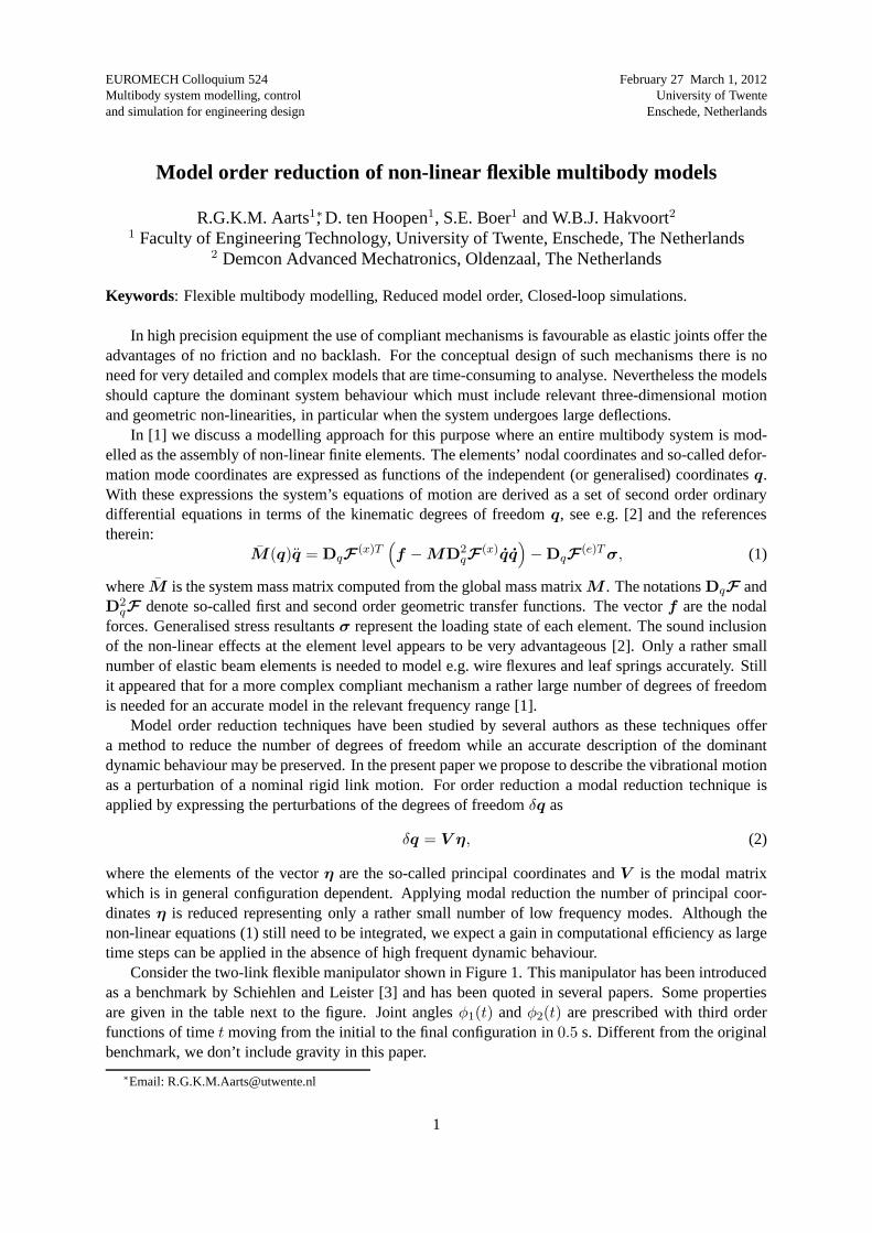

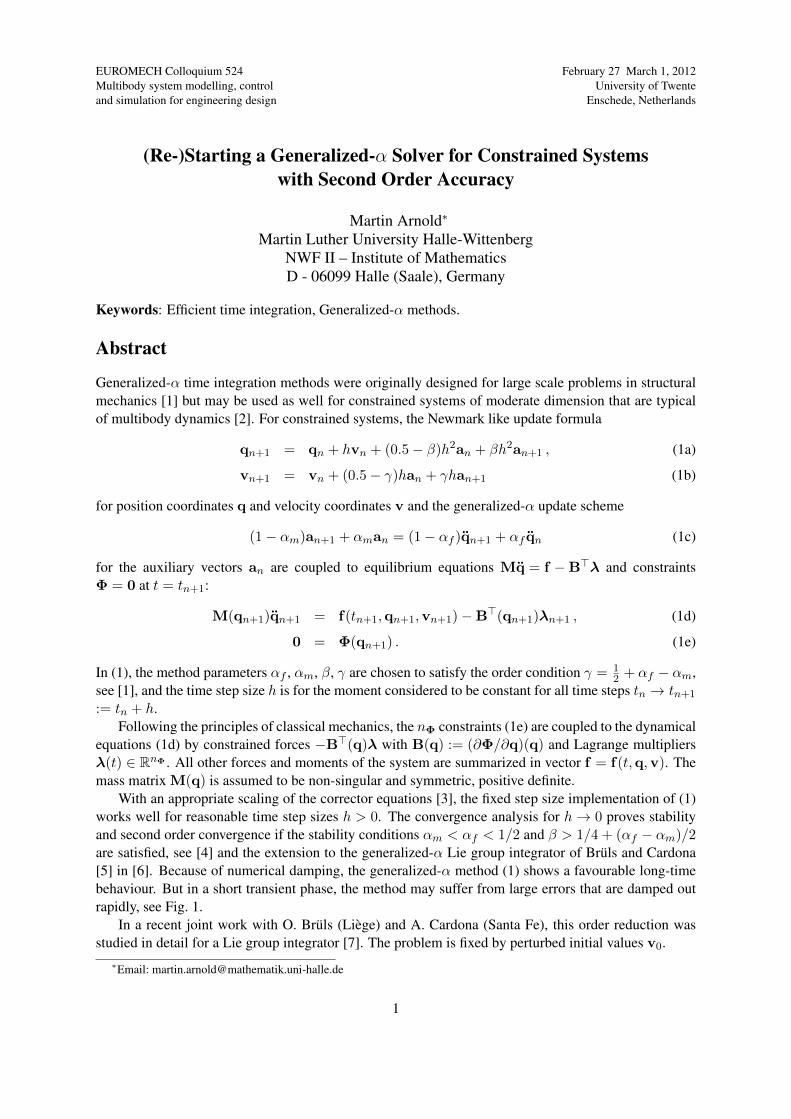


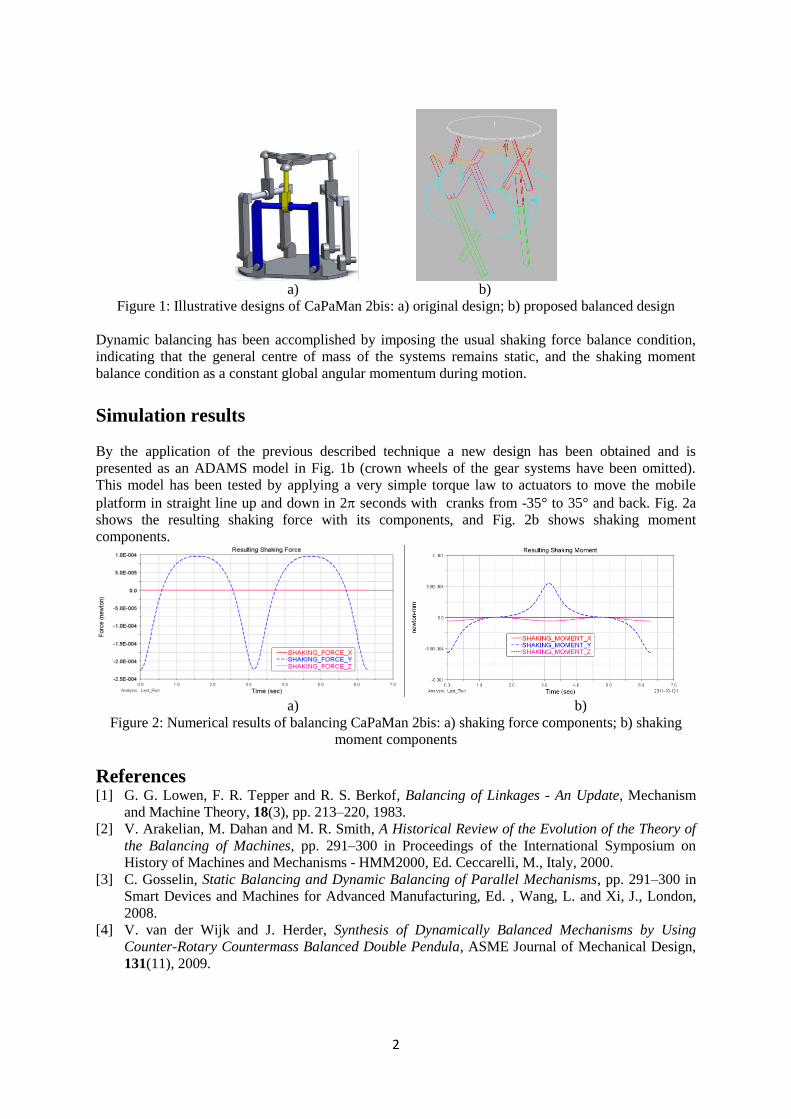


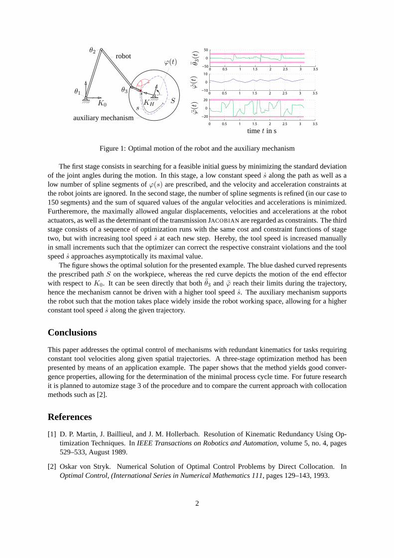


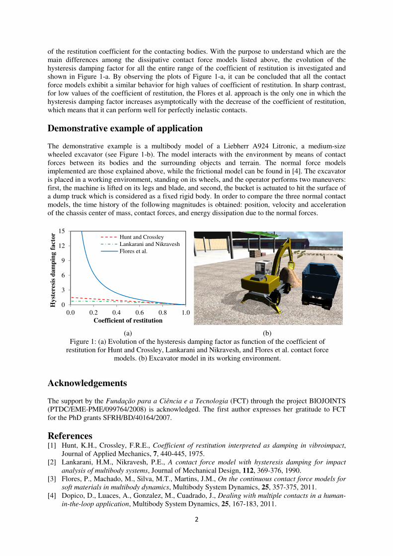

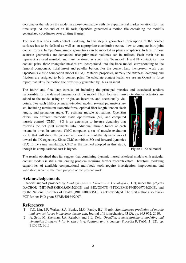


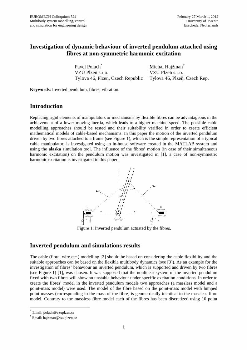


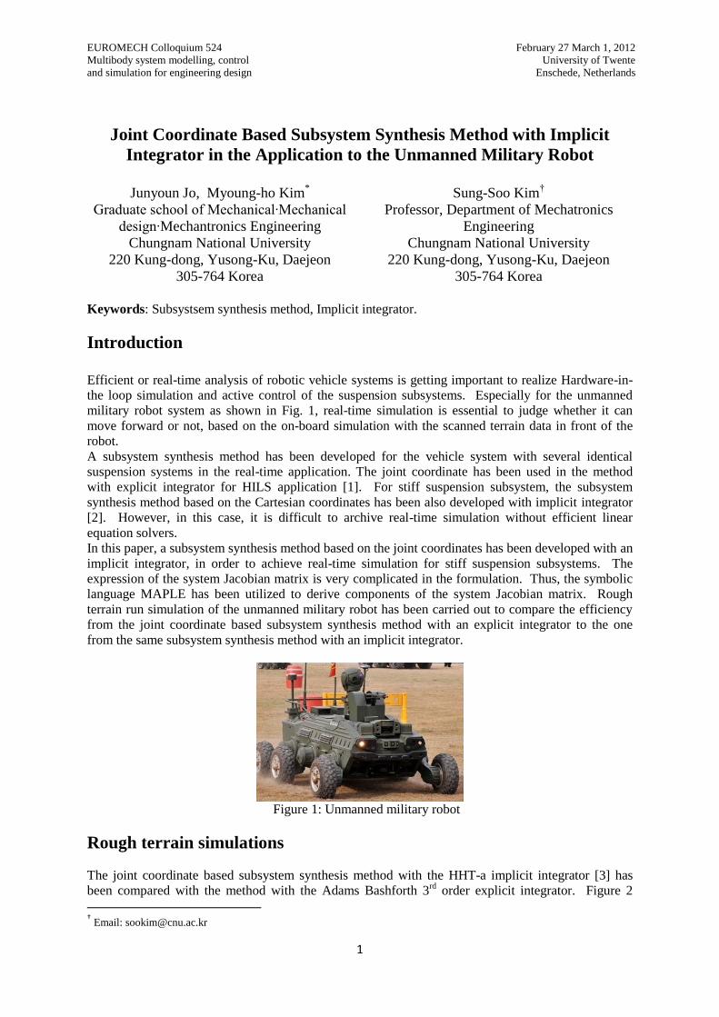


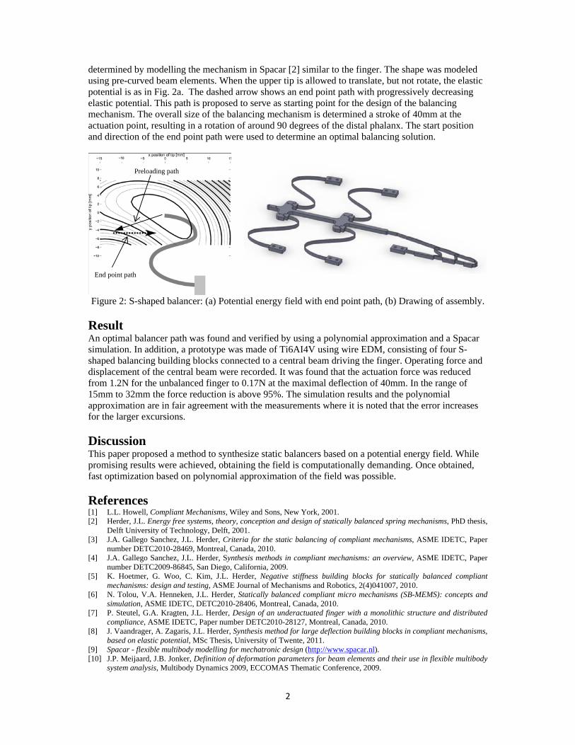


![Position-Dependent Multibody Dynamic Modeling of …home.iitk.ac.in/~mlaw/Law_ASME_paper.pdf · flexible multibody dynamic analysis software [4,5]. These co-simulations are time](https://static.documents.pub/doc/80x56/5b5e74017f8b9af90c8bd660/position-dependent-multibody-dynamic-modeling-of-homeiitkacinmlawlawasmepaperpdf.jpg)


![Interactive simulation of one-dimensional flexible parts · interactive contact simulation [1] as well as a real-time multibody dynamics [2]. This software had to treat flexible](https://static.documents.pub/doc/80x56/5fdae0129730eb027b25f761/interactive-simulation-of-one-dimensional-iexible-parts-interactive-contact-simulation.jpg)


