156
Model Predictive Control of Wind Turbines Martin Klauco Kongens Lyngby 2012 IMM-MSc-2012-65

Model Predictive Control
of
Wind Turbines
Martin Klauco
Kongens Lyngby 2012
IMM-MSc-2012-65

Technical University of Denmark
Informatics and Mathematical Modelling
Building 321, DK-2800 Kongens Lyngby, Denmark
Phone +45 45253351, Fax +45 45882673
www.imm.dtu.dk IMM-MSc-2012-65
Summary
Wind turbines are the biggest part of the green energy industry. Increasinginterest of governments and private companies in this industry calls for contin-uing innovation in development, construction and operation. Great portion ofthe operational front lies in designing new and more efficient control strategies.
Control strategy has a significant impact on the wind turbine operation on manylevels. First and foremost, it is the electrical power production. Secondly, thecost of power production is directly effected by the controller. On the thirdcount, the lifetime of the turbine and its components is greatly effected by thecontroller and its performance.
One of control strategies, which can take into account, maximization of powerproduction, minimization of costs and minimization of physical stress is calledModel Predictive Control (MPC). In this thesis such control method is explored.Key principles of such control strategy is presented in this research, togetherwith performed simulations. It will be shown, that this method is suitable forwind turbine control, and that it is capable of dealing with all presented issues.

ii

Preface
This thesis was prepared at the department of Informatics and MathematicalModelling at the Technical University of Denmark in fulfilment of the require-ments for acquiring an M.Sc. degree in Electrical Engineering. My supervisorswere Niels Kjølstad Poulsen, Mahmood Mirzaei both from IMM DTU and HansHenrik Niemann from DTU Elektro.
This research deals with controlling and modelling issues of the wind turbines.Main attention was put on design two alternative MPC strategies. These MPCstrategies were then compared with baseline PID controller, which is currentlyrunning on the actual wind turbines.
Results of this research were presented at GRØN DYST conference held at DTUon June 22, 2012.
Lyngby, July 2012
Martin Klauco

iv

Acknowledgements
I would like to express my deepest gratitude to Niels, for giving me the op-portunity to be part of the research at IMM DTU. I would especially like tothank him for his continuous support and guidance. My thanks also goes toMahmood, with whom I spent countless hours consulting technical stuff andimplementation. Furthermore I would like to thank Henrik for his insight andideas during project development.

vi

Nomenclature
Acronyms
MPC Model Predictive ControlFMPC Frequency Weighted Model Predictive ControlRHC Receding Horizon ControlHAWT Horizontal Axis Wind TurbineWT0 Model of the Wind Turbine, considering only rotor
speed as a stateWT1 Model of the Wind Turbine, considering also tower for-
aft movement
Physical Quantities
R m rotor disc radiusρ kg.m−3 specific weight of the air (density)ωr rad.s−1 angular velocity of the rotorJ kg.m2 moment of inertiaP W powerm kg.s−1 mass flow of the air moving against rotor discFt N thrust force affecting the towerxt m tower displacementMt kg total mas of the HAWTDt N.m−1.s−1 tower dampening constantKt N.m−1 tower spring constant

viii
Notation related to Modelling and Control
x state vectory output vectorym output measurements vectoru control input vectord state disturbance vectorA state space system matrixB state space control matrixC state space output matrixD state space direct matrixEx state space state disturbance matrixEy state space output disturbance matrixL Estimator gain (Kalman filter gain)Gu,x Transfer function from input u to state x (or output y)Rc,d covariance matrix in continuous (discrete) timeH curvature matrix (quadratic programming)g first order coefficient vector (quadratic programming)nu,x,y number of inputs, states and outputs
"ˆ" denotes estimation of given variable" s " denotes steady state values of given variable" 0 " denotes linearization point" ∗ " denotes coordinates of maximum of the cp curve
Sets
Rn Vector of real numbersRn×m Matrix of real numbersS+ Symmetric positive definite matrixIn×m Identity matrixdiag(x1,..,n) diagonal matrix with diagonal entries x1, ..., xn
diag(M1, ..., Mn) block diagonal matrix with diagonal blocks M1, ..., Mn

ix

x Contents
Contents
Summary i
Preface iii
Acknowledgements v
Nomenclature vii
1 Introduction 1
1.1 Horizontal Axis Wind Turbine Overview . . . . . . . . . . . . . . 11.2 Survey of Wind Turbine Control . . . . . . . . . . . . . . . . . . 21.3 Model Predictive Control Overview . . . . . . . . . . . . . . . . . 31.4 Project overview . . . . . . . . . . . . . . . . . . . . . . . . . . . 4
2 Model of Wind Turbine 5
2.1 Model of the HAWT . . . . . . . . . . . . . . . . . . . . . . . . . 52.2 Wind speed model . . . . . . . . . . . . . . . . . . . . . . . . . . 92.3 Operational and Stationary Analysis . . . . . . . . . . . . . . . . 132.4 Linearization . . . . . . . . . . . . . . . . . . . . . . . . . . . . . 182.5 Step Responses . . . . . . . . . . . . . . . . . . . . . . . . . . . . 25
2.5.1 Partial Load Case . . . . . . . . . . . . . . . . . . . . . . 252.5.2 Full Load Case . . . . . . . . . . . . . . . . . . . . . . . . 30
2.6 Frequency Responses . . . . . . . . . . . . . . . . . . . . . . . . . 35
3 Wind Speed Estimation and Disturbance Modelling 41
3.1 Wind Speed Estimation . . . . . . . . . . . . . . . . . . . . . . . 413.2 Disturbance Modelling . . . . . . . . . . . . . . . . . . . . . . . . 42
xii CONTENTS
4 Model Predictive Control 454.1 Standard MPC . . . . . . . . . . . . . . . . . . . . . . . . . . . . 45
4.1.1 Unconstrained MPC . . . . . . . . . . . . . . . . . . . . . 474.1.2 Hard Constraints . . . . . . . . . . . . . . . . . . . . . . . 524.1.3 Soft Constraints . . . . . . . . . . . . . . . . . . . . . . . 53
4.2 Frequency Weighted MPC . . . . . . . . . . . . . . . . . . . . . 57
5 Model Predictive Control Design for HAWT 615.1 Main Design . . . . . . . . . . . . . . . . . . . . . . . . . . . . . . 61
5.1.1 Model Scaling . . . . . . . . . . . . . . . . . . . . . . . . . 625.1.2 Standard MPC . . . . . . . . . . . . . . . . . . . . . . . . 635.1.3 Frequency Weighted MPC . . . . . . . . . . . . . . . . . . 65
5.2 Operational Constraints . . . . . . . . . . . . . . . . . . . . . . . 695.3 Simulations . . . . . . . . . . . . . . . . . . . . . . . . . . . . . . 70
6 Full Load Simulations 736.1 Standard MPC . . . . . . . . . . . . . . . . . . . . . . . . . . . . 746.2 Frequency weighted MPC . . . . . . . . . . . . . . . . . . . . . . 80
6.2.1 Filters on control inputs . . . . . . . . . . . . . . . . . . . 806.2.2 Filters on rotational speed and power . . . . . . . . . . . 836.2.3 Filters on states related to tower movement . . . . . . . . 836.2.4 Final tuning . . . . . . . . . . . . . . . . . . . . . . . . . . 90
7 Partial Load Simulations 937.1 WT0 model . . . . . . . . . . . . . . . . . . . . . . . . . . . . . . 93
7.1.1 Simulations in R-I . . . . . . . . . . . . . . . . . . . . . . 937.1.2 Simulations in R-II . . . . . . . . . . . . . . . . . . . . . . 967.1.3 Simulations in R-III . . . . . . . . . . . . . . . . . . . . . 99
7.2 WT1 model . . . . . . . . . . . . . . . . . . . . . . . . . . . . . . 1017.2.1 Simulation between R-I and R-II . . . . . . . . . . . . . . 1017.2.2 Simulation between R-II and R-III . . . . . . . . . . . . . 1057.2.3 Simulation between R-III and R-IV . . . . . . . . . . . . 1087.2.4 Overall Simulation . . . . . . . . . . . . . . . . . . . . . . 112
8 Comparison of MPC Control with Baseline Controller 1158.1 Baseline Controller . . . . . . . . . . . . . . . . . . . . . . . . . . 1158.2 Simulations with baseline controller . . . . . . . . . . . . . . . . . 116
8.2.1 Full Load Simulations . . . . . . . . . . . . . . . . . . . . 1168.2.2 Partial Load Simulations . . . . . . . . . . . . . . . . . . 121
9 Conclusion & Perspectives 1259.1 Conclusion . . . . . . . . . . . . . . . . . . . . . . . . . . . . . . 125
9.1.1 Theory and Methods . . . . . . . . . . . . . . . . . . . . . 1259.1.2 Simulations and Results . . . . . . . . . . . . . . . . . . . 126

CONTENTS xiii
9.2 Perspectives . . . . . . . . . . . . . . . . . . . . . . . . . . . . . . 126
A System Parameters 129A.1 Physical Parameters of Wind Turbine . . . . . . . . . . . . . . . 129A.2 Calculated Matrices and Transfer Functions . . . . . . . . . . . . 129
B Detailed Frequency Responses 133
Bibliography 137

xiv CONTENTS
Chapter 1
Introduction
Every control strategy implemented on processes has two main objectives. En-sure maximum yield, and minimize the cost. Since this project deals with windturbine control, the objective is to maximize the power output, and minimizethe costs of achieving previously mentioned objective. In this case, we not onlywant to minimize the cost of control activity, but also minimize physical stressof the device itself, thus prolonging the life of the turbine.
One of the control method, which can fulfil those objective is called ModelPredictive Control (MPC).
1.1 Horizontal Axis Wind Turbine Overview
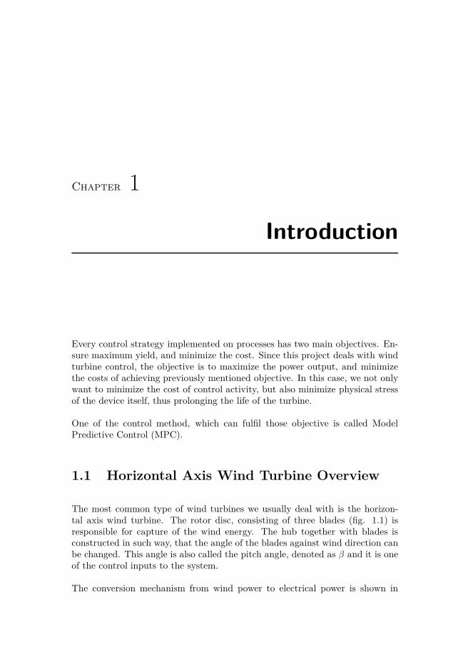
The most common type of wind turbines we usually deal with is the horizon-tal axis wind turbine. The rotor disc, consisting of three blades (fig. 1.1) isresponsible for capture of the wind energy. The hub together with blades isconstructed in such way, that the angle of the blades against wind direction canbe changed. This angle is also called the pitch angle, denoted as β and it is oneof the control inputs to the system.
The conversion mechanism from wind power to electrical power is shown in

2 Introduction
Figure 1.1: Horizontal Axis Wind Turbine (HAWT)
picture 1.2. The second control input to the system is the speed of the generator,or the generator torque - Tg. With these two control action, rotational speed ofthe rotor ωr and generated electrical power Pe can be controlled. We have tomention, that in case of HAWT, nacelle yaw angle is controlled as well, but it isassumed that direction of wind speed does not change, so it is committed fromcontrol design in this project.
Power
Rotor
trainDrive
Generator
Generatorspeed
Rotorspeed
Pitchangle
Powerdemand
speedWind
Actuator demandPitch
Controller
α
GridPower
electronics
Figure 1.2: Generator with controller (Xin, 1994)
1.2 Survey of Wind Turbine Control
Standard and most common approach, that has been used on controlling thewind turbines all over the world are single-input-single-output (SISO) loops

1.3 Model Predictive Control Overview 3
(Jonkman et al., 2009). So far this control approach has proven to have satis-factory performance. This control strategy si more than suitable to handle theprimary control objective, specifically produce maximum power (Laks et al.,2009).
However, when the wind turbine industry is on the rise more advanced controlstrategies are needed. The main control objective remain the power production,but secondary tasks arise, e.g. decreasing structural fatigue, thus prolonging thelifetime of the turbine and its components. In order to fulfil these objectives,multiple-input-multiple-output (MIMO) methods must be used. For such pur-pose robust model predictive control has been proposed (Mirzaei et al., 2012b).Another approach presented by (Østergaard et al., 2008) propose linear param-eter varying control strategy, as an advanced gain scheduling method in orderto control wind turbine in entire considered wind speed interval. These meth-ods are based on linear models. It will be shown, that system dynamics changewith increasing wind speed. This means, that estimation or measurement of thewind speed is required, based on which LTI models. Also MPC control or LQcontrol are based on state feedback, so state estimator is required when usingsuch controllers.
Above presented methods consider collective blade pitch control action. Sincethe wind speed is not constant throughout the rotor disc, individual blade pitchcontrol has been proposed (Bossanyi, 2003). In paper presented by (Mirzaeiet al., 2012a) is proposed individual blade pitch robust model predictive con-troller together with wind speed measurements over the prediction horizon. Thisproves to have significant advantages when harsh wind speed conditions occursi.e. wind shears.
1.3 Model Predictive Control Overview
Model predictive control (MPC) is an advanced MIMO optimal control strat-egy. The basic principle of MPC lies in predicting the future states of the plants,then formulating an cost function which reflects control objective and imposingadditional constraints on inputs, states or outputs. MPC problem is often for-mulated as a quadratic programming problem (Boyd and Vandenberghe, 2009;Nocedal and Wright, 1999), which is solved at each sampling instance to obtainoptimal control inputs.
MPC has become one the most used process control tools mainly in chemicalindustry like distillation columns (Ahmad and Wahib, 2007), but also oil re-fineries and such (Nikolaou, 2001). Main advantage of it in such applications

4 Introduction
is the way of handling huge time delays. Advantages of MPC are also used inelectrical power industry (Larsson, 2004), smart grids optimization and design(Bendtsen et al., 2010) etc. Theory behind Model Predictive Control is furtherdiscussed in chapter 4.
1.4 Project overview
Every process control design must begin with deriving mathematical model ofthe process. In our case it is the Wind-Turbine. Once the mathematical modelis formulated, MPC design is explained. In this project we will focus on twoapproaches of controlling the HAWT.
In the controller design we will focus on the MPC design. Two approaches ofMPC control will be explained. First, the most common one, where the tuningparameters of the controller are weighting matrices (Camacho and Bordons,2007). In second part of MPC design we will focus on frequency weightedMPC control design. Advantages and disadvantages of MPC strategies will beexplained. Furthermore Kalman filtering for state and disturbance estimationis going to be discussed (Kalman, 1960; Pannocchia and Rawlings, 2003).
In order to demonstrate the performance of the model predictive control strat-egy, detailed deterministic simulations are shown along with long time stochasticsimulations. Performance of standard MPC is then compared with the frequencyweighted MPC design. The effects of the frequency weights (filters) are going tobe explained as well. Furthermore these two MPC strategies will be comparedwith currently implemented PID controllers (Jonkman et al., 2009; J. Jonkmanand Bir, 2007); it will be shown, that MPC design has stabilized the poweroutput of the HAWT, and that it minimizes the physical stress to the turbine.

Chapter 2
Model of Wind Turbine
2.1 Model of the HAWT
Kinetic energy of the wind is the driving force of the power generation in wind-turbine. The following formula shows hot to calculate kinetic energy of an object
E =12
mv2 (2.1)
where m is mass and v is speed of object and E is the kinetic energy. Themechanical power is defined as a first derivative of energy with respect to time:
P =dE
dt(2.2)
Since the speed is considered constant, we can combine equations 2.1 and 2.2together
P =12
dm
dtv2 =
12
mv2 (2.3)
where m is considered as mass flow. In case of HAWT, the mass flow is the airmoving against rotor disc, therefore we can write:
m = πR2ρv (2.4)

6 Model of Wind Turbine
where ρ is the density of the air, R is the length of the blades and v is the speedof the wind. The equation 2.5 shows how to calculate the power stored in thewind, which is moving against the wind turbine (Xin et al., 1997; Burton et al.,2001).
Pw =12
mv2 =12
ρπR2v3 (2.5)
It is only natural, that the wind turbine cannot extract 100% of the powerstored in the wind. The coefficient, which determines how much power is actu-ally converted into electrical energy is called power extraction coefficient or CP
value. This value is function of pitch angle and tip speed ratio. The maximummechanical power, available in the wind speed is expressed in equation 2.6.
Pr =12
ρπR2v3Cp(λ, β) (2.6)
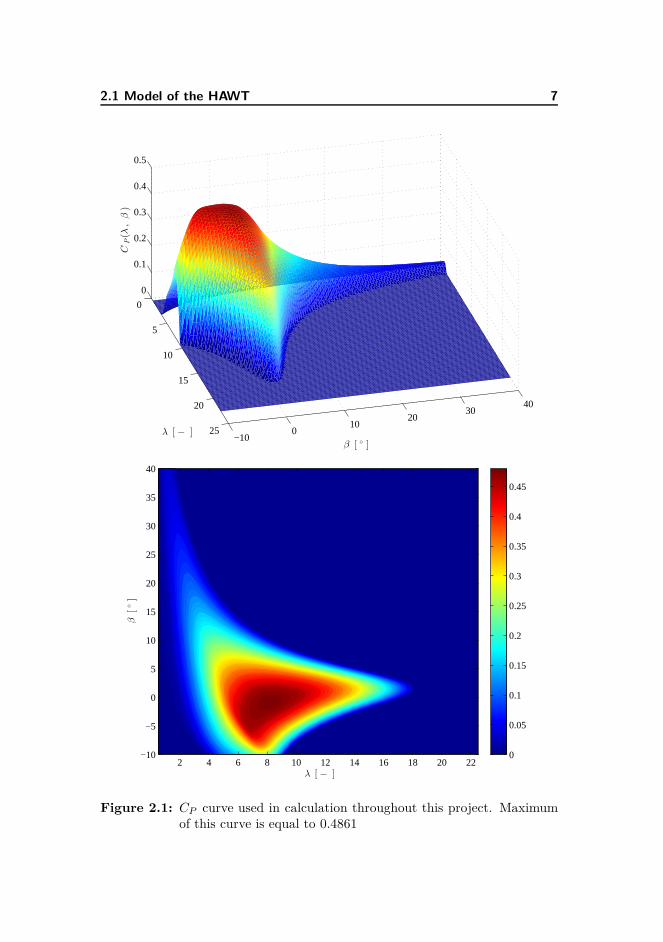
Power coefficient CP (λ, β) is a function of tip speed ratio (TSR) λ, (eq. 2.7)and pitch β. The cp curve is displayed on the figure 2.1.
λ =Rωr
v(2.7)
The rotation movement of the rotor is given by formula 2.8:
Jdωr
dt= Qr − NgTg (2.8)
Where J is the inertia of the system, Qr is aerodynamic torque, Ng is gear ratioand Tg is the generator torque. Aero dynamic torque is given as ratio betweenmechanical power, and rotational speed ωr (eq. 2.9).
Qr =Pr
ωr
(2.9)
In similar fashion like Cp(λ, β) curve, is defined Ct(λ, β) curve (fig. 2.2). Basedon ct coefficient we can calculate the thrust force Ft imposed by the wind onthe tower (eq. 2.10).
Thrust force:Ft =
12
πρR2v2ct(λ, β) (2.10)
2.1 Model of the HAWT 7
0
5
10
15
20
25−10
010
2030
40
0
0.1
0.2
0.3
0.4
0.5
β [ ◦ ]
λ [ − ]
CP(λ
,β)
λ [ − ]
β[◦]
2 4 6 8 10 12 14 16 18 20 22−10
−5
0
5
10
15
20
25
30
35
40
0
0.05
0.1
0.15
0.2
0.25
0.3
0.35
0.4
0.45
Figure 2.1: CP curve used in calculation throughout this project. Maximumof this curve is equal to 0.4861

8 Model of Wind Turbine
0
5
10
15
20
25
−10
0
10
20
30
40
−10
−5
0
5
10
λ [ − ]
β [ ◦ ]
CT(λ
,β)
λ [ − ]
β[◦]
2 4 6 8 10 12 14 16 18 20 22−10
−5
0
5
10
15
20
25
30
35
40
−6
−4
−2
0
2
4
6
Figure 2.2: Thrust coefficient
2.2 Wind speed model 9
Tower for-aft movement can be represented by second order system (Hansen,2008). Equation 2.11 shows the relation between thrust force, tower speedof displacement xt and tower displacement xt. Mass constant Mt, structuraldamping factor Dt and spring constant Kt can be found in (Henriksen, 2007).
Ft = Mtxt + Dtxt + Ktxt (2.11)
Stationary value of tower displacement is calculated:
xt,0 =Ft
Kt
(2.12)
2.2 Wind speed model
Effective wind speed is approximated by second order transfer function 2.13.Where parameters k, p1, p2 are functions of mean wind speed (Xin et al., 1997;Henriksen, 2007). Values for these parameters can be found in figure 2.3.
vt =k
(p1s + 1)(p2s + 1)et; et ∈ Niid(0, 1) (2.13)
A substitution 2.14 has been introduced in order to obtain continuous statespace model of the wind speed, this mode is expressed in 2.15.
x1 = vx2 = v
(2.14)
[
x1
x2
]
=[
0 1a1 a2
] [
x1
x2
]
+[
0b1
]
et (2.15)
yielding:
x = Acx + Bcet (2.16)
As far, as we are only interested in wind speed itself, not wind acceleration,output C matrix for this state space model will be:
C = [1 0] (2.17)

10 Model of Wind Turbine
5 10 15 20 25 30
5
6
7
8
9
10
11
12
13
vm [m/s]
k[−
]
(a) Gain
5 10 15 20 25 30
1
2
3
4
5
6
vm [m/s]
σ2[−
]
(b) Noise Variance
5 10 15 20 25 30
20
40
60
80
100
120
140
vm [m/s]
p1[s]
(c) Time constatnt p1
5 10 15 20 25 30
1
1.5
2
2.5
3
3.5
4
vm [m/s]
p2[s]
(d) Time constatnt p2
Figure 2.3: Wind speed model parameters for transfer function defined inequation 2.13

2.2 Wind speed model 11
Coefficients in Ac matrix can be simply calculated from transfer function pre-sented earlier (eq. 2.13).
a1 = −1
p1p2a2 = −
p1 + p2
p1p2b1 =
k
p1p2(2.18)
Covariance matrix in continuous time for wind speed model is given in equation2.19, where the intensity I is equal to 1.
Rc = BIBT (2.19)
In order to better understand how the variance of the wind speed changes withincreasing mean wind speed, stationary distribution of the output of the statespace model is calculated. Using Lyapunov equation in continuous time (eq.2.20) we calculate the stationary distribution of the states X . The variance ofthe wind speed can be then calculated using formula 2.21. Result is shown infigure 2.3(b).
0 = AcX + XATc + Rc (2.20)
σ2 = CXCT (2.21)
Since discrete time simulations has been performed, continuous model must bediscretized. The target discrete time state space model is shown in 2.22. Inwhich x is the state vector. The variable vk is the discrete time value of theeffective wind speed and vm is the mean wind speed.
xk+1 = Adxk + Rdek (2.22a)
vk = Cxk + vm (2.22b)
In our case covariance matrix Rc must be also discretized. For calculationwe used procedure thoroughly described in (Brown and Hwang, 1997; Åström,1970). For an illustration this procedure will be shortly explained. First matrixF is constructed (eq. 2.23), then matrix G is calculated using formula 2.24.Note, that when using Matlab for this calculation, matrix exponential expm
must be used. In order to obtain the discrete time covariance matrix and discretetime system matrix, matrix G is split into sub-matrices like suggested in 2.24

12 Model of Wind Turbine
0 20 40 60 80 100 1204
6
8
10
12
14
16
18
20
Time [s]
v[m
/s]
Wind speed profile
vm = 5 m/svm = 10 m/svm = 15 m/s
Figure 2.4: Generated wind profile for different mean wind speeds
and 2.25. Equation 2.26 shows the covariance matrix in discrete time. Samplingtime τs was set to 0.1 s. This sampling time was also used on discretization ofstate space models.
F =[
−A Rc
0 AT
]
(2.23)
G = eF τs =[
M11 M12
0 M22
]
(2.24)
M12 = A−1d Rd
M22 = ATd
(2.25)
Rd = MT22M12 (2.26)
2.3 Operational and Stationary Analysis 13
Using the discrete time state space model, we can generate the wind speed profilefor discrete time simulations. On figure 2.4 are shown profiles for different meanwind speeds. In order to demonstrate the difference in the variance, same set ofrandom numbers were used.
More data about wind turbines standards and wind speed definitions can befound in (IEC-CDV, 2004).
2.3 Operational and Stationary Analysis
Horizontal Axis Wind Turbine operates in 4 operational modes. These oper-ational region are defined by rotational speed ωr, generated power Pe and bywind speed v. Values of rotational speed can be found on figure 2.5. Figure 2.6shows the stationary value for power output.
Region 1 (R-I) - Low Region: Angular velocity of the rotor is kept at itsminimum value, ωr,1 = 6.9 rpm. In this region, power is maximized. In orderto do that pitch values are found for given TSR, so the value of cp is maximumpossible. The wind speed interval for this region is v ∈ < 3, 5.6 > m/s.
Region 2 (R-II) - Mid Region: In this region the maximum of the cp(λ, β)curve is reached. Velocity of the rotor rise linearly with the wind speed (eq.2.27). Power is again maximized in this region. Pitch values and TSR valuesare kept constant. λ⋆ and β⋆ denotes the coordinates of the maximum of the cp
curve. The wind speed interval for this region is v ∈ < 5.6, 10 > m/s
ωr,2 =λ⋆R
v(2.27)
Region 3 (R-III ) - High Region: Rotor speed is kept at its nominal valueωr,3 = 12.1 [rpm]. Also in this region power is maximized. The pitch values arefound, so the values of power coefficient cp is maximum possible, given λ. Thewind speed interval for this region is v ∈ < 10, 11.2 >
Region 4 (R-IV) - Top Region: Both power output and angular velocity iskept at their respective nominal values. cp values are calculated from formula2.28. The wind speed interval for this region is v ∈ < 11.2, 25 > m/s
cp(λ, β) =2Pnom
ρπR2v3(2.28)

14 Model of Wind Turbine
Definition of the operational modes of the HAWT is resulting in stationary val-ues of individual quantities linked to HAWT, like cp values (fig. 2.7). Followingby figures which display stationary values of pitch β and TSR λ with respect towind speed (figures 2.8 and 2.9).
3 5.6 10 11.2 256
6.9
9.5
12.113
vm [m/s]
ωr[rpm]
Figure 2.5: Steady state values of angular velocity of the rotor (ωr)
3 5.6 10 11.2 250
1
2
3
4
5
vm [m/s]
Pr[M
W]
Figure 2.6: Mechanical power (Pr) generated by the rotor

2.3 Operational and Stationary Analysis 15
3 5.6 10 11.2 250
0.1
0.2
0.3
0.4
0.5
vm [m/s]
c p(λ,β
)[-]
Figure 2.7: Steady state values of power extraction coefficient (cp)
3 5.6 10 11.2 25−10
0
10
20
30
vm [m/s]
β[◦]
Figure 2.8: Steady state values of pitch (β)
3 5.6 10 11.2 250
5
10
15
20
vm [m/s]
λ[-]
Figure 2.9: Steady state values of TSR (λ)

16 Model of Wind Turbine
2 4 6 8 10 12 14 16 18 20 22−10
−5
0
5
10
15
20
25
30
35
40
λ [-]
β[deg]
cp(λ,β)cp,0cp,max
0.05
0.1
0.15
0.2
0.25
0.3
0.35
0.4
0.45
Figure 2.10: Contour plot of cp(λ, β) curve
Figure 2.10 shows contour plot of the Cp curve, with the stationary values of theTSR, and pitch. Stationary values of cp(λ, beta) are denoted as c0
p. This figureis crucial for understating the definitions of operational modes. In low windspeeds, TSR is high, and pitch values are found so in order to get maximumcp value (first three regions). In second region, the pitch is kept constant, themaximum of the cp. However in the top region, when the objective is to controlthe power, the pitch is calculated so generated power is equal to nominal power.
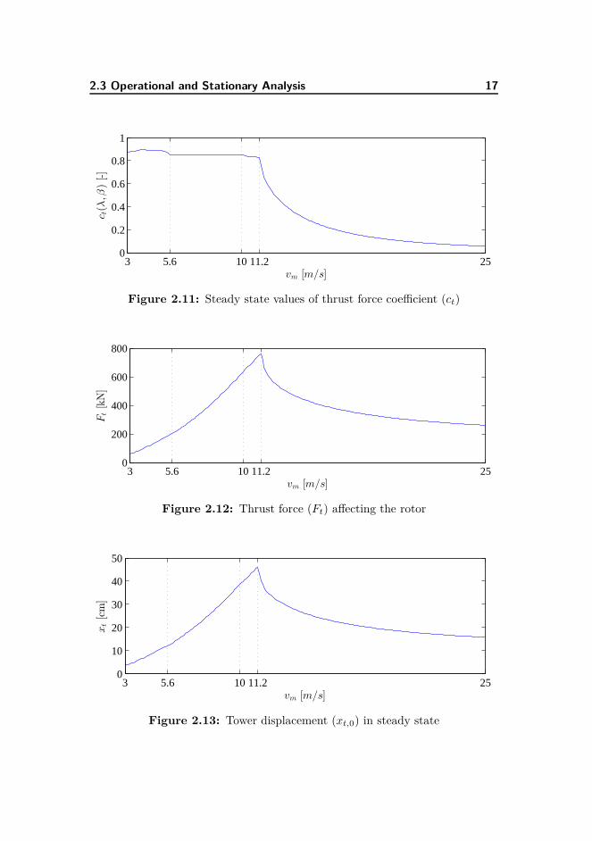
Once we calculated these basic quantities, which describes behaviour of the rotorangular velocity at every wind speed, we can calculate values of ct curve (fig.2.11), and thrust force Ft (fig. 2.12) as a function of wind speed. Stationaryvalue of tower displacement xt as a function of wind speed is shown on figure2.13.
2.3 Operational and Stationary Analysis 17
3 5.6 10 11.2 250
0.2
0.4
0.6
0.8
1
vm [m/s]
c t(λ,β
)[-]
Figure 2.11: Steady state values of thrust force coefficient (ct)
3 5.6 10 11.2 250
200
400
600
800
vm [m/s]
Ft[kN]
Figure 2.12: Thrust force (Ft) affecting the rotor
3 5.6 10 11.2 250
10
20
30
40
50
vm [m/s]
xt[cm]
Figure 2.13: Tower displacement (xt,0) in steady state
18 Model of Wind Turbine
2.4 Linearization
In order to design linear model, on which is based the MPC controller, properderivatives of physical quantities must be found. Model considered in thisproject is a third order system (eq. 2.29) with two control inputs (2.30). Windspeed is considered as a disturbance.
x =
ωr
xt
xt
(2.29)
u =[
βTg
]
(2.30)
Differential equations that describes the system behaviour are:
Jωr = Qr − NgTg (2.31a)
Ft = Mtxt + Dtxt + Ktxt (2.31b)
Once the tower for-aft movement is considered as a part of the model (Hansen,2008), then we also have to consider relative wind speed vr (eq. 2.32). It isobvious, that if the steady state point is reached, relative wind speed is equalto actual wind speed. The relative wind speed will be the operating point onwhich is based the linearization of the states related to the tower movement.
vr = v − xt (2.32a)
v = vr + xt (2.32b)
Linearization of non-linear system presented in equation 2.31 takes place usingvery well-known first order Taylor series expansion. Partial derivatives respec-tive functions in eq. 2.31 given all states, control and disturbance variables mustbe found.
First we will introduce derivatives of the aerodynamic torque with respect toconsidered variables.
∂Qr
∂ωr
∣
∣
∣
∣
ωr0
=1
ωr0
∂Pr
∂ωr
∣
∣
∣
∣
ωr0
−Pr0
ω2r0
(2.33)

2.4 Linearization 19
∂Qr
∂β
∣
∣
∣
∣
β0
=1
ωr0
∂Pr
∂β
∣
∣
∣
∣
β0
(2.34)
∂Qr
∂β
∣
∣
∣
∣
v0
=1
ωr0
∂Pr
∂v
∣
∣
∣
∣
v0
(2.35)
Then we further continue with the respective derivatives of the mechanical powerPr.
∂Pr
∂ωr
∣
∣
∣
∣
ωr0
=12
ρπR2v3 ∂cp(λ, β)∂λ
∣
∣
∣
∣
λ0
·∂λ
∂ωr
∣
∣
∣
∣
ωr0
(2.36)
∂Pr
∂β
∣
∣
∣
∣
β0
=12
ρπR2v3 ∂cp(λ, β)∂β
∣
∣
∣
∣
β0
(2.37)
∂Pr
∂v
∣
∣
∣
∣
v0
=12
ρπR2
(
3v20cp(λ0, β0) + v3 ∂cp(λ, β)
∂λ
∣
∣
∣
∣
λ0
·∂λ
∂v
∣
∣
∣
∣
v0
)
(2.38)
Since the xt is considered as a state variable, derivatives of Qr and Ft withrespect to xt must be calculated as well. Understanding the relation presentedin equation 2.32, following expression can be written:
∂Pr
∂xt,0
∣
∣
∣
∣
xt,0
=∂Pr
∂v
∣
∣
∣
∣
v0
(2.39)
Respective partial derivatives of TSR:
∂λ
∂ωr
=R
v(2.40)
∂λ
∂v= −
Rωr
v2(2.41)
Derivatives of CP with respect to λ and β (eq: 2.42) must be found numericallyusing various interpolation methods. Values of these derivatives as a functionof wind speed can be seen on figures 2.14 and 2.15.

20 Model of Wind Turbine
3 5.6 10 11.2 25−0.04
−0.03
−0.02
−0.01
0
0.01
vm [m/s]
∂c p ∂β
Figure 2.14: Values of partial derivative of Cp with respect to β
3 5.6 10 11.2 25−0.1
−0.05
0
0.05
0.1
vm [m/s]
∂c p ∂λ
Figure 2.15: Values of partial derivative of Cp with respect to λ
∂cp(λ, β)∂β
∣
∣
∣
∣
β0
(2.42a)
∂cp(λ, β)∂λ
∣
∣
∣
∣
λ0
(2.42b)
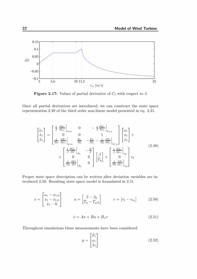
Model of the tower for-aft movement was made linear, so we can easily writestate space representation (eq. 2.43) of that differential equation (eq. 2.31b).
[
xt
xt
]
=[
0 1− Kt
Mt− Dt
Mt
] [
xt
xt
]
+[
01
Mt
]
Ft (2.43)
2.4 Linearization 21
3 5.6 10 11.2 25−0.2
−0.15
−0.1
−0.05
0
vm [m/s]
∂c t
∂β
Figure 2.16: Values of partial derivative of Ct with respect to β
Next partial derivatives of thrust force Ft are expressed:
∂Ft
∂ωr
∣
∣
∣
∣
ωr,0
=12
πρR2v2 ∂ct(λ, β)∂λ0
∣
∣
∣
∣
λ0
∂λ
∂ωr
∣
∣
∣
∣
ωr,0
(2.44)
∂Ft
∂β
∣
∣
∣
∣
β0
=12
πρR2v2 ∂ct(λ, β)∂β0
∣
∣
∣
∣
β0
(2.45)
∂Ft
∂v
∣
∣
∣
∣
v0
=12
πρR2
(
2vc0t (λ, β) + v2 ∂ct(λ, β)
∂λ0
∣
∣
∣
∣
λ0
∂λ
∂v
∣
∣
∣
∣
v0
)
(2.46)
∂Ft
∂xt
∣
∣
∣
∣
xt,0
=∂Ft
∂v
∣
∣
∣
∣
v0
(2.47)
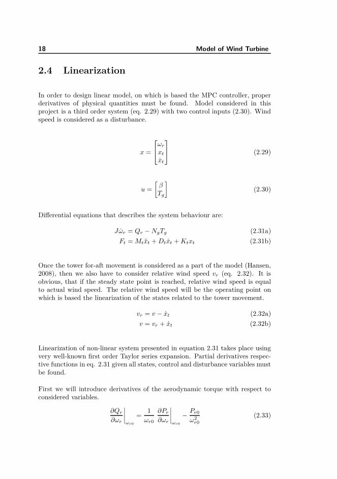
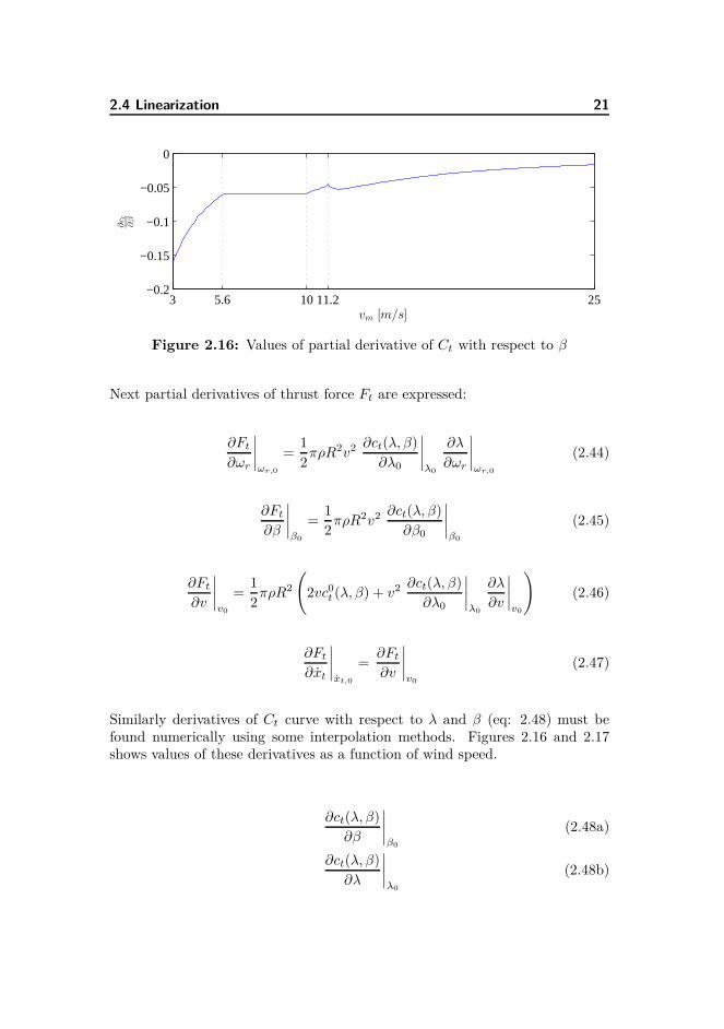
Similarly derivatives of Ct curve with respect to λ and β (eq: 2.48) must befound numerically using some interpolation methods. Figures 2.16 and 2.17shows values of these derivatives as a function of wind speed.
∂ct(λ, β)∂β
∣
∣
∣
∣
β0
(2.48a)
∂ct(λ, β)∂λ
∣
∣
∣
∣
λ0
(2.48b)
22 Model of Wind Turbine
3 5.6 10 11.2 25−0.1
−0.05
0
0.05
0.1
0.15
vm [m/s]
∂c t ∂λ
Figure 2.17: Values of partial derivative of Ct with respect to λ
Once all partial derivatives are introduced, we can construct the state spacerepresentation 2.49 of the third order non-linear model presented in eq. 2.31.
ωr
xt
xt
=
1J
∂Qr
∂ωr
∣
∣
∣
ωr0
0 − 1J
∂Qr
∂xt
∣
∣
∣
xt,0
0 0 11
Mt
∂Fr
∂ωr
∣
∣
∣
ωr0
Kt
Mt− Dt
Mt− 1
Mt
∂Ft
∂xt
∣
∣
∣
xt,0
ωr
xt
xt
+
+
1J
∂Qr
∂β
∣
∣
∣
β0
− NJ
0 01
Mt
∂Ft
∂β
∣
∣
∣
β0
0
[
βTg
]
+
1J
∂Qr
∂vr
∣
∣
∣
v0
01
Mt
∂Ft
∂vr
∣
∣
∣
v0
vt
(2.49)
Proper state space description can be written after deviation variables are in-troduced 2.50. Resulting state space model is formulated in 2.51
x =
ωr − ωr,0
xt − xt,0
xt − 0
u =[
β − β0
Tg − Tg,0
]
v =[
vt − vm
]
(2.50)
x = Ax + Bu + Bvv (2.51)
Throughout simulations these measurements have been considered:
y =
Pe
ωr
xt
(2.52)
2.4 Linearization 23
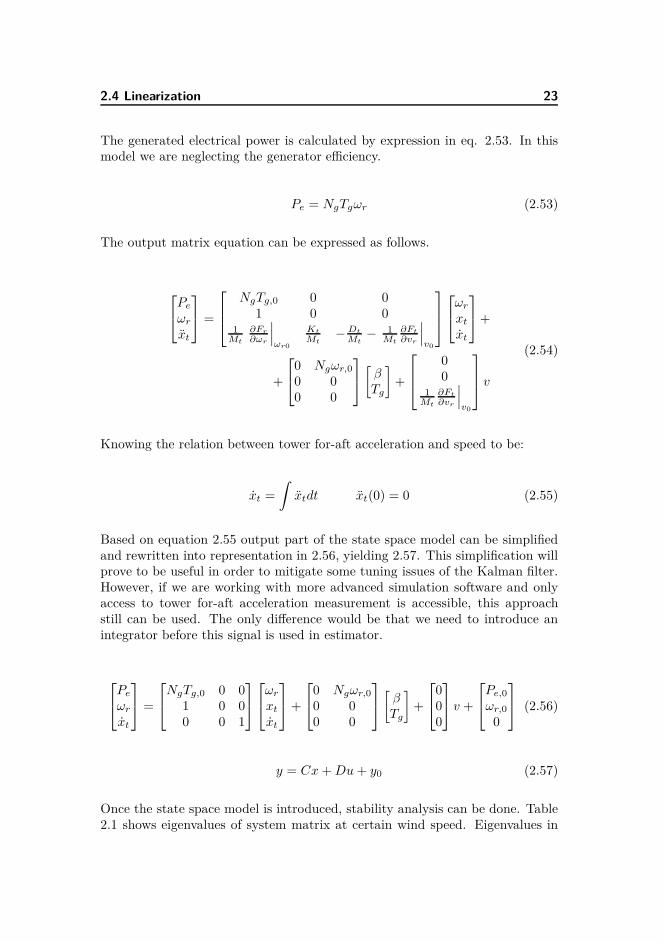
The generated electrical power is calculated by expression in eq. 2.53. In thismodel we are neglecting the generator efficiency.
Pe = NgTgωr (2.53)
The output matrix equation can be expressed as follows.
Pe
ωr
xt
=
NgTg,0 0 01 0 0
1Mt
∂Fr
∂ωr
∣
∣
∣
ωr0
Kt
Mt− Dt
Mt− 1
Mt
∂Ft
∂vr
∣
∣
∣
v0
ωr
xt
xt
+
+
0 Ngωr,0
0 00 0
[
βTg
]
+
00
1Mt
∂Ft
∂vr
∣
∣
∣
v0
v
(2.54)
Knowing the relation between tower for-aft acceleration and speed to be:
xt =∫
xtdt xt(0) = 0 (2.55)
Based on equation 2.55 output part of the state space model can be simplifiedand rewritten into representation in 2.56, yielding 2.57. This simplification willprove to be useful in order to mitigate some tuning issues of the Kalman filter.However, if we are working with more advanced simulation software and onlyaccess to tower for-aft acceleration measurement is accessible, this approachstill can be used. The only difference would be that we need to introduce anintegrator before this signal is used in estimator.
Pe
ωr
xt
=
NgTg,0 0 01 0 00 0 1
ωr
xt
xt
+
0 Ngωr,0
0 00 0
[
βTg
]
+
000
v +
Pe,0
ωr,0
0
(2.56)
y = Cx + Du + y0 (2.57)
Once the state space model is introduced, stability analysis can be done. Table2.1 shows eigenvalues of system matrix at certain wind speed. Eigenvalues in

24 Model of Wind Turbine
C-Time and D-Time are presented. Sampling frequency has been chosen asfs = 10 Hz. Table shows eigenvalue for rotational speed state denoted as λωr
,and eigenvalues for tower for-aft movement states denoted as λt.
Notice decreasing values of λωrwith increasing wind speed (in both C-Time
and D-Time). The eigenvalues related to tower movement are rising up to the11 m/s, and then decreasing (C-Time). This is consistent with calculation ofthrust force Ft, which is increasing up tp the critical wind speed (11.2 m/s) andthen decreasing (fig. 2.12).
Table 2.1: Eigenvalues
C-Time D-Timewind speed λωr
λt λωrλt
3 −0.0179 −0.0683 ± 1.9772i 0.9982 0.9738 ± 0.1951i5 −0.0269 −0.0789 ± 1.9776i 0.9973 0.9728 ± 0.1949i7 −0.0349 −0.0922 ± 1.9784i 0.9965 0.9715 ± 0.1947i9 −0.0463 −0.1118 ± 1.9788i 0.9954 0.9696 ± 0.1944i11 −0.0574 −0.1156 ± 1.9823i 0.9943 0.9691 ± 0.1947i13 −0.0795 −0.1122 ± 1.9750i 0.9921 0.9696 ± 0.1940i15 −0.1368 −0.1109 ± 1.9713i 0.9864 0.9698 ± 0.1937i17 −0.2039 −0.1098 ± 1.9676i 0.9798 0.9700 ± 0.1934i19 −0.2639 −0.1087 ± 1.9642i 0.9740 0.9702 ± 0.1930i21 −0.3325 −0.1076 ± 1.9605i 0.9673 0.9703 ± 0.1927i23 −0.4102 −0.1056 ± 1.9570i 0.9598 0.9706 ± 0.1924i25 −0.4806 −0.1032 ± 1.9540i 0.9531 0.9709 ± 0.1922i
2.5 Step Responses 25
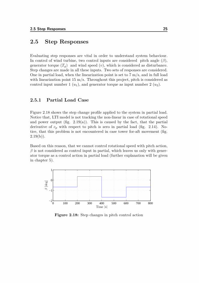
2.5 Step Responses
Evaluating step responses are vital in order to understand system behaviour.In control of wind turbine, two control inputs are considered pitch angle (β),generator torque (Tg) and wind speed (v), which is considered as disturbance.Step changes are made in all these inputs. Two sets of responses are considered.One in partial load, when the linearization point is set to 7 m/s, and in full loadwith linearization point 15 m/s. Throughout this project, pitch is considered ascontrol input number 1 (u1), and generator torque as input number 2 (u2).
2.5.1 Partial Load Case
Figure 2.18 shows the step change profile applied to the system in partial load.Notice that, LTI model is not tracking the non-linear in case of rotational speedand power output (fig. 2.19(a)). This is caused by the fact, that the partialderivative of cp with respect to pitch is zero in partial load (fig. 2.14). No-tice, that this problem is not encountered in case tower for-aft movement (fig.2.19(b)).
Based on this reason, that we cannot control rotational speed with pitch action,β is not considered as control input in partial, which leaves us only with gener-ator torque as a control action in partial load (further explanation will be givenin chapter 5).
0 100 200 300 400 500 600 700 800−2
−1
0
1
β[deg]
Time [s]
Figure 2.18: Step changes in pitch control action

26 Model of Wind Turbine
0 100 200 300 400 500 600 700 8008.4
8.45
8.5
8.55
8.6
ωr[rpm]
Non−linearLTI
0 100 200 300 400 500 600 700 8001.23
1.235
1.24
1.245
1.25
1.255x 10
6
Pe[W
]
Time [s]
(a) Measurements - Pe and ωr
0 100 200 300 400 500 600 700 8000.16
0.18
0.2
0.22
0.24
xt[m
]
Non−linearLTI
0 100 200 300 400 500 600 700 800−0.05
0
0.05
xt[m
/s]
Time [s]
(b) Tower displacement xt and speed of displacement xt
Figure 2.19: Response to change in pitch (β) control input (fig. 2.18)

2.5 Step Responses 27
When made step changes in generator torque input (2.20) or wind speed(2.21),LTI model and non-linear track themselves within acceptable margin. Noticethe effect of the generator torque effect on electrical power (fig. 2.22(a)). This iscaused by non-zero D matrix in the state space model. Since there is no directrelation between tower for-aft movement, changes in the tower displacement andspeed of the tower displacement are very small (fig. 2.22(b)).
0 100 200 300 400 500 600 700 8001.2
1.4
1.6
1.8x 10
4
Tg[N
m]
Time [s]
Figure 2.20: Step changes in generator torque control action
0 100 200 300 400 500 600 700 8006.5
7
7.5
v[m
/s]
Time [s]
Figure 2.21: Step changes in wind speed
Response to step changes in the wind speed is shown in figure 2.23. Notice slowresponse of the rotational speed to the step in wind speed. Same response canbe seen without any other influences on generated power, it will result only indifferent scale (fig. 2.23(a)). Differences between non-linear model and linearmodel are slightly increased, in tower for-aft movement, when harsh step changeis made in wind speed at time t = 200 s (fig. 2.23(b)).

28 Model of Wind Turbine
0 100 200 300 400 500 600 700 8007
8
9
10
ωr[rpm]
Non−linearLTI
0 100 200 300 400 500 600 700 8000.8
1
1.2
1.4
1.6x 10
6
Pe[W
]
Time [s]
(a) Measurements - Pe and ωr
0 100 200 300 400 500 600 700 8000.16
0.18
0.2
0.22
xt[m
]
Non−linearLTI
0 100 200 300 400 500 600 700 800−2
0
2
4x 10
−3
xt[m
/s]
Time [s]
(b) Tower displacement xt and speed of displacement xt
Figure 2.22: Response to step changes in generator torque input (fig. 2.20)

2.5 Step Responses 29
0 100 200 300 400 500 600 700 8006
7
8
9
10
11ωr[rpm]
Non−linearLTI
0 100 200 300 400 500 600 700 8000.8
1
1.2
1.4
1.6x 10
6
Pe[W
]
Time [s]
(a) Measurements - Pe and ωr
0 100 200 300 400 500 600 700 8000.1
0.15
0.2
0.25
xt[m
]
Non−linearLTI
0 100 200 300 400 500 600 700 800−0.1
−0.05
0
0.05
0.1
xt[m
/s]
Time [s]
(b) Tower displacement xt and speed of displacement xt
Figure 2.23: Response to step changed in wind speed (fig. 2.21)
30 Model of Wind Turbine
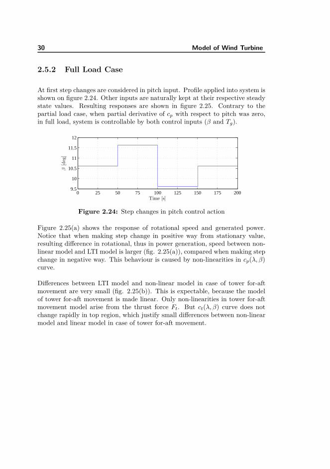
2.5.2 Full Load Case
At first step changes are considered in pitch input. Profile applied into system isshown on figure 2.24. Other inputs are naturally kept at their respective steadystate values. Resulting responses are shown in figure 2.25. Contrary to thepartial load case, when partial derivative of cp with respect to pitch was zero,in full load, system is controllable by both control inputs (β and Tg).
0 25 50 75 100 125 150 175 2009.5
10
10.5
11
11.5
12
β[deg]
Time [s]
Figure 2.24: Step changes in pitch control action
Figure 2.25(a) shows the response of rotational speed and generated power.Notice that when making step change in positive way from stationary value,resulting difference in rotational, thus in power generation, speed between non-linear model and LTI model is larger (fig. 2.25(a)), compared when making stepchange in negative way. This behaviour is caused by non-linearities in cp(λ, β)curve.
Differences between LTI model and non-linear model in case of tower for-aftmovement are very small (fig. 2.25(b)). This is expectable, because the modelof tower for-aft movement is made linear. Only non-linearities in tower for-aftmovement model arise from the thrust force Ft. But ct(λ, β) curve does notchange rapidly in top region, which justify small differences between non-linearmodel and linear model in case of tower for-aft movement.

2.5 Step Responses 31
0 25 50 75 100 125 150 175 20010.5
11.3
12.1
12.9
13.7ωr[rpm]
Non−linearLTI
0 25 50 75 100 125 150 175 2004.5
4.75
5
5.25
5.5x 10
6
Pe[W
]
Time [s]
(a) Measurements - Pe and ωr
0 25 50 75 100 125 150 175 2000.1
0.2
0.3
0.4
xt[m
]
Non−linearLTI
0 25 50 75 100 125 150 175 200−0.2
−0.1
0
0.1
0.2
xt[m
/s]
Time [s]
(b) Tower displacement xt and speed of displacement xt
Figure 2.25: Response to change in pitch (β) control input (fig. 2.24)

32 Model of Wind Turbine
Second input taken into to consideration is generator torque. Step changes,which are applied to system are shown on figure 2.26. The relation betweengenerator torque input and rotational speed is linear, so only small differencesbetween non-linear model and LTI model are expected. Direct connection be-tween generator torque input and power generator results in step response shownin figure 2.28(a). The tower for-aft movement is effected only by changes in therotational speed, and by the generator torque directly, so small changes areoccurring in tower for-aft displacement and speed of the displacement 2.28(b).
0 25 50 75 100 125 150 175 2003.6
3.8
4
4.2
4.4
4.6x 10
4
Tg[Nm]
Time [s]
Figure 2.26: Step changes in generator torque control action
0 25 50 75 100 125 150 175 200
14
15
16
v[m
/s]
Time [s]
Figure 2.27: Step changes in wind speed
Final set of figures shows the response to wind speed step change. The windspeed profile is shown in figure 2.27. Responses and displayed on figure 2.29.

2.5 Step Responses 33
0 25 50 75 100 125 150 175 20010.5
11.3
12.1
12.9
13.7ωr[rpm]
Non−linearLTI
0 25 50 75 100 125 150 175 2004
4.5
5
5.5x 10
6
Pe[W
]
Time [s]
(a) Measurements - Pe and ωr
0 25 50 75 100 125 150 175 2000.22
0.24
0.26
xt[m
]
Non−linearLTI
0 25 50 75 100 125 150 175 200−0.01
0
0.01
xt[m
/s]
Time [s]
(b) Tower displacement xt and speed of displacement xt
Figure 2.28: Response to generator torque step change (fig. 2.26)

34 Model of Wind Turbine
0 25 50 75 100 125 150 175 20010
11.1
12.1
13.2
14.3
ωr[rpm]
Non−linearLTI
0 20 40 60 80 100 120 140 160 180 2004
4.5
5
5.5
6x 10
6
Pe[W
]
Time [s]
(a) Measurements - Pe and ωr
0 20 40 60 80 100 120 140 160 180 2000
0.1
0.2
0.3
0.4
xt[m
]
Non−linearLTI
0 25 50 75 100 125 150 175 200−0.2
−0.1
0
0.1
0.2
xt[m
/s]
Time [s]
(b) Tower displacement xt and speed of displacement xt
Figure 2.29: Response to wind step changes (fig. 2.27)

2.6 Frequency Responses 35
Figure 2.30 shown the response of tower for-aft movement to step change in thewind speed from 15 to 16 m/s. On this figure is compared structural dampingof the tower together with aerodynamic damping.
0 20 40 60 80 100 1200.22
0.24
0.26
0.28
0.3
0.32
0.34
xt[m
]
aerodynamic damping structural damping
0 20 40 60 80 100 120−0.1
−0.05
0
0.05
0.1
Time [s]
xt[m
/s]
Figure 2.30: Effect of aerodynamics to the tower for-aft movement
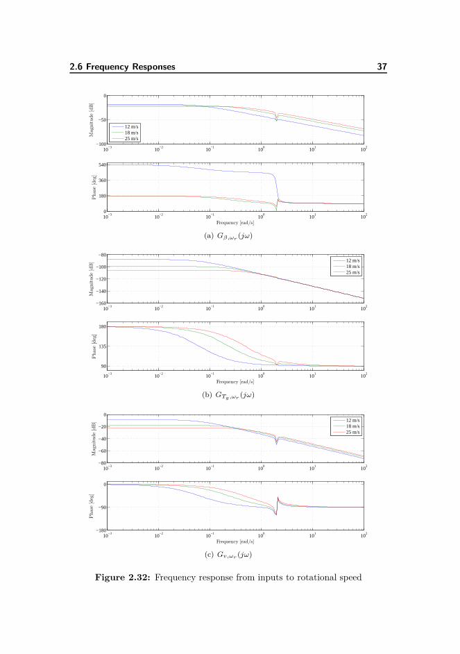
2.6 Frequency Responses
This thesis deals with design of frequency weighted MPC controller, for thatreason some frequency responses of the system are evaluated. Transfer functionfrom all inputs to all outputs and states are considered. Specifically from controlinputs β, Tg and from wind speed v to output Pe and states ωr, xt, xt. Notice,that all responses have characteristics of low-pass filter except responses of thetransfer function GTg,Pe
(jω), which has high-pass characteristic. This is causedby non-zero D matrix, in state space model.
More detailed frequency responses at all wind speeds can be found in appendixB, in which 3D bode plots are made.

36 Model of Wind Turbine
10−3
10−2
10−1
100
101
102
40
60
80
100
120
Mag
nitude[dB]
12 m/s18 m/s25 m/s
10−3
10−2
10−1
100
101
102
0
180
360
540
Phase[deg]
Frequency [rad/s]
(a) Gβ,Pe(jω)
10−3
10−2
10−1
100
101
102
30
35
40
45
Mag
nitude[dB]
12 m/s18 m/s25 m/s
10−3
10−2
10−1
100
101
102
0
90
180
Phase[deg]
Frequency [rad/s]
(b) GTg ,Pe(jω)
10−3
10−2
10−1
100
101
102
50
100
150
Mag
nitude[dB] 12 m/s
18 m/s25 m/s
10−3
10−2
10−1
100
101
102
−180
−90
0
Phase[deg]
Frequency [rad/s]
(c) Gv,Pe(jω)
Figure 2.31: Frequency response from inputs to generated power
2.6 Frequency Responses 37
10−3
10−2
10−1
100
101
102
−100
−50
0Mag
nitude[dB]
12 m/s18 m/s25 m/s
10−3
10−2
10−1
100
101
102
0
180
360
540
Phase[deg]
Frequency [rad/s]
(a) Gβ,ωr(jω)
10−3
10−2
10−1
100
101
102
−160
−140
−120
−100
−80
Mag
nitude[dB] 12 m/s
18 m/s25 m/s
10−3
10−2
10−1
100
101
102
90
135
180
Phase[deg]
Frequency [rad/s]
(b) GTg ,ωr(jω)
10−3
10−2
10−1
100
101
102
−80
−60
−40
−20
0
Mag
nitude[dB] 12 m/s
18 m/s25 m/s
10−3
10−2
10−1
100
101
102
−180
−90
0
Phase[deg]
Frequency [rad/s]
(c) Gv,ωr (jω)
Figure 2.32: Frequency response from inputs to rotational speed

38 Model of Wind Turbine
10−3
10−2
10−1
100
101
102
−100
−50
0
Mag
nitude[dB] 12 m/s
18 m/s25 m/s
10−3
10−2
10−1
100
101
102
0
180
360
Phase[deg]
Frequency [rad/s]
(a) Gβ,xt(jω)
10−3
10−2
10−1
100
101
102
−250
−200
−150
−100
Mag
nitude[dB]
12 m/s18 m/s25 m/s
10−3
10−2
10−1
100
101
102
−360
−180
0
180
Phase[deg]
Frequency [rad/s]
(b) GTg ,xt(jω)
10−3
10−2
10−1
100
101
102
−100
−50
0
Mag
nitude[dB] 12 m/s
18 m/s25 m/s
10−3
10−2
10−1
100
101
102
−180
−90
0
90
180
Phase[deg]
Frequency [rad/s]
(c) Gv,xt (jω)
Figure 2.33: Frequency response from inputs to tower for-aft displacement

2.6 Frequency Responses 39
10−3
10−2
10−1
100
101
102
−150
−100
−50
0Mag
nitude[dB]
12 m/s18 m/s25 m/s
10−3
10−2
10−1
100
101
102
90
180
270
360
450
Phase[deg]
Frequency [rad/s]
(a) Gβ,xt(jω)
10−3
10−2
10−1
100
101
102
−250
−200
−150
−100
−50
Mag
nitude[dB] 12 m/s
18 m/s25 m/s
10−3
10−2
10−1
100
101
102
−180
−90
0
90
180
270
Phase[deg]
Frequency [rad/s]
(b) GTg ,xt(jω)
10−3
10−2
10−1
100
101
102
−150
−100
−50
0
Mag
nitude[dB]
12 m/s18 m/s25 m/s
10−3
10−2
10−1
100
101
102
−90
0
90
180
270
Phase[deg]
Frequency [rad/s]
(c) Gv,xt (jω)
Figure 2.34: Frequency response from inputs to tower for-aft speed of dis-placement

40 Model of Wind Turbine

Chapter 3
Wind Speed Estimation and
Disturbance Modelling
Model Predictive Control is a state feedback control. This means, that esti-mation of the states is required. Since we are not measuring the wind speed,estimation of this quantity is required as well. Based on the estimation of thewind speed, linearisation point and system dynamics are changed. Last signalsthat needed to be estimated, are unmeasured input and output disturbances, sooffset-free regulation is achieved.
3.1 Wind Speed Estimation
In real world application, where the wind speed is varying throughout rotordisc, it is difficult to measure reliably the wind speed. Due to this fact, thewind turbine itself serves as a measurement device of the wind speed. Severalmethods has been proposed how to achieve satisfactory wind speed estimation.Very common approach is to use stationary Kalman filter, like proposed in (Xinet al., 1997). Approach proposed by (Bourlis and Bleijs, 2010), demonstratesusage of adaptive Kalman filter. Another approach presented by (Østergaardet al., 2007) is to use Kalman filter to estimate rotor speed and aerodynamictorque, and using equation 3.1 to calculate λ. Once λ is known, wind speed can

42 Wind Speed Estimation and Disturbance Modelling
be easily calculated. This concept proven to be working without any problemsonly in wind speed range from 10 to 14 m/s. At other wind speed numericaldifficulties arise during solving equation 3.1 for λ, and also the fact, that cp
curve is concave, which means that for two different λ values, same cp value iscalculated.
QrωR =12
ρπR2 R3ω3r
λ3cp(λ, β) (3.1)
In this project very well known stationary predictive Kalman filter (Poulsen,2007) has been used in order to estimate the wind speed. Satisfactory resultshave been obtain using this strategy.
3.2 Disturbance Modelling
Disturbance modelling has proven to be very effective in order to estimateunmeasured disturbances and mismatch between linear and non-linear model.Once these disturbances are estimated, MPC algorithm can be easily modified,so these disturbances are rejected (Pannocchia and Rawlings, 2003).
The main idea behind this approach, is to augment discrete time state spacemodel (eq. 3.2) with number of integrating disturbances. Specially in our casewe have to take to account the estimation of the wind speed as well. Based onthis augmented system description predictive Kalman filter is designed.
Original state space description in discrete time:
xk+1 = Axk + Buk + Bvvk + Exdk + γk (3.2)
yk = Cxk + Duk + Eydk + ηk (3.3)
where xk are the state variables at given sample k, uk is the control input vector.vk is the wind speed, dk are unmeasured disturbances, γ and η are process andmeasurement noise.
Statistical characteristics of the noise variables are:
γ ∈ Niid(0, Qe) η ∈ Niid(0, Re) (3.4)

3.2 Disturbance Modelling 43
Considered state variables in the augmented system (eq. 3.6) are, x denotesstate variables of original system state space description, xv are state variableslinked to wind speed model, and d are estimated disturbances.
xxv
d
k+1
=
A Bv Ex
0 Aw 00 0 I
xxv
d
k
+
B00
uk + γk (3.5a)
yk =[
C 0 Ey
]
xxv
d
k
+ Duk + ηk (3.5b)
yielding:
xk+1 = Aexk + Beuk + γk (3.6a)
y = Cexk + Duk + ηk (3.6b)
The estimation takes place as follows:
xxv
d
k|k
=
xxv
d
k|k−1
+ △xs + L(
ym − yk|k−1
)
(3.7)
where △xs is the difference between steady state values of the states 3.8. Valueof △xs will remain zero, when the linearisation point does not change. In thecase of steady values of wind speed model, only steady state value of the firststate variable is non-zero. The steady state value of the second state in windspeed model as well as the disturbances has steady state values equal to zero.
△xs =
xsk−1 − xs
k[
vm,k−1 − vm,k
0
]
0
(3.8)
This correction has to be made, because the system dynamics together withlinearisation point needs to be changed during control. This will ensure, thatwhen the system dynamics changes, that the estimator will give the same result.Block diagram of the observer is shown on figure 3.1.

44 Wind Speed Estimation and Disturbance Modelling
The prediction part of the estimator is described in following equation:
xxv
d
k+1|k
=
A Bv Ex
0 Aw 00 0 I
xxv
d
k|k
+
B00
uk|k (3.9a)
yk =[
C 0 Ey
]
xxv
d
k|k
+ Duk|k (3.9b)
Figure 3.1: Structure of the linear observer
Predictor gain matrix is calculated from 3.10, which preceded by solving alge-braic Riccati equation in discrete time 3.11.
L = AeΣCT (CΣCT + R)−1 (3.10)
Σ = AeΣATe + Q − AeΣCT (CΣCT + R)−1CΣAT
e (3.11)

Chapter 4
Model Predictive Control
4.1 Standard MPC
The core of MPC lies in solving quadratic objective function with linear con-straints. Such mathematical problem is called quadratic programming (QP). Ingeneral, QP program can be expressed in following form (Boyd and Vanden-berghe, 2009):
minimize12
vT Hv + gT v + r (4.1a)
s. t. Cv � d (4.1b)
Av = b (4.1c)
where H ∈ Sn, C ∈ Rm×n, A ∈ Rp×n. In this section we will focus on formu-lating the control problem as a standard MPC problem, which we will translateinto QP formulation.
Writing the cost function with the constraints is big part of the MPC implemen-tation. There are several ways how approach this problem and it also depend onthe application. In this thesis output regulation with constraints is considered,and the optimizing variable will be the control input vector.
There are however several other approaches. Widely used is formulation, where

46 Model Predictive Control
the optimization variable is control move (△u = uk − uk−1) instead of absolutevalue of control signal (uk) (Maciejowski, 2002; Camacho and Bordons, 2007;Gosk, 2011). Another formulation arise by directly looking at the basic formu-lation (equation 4.2a) and treat both state variables and control input variablesas optimization variables (Kvasnica, 2009). This formulation has one drawbackbecause we increase the number of optimizing variables, but advantage couldbe sparsity of curvature matrix (matrix H from 4.1a), which in this case isdiagonal. In previously mentioned approach, where the optimization variableis control input vector, or control move vector, the curvature matrix is dense.This may increase the time needed for calculation, due to the fact, that duringsolving QP problem this matrix must be inverted. Another formulation whichis currently being researched, is that the control input vector is eliminated fromthe cost function and only state variables are considered as optimizing variables(Mancuso and Kerrigan, 2011).
General formulation of standard MPC problem with linear constraints is shownin eq. 4.2a. State space model represents the equality constraints. Boundson control inputs together with bounds on states represent the inequality con-straints.
Φ = minN∑
k=1
xT Qx +N−1∑
k=1
uT Ru (4.2a)
s.t. xk+1 = Axk + Buk (4.2b)
x ∈ X (4.2c)
u ∈ U (4.2d)
where N is prediction horizon, Q ∈ Rnx×nx , R ∈ R
nu×nu are weighting matri-ces. Presented formulation has several drawbacks, and it is not suited for greatportion of applications. The main issue is, that using cost function written in4.2a deviations of x, u from zero is penalized. This cannot be used for offset freecontrol unless changes are made. One of many possibilities is to introduce targetvariables (Muske and Rawlings, 1993), so the cost function will be changed infollowing manner:
Φ = minN∑
k=1
(x − xs)T Q(x − xs) +N−1∑
k=1
(u − us)T R(u − us) (4.3)
Where xs, us are steady state values. In the section (4.1.1) will be introducedanother approach to handle offset free control along with QP formulation basedon control vector as an optimization variable.
As it can be understood from the presented equations, by solving QP problemwe calculate the optimal control inputs over the prediction horizon. Once these

4.1 Standard MPC 47
inputs are applied to the plant, states of the plant are moved to different values.Such application resembles open-loop implementation. However for satisfactoryresults and offset free control, closed-loop implementation is chosen. In closed-loop application the optimization is performed at each sample, with new initialcondition (x0 = xk). In most applications the length of the horizon is preserved.Such control strategy is known as receding horizon control (RHC). RHC imple-mentation has been widely researched (e.g. (Maciejowski, 2002)) and used invarious industrial implementation i.e. (Prasath et al., 2010).
Output regulation problem formulated in 4.4 together with disturbance mod-elling (previous chapter) will achieve offset free reference tracking.
Φ =12
N∑
k=0
||rk − yk||2Q +12
N−1∑
k=0
||△uk||2R (4.4)
Where rk is the reference value for the output and yk is the measurement of theoutput. This objective function will suppress the changes in the control signal△uk. It will have no bearing on the difference between absolute value of thecontrol input and zero like in formulation 4.2a.
4.1.1 Unconstrained MPC
In this section, unconstrained MPC controller will be presented. In order tosolve optimization problem expressed in 4.4, this objective function must berewritten into form presented in 4.1a. As it was mentioned in begging of thischapter, the optimization variable will be the control inputs U over the chosenprediction horizon.
For the purpose of rewriting the MPC cost function into standard QP problem,relation between the outputs yk and inputs uk must be known. Evolution basedin state space model will be used (eq. 4.5).
xk+1 = Axk + Buk + Exdk k = 0..N (4.5a)
yk = Cxk + Duk + Eydk k = 0..N (4.5b)
Contrary to the suggested set-up in e.g. (Maciejowski, 2002), D matrix mustbe considered in MPC design for wind turbines as well.

48 Model Predictive Control
QP problem which is formulated can be expressed as a weighted least squarequadratic optimization problem 4.6, in which U⋆ is the optimal solution to theproblem. In this case weighting matrix is related to outputs; Q ∈ Rny×ny
U⋆ = min12
||Y − R||2Q +12
||△U ||2R (4.6)
This cost function can be then translated into standard QP problem shown in4.7 by exploiting the evolution of the outputs over the prediction horizon basedon state space model (eq. 4.8 through 4.13). Model without disturbances d isconsidered first.
U⋆ = min12
UT HU + gT U + r (4.7)
State space evolution for sample k = 1:
xk+1 = Axk + Buk (4.8)
yk = Cxk + Duk (4.9)
State space evolution for sample k = 2:
xk+2 = Axk+1 + Buk+1
= A(Axk + Buk) + Buk+1
= A2xk + ABuk + Buk+1
(4.10)
yk+1 = Cxk+1 + Duk+1
= C(Axk + Buk) + Duk+1
= CAxk + CBuk + Duk+1
(4.11)
State space evolution for sample k = 3:
xk+3 = Axk+2 + Buk+2
= A(A2xk + ABuk + Buk+1) + Buk+1
= A3xk + A2Buk + ABuk+1 + Buk+2
(4.12)
yk+2 = Cxk+2 + Duk+2
= C(A2xk + ABuk + Buk+1) + Duk+2
= CA2xk + CABuk + CBuk+1 + Duk+2
(4.13)
4.1 Standard MPC 49
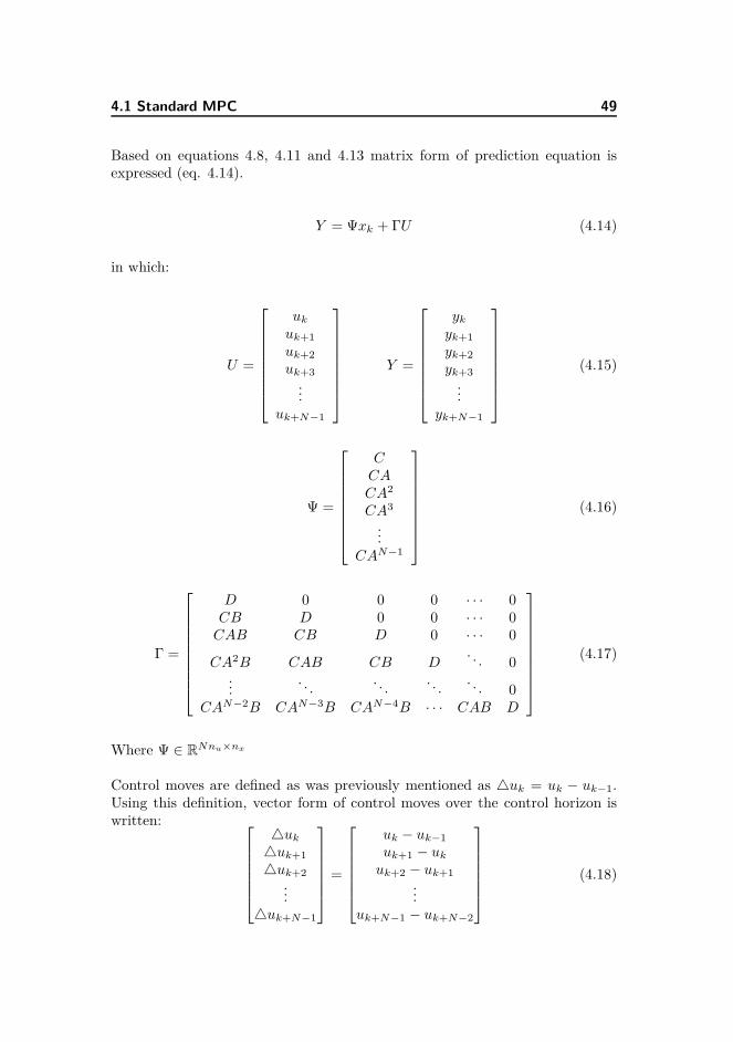
Based on equations 4.8, 4.11 and 4.13 matrix form of prediction equation isexpressed (eq. 4.14).
Y = Ψxk + ΓU (4.14)
in which:
U =
uk
uk+1
uk+2
uk+3
...uk+N−1
Y =
yk
yk+1
yk+2
yk+3
...yk+N−1
(4.15)
Ψ =
CCACA2
CA3
...CAN−1
(4.16)
Γ =
D 0 0 0 · · · 0CB D 0 0 · · · 0
CAB CB D 0 · · · 0
CA2B CAB CB D. . . 0
.... . .
. . .. . .
. . . 0CAN−2B CAN−3B CAN−4B · · · CAB D
(4.17)
Where Ψ ∈ RNnu×nx
Control moves are defined as was previously mentioned as △uk = uk − uk−1.Using this definition, vector form of control moves over the control horizon iswritten:
△uk
△uk+1
△uk+2
...△uk+N−1
=
uk − uk−1
uk+1 − uk
uk+2 − uk+1
...uk+N−1 − uk+N−2
(4.18)
50 Model Predictive Control
△uk
△uk+1
△uk+2
...△uk+N−1
=
Iu 0 0 0 0−Iu Iu 0 0 0
0 −Iu Iu 0 0
0 0. . .
. . . 00 0 0 −Iu Iu
uk
uk+1
uk+2
...uk+N−1
−
Iu
00...0
uk−1 (4.19)
where Iu ∈ Inu×nu .
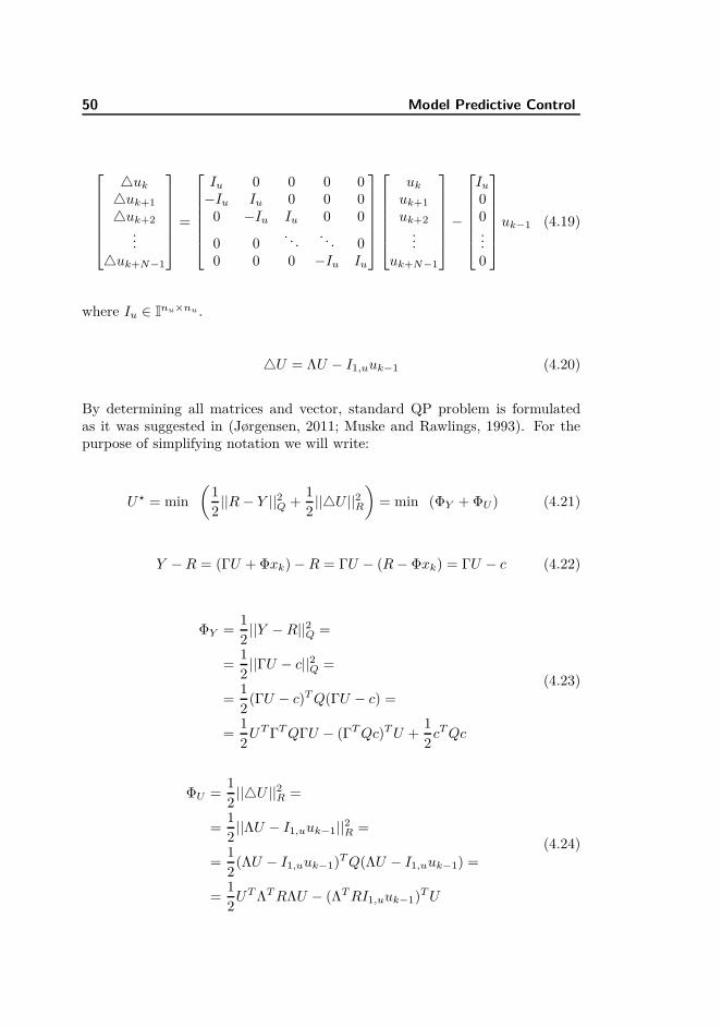
△U = ΛU − I1,uuk−1 (4.20)
By determining all matrices and vector, standard QP problem is formulatedas it was suggested in (Jørgensen, 2011; Muske and Rawlings, 1993). For thepurpose of simplifying notation we will write:
U⋆ = min(
12
||R − Y ||2Q +12
||△U ||2R
)
= min (ΦY + ΦU ) (4.21)
Y − R = (ΓU + Φxk) − R = ΓU − (R − Φxk) = ΓU − c (4.22)
ΦY =12
||Y − R||2Q =
=12
||ΓU − c||2Q =
=12
(ΓU − c)T Q(ΓU − c) =
=12
UT ΓT QΓU − (ΓT Qc)T U +12
cT Qc
(4.23)
ΦU =12
||△U ||2R =
=12
||ΛU − I1,uuk−1||2R =
=12
(ΛU − I1,uuk−1)T Q(ΛU − I1,uuk−1) =
=12
UT ΛT RΛU − (ΛT RI1,uuk−1)T U
(4.24)

4.1 Standard MPC 51
H = ΓT QΓ + ΛT RΛ (4.25)
g = −ΓT Qc − ΛT RI1,uuk−1 =
= −ΓT Q(R − Φxk) − ΛT RI1,uuk−1 =
= ΓT QR + ΓT Φxk − ΛT RI1,uuk−1
(4.26)
Equations 4.25 and 4.26 define curvature matrix H and first order coefficientvector g. In order to achieve offset free control, disturbances must be taken intoaccount. In order to this, relation between outputs y and disturbances d is found.This is done similarly to finding relation between outputs and inputs. Equation4.28 shows the matrix form of prediction equation, in which are included states,control inputs and disturbances.
ΓD =
Ey 0 0 0 · · · 0CEx Ey 0 0 · · · 0
CAEx CEx Ey 0 · · · 0
CA2Ex CAEx CEx Ey
. . . 0...
. . .. . .
. . .. . . 0
CAN−2Ex CAN−3Ex CAN−4Ex · · · CAEx Ey
(4.27)
Y = Ψxk + ΓU + ΓDD (4.28)
This equation is then inserted into equation 4.22, yielding equation 4.29. By con-tinuing derivation like it was presented in eq. 4.24 through 4.26. The curvaturematrix H will remain unchanged, but the g vector will be change accordingly(eq. 4.30).
Y − R = (Ψxk + ΓU + ΓDD) − R = ΓU − (R − Φxk − ΓDD) = ΓU − c (4.29)
g = ΓT QR + ΓT QΦxk − ΛT RI1,uuk−1 + ΓT QΓDD (4.30)

52 Model Predictive Control
For the purpose of simplifying notation, equation 4.30 is rewritten into:
g = MRR + Mxxk + Muuk−1 + MDD (4.31)
Final formulation presented in eq. 4.32 can be solved by numerous algorithmse.g. active-set algorithms (Nocedal and Wright, 1999). The tools solving QPproblems used in this project were namely quadprog() in Matlab and fasterversion of QP solver qpas() (Wills, 2007).
Ustar = min12
UT HU + gT U (4.32)
4.1.2 Hard Constraints
The main advantage of MPC is to handle constraints. Incorporating constraintsinto main QP problem is done as it is suggested in 4.1a. These constraintshave form of linear inequality equations 4.33. In this section we will presentthe formulation of hard constraints on control inputs u, control moves △u andoutputs y. Since we are dealing with stable system, constraints on systemstates may not be considered. However, if MPC is used on unstable process,then constraints on states should be considered.
umin ≤ uk ≤ umax k = 0..N − 1△umin ≤ △uk ≤ △umax k = 0..N − 1ymin ≤ yk ≤ ymax k = 0..N
(4.33)
Constraints presented in 4.33 must be rewritten into matrix form. The boundson control signal are just stacked like in 4.34. Using definition of Λ matrix fromeq. 4.20, matrix form of inequality constraints for control moves are expressedin eq. 4.35 yielding 4.36.
Umin =
umin
umin
...umin
Umax =
umax
umax
...umax
(4.34)

4.1 Standard MPC 53
△umin + uk−1
△umin
...△umin
≤ ΛU ≤
△umax + uk−1
△umax
...△umax
(4.35)
△Umin + I1,uuk−1 ≤ ΛU ≤ △Umax + I1,uuk−1 (4.36)
Next formulation of output constraints is going to take place (eq. 4.37 and 4.38).Relation between matrix form of output and control inputs is used (eq. 4.28).Bounds on outputs Ymin and Ymax are created similarly as bound on inputs (eq.4.34).
Ymin ≤ Ψxk + ΓU + ΓDD ≤ Ymax (4.37)
Ymin − (Ψxk + ΓDD) ≤ ΓU ≤ Ymax − (Ψxk + ΓDD) (4.38)
Constraints defined in equations 4.36 and 4.38 can be put together resulting in4.39.
[
△Umin + I1,uuk−1
Ymin − (Ψxk + ΓDD)
]
≤
[
ΛΓ
]
U ≤
[
△Umax + I1,uuk−1
Ymax − (Ψxk + ΓDD)
]
(4.39)
Most of the already mentioned solvers require formulation like presented in 4.1a,so 4.39 must be reformulated as shown in 4.40.
ΛΓ
−Λ−Γ
U ≤
△Umax + I1,uuk−1
Ymax − (Ψxk + ΓDD)−△Umin + I1,uuk−1
−(Ymin − (Ψxk + ΓDD))
(4.40)
4.1.3 Soft Constraints
In general, hard constraints on output should be avoided due to the infeasi-bility issues, which may arise. It is strongly recommended to implement soft

54 Model Predictive Control
constraints at least on the outputs, so the QP problem has always a solution(Prasath and Jørgensen, 2009; Zeilinger et al., 2010). Having hard constraintson control inputs, or control moves do not create the risk of running into infeasi-bility. These infeasibility issues arise mainly if we consider stochastic influenceson the process, measurements can easily cross the hard limit we set in the con-straints (Primbs, 2007). It is also a good practise to introduce soft constraints oninputs as well, so if it is necessary to ensure reference tracking, or in case of windturbine disturbance rejection, MPC controller can achieve better performance.
Implementing soft constraints into QP problem has, however significant draw-back. The soft margins (slack variables), we are introducing on outputs or inputsare becoming optimization variables as well. Objective function which needs tobe minimized is shown in 4.41. It is clear, that increased complexity of theQP problem, may prolong the calculation time. In the new objective function,matrices Su and Sy are weighting matrices related to the slack variables.
Φ =12
N∑
k=0
||rk − yk||2Q +12
N∑
k=0
||wy,k||2Sy+
12
N−1∑
k=0
||△uk||2R +12
N−1∑
k=0
||wu,k||2Su
(4.41)
First, soft constraints on inputs is being considered 4.42. By introducing theslack variable wu,k we allow crossing the limit △umin and △umax. As it wasalready mentioned, this slack variable will become optimization variable like U ,so different and very high penalty is going to be applied for the soft margin, sothe MPC controller will be "reluctant" to cross the limit.
△umin − wu,k ≤ △uk ≤ △umax + wu,k (4.42)
△Umin − Wu ≤ △U ≤ △Umax + Wu (4.43)
Soft input constraints (eq. 4.43) must be rewritten into matrix form, which issuitable for most of the QP solvers 4.44. This has been already presented in eq.4.40.
[
Λ −Iu,N
−Λ −Iu,N
] [
UWu
]
≤
[
△Umax
−△Umin
]
(4.44)
4.1 Standard MPC 55
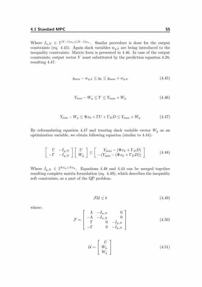
Where Iu,N ∈ I(N−1)nu×(N−1)nu . Similar procedure is done for the outputconstraints (eq. 4.45). Again slack variables wy,k are being introduced to theinequality constraints. Matrix form is presented in 4.46. In case of the outputconstraints, output vector Y must substituted by the prediction equation 4.28,resulting 4.47.
ymin − wy,k ≤ yk ≤ ymax + wy,k (4.45)
Ymin − Wy ≤ Y ≤ Ymax + Wy (4.46)
Ymin − Wy ≤ Ψx0 + ΓU + ΓDD ≤ Ymax + Wy (4.47)
By reformulating equation 4.47 and treating slack variable vector Wy as anoptimization variable, we obtain following equation (similar to 4.44):
[
Γ −Iy,N
−Γ −Iy,N
] [
UWy
]
≤
[
Ymax − (Ψxk + ΓDD)−(Ymin − (Ψxk + ΓDD))
]
(4.48)
Where Iy,N ∈ INny×Nny . Equations 4.48 and 4.44 can be merged togetherresulting complete matrix formulation (eq. 4.49), which describes the inequalitysoft constraints, as a part of the QP problem.
FU ≤ b (4.49)
where:
F =
Λ −Iu,N 0−Λ −Iu,N 0
Γ 0 −Iy,N
−Γ 0 −Iy,N
(4.50)
U =
UWu
Wy
(4.51)
56 Model Predictive Control
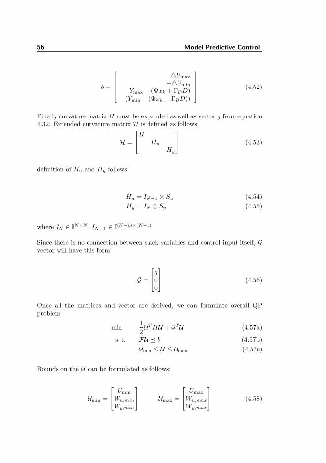
b =
△Umax
−△Umin
Ymax − (Ψxk + ΓDD)−(Ymin − (Ψxk + ΓDD))
(4.52)
Finally curvature matrix H must be expanded as well as vector g from equation4.32. Extended curvature matrix H is defined as follows:
H =
HHu
Hy
(4.53)
definition of Hu and Hy follows:
Hu = IN−1 ⊗ Su (4.54)
Hy = IN ⊗ Sy (4.55)
where IN ∈ IN×N , IN−1 ∈ I(N−1)×(N−1)
Since there is no connection between slack variables and control input itself, Gvector will have this form:
G =
g00
(4.56)
Once all the matrices and vector are derived, we can formulate overall QPproblem:
min12
UT HU + GT U (4.57a)
s. t. FU � b (4.57b)
Umin ≤ U ≤ Umax (4.57c)
Bounds on the U can be formulated as follows:
Umin =
Umin
Wu,min
Wy,min
Umax =
Umax
Wu,max
Wy,max
(4.58)

4.2 Frequency Weighted MPC 57
Where Wu,y,min is set to zero, and Wu,y,max is usually set to certain number,which is called soft margin. Slightly different approach to soft constraints isproposed by (Prasath and Jørgensen, 2009), where vector Wu,y,max is set toinfinity. This however means, that at certain circumstances (i.e. bad tuning)the controller can use control action of arbitrary magnitude.
4.2 Frequency Weighted MPC
Frequency weighted MPC (FMPC) control combines the advantages of modelpredictive control together with frequency weighting trough introducing filtersinto control loop (Poulsen, 2007). By introducing these filters into control sys-tem, tuning of the controller is shifted from standard weighting matrices (e.g.Q and R from previous section) to specifying the filters. Introducing filters intocontrol system allows us to penalize certain frequency content on each signalseparately. In case of wind turbine control, is desirable for example to penalizecertain frequencies of the tower for-aft movement. However different frequencycontent is penalized in case of control inputs. As it was indicated, these filtersare being put on control inputs, states and outputs as well, like shown in eq.4.59.
xf1...
xfn
=
Gx,1(s). . .
Gx,n(s)
x1
...xn
(4.59a)
yf1...
yfm
=
Gy,1(s). . .
Gx,m(s)
y1
...ym
(4.59b)
uf1...
ufi
=
Gu,1(s). . .
Gu,i(s)
u1
...ui
(4.59c)
This transfer function matrices can be very easily represented in state spaceform.
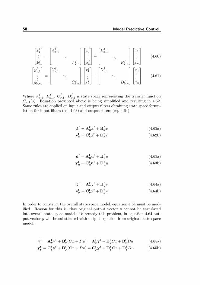
58 Model Predictive Control
xf1...
xfn
=
Afx,1
. . .Af
x,n
xf1...
xfn
+
Bfx,1
. . .Bf
x,n
x1
...xn
(4.60)
yfx,1...
yfx,n
=
Cfx,1
. . .Cf
x,n
xf1...
xfn
+
Dfx,1
. . .Df
x,n
x1
...xn
(4.61)
Where Afx,1, Bf
x,1, Cfx,1, Df
x,1 is state space representing the transfer functionGx,1(s). Equation presented above is being simplified and resulting in 4.62.Same rules are applied on input and output filters obtaining state space formu-lation for input filters (eq. 4.63) and output filters (eq. 4.64).
xf = Afxxf + Bf
xx (4.62a)
yfx = Cf
xxf + Dfxx (4.62b)
uf = Afuuf + Bf
uu (4.63a)
yfu = Cf
uuf + Dfuu (4.63b)
yf = Afyyf + Bf
yy (4.64a)
yfy = Cf
yyf + Dfyy (4.64b)
In order to construct the overall state space model, equation 4.64 must be mod-ified. Reason for this is, that original output vector y cannot be translatedinto overall state space model. To remedy this problem, in equation 4.64 out-put vector y will be substituted with output equation from original state spacemodel.
yf = Afyyf + Bf
y(Cx + Du) = Afyyf + Bf
yCx + BfyDu (4.65a)
yfy = Cf
yyf + Dfy(Cx + Du) = Cf
yyf + DfyCx + Df
yDu (4.65b)
4.2 Frequency Weighted MPC 59
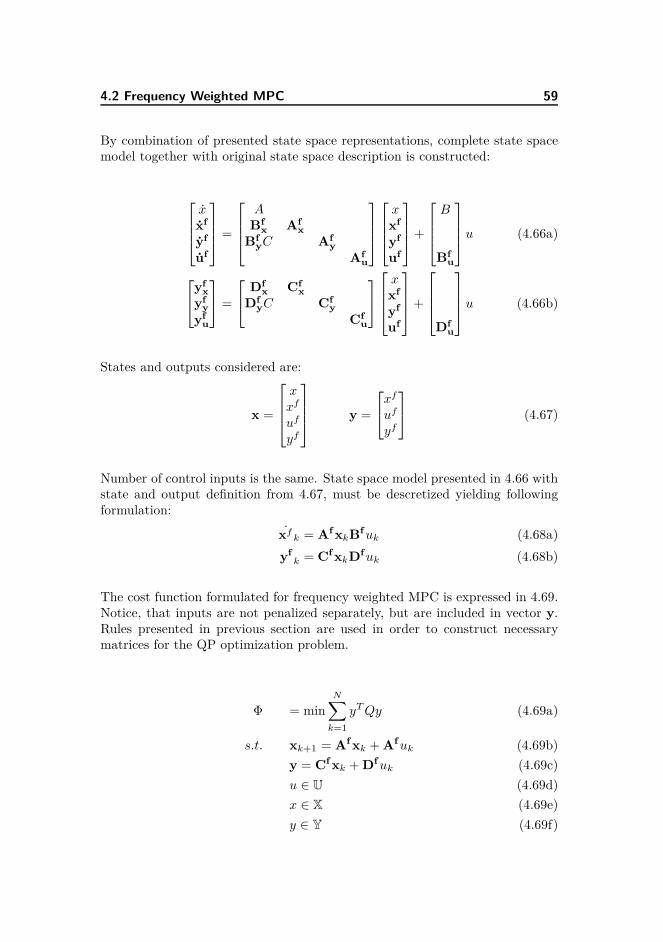
By combination of presented state space representations, complete state spacemodel together with original state space description is constructed:
xxf
yf
uf
=
ABf
x Afx
BfyC Af
y
Afu
xxf
yf
uf
+
B
Bfu
u (4.66a)
yfx
yfy
yfu
=
Dfx Cf
x
DfyC Cf
y
Cfu
xxf
yf
uf
+
Dfu
u (4.66b)
States and outputs considered are:
x =
xxf
uf
yf
y =
xf
uf
yf
(4.67)
Number of control inputs is the same. State space model presented in 4.66 withstate and output definition from 4.67, must be descretized yielding followingformulation:
xfk = Af xkBf uk (4.68a)
yfk = Cf xkDf uk (4.68b)
The cost function formulated for frequency weighted MPC is expressed in 4.69.Notice, that inputs are not penalized separately, but are included in vector y.Rules presented in previous section are used in order to construct necessarymatrices for the QP optimization problem.
Φ = minN∑
k=1
yT Qy (4.69a)
s.t. xk+1 = Af xk + Af uk (4.69b)
y = Cf xk + Df uk (4.69c)
u ∈ U (4.69d)
x ∈ X (4.69e)
y ∈ Y (4.69f)

60 Model Predictive Control
General rule for the frequency tuning says, that high-pass filter should be con-sidered on inputs, and low pass filters on states and outputs (Skogestad andPostlethwaite, 2005). The main reason for using high-pass filters on inputs ispenalizing high frequency activity of the controller. Implementing low-pass filteron inputs its may move eigenvalues of the closed loop system closer to stabil-ity margin. In case of wind turbine and tower for-aft movement, high-pass orrather band-pass filters are implemented, because tower oscillations should bedampened. This tuning will be explained in detail in chapter 5.
Chapter 5
Model Predictive Control
Design for HAWT
5.1 Main Design
In this chapter, tuning of the MPC strategies and the estimator will be discussed.Control objective in partial load is to maximize the power. Due to the fact, thatthe linear model is not controllable by pitch action in partial load, only generatortorque is considered as control input. Pitch action in partial load is calculatedin order to maximize cp value for given TSR. TSR is given by the estimate ofthe wind speed and measurement of the rotational speed. Based on this fact,two consequences arise:
1. Oscillations in tower for-aft movement can not by damped actively, be-cause the link between generator torque action and tower for-aft movementis extremely week (step responses section 2.5)
2. Introducing filters and using FMPC is not relevant in partial load. Sincethe primary objective is to maximize the power, all available control ac-tivity of generator torque must be put into fulfilling this task

62 Model Predictive Control Design for HAWT
In top region, both control inputs are considered. Primary objective of thecontroller would be to keep rotational speed and power output at its respectivenominal values. In this case introducing filters and using FMPC proves to bea relevant step, because it allows us to minimize the stress effecting the planteven further than the standard MPC.
In case of standard MPC approach, state space matrices already presented inmodelling section are used in order to design the MPC Controller. Rules men-tioned in section 4.1 are applied, and QP is formulated. However, in case ofFMPC, state space model must be first introduced. After deriving the statespace model for original model and filters, QP problem can be formulated.
5.1.1 Model Scaling
In order to avoid numerical problems during solving quadratic programming,state space model has been scaled. Scaling took place on the inputs as well ason the outputs. Since there are huge differences in magnitude of inputs signals:
β0 ∈< −1.56; 23.35 > deg Tg ∈< 0.73; 40.68 > kNm (5.1)
scaling factor for pitch input has been chosen as fβ = 22 deg. Scaling factor forgenerator torque action has been chosen as fTg
= 45 kNm. Stationary valuesof inputs signals will belong to the intervals expressed in 5.2. After applyingsuch scaling to the state space model, values of B matrix will be levelled-up (eq.5.3).
β0 ∈< −0.07; 1.06 > Tg ∈< 0.02; 0.90 > (5.2)
B =
−0.0158 −2.5021 · 10−6
0 0−0.1490 0
B =
−0.3484 −0.11260 0
−3.2781 0
(5.3)
Similar scaling is done for the power output, where the unscaled C and D

5.1 Main Design 63
matrices have this shape:
C =
3945990 0 01 0 00 0 1
D =
0 122.90960 00 0
(5.4)
After applying scaling factor fTgon generator torque action, values in C matrix
will still have different order of magnitude. First row of output equation isdivided by gear coefficient Ng = 97 yielding:
C =
0.9040 0 01 0 00 0 1
D =
0 1.26710 00 0
(5.5)
Note, that these scaling factors can be chosen differently. These scaling factorsprove to result in better levelled curvature matrix H . These examples of matriceshave been given for wind speed equal to 15 m/s. The entire state space model,in C-Time is presented in A.
5.1.2 Standard MPC
Table 5.1 shows the tuning parameters of MPC controller in all four regions,and table 5.2. Satisfactory results in simulations were obtained using only oneset of weighting matrices in each region. The order of state variables, controlinputs and system outputs is:
x =
ωr
xt
xt
u =[
βTg
]
y =
Pe
ωr
xt
(5.6)
except partial load, when only generator torque is considered as control input.
Order of the states in disturbance model is:
x =[
ωr xt xt v v d]T
(5.7)

64 Model Predictive Control Design for HAWT
Table 5.1: Tuning parameters for standard MPC controller
Region 1 Region 2 Region 3 Region 4R 1e-2 1e-3 1e0 [1e1 1e-1]Q [1e-1, 1e1, 1e-1] [1e-1, 1e1, 1e0] [1e0, 1e0, 1e0]Su 1e3 [1e3, 1e3]Sy [1e5, 1e5, 1e5]
In table 5.2, there are three sets of matrices. Input covariance matrix Qe is splitinto two separate matrices Qe,x and Qe,d. While the matrix Qe,x indicate settingof covariance matrix for state estimation, covariance matrix Qe,d shows thetuning for wind speed estimation, and additional disturbances. These matricesshould be then place together as it is stated in eq. 5.21.
Qe =[
Qe,x
Qe,d
]
(5.8)
Table 5.2: Tuning parameters for stationary predictive Kalman filter
Region 1 Region 2Qe,x [1e-3, 1e0, 1e0] [1e-3, 1e1, 1e0]Qe,d [1e1, 1e1, 1e1] [1e1, 1e1, 1e-5]Re [1e-3, 1e-3, 1e-3] [1e-1, 1e-3, 1e-3]
Region 3 Region 4Qe,x [1e-3, 1e0, 1e0] [1e-3, 1e1, 1e0]Qe,d [1e2, 1e2, 1e-2] [1e1, 1e1, 1e0, 1e0]Re [1e-3, 1e-3, 1e-3] [1e-3, 1e-3, 1e-3]
In partial load only one output disturbance is considered, and namely only onrotational speed. In full load, two output disturbances are considered, specifi-cally output disturbances on generated power and on rotational speed.
In partial load, disturbances matrices has this form:
Ex =
000
Ey =
010
(5.9)
Putting disturbances on input should be avoided. Since predictive Kalman filteris used also on wind speed estimation, which is considered as input disturbance,

5.1 Main Design 65
putting additional disturbances will worsen the wind speed estimation. Since theprimary objective is to maximize the power, through controlling the rotationalspeed, putting only one output disturbance proven to be enough.
If one would be considering disturbances on the input, values in Ex matrixplays huge role. Numbers in Ex matrix must not be greater than the maximumnumber for given row in Bv matrix. In opposite case, wind speed estimationwill degrade, even when low coefficient in Qe,d matrix is placed.
Same goes for estimation in full load. Considered disturbances on power gener-ation and rotational speed (eq. 5.10) proven to yield satisfactory results.
Ex =
0 00 00 0
Ey =
1 00 10 0
(5.10)
Gain of the predictive Kalman filter L is then calculated using dlqe commandin Matlab .
It must be also noted, that these simulations were performed on model mentionin modelling section (section 2.1). If such controller will be implemented on morecomplex model e.g. FAST (Jonkman and Buhl Jr., 2005), different settings ofdisturbances should be considered.
Prediction horizons considered in standard MPC are:
N = 3s = 30 samples
5.1.3 Frequency Weighted MPC
In this subsection tuning parameters for frequency weighted MPC will be dis-cussed. First, order of considered states variables is presented:
x =[
ωr xt xt ωfr xf
t xft P f
e uf1 uf
2
]T(5.11)
Order of outputs variables considered in FMPC design:
yf =[
ωfr xf
t xft P f
e uf1 uf
2
]T(5.12)

66 Model Predictive Control Design for HAWT
As mentioned in previous chapter in FMPC tuning, is shifted from weightingmatrices Q and R, into transfer function design. However, tuning matrix Q ispresent in this design as well, but it is set to identity matrix, except coefficientsrelated to control inputs, which has been lowered (eq. 5.13). In such case,controller has more "freedom" to move from steady state point.
Q = diag([1, 1, 1, 1, 10−2, 10−2]) (5.13)
Filters placed on the control inputs have high-pass characteristic:
Hβ(s) =40s + 110s + 1
(5.14a)
HTg(s) =
100s + 14s + 1
(5.14b)
Filter placed on the the rotational speed is characterised as low-pass filter andon the states related to tower movement, has type of band-pass filter:
Hωr=
0.25s + 10.5s + 1
(5.15a)
Hxt=
s2 + 3s + 1s2 + s + 1
(5.15b)
Hxt=
s2 + 6s + 1s2 + s + 1
(5.15c)
Filter placed on power output has also low-pass characteristics:
HPe(s) =
0.1s + 12s + 1
(5.16)
Due to the fact, that rotational speed and speed of the tower are directly mea-sured states, filters on these outputs are not placed. Frequency responses ofpresented filters are shown on figures 5.1, 5.2 and 5.3.
For FMPC linear observer in form of stationary predictive Kalman filter hasbeen designed as well. Considered order of state variables is:
x =[
x v v d]T
(5.17)

5.1 Main Design 67
10−4
10−3
10−2
10−1
100
101
102
103
104
0
10
20
30Magnitude[dB] Hβ
HTg
10−4
10−3
10−2
10−1
100
101
102
103
104
0
45
90
Phase[deg]
Frequency [rad/s]
Figure 5.1: Frequency responses of the input filters
10−4
10−3
10−2
10−1
100
101
102
103
104
0
5
10
15
20
Magnitude[dB] Hxt
Hxt
10−4
10−3
10−2
10−1
100
101
102
103
104
−45
0
45
Phase[deg]
Frequency [rad/s]
Figure 5.2: Frequency responses of filters related to tower for-aft movement
10−4
10−3
10−2
10−1
100
101
102
103
104
−30
−20
−10
0
Magnitude[dB]
Hωr
HPe
10−4
10−3
10−2
10−1
100
101
102
103
104
−90
−45
0
Phase[deg]
Frequency [rad/s]
Figure 5.3: Frequency responses of the output filter and filter on rotationalspeed

68 Model Predictive Control Design for HAWT
Outputs considered in predictive Kalman filter:
y =[
Pe ωr xt yf]T
(5.18)
Two disturbances are considered similarly to standard MPC design. They areplaced on outputs, on filtered measurement of generated power and on the fil-tered measurement of rotational speed. Output disturbance matrix has followingstructure:
Ey =
0 10 00 01 00 00 0
(5.19)
Input disturbance matrix Ex is set to zero matrix with appropriate size.
Tuning of the Kalman filter state covariance matrix is:
Qe,x = diag([10−3, 10, 1]) (5.20a)
Qe,xf = diag([10−3, 10−3, 10−3, 10−3, 10−3, 10−3]) (5.20b)
Qe,d = diag([10, 10, 1, 1]) (5.20c)
Where Qx is diagonal matrix related to original states, Qxf is diagonal matrixrelated to filtered states and Qd is diagonal matrix related to wind speed modeland additional disturbances. Notice, that Qx and Qd is the same, like in caseof Kalman filter for standard MPC in top region. State covariance matrix Qe,upon which is Kalman filter design based is:
Qe =
Qe,x
Qe,xf
Qe,d
(5.21)
Output covariance matrix is constructed in same way, but following tuning:

5.2 Operational Constraints 69
Re,y = diag([10−3, 10−3, 10−3]) (5.22a)
Re,yf = diag([10−1, 10−1, 10−1, 10−1, 10−1, 10−1]) (5.22b)
(5.22c)
It may seem, that too much state variables are estimated, or too much measure-ments is used, but Matlab implementation was straight forward in this way.Also we should keep in mind, when this controller is going to be used on morecomplex models, disturbance placement may need to be revisited.
Prediction horizons considered in frequency weighted MPC are:
N = 3s = 30 samples
These horizons prove to be the minimum prediction horizon, when satisfactoryperformance of the controller has been achieved. Prolonging the horizon did notyield significantly better performance, but it has decreased the computationaltime. It must be noted, when actuators are implemented, setting for predictionhorizon should be revisited.
5.2 Operational Constraints
Operational constraints implemented in MPC controllers are stated in table 5.3.Scaled and sampled values are presented as well. Sampling frequency of 10 Hzis used in simulations.
Table 5.3: Operational Constraints
Nominal Scaled Scaled Sampledβmax 30 [deg] 1.3636 [deg] 1.3636 [deg]βmin -5 [deg] -0.2273 [deg] -0.2273 [deg]△βmax 8 [deg/s] 0.3636 [deg/s] 0.0364 [deg per sample]△βmin -8 [deg/s] -0.3636 [deg/s] -0.0364 [deg per sample]Tg,max 47403 [Nm] 1.0534 [Nm] 1.0534 [Nm]Tg,min 0 [Nm] 0 [Nm] 0 [Nm]△Tg,max 15000 [Nm/s] 0.3333 [Nm/s] 0.0333 [Nm per sample]△Tg,min -15000 [Nm/s] -0.3333 [Nm/s] -0.0333 [Nm per sample]

70 Model Predictive Control Design for HAWT
Constraints on rotational speed was originally put as 5 to 10% above or belowmaximum and minimum values, but it proves to be not necessary, because theseconstraints were never active. Same goes for generated power. However, thiscould be only case, that fairly simple model of turbine has been used on whichsimulations were performed.
Soft margin on pitch rate was set to additional 2 deg/s, soft margin for generatortorque rate was set to 5000 Nm/s.
5.3 Simulations
All simulations were performed in such way, that first wind speed profile wasgenerated. Then system dynamics matrices, optimization matrices and Kalmangains were calculated for every 0.1 m/s in the wind speed interval from 3 to25 m/s. This setting is sufficient due to the slow changes in dynamics of thesystem in the partial load. On the other hand in the full load, dynamics ofthe system change rather rapidly with increasing wind speed, calculation of thematrices at specific wind speed has been taken into consideration. Specificallythe element in B matrix linking pitch angle and rotational speed is changingrapidly. To improve the performance matrices were calculated at every windspeed over 11.2 m/s. This however has significant drawback, because it increasesthe calculation time of the simulation by approximately 40%. To remedy thisproblem, interpolation procedure has been implemented, but still there wasincrease in calculation time by approximately by 20%.
Block diagram of the simulations are shown in figure 5.4(a). Figure 5.4(b) showsblock diagram of frequency weighted MPC controller. Keep in mind, that sameprocedure with changing dynamics is also applied in case of FMPC simulations.

5.3 Simulations 71
(a) Standard MPC
(b) Frequency weighted MPC
Figure 5.4: Block diagrams

72 Model Predictive Control Design for HAWT

Chapter 6
Full Load Simulations
The first set of simulation shows the performance of the controllers in the topregion. Partial load simulations will follow in the next chapter, where will be alsoshown an overall simulation, throughout entire wind speed operation interval.
Objective of the controller in the full load is to maintain the power outputand rotational speed at theirs respective nominal values (Pnom = 5 MW andωr,nom = 12.1 rpm). Secondary objective of the controller is to minimize thephysical stress on the device itself.
In full load case two MPC controllers have been tested; standard MPC andfrequency weighted MPC controllers. Both deterministic and stochastic sim-ulations are performed. Performance of the standard MPC controller will becompared with FMPC. When applied deterministic wind speed profiles, effectsof different tunings of the filters will be explored. Simulations with stochasticwind speed profile will be shown as well. Mean values and standard deviationof the signals will be compared as well.

74 Full Load Simulations
6.1 Standard MPC
Tuning of MPC controllers was presented in chapter 5. First shown simulationis for deterministic wind speed profile. Wind speed profile is shown n figure 6.1.Estimation od the wind speed is shown as well. Notice slight estimation errorwhen step change is made from 17 to 15 m/s. This can be easily neglected,because the system dynamics does not change significantly when wind speedchanges by 0.05 m/s. Also implemented disturbance modelling takes care ofslight mismatch in estimation.
0 15 30 45 60 75 90 105 12014.5
15
15.5
16
16.5
17
17.5
windspeed[m
/s]
actualestim
0 15 30 45 60 75 90 105 120−1.5
−1
−0.5
0
0.5
1
estim.error[m
/s]
Time [s]
Figure 6.1: Deterministic wind speed profile
Contrary to the partial load simulations, less only 3 step changes were appliedto the system, so the transients especially in states related to tower movementcan be seen better. This deterministic wind speed profile is used throughoutthis entire chapter, same goes for later presented stochastic wind speed profile.Measurements of power and rotational speed are shown on figure 6.2. Statesrelated to tower for-aft movement are displayed on figure 6.3. Control actionsare shown on figures 6.4 and 6.5. Constraints are active only on pitch rate.This deterministic simulation will serve as a basis for comparison with frequencyweighted MPC (section 6.2). Deterministic simulation is followed by stochasticsimulation.

6.1 Standard MPC 75
0 15 30 45 60 75 90 105 1204.9
5
5.1Pe[M
W]
Referencemeas
0 15 30 45 60 75 90 105 12011.8
12.1
12.4
ωr[rpm]
Time [s]
Figure 6.2: Measurements - Pe and ωr
0 15 30 45 60 75 90 105 1200.15
0.25
0.35
xt[m
]
0 15 30 45 60 75 90 105 120−0.2
0
0.2
xt[m
/s]
Time [s]
Figure 6.3: Tower for-aft movement
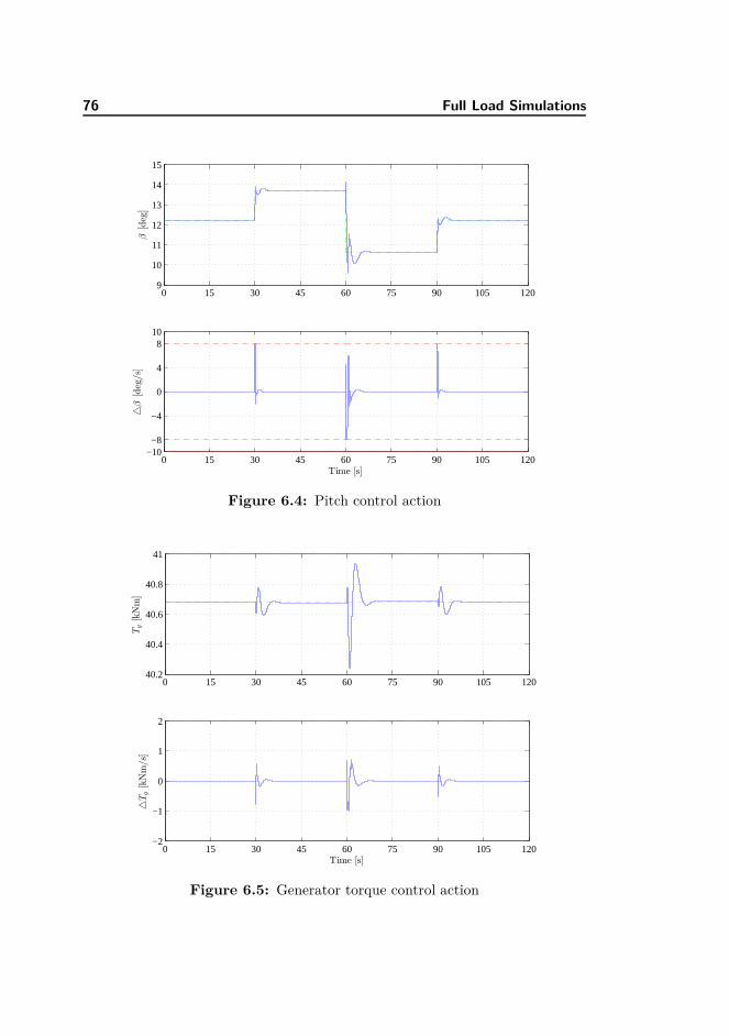
76 Full Load Simulations
0 15 30 45 60 75 90 105 1209
10
11
12
13
14
15
β[deg]
0 15 30 45 60 75 90 105 120−10−8
−4
0
4
810
△β
[deg/s]
Time [s]
Figure 6.4: Pitch control action
0 15 30 45 60 75 90 105 12040.2
40.4
40.6
40.8
41
Tg[kNm]
0 15 30 45 60 75 90 105 120−2
−1
0
1
2
△Tg[kNm/s]
Time [s]
Figure 6.5: Generator torque control action
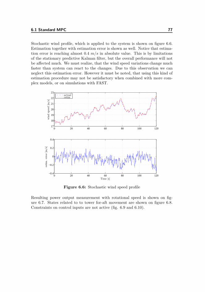
6.1 Standard MPC 77
Stochastic wind profile, which is applied to the system is shown on figure 6.6.Estimation together with estimation error is shown as well. Notice that estima-tion error is reaching almost 0.4 m/s in absolute value. This is by limitationsof the stationary predictive Kalman filter, but the overall performance will notbe affected much. We must realize, that the wind speed variations change muchfaster than system can react to the changes. Due to this observation we canneglect this estimation error. However it must be noted, that using this kind ofestimation procedure may not be satisfactory when combined with more com-plex models, or on simulations with FAST.
0 20 40 60 80 100 12017
18
19
20
21
22
23
windspeed[m
/s]
actualestim
0 20 40 60 80 100 120−0.4
−0.2
0
0.2
0.4
estim.error[m
/s]
Time [s]
Figure 6.6: Stochastic wind speed profile
Resulting power output measurement with rotational speed is shown on fig-ure 6.7. States related to to tower for-aft movement are shown on figure 6.8.Constraints on control inputs are not active (fig. 6.9 and 6.10).
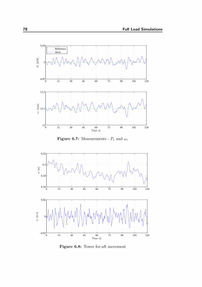
78 Full Load Simulations
0 15 30 45 60 75 90 105 1204.95
5
5.05
Pe[M
W]
Referencemeas
0 15 30 45 60 75 90 105 12012
12.1
12.2
ωr[rpm]
Time [s]
Figure 6.7: Measurements - Pe and ωr
0 15 30 45 60 75 90 105 1200.16
0.18
0.2
0.22
xt[m
]
0 15 30 45 60 75 90 105 120−0.02
0
0.02
xt[m
/s]
Time [s]
Figure 6.8: Tower for-aft movement
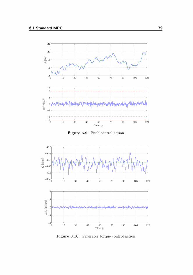
6.1 Standard MPC 79
0 15 30 45 60 75 90 105 12014
16
18
20
22β
[deg]
0 15 30 45 60 75 90 105 120−10−8
−4
0
4
810
△β
[deg/s]
Time [s]
Figure 6.9: Pitch control action
0 15 30 45 60 75 90 105 12040.55
40.6
40.65
40.7
40.75
40.8
Tg[kNm]
0 15 30 45 60 75 90 105 120−2
−1
0
1
2
△Tg[kNm/s]
Time [s]
Figure 6.10: Generator torque control action
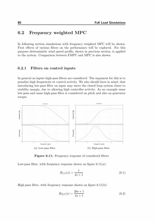
80 Full Load Simulations
6.2 Frequency weighted MPC
In following section simulations with frequency weighted MPC will be shown.First effects of various filters on the performance will be explored. For thispurpose deterministic wind speed profile, shown in previous section, is appliedto the system. Comparison between FMPC and MPC is also shown.
6.2.1 Filters on control inputs
In general on inputs high-pass filters are considered. The argument for this is topenalize high frequencies at control activity. We also should have in mind, thatintroducing low-pass filter on input may move the closed loop system closer tostability margin, due to allowing high controller activity. As an example samelow-pass and same high-pass filter is considered on pitch and also on generatortorque.
−40
−35
−30
−25
−20
−15
−10
−5
0
Mag
nitu
de (
dB)
10−2
10−1
100
101
102
−90
−45
0
Pha
se (
deg)
Bode Diagram
Frequency (rad/s)
(a) Low-pass filter
0
5
10
15
Mag
nitu
de (
dB)
10−3
10−2
10−1
100
101
0
10
20
30
40
Pha
se (
deg)
Bode Diagram
Frequency (rad/s)
(b) High-pass filter
Figure 6.11: Frequency response of considered filters
Low-pass filter, with frequency response shown on figure 6.11(a):
HLP (s) =1
4s + 1(6.1)
High-pass filter, with frequency response shown on figure 6.11(b):
HHP (s) =20s + 14s + 1
(6.2)

6.2 Frequency weighted MPC 81
Next set of figures shows the comparison of FMPC with low-pass and high-passfilters and with standard MPC controller. It must be noted, that filters only oninputs are considered so the tower oscillations are not damped. On figure 6.12are shown measurements. Tower related states are shown in figure 6.13. Cyancolor is used to show performance of the FMPC with low-pass filter on controlinputs. Simulation of FMPC with high-pass filter is shown using magenta lines.Figures 6.14 and 6.15 shows the control inputs. By blue lines is shown theperformance of the standard MPC controller. The differences of low-pass andhigh-pass filters are obvious. It must be noted, that no filter is considered fortower for-aft movement. Naturally this will poorly reflect on the overall result.But purpose of these simulations is to show the effects of different filters oninputs signals.
0 15 30 45 60 75 90 105 1204.9
5
5.1
Pe[M
W]
ReferenceMPCFMPC−LPFMPC−HP
0 15 30 45 60 75 90 105 12011.8
12.1
12.4
ωr[rpm]
Time [s]
(a) Measurements - Pe and ωr
Figure 6.12: Measurements - Pe and ωr (low-pass and high-pass filter on in-puts)

82 Full Load Simulations
0 15 30 45 60 75 90 105 1200.15
0.25
0.35
xt[m
]
MPCFMPC−LPFMPC−HP
0 15 30 45 60 75 90 105 120−0.2
0
0.2
xt[m
/s]
Time [s]
Figure 6.13: Tower for-aft movement (low-pass and high-pass filter on inputs)
0 15 30 45 60 75 90 105 1209
10
11
12
13
14
15
β[deg]
MPCFMPC−LPFMPC−HP
0 15 30 45 60 75 90 105 120−10−8
−4
0
4
810
△β
[deg/s]
Time [s]
Figure 6.14: Pitch control inputs (low-pass and high-pass filter on inputs)
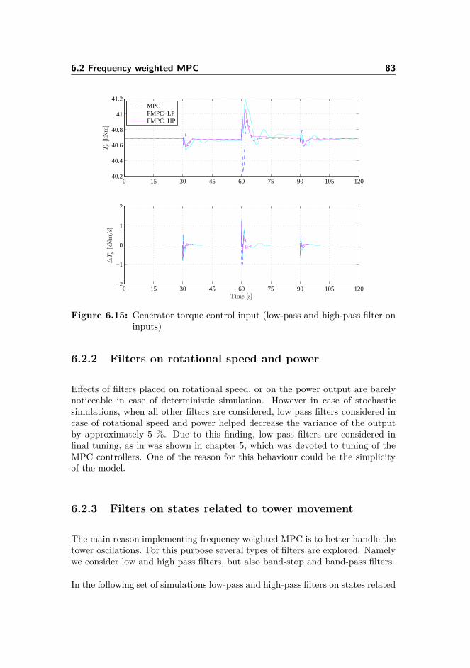
6.2 Frequency weighted MPC 83
0 15 30 45 60 75 90 105 12040.2
40.4
40.6
40.8
41
41.2Tg[kNm]
MPCFMPC−LPFMPC−HP
0 15 30 45 60 75 90 105 120−2
−1
0
1
2
△Tg[kNm/s]
Time [s]
Figure 6.15: Generator torque control input (low-pass and high-pass filter oninputs)
6.2.2 Filters on rotational speed and power
Effects of filters placed on rotational speed, or on the power output are barelynoticeable in case of deterministic simulation. However in case of stochasticsimulations, when all other filters are considered, low pass filters considered incase of rotational speed and power helped decrease the variance of the outputby approximately 5 %. Due to this finding, low pass filters are considered infinal tuning, as in was shown in chapter 5, which was devoted to tuning of theMPC controllers. One of the reason for this behaviour could be the simplicityof the model.
6.2.3 Filters on states related to tower movement
The main reason implementing frequency weighted MPC is to better handle thetower oscilations. For this purpose several types of filters are explored. Namelywe consider low and high pass filters, but also band-stop and band-pass filters.
In the following set of simulations low-pass and high-pass filters on states related

84 Full Load Simulations
to tower are considered (fig. 6.16). On the figure 6.17 we can see the effects onthe measurements, and tower displacement. Comparison with standard MPC isalso shown, so we can see the benefits of frequency tuning.
Low-pass filter, with frequency response shown on figure 6.16(a):
HLP (s) =1
4s + 1(6.3)
High-pass filter, with frequency response shown on figure 6.16(b):
HHP (s) =8s + 14s + 1
(6.4)
−40
−35
−30
−25
−20
−15
−10
−5
0
Mag
nitu
de (
dB)
10−2
10−1
100
101
−90
−45
0
Pha
se (
deg)
Bode Diagram
Frequency (rad/s)
(a) Low-pass filter
0
1
2
3
4
5
6
7
8
Mag
nitu
de (
dB)
10−2
10−1
100
101
0
5
10
15
20
Pha
se (
deg)
Bode Diagram
Frequency (rad/s)
(b) High-pass filter
Figure 6.16: Frequency response of considered filters
Low-pass filter in this case has negative effect on the overall performance. Powerand rotational speed is kept at theirs respective nominal values (fig. 6.17), whileusing low-pass filter, however the performance of the tower component is notsatisfactory (fig. 6.18). Cyan lines are used to display performance with low-pass filter. On the other hand high pass filter introduce some minor offsets inmeasured power and speed of the turbine, but oscillations of the tower relatedstates are significantly damped (magenta lines). The dashed (blue lines) showsperformance using standard MPC control. Using FMPC with high-pass filterwe can see improvement in contrast with MPC.Figures 6.19 and 6.20 shows thecontrol inputs. We may notice, that in case of low-pass filter, oscillations occursin the generator torque activity. This is cause by placing high weights in Qmatrix for rotational speed and generated power in FMPC design. Constraintson pitch rate are active only when high pass filter is used. Generator torquerate is way below it’s bounds in all cases. This is expectable, because the steadystate values of generator torque does not change in top region.

6.2 Frequency weighted MPC 85
0 15 30 45 60 75 90 105 1204.9
5
5.1Pe[M
W]
ReferenceMPCFMPC−LPFMPC−HP
0 15 30 45 60 75 90 105 12011.8
12.1
12.4
ωr[rpm]
Time [s]
Figure 6.17: Measurements - Pe and ωr (low-pass and high-pass filter on towerstates)
0 15 30 45 60 75 90 105 1200.15
0.25
0.35
xt[m
]
MPCFMPC−LPFMPC−HP
0 15 30 45 60 75 90 105 120−0.2
0
0.2
xt[m
/s]
Time [s]
Figure 6.18: Tower for-aft movement (low-pass and high-pass filter on towerstates)

86 Full Load Simulations
0 15 30 45 60 75 90 105 1209
10
11
12
13
14
15
β[deg]
MPCFMPC−LPFMPC−HP
0 15 30 45 60 75 90 105 120−10−8
−4
0
4
810
△β
[deg/s]
Time [s]
Figure 6.19: Pitch control inputs (low-pass and high-pass filter on towerstates)
0 15 30 45 60 75 90 105 1204.02
4.04
4.06
4.08
4.1
4.12
4.14x 10
4
Tg[kNm]
MPCFMPC-LPFMPC-HP
0 15 30 45 60 75 90 105 120−2
−1
0
1
2
△Tg[kNm/s]
Time [s]
Figure 6.20: Generator torque control input (low-pass and high-pass filter ontower states)
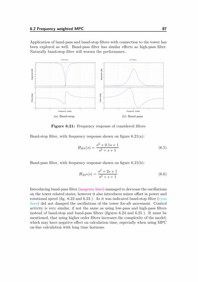
6.2 Frequency weighted MPC 87
Application of band-pass and band-stop filters with connection to the tower hasbeen explored as well. Band-pass filter has similar effects as high-pass filter.Naturally band-stop filter will worsen the performance..
−20
−18
−16
−14
−12
−10
−8
−6
−4
−2
0
Mag
nitu
de (
dB)
10−2
10−1
100
101
102
−90
−45
0
45
90
Pha
se (
deg)
Bode Diagram
Frequency (rad/s)
(a) Band-stop
0
1
2
3
4
5
6
7
8
Mag
nitu
de (
dB)
10−2
10−1
100
101
102
−20
−10
0
10
20
Pha
se (
deg)
Bode Diagram
Frequency (rad/s)
(b) Band-pass
Figure 6.21: Frequency response of considered filters
Band-stop filter, with frequency response shown on figure 6.21(a):
HBS(s) =s2 + 0.1s + 1
s2 + s + 1(6.5)
Band-pass filter, with frequency response shown on figure 6.21(b):
HBP (s) =s2 + 2s + 1s2 + s + 1
(6.6)
Introducing band-pass filter (magenta lines) managed to decrease the oscillationson the tower related states, however it also introduces minor offset in power androtational speed (fig. 6.22 and 6.23 ). As it was indicated band-stop filter (cyanlines) did not damped the oscillations of the tower for-aft movement. Controlactivity is very similar, if not the same as using low-pass and high-pass filtersinstead of band-stop and band-pass filters (figures 6.24 and 6.25 ). It must bementioned, that using higher order filters increases the complexity of the model,which may have negative effect on calculation time, especially when using MPCon-line calculation with long time horizons.
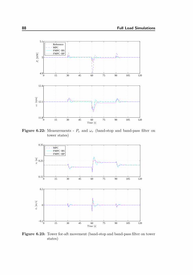
88 Full Load Simulations
0 15 30 45 60 75 90 105 1204.9
5
5.1
Pe[M
W]
ReferenceMPCFMPC−BSFMPC−BP
0 15 30 45 60 75 90 105 12011.8
12.1
12.4
ωr[rpm]
Time [s]
Figure 6.22: Measurements - Pe and ωr (band-stop and band-pass filter ontower states)
0 15 30 45 60 75 90 105 1200.15
0.25
0.35
xt[m
]
MPCFMPC−BSFMPC−BP
0 15 30 45 60 75 90 105 120−0.2
0
0.2
xt[m
/s]
Time [s]
Figure 6.23: Tower for-aft movement (band-stop and band-pass filter on towerstates)
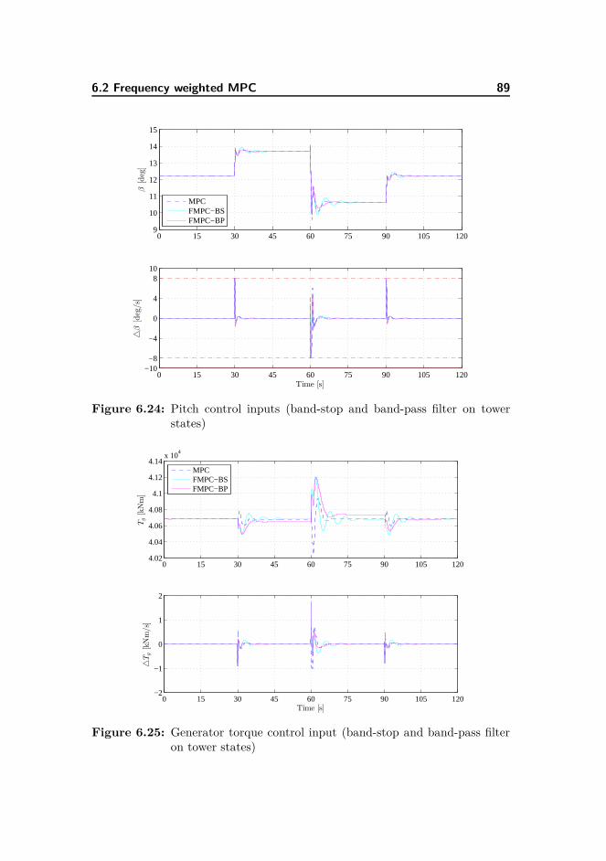
6.2 Frequency weighted MPC 89
0 15 30 45 60 75 90 105 1209
10
11
12
13
14
15β
[deg]
MPCFMPC−BSFMPC−BP
0 15 30 45 60 75 90 105 120−10−8
−4
0
4
810
△β
[deg/s]
Time [s]
Figure 6.24: Pitch control inputs (band-stop and band-pass filter on towerstates)
0 15 30 45 60 75 90 105 1204.02
4.04
4.06
4.08
4.1
4.12
4.14x 10
4
Tg[kNm]
MPCFMPC−BSFMPC−BP
0 15 30 45 60 75 90 105 120−2
−1
0
1
2
△Tg[kNm/s]
Time [s]
Figure 6.25: Generator torque control input (band-stop and band-pass filteron tower states)

90 Full Load Simulations
6.2.4 Final tuning
Stochastic simulation has been performed with final tuning presented in chapter5. As it was mentioned, low-pass filters are used on power output and measure-ment of the rotational speed, band-pass filters are considered on tower for-aftmovement and high-pass filters are applied on control inputs. Wind speed profileapplied to the system was shown in previous section (fig. 6.6).
Results are shown on following sets of figures. Comparison with standard MPCis made as well. Figure 6.26 shows the measurement of the rotational speedtogether with power generation. Notice slight increase in the variance of therotational speed against standard MPC controller. On figure 6.27 notice, thattower oscilations are much more damped using FMPC controller than usingstandard MPC. Pitch control activity of FMPC is very similar to standardMPC (fig. 6.28), but high frequency activity is removed from generator torquecontrol input (fig. 6.29). Such tuning on the generator torque action has beenchosen due to the fact, that gearbox and drive train (which are not consideredin this project) are very sensitive to high frequency changes in generator torquecontrol activity. Last figure shows cumulative sum of control rates, often namedas pitch travel (fig. 6.30). Slopes of pitch travel are very similar using bothMPC and FMPC, but there is huge difference in slopes of cumulative sum ofgenerator torque rate.
0 20 40 60 80 100 1204.95
5
5.05
Pow
er[M
W]
ReferenceMPCFMPC
0 20 40 60 80 100 12012
12.1
12.2
ωr[rpm]
Time [s]
ReferenceMPCFMPC
Figure 6.26: Measurements - Pe and ωr (final tuning)

6.2 Frequency weighted MPC 91
0 20 40 60 80 100 1200.16
0.18
0.2
0.22x
t[m
]
MPCFMPC
0 20 40 60 80 100 120−0.02
−0.01
0
0.01
0.02
xt[m
/s]
Time [s]
MPCFMPC
Figure 6.27: Tower for-aft movement (final tuning)
0 20 40 60 80 100 12014
16
18
20
22
Pitch
[deg]
MPCFMPC
0 20 40 60 80 100 120−1
−0.8
−0.4
0
0.4
0.81
Pitch
rate
[deg
per
sample]
Time [s]
MPCFMPC
Figure 6.28: Pitch control inputs (final tuning)

92 Full Load Simulations
0 20 40 60 80 100 1204.05
4.055
4.06
4.065
4.07
4.075
4.08x 10
4
Gen
eratorTorque[N
m] MPC
FMPC
0 20 40 60 80 100 120−200
−100
0
100
200
Torqu
erate
[Nm
per
sample]
Time [s]
MPCFMPC
Figure 6.29: Generator torque control input (final tuning)
0 20 40 60 80 100 1200
20
40
60
80
Pitch
Travel
MPCFMPC
0 20 40 60 80 100 1200
2000
4000
6000
8000
Time [s]
TorqueTravel
MPCFMPC
Figure 6.30: Cumulative sum of control moves (final tuning)

Chapter 7
Partial Load Simulations
In previous chapter attention was drawn to top region simulations. In this chap-ter the focus will be on partial load simulations (first three regions). Simulationsare performed in each region separately. Stochastic simulations are performedbetween regions, so region switching is demonstrated. An overall simulations inall four regions is shown at the end of the chapter.
7.1 WT0 model
Since controlling the wind turbine, is not a standard control problem, deter-ministic simulations with WT0 model are made. Behaviour of the system willbe demonstrated without any interference from tower for-aft movement or fromstochastic influences in the wind speed.
7.1.1 Simulations in R-I
The objective of the controller in the region number 1, is to maintain the ro-tational speed at it’s minimum speed, which is 6.9 rpm. Generated electricalpower Pe is maximized. Wind speed profile applied to this system is shown on
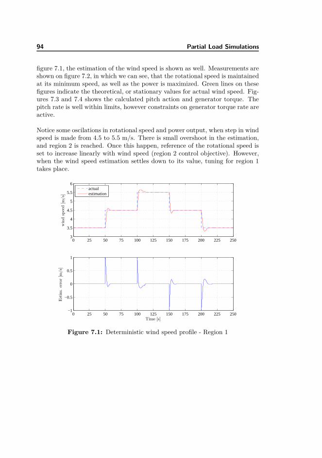
94 Partial Load Simulations
figure 7.1, the estimation of the wind speed is shown as well. Measurements areshown on figure 7.2, in which we can see, that the rotational speed is maintainedat its minimum speed, as well as the power is maximized. Green lines on thesefigures indicate the theoretical, or stationary values for actual wind speed. Fig-ures 7.3 and 7.4 shows the calculated pitch action and generator torque. Thepitch rate is well within limits, however constraints on generator torque rate areactive.
Notice some oscilations in rotational speed and power output, when step in windspeed is made from 4.5 to 5.5 m/s. There is small overshoot in the estimation,and region 2 is reached. Once this happen, reference of the rotational speed isset to increase linearly with wind speed (region 2 control objective). However,when the wind speed estimation settles down to its value, tuning for region 1takes place.
0 25 50 75 100 125 150 175 200 225 2503
3.5
4
4.5
5
5.5
6
windspeed[m
/s]
actualestimation
0 25 50 75 100 125 150 175 200 225 250−1
−0.5
0
0.5
1
Estim
.error[m
/s]
Time [s]
Figure 7.1: Deterministic wind speed profile - Region 1
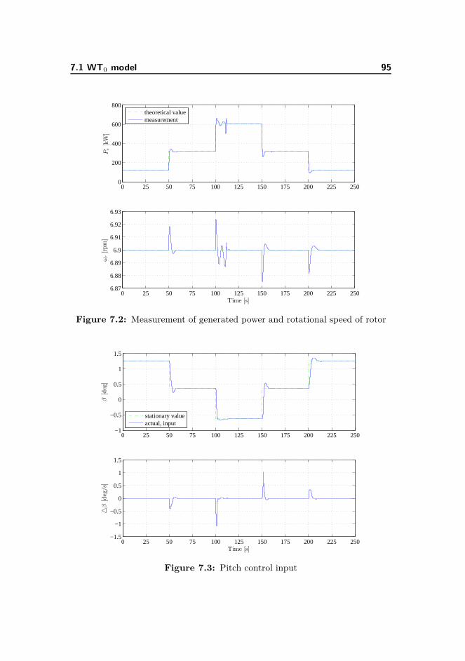
7.1 WT0 model 95
0 25 50 75 100 125 150 175 200 225 2500
200
400
600
800Pe[kW]
theoretical valuemeasurement
0 25 50 75 100 125 150 175 200 225 2506.87
6.88
6.89
6.9
6.91
6.92
6.93
ωr[rpm]
Time [s]
Figure 7.2: Measurement of generated power and rotational speed of rotor
0 25 50 75 100 125 150 175 200 225 250−1
−0.5
0
0.5
1
1.5
β[deg]
stationary valueactual, input
0 25 50 75 100 125 150 175 200 225 250−1.5
−1
−0.5
0
0.5
1
1.5
△β
[deg/s]
Time [s]
Figure 7.3: Pitch control input

96 Partial Load Simulations
0 25 50 75 100 125 150 175 200 225 2500
2
4
6
8
10Tg[kNm]
stationary valueactual input
0 25 50 75 100 125 150 175 200 225 250−20
−15
0
15
20
△Tg[kNm/s]
Time [s]
Figure 7.4: Generator torque control input
7.1.2 Simulations in R-II
In case of region number 2, main task is still to maximize power output, but therotational speed isn’t fixed like in region 1, but rise linearly with wind speed.This is achieved by setting the reference to the MPC based on wind speedestimation. Measurements are shown on figure 7.6. Notice power drops, whenwind speed increases. Justification for this behaviour lies in formerly mentioneddifferential equation 7.1, which describes the changes in angular velocity of therotor. From this we can understand, that if the wind speed increases, andthe rotor speed must increase accordingly, generator action must be lowered7.8. After such control action the kinetic energy of the wind will acceleratethe rotor. Steady state value for the entire mid region for the pitch valueis constant β ≈ −0.68 deg, but in order to make the power extraction moreefficient, calculations for the pitch angle are made as well (this was explained inrefch:hawt). Pitch control action is shown in figure 7.7, followed by generatortorque input 7.8.
Jωr =Pr
ωr
− NTg (7.1)
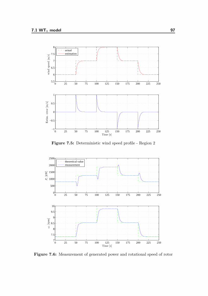
7.1 WT0 model 97
0 25 50 75 100 125 150 175 200 225 2505.5
6
6.5
7
7.5
8windspeed[m
/s]
actualestimation
0 25 50 75 100 125 150 175 200 225 250−1
−0.5
0
0.5
1
Estim
.error[m
/s]
Time [s]
Figure 7.5: Deterministic wind speed profile - Region 2
0 25 50 75 100 125 150 175 200 225 2500
500
1000
1500
2000
2500
Pe[kW]
theoretical valuemeasurement
0 25 50 75 100 125 150 175 200 225 2507
7.5
8
8.5
9
9.5
10
ωr[rpm]
Time [s]
Figure 7.6: Measurement of generated power and rotational speed of rotor
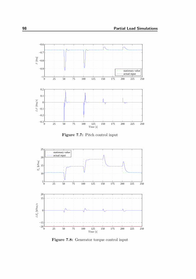
98 Partial Load Simulations
0 25 50 75 100 125 150 175 200 225 250−1
−0.9
−0.8
−0.7
−0.6
β[deg]
stationary valueactual input
0 25 50 75 100 125 150 175 200 225 250−0.3
−0.2
−0.1
0
0.1
0.2
△β
[deg/s]
Time [s]
Figure 7.7: Pitch control input
0 25 50 75 100 125 150 175 200 225 2505
10
15
20
25
Tg[kNm]
stationary valueactual input
0 25 50 75 100 125 150 175 200 225 250−20
−15
0
15
20
△Tg[kNm/s
Time [s]
Figure 7.8: Generator torque control input
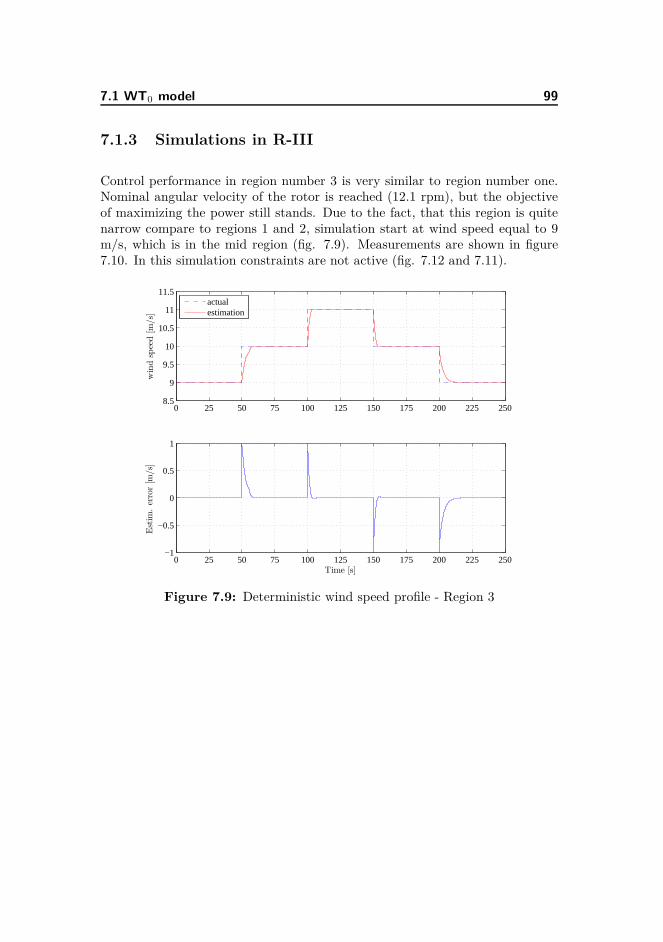
7.1 WT0 model 99
7.1.3 Simulations in R-III
Control performance in region number 3 is very similar to region number one.Nominal angular velocity of the rotor is reached (12.1 rpm), but the objectiveof maximizing the power still stands. Due to the fact, that this region is quitenarrow compare to regions 1 and 2, simulation start at wind speed equal to 9m/s, which is in the mid region (fig. 7.9). Measurements are shown in figure7.10. In this simulation constraints are not active (fig. 7.12 and 7.11).
0 25 50 75 100 125 150 175 200 225 2508.5
9
9.5
10
10.5
11
11.5
windspeed[m
/s]
actualestimation
0 25 50 75 100 125 150 175 200 225 250−1
−0.5
0
0.5
1
Estim
.error[m
/s]
Time [s]
Figure 7.9: Deterministic wind speed profile - Region 3

100 Partial Load Simulations
0 25 50 75 100 125 150 175 200 225 2502500
3000
3500
4000
4500
5000
5500
Pe[kW]
theoretical valuemeasurement
0 25 50 75 100 125 150 175 200 225 25010.5
11
11.5
12
12.5
ωr[rpm]
Time [s]
Figure 7.10: Measurement of generated power and rotational speed of rotor
0 25 50 75 100 125 150 175 200 225 250−1.6
−1.4
−1.2
−1
−0.8
−0.6
β[deg]
stationary valueactual input
0 25 50 75 100 125 150 175 200 225 250−0.1
−0.05
0
0.05
0.1
△β
[deg
per
sample]
Figure 7.11: Pitch control input
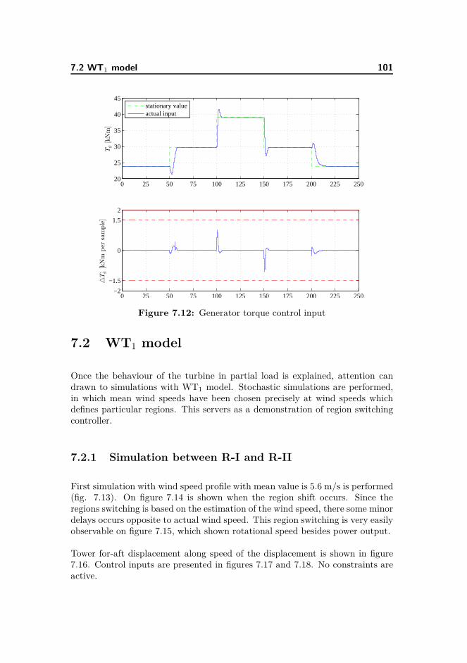
7.2 WT1 model 101
0 25 50 75 100 125 150 175 200 225 25020
25
30
35
40
45Tg[kNm]
stationary valueactual input
0 25 50 75 100 125 150 175 200 225 250−2
−1.5
0
1.5
2
△Tg[kNm
per
sample]
Figure 7.12: Generator torque control input
7.2 WT1 model
Once the behaviour of the turbine in partial load is explained, attention candrawn to simulations with WT1 model. Stochastic simulations are performed,in which mean wind speeds have been chosen precisely at wind speeds whichdefines particular regions. This servers as a demonstration of region switchingcontroller.
7.2.1 Simulation between R-I and R-II
First simulation with wind speed profile with mean value is 5.6 m/s is performed(fig. 7.13). On figure 7.14 is shown when the region shift occurs. Since theregions switching is based on the estimation of the wind speed, there some minordelays occurs opposite to actual wind speed. This region switching is very easilyobservable on figure 7.15, which shown rotational speed besides power output.
Tower for-aft displacement along speed of the displacement is shown in figure7.16. Control inputs are presented in figures 7.17 and 7.18. No constraints areactive.

102 Partial Load Simulations
0 25 50 75 100 125 150 175 200 225 2505
5.5
6
6.5
windspeed[m
/s]
actualestimation
0 25 50 75 100 125 150 175 200 225 250−0.2
−0.1
0
0.1
0.2
Estim
.error[m
/s]
Time [s]
Figure 7.13: Stochastic wind profile R-I/II
0 25 50 75 100 125 150 175 200 225 2501
2
3
4
Time [s]
region
actualbased on estimation
Figure 7.14: Region switching in partial load
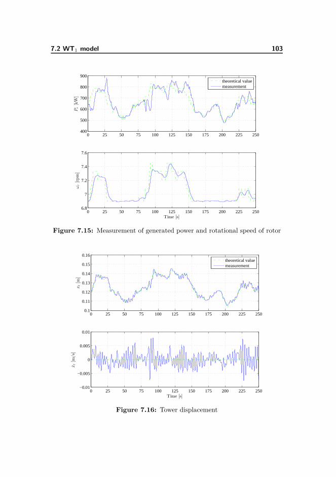
7.2 WT1 model 103
0 25 50 75 100 125 150 175 200 225 250400
500
600
700
800
900Pe[kW]
theoretical valuemeasurement
0 25 50 75 100 125 150 175 200 225 2506.8
7
7.2
7.4
7.6
ωr[rpm]
Time [s]
Figure 7.15: Measurement of generated power and rotational speed of rotor
0 25 50 75 100 125 150 175 200 225 2500.1
0.11
0.12
0.13
0.14
0.15
0.16
xt[m
]
theoretical valuemeasurement
0 25 50 75 100 125 150 175 200 225 250−0.01
−0.005
0
0.005
0.01
xt[m
/s]
Time [s]
Figure 7.16: Tower displacement
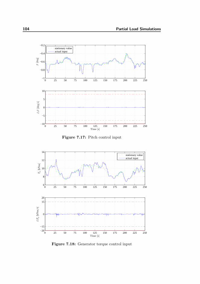
104 Partial Load Simulations
0 25 50 75 100 125 150 175 200 225 250−1
−0.8
−0.6
−0.4
−0.2
β[deg]
stationary valueactual input
0 25 50 75 100 125 150 175 200 225 250−10
−5
0
5
10
△β
[deg/s]
Time [s]
Figure 7.17: Pitch control input
0 25 50 75 100 125 150 175 200 225 2506
8
10
12
14
Tg[kNm]
stationary valueactual input
0 25 50 75 100 125 150 175 200 225 250−20
−15
0
15
20
△Tg[kNm/s]
Time [s]
Figure 7.18: Generator torque control input

7.2 WT1 model 105
7.2.2 Simulation between R-II and R-III
Stochastic wind speed profile with mean value of 10 m/s has been generated inorder to perform simulation between region 2 and 3 (fig. 7.20). Notice, increasedvariance of the noise. Region switching is shown on figure 7.19. Since the regionnumber 3 is narrow, and due to the increased variance of the noise, region 4 isreached for brief period of time.
0 25 50 75 100 125 150 175 200 225 2501
2
3
4
Time [s]
region
actualbased on estimation
Figure 7.19: Region switching in partial load
Notice similar behaviour in the rotational speed, like in previous sets of sim-ulations. In the R-III the rotational speed is kept at its nominal value, butwhen falling down to region 2, reference for the ωr is set according to wind seedestimation (fig. 7.21). At time instances, when region is switched from R-IIto R-III, power drops occurs. Reason for this is, that rather high weightingfactor is placed on the ωr control, and once the rotor is accelerated to nominalvalue, generator torque action (fig. 7.24) must be lowered for short time, soangular speed of 12.1 rpm can be maintained. Pitch values (fig. 7.23) are againcalculated, so power output is maximized.
Tower for-aft movement is presented in figure 7.22.

106 Partial Load Simulations
0 25 50 75 100 125 150 175 200 225 2508.5
9
9.5
10
10.5
11
11.5
windspeed[m
/s]
actualestimation
0 25 50 75 100 125 150 175 200 225 250−0.4
−0.2
0
0.2
0.4
Estim
.error[m
/s]
Time [s]
Figure 7.20: Stochastic wind profile R-II/III
0 25 50 75 100 125 150 175 200 225 2502000
3000
4000
5000
6000
Pe[kW]
theoretical valuemeasurement
0 25 50 75 100 125 150 175 200 225 25010.5
11
11.5
12
12.5
ωr[rpm]
Time [s]
Figure 7.21: Measurement of generated power and rotational speed of rotor
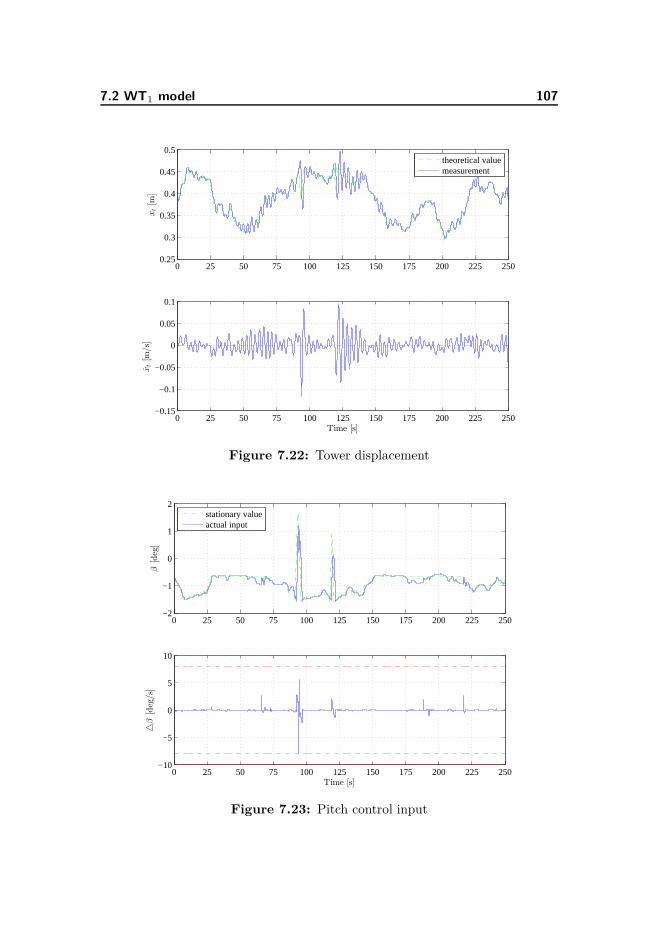
7.2 WT1 model 107
0 25 50 75 100 125 150 175 200 225 2500.25
0.3
0.35
0.4
0.45
0.5xt[m
]theoretical valuemeasurement
0 25 50 75 100 125 150 175 200 225 250−0.15
−0.1
−0.05
0
0.05
0.1
xt[m
/s]
Time [s]
Figure 7.22: Tower displacement
0 25 50 75 100 125 150 175 200 225 250−2
−1
0
1
2
β[deg]
stationary valueactual input
0 25 50 75 100 125 150 175 200 225 250−10
−5
0
5
10
△β
[deg/s]
Time [s]
Figure 7.23: Pitch control input
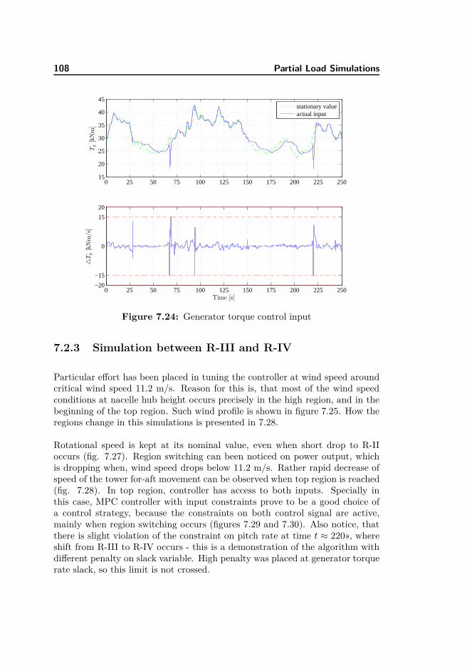
108 Partial Load Simulations
0 25 50 75 100 125 150 175 200 225 25015
20
25
30
35
40
45Tg[kNm]
stationary valueactual input
0 25 50 75 100 125 150 175 200 225 250−20
−15
0
15
20
△Tg[kNm/s]
Time [s]
Figure 7.24: Generator torque control input
7.2.3 Simulation between R-III and R-IV
Particular effort has been placed in tuning the controller at wind speed aroundcritical wind speed 11.2 m/s. Reason for this is, that most of the wind speedconditions at nacelle hub height occurs precisely in the high region, and in thebeginning of the top region. Such wind profile is shown in figure 7.25. How theregions change in this simulations is presented in 7.28.
Rotational speed is kept at its nominal value, even when short drop to R-IIoccurs (fig. 7.27). Region switching can been noticed on power output, whichis dropping when, wind speed drops below 11.2 m/s. Rather rapid decrease ofspeed of the tower for-aft movement can be observed when top region is reached(fig. 7.28). In top region, controller has access to both inputs. Specially inthis case, MPC controller with input constraints prove to be a good choice ofa control strategy, because the constraints on both control signal are active,mainly when region switching occurs (figures 7.29 and 7.30). Also notice, thatthere is slight violation of the constraint on pitch rate at time t ≈ 220s, whereshift from R-III to R-IV occurs - this is a demonstration of the algorithm withdifferent penalty on slack variable. High penalty was placed at generator torquerate slack, so this limit is not crossed.
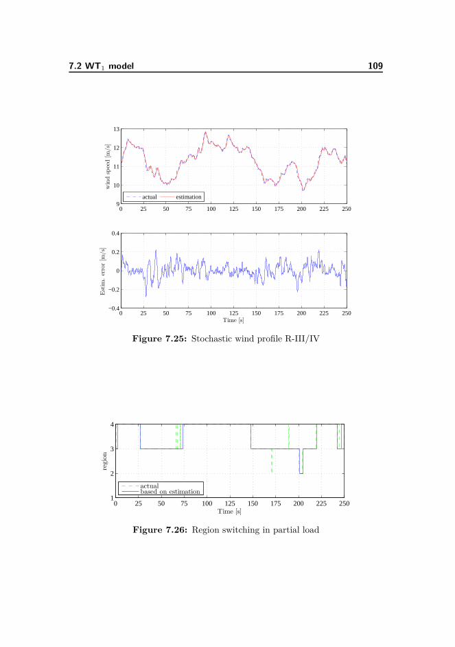
7.2 WT1 model 109
0 25 50 75 100 125 150 175 200 225 2509
10
11
12
13
windspeed[m
/s]
actual estimation
0 25 50 75 100 125 150 175 200 225 250−0.4
−0.2
0
0.2
0.4
Estim
.error[m
/s]
Time [s]
Figure 7.25: Stochastic wind profile R-III/IV
0 25 50 75 100 125 150 175 200 225 2501
2
3
4
Time [s]
region
actualbased on estimation
Figure 7.26: Region switching in partial load
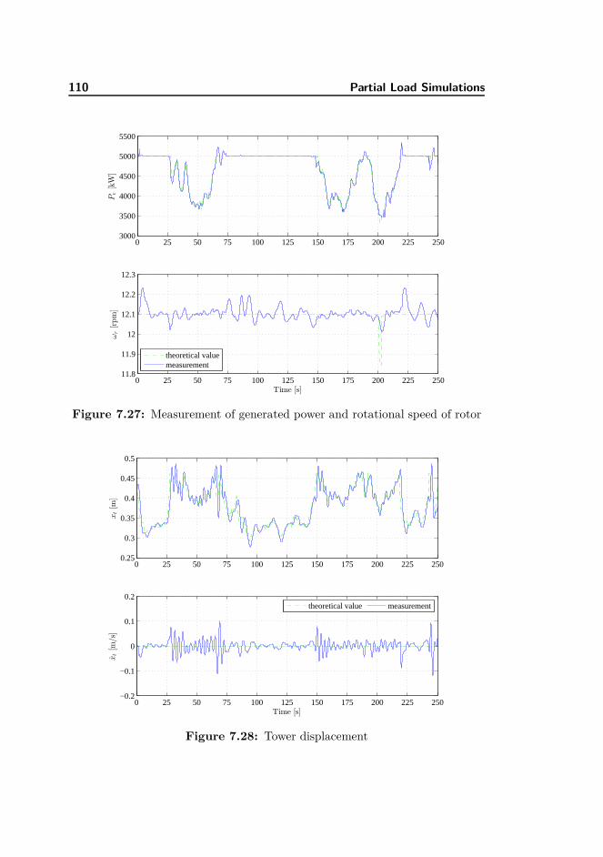
110 Partial Load Simulations
0 25 50 75 100 125 150 175 200 225 2503000
3500
4000
4500
5000
5500
Pe[kW]
0 25 50 75 100 125 150 175 200 225 25011.8
11.9
12
12.1
12.2
12.3
Time [s]
ωr[rpm]
theoretical valuemeasurement
Figure 7.27: Measurement of generated power and rotational speed of rotor
0 25 50 75 100 125 150 175 200 225 2500.25
0.3
0.35
0.4
0.45
0.5
xt[m
]
0 25 50 75 100 125 150 175 200 225 250−0.2
−0.1
0
0.1
0.2
xt[m
/s]
Time [s]
theoretical value measurement
Figure 7.28: Tower displacement
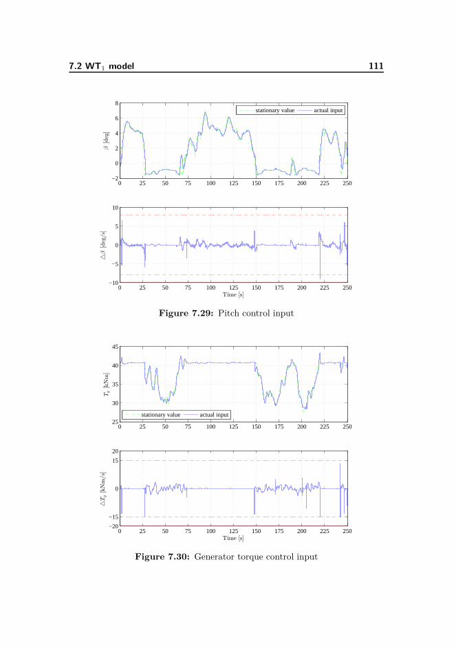
7.2 WT1 model 111
0 25 50 75 100 125 150 175 200 225 250−2
0
2
4
6
8β
[deg]
stationary value actual input
0 25 50 75 100 125 150 175 200 225 250−10
−5
0
5
10
△β
[deg/s]
Time [s]
Figure 7.29: Pitch control input
0 25 50 75 100 125 150 175 200 225 25025
30
35
40
45
Tg[kNm]
stationary value actual input
0 25 50 75 100 125 150 175 200 225 250−20
−15
0
15
20
△Tg[kNm/s]
Time [s]
Figure 7.30: Generator torque control input
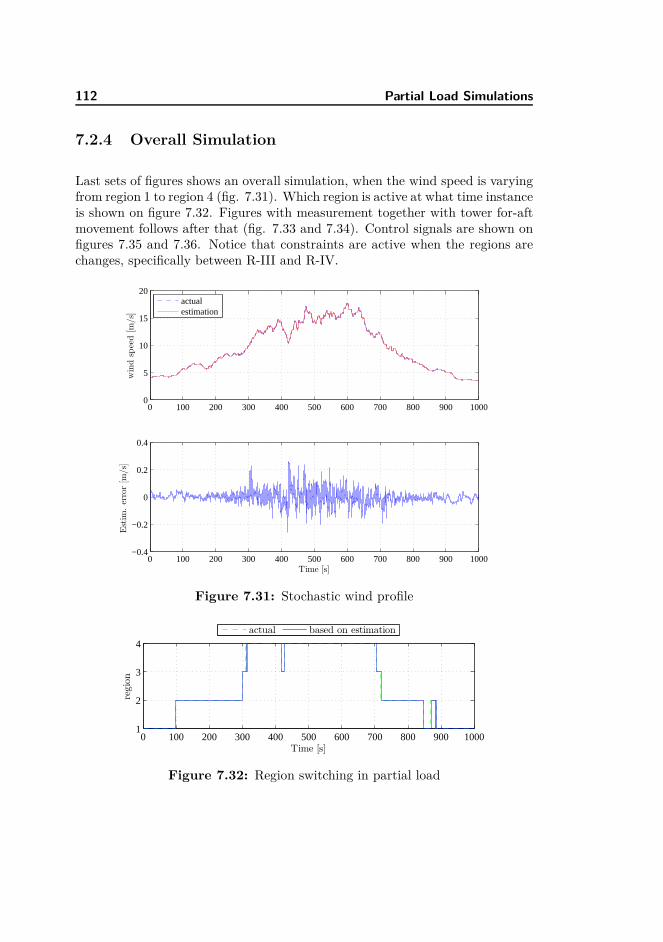
112 Partial Load Simulations
7.2.4 Overall Simulation
Last sets of figures shows an overall simulation, when the wind speed is varyingfrom region 1 to region 4 (fig. 7.31). Which region is active at what time instanceis shown on figure 7.32. Figures with measurement together with tower for-aftmovement follows after that (fig. 7.33 and 7.34). Control signals are shown onfigures 7.35 and 7.36. Notice that constraints are active when the regions arechanges, specifically between R-III and R-IV.
0 100 200 300 400 500 600 700 800 900 10000
5
10
15
20
windspeed[m
/s]
actualestimation
0 100 200 300 400 500 600 700 800 900 1000−0.4
−0.2
0
0.2
0.4
Estim
.error[m
/s]
Time [s]
Figure 7.31: Stochastic wind profile
0 100 200 300 400 500 600 700 800 900 10001
2
3
4
Time [s]
region
actual based on estimation
Figure 7.32: Region switching in partial load
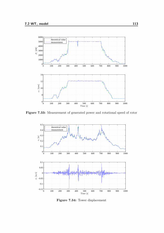
7.2 WT1 model 113
0 100 200 300 400 500 600 700 800 900 10000
1000
2000
3000
4000
5000
6000Pe[kW]
theoretical valuemeasurement
0 100 200 300 400 500 600 700 800 900 10006
8
10
12
14
ωr[rpm]
Time [s]
Figure 7.33: Measurement of generated power and rotational speed of rotor
0 100 200 300 400 500 600 700 800 900 10000
0.1
0.2
0.3
0.4
0.5
xt[m
]
theoretical valuemeasurement
0 100 200 300 400 500 600 700 800 900 1000−0.15
−0.1
−0.05
0
0.05
0.1
xt[m
/s]
Time [s]
Figure 7.34: Tower displacement

114 Partial Load Simulations
0 100 200 300 400 500 600 700 800 900 1000−5
0
5
10
15
β[deg]
stationary valueactual input
0 100 200 300 400 500 600 700 800 900 1000−10
−5
0
5
10
△β
[deg/s]
Time [s]
Figure 7.35: Pitch control input
0 100 200 300 400 500 600 700 800 900 10000
10
20
30
40
50
Tg[kNm]
stationary valueactual input
0 100 200 300 400 500 600 700 800 900 1000−20
−15
0
15
20
△Tg[kNm/s]
Time [s]
Figure 7.36: Generator torque control input

Chapter 8
Comparison of MPC Control
with Baseline Controller
In this chapter we will compare the results from previous simulations, usingMPC controllers, with currently implemented baseline PID controller. In thefirst section brief introduction to baseline controller will be given. The secondsection of this chapter is devoted into simulations and comparison of results.
8.1 Baseline Controller
This controller is implemented as a typical closed loop. The basic sketch of thesystem with the controller is shown on figure 8.1. The solely feedback input isthe generator speed or rotor speed. Low-pass measurement filter is introducedon the measurement so high frequency excitation is avoided.
The baseline controller has two main parts; table look-up for generator torque,and PI controller for collective pitch rate. Simple gain scheduling for the pro-portional and integral gain is implemented. Both control signals are saturatedif necessary, so the operational constraints are met. Contrary to the MPC de-sign presented in (chapter 5), where the minimum blade pitch is set to −5◦, incase of this PI controller, 0◦ is the minimum value. Further and more detailed

116 Comparison of MPC Control with Baseline Controller
information can be found in (Jonkman et al., 2009).
Figure 8.1: Sketch of baseline controller loop
8.2 Simulations with baseline controller
Baseline controller has been tested on same simulation model as MPC con-trollers. However, reader should keep in mind, that baseline controller presentedby (Jonkman et al., 2009) has been tuned for FAST system, which representsthe wind turbine much closely.
8.2.1 Full Load Simulations
Wind profile for the fourth region has been generated (fig. 8.2), and simulationwith this profile has been performed, so MPC strategies can be compared withthe baseline controller performance. Wind speed profile has been generated formean values equal to 18 m/s.
Figure 8.3 shows generated power Pe and rotational speed ωr. In both casesbaseline controller performs worse than MPC strategies, but within acceptable

8.2 Simulations with baseline controller 117
0 60 120 180 240 300 360 420 480 540 60010
15
20
25windspeed[m
/s]
Time [s]
Figure 8.2: Wind speed profile
margins. Second set of figures shows time evolution of states related to towerfor-aft movement (fig. 8.4). notice that tower oscillations are not damped usingbaseline controller. The speed of the tower displacement is gaining 10x highervalues compared to model predictive controllers.
0 60 120 180 240 300 360 420 480 540 6004.8
5
5.2
Pow
er[M
W]
Reference MPC FMPC PID
0 60 120 180 240 300 360 420 480 540 60011
11.5
12
12.5
13
13.5
ωr[rpm]
Time [s]
Figure 8.3: Measurements - Pe and ωr
Figure 8.5 show the pitch activity. Slow dynamics of the rotational speed,which is the solely input to the baseline controller, results in slow variations inpitch regulation. Model predictive controllers on the other hand counteract thevariations in wind speed much more aggressively. This behaviour of the pitchactivity also results in higher tower oscillations, because tower for-aft movement
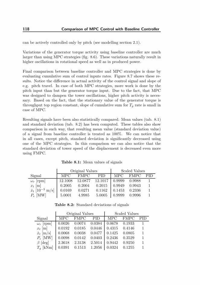
118 Comparison of MPC Control with Baseline Controller
can be actively controlled only by pitch (see modelling section 2.1).
Variations of the generator torque activity using baseline controller are muchlarger than using MPC strategies (fig. 8.6). These variations naturally result inhigher oscillations in rotational speed as well as in produced power.
Final comparison between baseline controller and MPC strategies is done byevaluating cumulative sum of control inputs rates. Figure 8.7 shows these re-sults. Notice the difference in actual activity of the control signal and slope ofe.g. pitch travel. In case of both MPC strategies, more work is done by thepitch input than but the generator torque input. Due to the fact, that MPCwas designed to dampen the tower oscillations, higher pitch activity is neces-sary. Based on the fact, that the stationary value of the generator torque isthroughput top region constant, slope of cumulative sum for Tg rate is small incase of MPC.
Resulting signals have been also statistically compared. Mean values (tab. 8.1)and standard deviation (tab. 8.2) has been computed. These tables also showcomparison in such way, that resulting mean value (standard deviation value)of a signal from baseline controller is treated as 100%. We can notice thatin all cases, except pitch, standard deviation is significantly decreased usingone of the MPC strategies. In this comparison we can also notice that thestandard deviation of tower speed of the displacement is decreased even moreusing FMPC.
Table 8.1: Mean values of signals
Original Values Scaled ValuesSignal MPC FMPC PID MPC FMPC PIDωr [rpm] 12.1008 12.0877 12.1017 0.9999 0.9988 1xt [m] 0.2005 0.2004 0.2015 0.9949 0.9943 1xt [10−3 m/s] 0.0169 0.0271 0.1162 0.1453 0.2336 1Pe [MW] 5.0001 4.9985 5.0005 0.9999 0.9996 1
Table 8.2: Standard deviations of signals
Original Values Scaled ValuesSignal MPC FMPC PID MPC FMPC PIDωr [rpm] 0.0026 0.0074 0.0384 0.0678 0.1933 1xt [m] 0.0192 0.0185 0.0446 0.4315 0.4146 1xt [m/s] 0.0068 0.0038 0.0477 0.1425 0.0805 1Pe [MW] 0.0098 0.0142 0.0403 0.2436 0.3529 1β [deg] 2.3618 2.3138 2.5014 0.9442 0.9250 1Tg [kNm] 0.0391 0.1513 1.2056 0.0324 0.1255 1

8.2 Simulations with baseline controller 119
0 60 120 180 240 300 360 420 480 540 6000
0.1
0.2
0.3
0.4xt[m
]MPC FMPC PID
0 60 120 180 240 300 360 420 480 540 600−0.15
−0.1
−0.05
0
0.05
0.1
0.15
xt[m
/s]
Time [s]
Figure 8.4: Tower displacement xt and speed of displacement xt
0 100 200 300 400 500 6005
10
15
20
25
β[deg]
MPC FMPC PID
0 60 120 180 240 300 360 420 480 540 600−10−8
−4
0
4
810
△β
[deg/s]
Time [s]
Figure 8.5: Pitch control action of baseline controller in full load
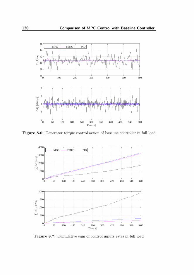
120 Comparison of MPC Control with Baseline Controller
0 100 200 300 400 500 60036
38
40
42
44
46
Tg[kNm]
MPC FMPC PID
0 60 120 180 240 300 360 420 480 540 600−2
−1
0
1
2
△Tg[kNm/s]
Time [s]
Figure 8.6: Generator torque control action of baseline controller in full load
0 60 120 180 240 300 360 420 480 540 6000
1000
2000
3000
4000
∑△β
[deg]
MPC FMPC PID
0 60 120 180 240 300 360 420 480 540 6000
500
1000
1500
2000
Time [s]
∑△Tg[kNm]
Figure 8.7: Cumulative sum of control inputs rates in full load

8.2 Simulations with baseline controller 121
8.2.2 Partial Load Simulations
Comparison between MPC strategies and baseline controller is done as well.Wind speed profile applied to the system is shown 8.8. There is little differencein power generation (fig. 8.9), despite the fact, that the baseline controller isnot pitching in the partial load (fig. 8.11). The trade of for this is, that therotational speed is kept above the theoretical values in R-II and below in R-I.In case of generator torque control action MPC is more active than baselinecontroller (fig. 8.12). This is also demonstrated in cumulative sums of controlrates (fig. 8.13).
0 100 200 300 400 500 6004
6
8
10
12
windspeed[m
/s]
Time [s]
Figure 8.8: Wind speed profile
0 60 120 180 240 300 360 420 480 540 6000
1
2
3
4
5
6
Pe[M
W]
Theoretical valueMPCPID
0 60 120 180 240 300 360 420 480 540 6006
8
10
12
14
ωr[rpm]
Time [s]
Figure 8.9: Measurements - Pe and ωr

122 Comparison of MPC Control with Baseline Controller
0 60 120 180 240 300 360 420 480 540 6000
0.1
0.2
0.3
0.4
0.5
xt[m
]
MPCPID
0 60 120 180 240 300 360 420 480 540 600−0.1
−0.05
0
0.05
0.1
xt[m
/s]
Time [s]
Figure 8.10: Tower displacement xt and speed of displacement xt
0 60 120 180 240 300 360 420 480 540 600−2
−1
0
1
2
β[deg]
MPC PID
0 60 120 180 240 300 360 420 480 540 600−10−8
−4
0
4
810
△β
[deg/s]
Time [s]
Figure 8.11: Pitch control action of baseline controller in partial load

8.2 Simulations with baseline controller 123
0 60 120 180 240 300 360 420 480 540 6000
10
20
30
40
50Tg[kNm]
MPCPID
0 60 120 180 240 300 360 420 480 540 600−20
−15
−7.5
0
7.5
15
20
△Tg[kNm/s]
Time [s]
Figure 8.12: Generator torque control action of baseline controller in partialload
0 100 200 300 400 500 6000
100
200
300
400
∑△β
[deg]
MPC PID
0 100 200 300 400 500 6000
1000
2000
3000
4000
Time [s]
∑△Tg[kNm]
Figure 8.13: Cumulative sum of control inputs rates in partial load

124 Comparison of MPC Control with Baseline Controller
Chapter 9
Conclusion & Perspectives
9.1 Conclusion
9.1.1 Theory and Methods
This project has been dealing with MPC control of the wind turbines. Before anycontroller can be designed, a mathematical model of the plant must be derived.In this project, third order system of the wind turbine has been considered.Since the controller proposed in this project is based on linear state space model,Taylor series expansion has been used to obtain LTI model.
Proposed MPC control with receding horizon policy is based on state feedback,thus state estimator must be used. Based on the facts, that wind speed measure-ment has not been considered, and that system dynamics change with increasingwind speed, wind speed must be estimated as well. Disturbance modelling hasbeen used for this purpose. Estimator in the form of a stationary predictiveKalman filter was designed. This estimator is then used to estimate the states,the wind speed and unmeasured disturbances.
In this project two alternative MPC strategies has been investigated. Firstlystandard MPC formulation, in which the tuning parameters are weighting matri-

126 Conclusion & Perspectives
ces. Secondly, frequency weighted MPC is considered, in which tuning is shiftedfrom weighting matrices to designing filters in form of transfer functions.
9.1.2 Simulations and Results
Multiple simulations have been performed. In order to understand system be-haviour at different wind speeds, deterministic wind profiles has been appliedto the system. Simulations with stochastic wind speed profiles has been used todemonstrate how the system performs in "closer to reality" conditions.
Objective in the partial load case was to maximize power output. It has beendemonstrated with satisfactory results, that MPC controller can fulfil this ob-jective. Region switching algorithm has been used, in order to control the rota-tional speed, thus maximizing the power output. Several approaches of controlhas been investigated in this case. Since MPC controller can not control the tur-bine with pitch action, pitch must be calculated separately. Best power outputhas been gained by algorithm, that calculates the pitch action in such way, thatmaximum cp value is found for given value of λ. Using this approach, rotationalspeed and power output has been kept closer to the stationary values.
In the full load case, where the objective is to control the power and rotationalspeed at its nominal values, two MPC controllers have been compared. BothMPC strategies yields satisfactory results. However, FMPC has proven to per-form better in dampening tower oscillations, thus decreasing the physical strainof the tower.
Finally comparison between MPC strategies and baseline controller was done.Differences in energy production between MPC and baseline controller is ex-tremely small. But if we take into consideration other objectives of the controllerlike damping tower oscilations, MPC strategies proven to do a better job.
9.2 Perspectives
In wind turbine control are many challenges, which were not addressed in thethis project.
In general, taking into account more complex models, like flexible drive shaft,or blade momentum could improve the overall performance of the wind turbinepower generation. Knowing the dynamics of the system also allows us to design

9.2 Perspectives 127
control strategies which address several issues i.e. decrease the structural fa-tigue, thus prolonging the lifetime of the entire wind turbine device. Proposedfrequency weighted MPC prove to suitable to tool for fulfilling those controlobjectives. This combines together the advantages of model predictive control,such as constraints handling, together with frequency weighting, which is suit-able for deceasing the physical stress on the tower. Since this approach has aform of gain scheduling, more precise estimation of the wind speed can prove toimprove the overall performance. For this purpose we might use time varyingKalman filter or extended non-linear Kalman filter.

128 Conclusion & Perspectives
Appendix A
System Parameters
A.1 Physical Parameters of Wind Turbine
Table A.1: Physical Parameters
Quantity Units ValueR m 63H m 90J kg.m2 38768000Mt kg 422780Dt N.m−1.s−1 20213Kt N.m−1 1654700
Constants Mt, Dt, Kt were taken from (Henriksen, 2007). Constants R, H , Jfrom (Jonkman et al., 2009).
A.2 Calculated Matrices and Transfer Functions
In this section are presented state spaces models at 7 and 15 m/s. Also unscaledand scaled models are presented.

130 System Parameters
Continuous State-Space model linearised at 7 m/s unscaled
A =
−0.0350 0 −0.01490 0 10.5818 −3.9139 −0.1844
(A.1a)
B =
0 −2.5 · 10−6
0 0−0.0515 0
(A.1b)
Bv =
0.014900.1366
(A.1c)
C =
1398998 0 01 0 00 0 1
(A.1d)
D =
0 86.82100 00 0
(A.1e)
Continuous State-Space model linearised at 7 m/s scaled
A =
−0.0350 0 −0.01490 0 10.5818 −3.9139 −0.1844
(A.2a)
B =
0 −0.11260 0
−1.1331 0
(A.2b)
Bv =
0.014900.1366
(A.2c)
C =
0.3205 0 01 0 00 0 1
(A.2d)
D =
0 0.89510 00 0
(A.2e)

A.2 Calculated Matrices and Transfer Functions 131
Continuous State-Space model linearised at 15 m/s unscaled
A =
−0.1362 0 −0.02630 0 1
−0.5836 −3.9139 −0.2223
(A.3a)
B =
0.0158 −2.5 · 10−6
0 0−0.1490 0
(A.3b)
Bv =
0.026300.1745
(A.3c)
C =
1398998 0 01 0 00 0 1
(A.3d)
D =
0 86.82100 00 0
(A.3e)
Continuous State-Space model linearised at 15 m/s scaled
A =
−0.1362 0 −0.02630 0 1
−0.5836 −3.9139 −0.2223
(A.4a)
B =
−0.3484 −0.11260 0
−3.2781 0
(A.4b)
Bv =
0.026300.1745
(A.4c)
C =
3945990 0 01 0 00 0 1
(A.4d)
D =
0 122.90960 00 0
(A.4e)

132 System Parameters

Appendix B
Detailed Frequency Responses
More detailed frequency responses are shown in this appendix. 3D bode plotsare made, so reader can see the evolution of magnitude and phase throughoutoperational wind speed interval. In all frequency responses we can see rapidchange in responses starting at critical wind speed 11.2 m/s. This is caused bythe fact, that we cannot control the linear model using pitch in the partial load,but only by generator torque.

134 Detailed Frequency Responses
35.6
1011.2
25
10−4
10−2
100
102
−200
−150
−100
−50
0
50
windspeed[m/s]
Frequency [rad/s]
Mag
nitude[dB]
35.6
1011.2
25
10−4
10−2
100
102
−150
−100
−50
0
50
windspeed[m/s]
Frequency [rad/s]
Mag
nitude[dB]
35.6
1011.2
25
10−4
10−2
100
102
−180
0
180
360
540
windspeed[m/s]
Frequency [rad/s]
Phase[deg]
(a) Gβ,Pe(jω)
35.6
1011.2
25
10−4
10−2
100
102
−180
0
180
360
540
windspeed[m/s]
Frequency [rad/s]
Phase[deg]
(b) Gβ,ωr(jω)
35.6
1011.2
25
10−4
10−2
100
102
−100
−50
0
50
windspeed[m/s]
Frequency [rad/s]
Mag
nitude[dB]
35.6
1011.2
25
10−4
10−2
100
102
−150
−100
−50
0
50
windspeed[m/s]
Frequency [rad/s]
Mag
nitude[dB]
35.6
1011.2
25
10−4
10−2
100
102
0
180
360
windspeed[m/s]
Frequency [rad/s]
Phase
[deg]
(c) Gβ,xt(jω)
35.6
1011.2
25
10−4
10−2
100
102
90
180
270
360
450
windspeed[m/s]
Frequency [rad/s]
Phase
[deg]
(d) Gβ,xt(jω)
Figure B.1: Frequency response of transfer functions from pitch control inputto outputs
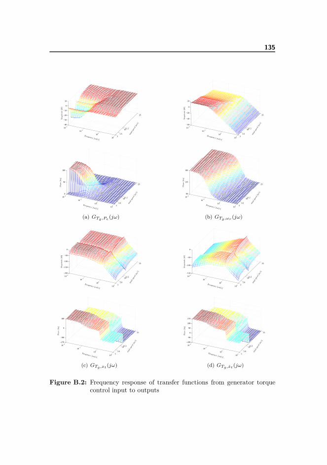
135
35.6
1011.2
25
10−4
10−2
100
102
−40
−30
−20
−10
0
10
windspeed[m/s]
Frequency [rad/s]
Magnitude[dB]
35.6
1011.2
25
10−4
10−2
100
102
−60
−40
−20
0
20
windspeed[m/s]
Frequency [rad/s]
Magnitude[dB]
35.6
1011.2
25
10−4
10−2
100
102
0
90
180
windspeed[m/s]
Frequency [rad/s]
Phase[deg]
(a) GTg ,Pe(jω)
35.6
1011.2
25
10−4
10−2
100
102
90
135
180
windspeed[m/s]
Frequency [rad/s]
Phase[deg]
(b) GTg ,ωr(jω)
35.6
1011.2
25
10−4
10−2
100
102
−200
−150
−100
−50
0
windspeed[m/s]
Frequency [rad/s]
Mag
nitude[dB]
35.6
1011.2
25
10−4
10−2
100
102
−150
−100
−50
0windspeed[m/s]
Frequency [rad/s]
Mag
nitude[dB]
35.6
1011.2
25
10−4
10−2
100
102
−270
−180
0
180
windspeed[m/s]
Frequency [rad/s]
Phase
[deg]
(c) GTg ,xt(jω)
35.6
1011.2
25
10−4
10−2
100
102
−180
−90
0
90
180
270
windspeed[m/s]
Frequency [rad/s]
Phase
[deg]
(d) GTg ,xt(jω)
Figure B.2: Frequency response of transfer functions from generator torquecontrol input to outputs
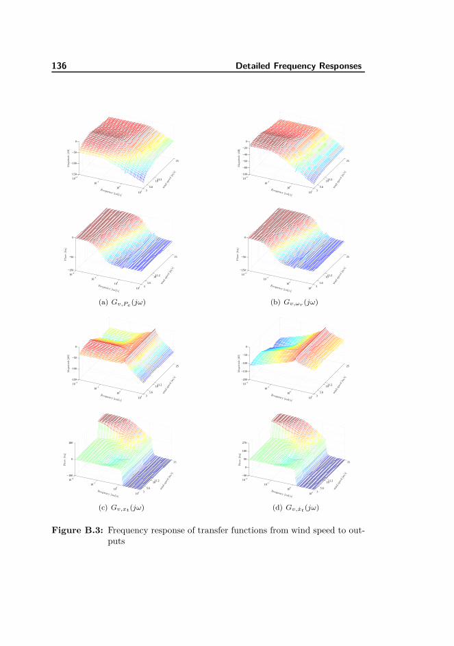
136 Detailed Frequency Responses
35.6
1011.2
25
10−4
10−2
100
102
−150
−100
−50
0
windspeed[m/s]
Frequency [rad/s]
Mag
nitude[dB]
35.6
1011.2
25
10−4
10−2
100
102
−100
−80
−60
−40
−20
0
windspeed[m/s]
Frequency [rad/s]
Mag
nitude[dB]
35.6
1011.2
25
10−4
10−2
100
102
−150
−90
0
windspeed[m/s]
Frequency [rad/s]
Phase[deg]
(a) Gv,Pe(jω)
35.6
1011.2
25
10−4
10−2
100
102
−150
−90
0
windspeed[m/s]
Frequency [rad/s]
Phase[deg]
(b) Gv,ωr (jω)
35.6
1011.2
25
10−4
10−2
100
102
−150
−100
−50
0
windspeed[m/s]
Frequency [rad/s]
Mag
nitude[dB]
35.6
1011.2
25
10−4
10−2
100
102
−200
−150
−100
−50
0
windspeed[m/s]
Frequency [rad/s]
Mag
nitude[dB]
35.6
1011.2
25
10−4
10−2
100
102
−180
0
180
windspeed[m/s]
Frequency [rad/s]
Phase
[deg]
(c) Gv,xt (jω)
35.6
1011.2
25
10−4
10−2
100
102
−90
0
90
180
270
windspeed[m/s]
Frequency [rad/s]
Phase
[deg]
(d) Gv,xt (jω)
Figure B.3: Frequency response of transfer functions from wind speed to out-puts
Bibliography
Ahmad, A. and Wahib, A. (2007). Application of Model Predictive Control(MPC) Tuning Strategy in Multivariable Control of Distillation Column.Reaktor, Vol. 11:66–70.
Åström, K. (1970). Introduction to Stochastic Control Theory. Dover Publica-tions, Inc., Mineola, New York.
Bendtsen, J., Trangbaek, K., and Stoustrup, J. (2010). Hierarchical modelpredictive control for resource distribution. In Decision and Control (CDC),2010 49th IEEE Conference on, pages 2468 –2473.
Bossanyi, E. A. (2003). Individual blade pitch control for load reduction. WindEnerg, 6:119–128.
Bourlis, D. and Bleijs, J. (2010). A wind speed estimation method using adap-tive Kalman filtering for a variable speed stall regulated wind turbine. InProbabilistic Methods Applied to Power Systems (PMAPS), 2010 IEEE 11thInternational Conference on, pages 89 –94.
Boyd, S. and Vandenberghe, L. (2009). Convex Optimization. Cambridge Uni-versity Press, New York, USA, 7th edition.
Brown, R. G. and Hwang, P. Y. C. (1997). Introduction to Random Signals andApplied Kalman Filtering, volume 2. John Wiley & Sons.
Burton, T., Shrape, D., Jenkins, N., and E., B. (2001). Wind Energy Handbook.J. Wiley.
Camacho, E. F. and Bordons, C. (2007). Model Predictive Control. Springer,2nd edition.
138 BIBLIOGRAPHY
Gosk, A. (2011). Model predictive control of a wind turbine. Master’s thesis,Denmark University of Technology.
Hansen, M. (2008). Aerodynamics of Wind Turbines. Earthscan.
Henriksen, L. C. (2007). Model predictive control of a wind turbine. Master’sthesis, Denmark University of Technology.
IEC-CDV (2004). WIND TURBINES CDV STANDARD. International Elec-trotechnical Commission, Geneva, Switzerland, 2nd revision edition.
J. Jonkman and Bir, G. (2007). Aeroelastic instabilities of large offshore andonshore wind turbines. Technical report, National Renewable Energy Labo-ratory, U.S.
Jonkman, J., Butterfield, S., Musial, W., and Scott, G. (2009). Definition ofa 5MW reference wind turbine for offshore system development. Technicalreport, National Renewable Energy Laboratory, U.S.
Jonkman, J. M. and Buhl Jr., M. L. (2005). FAST User’s Guide. NationalRenewable Energy Laboratory, USA.
Jørgensen, J. (2011). Model predictive control course. Lecture Notes.
Kalman, R. E. (1960). A new approach to linear filtering and prediction prob-lems. Transactions of the ASME–Journal of Basic Engineering, 82(SeriesD):35–45.
Kvasnica, M. (2009). Real-Time Model Predictive Control via Multi-ParametricProgramming: Theory and Tools. VDM Verlag, Saarbruecken.
Laks, J., Pao, L., and Wright, A. (2009). Control of wind turbines: Past,present, and future. In American Control Conference, 2009. ACC ’09., pages2096 –2103.
Larsson, M. (2004). A model-predictive approach to emergency voltage controlin electrical power systems. In Decision and Control, 2004. CDC. 43rd IEEEConference on, volume 2, pages 2016 – 2022 Vol.2.
Maciejowski, J. (2002). Predictive Control with Constraints. PEARSONPrentice-Hall.
Mancuso, G. M. and Kerrigan, E. C. (2011). Solving constrained LQR problemsby eliminating the inputs from the QP. In IEEE Conference on Decision andControl, Orlando, FL, USA.
Mirzaei, M., Henriksen, L. C., Poulsen, N. K., Niemann, H. H., and Hansen,M. H. (2012a). Individual pitch control using LIDAR measurements. In IEEEMulti-Conference on Systems and Control, Dubrovnik, Croatia.
BIBLIOGRAPHY 139
Mirzaei, M., Poulsen, N. K., and Niemann, H. H. (2012b). Robust Model Pre-dictive Control of a Wind Turbine. American Control Conference.
Muske, K. R. and Rawlings, J. (1993). Model predictive control with linearmodels. AIChE Journal, 39(2).
Nikolaou, M. (2001). Model Predictive Controllers: A Critical Synthesis ofTheory and Industrial Needs. Advances in Chemical Engineering, AcademicPress, Vol. 26:131–204.
Nocedal, J. and Wright, S. (1999). Numerical Optimization. Springer Series inOperations Research. Springer.
Østergaard, K. Z., Brath, P., and Stoustrup, J. (2007). Estimation of effectivewind speed. Journal of Physics: Conference Series 75.
Østergaard, K. Z., Stoustrup, J., and Brath, P. (2008). Linear parameter varyingcontrol of wind turbines covering both partial and full load considitons. InInternational Journal of Robust and Nonlinear Control, volume 19.
Pannocchia, G. and Rawlings, J. (2003). Disturbance models for offset-freemodel-predictive control. AIChE Journal, 49(2).
Poulsen, N. K. (2007). Stokastik Adaptiv Regulering. Informatik og MatematiskModellering, DTU.
Prasath, G. and Jørgensen, J. (2009). Soft constraints for robust MPC of Uncer-tain systems. In International Symposium on Advanced Control of ChemicalProcesses.
Prasath, G., Recke, B., Chidambaram, M., and Jørgensen, J. (2010). Applica-tion of Soft Constrained MPC to a Cement Mill Circuit. In Proceedings of the9th International Symposium on Dynamics and Control of Process Systems,Belgium, Leuven.
Primbs, J. (2007). A soft constraint approach to Stochastic Receding HorizonControl. In Decision and Control, 2007 46th IEEE Conference on, pages 4797–4802.
Skogestad, S. and Postlethwaite, I. (2005). Multivariable Feedback Control:Analysis And Design. John Wiley.
Wills, A. (2007). QPC - Quadratic Programming in C.http://sigpromu.org/quadprog/.
Xin, M. (1994). Modelling and control of a wind turbine. Master’s thesis,Denmark Univeristy of Technology.

140 BIBLIOGRAPHY
Xin, M., Poulsen, N., and Bindner, H. (1997). Estimation of the wind speedin connection to wind turbines. In Proceedings of the IASTED InternationConference CONTROL’97, Mexico, Cancun.
Zeilinger, M., Jones, C., and Morari, M. (2010). Robust stability propertiesof soft constrained mpc. In Decision and Control (CDC), 2010 49th IEEEConference on, pages 5276 –5282.


