Model reference adaptive control of dynamic output feedback linearisable systems with unknown high frequency g

Z. Ding

Abstract: The paper deals with model reference adaptive control of single-input/single-output nonlinear systems which are linearisable by dynamic output feedback. A class of systems discussed is specified by a set of coordinate-free geometric conditions. The systems are linear with respect to the input and unknown constant parameters. The nonlinear terms, in suitable coordinates, depend on the output only. When the parameters are known, the systems can be exactly linearised by dynamic output feedback. A key feature of the class of nonlinear systems considered in this paper is that no a priori information is assumed on the high frequency gain. A global adaptive control algorithm with a Nussbaum gain is proposed for the systems considered and is demonstrated by a physical example.

1 Introduction

Adaptive control of linear continuous systems has been successfully solved in the last decade [I, 21. The original algorithms [ 3 , 41 are proposed under four assumptions: (i) the known sign of the high frequency gain; (ii) the known relative degree; (iii) a known upper bound of the model order; and (iv) the minimum phase. Further developments are proceeding in a number of directions, including the generalisation to nonlinear systems, relax- ation on the assumptions and improvement in the robustness of adaptive control algorithms.

It is clear that there are some particular systems for which the sign of the high frequency gain is known a priori, or can be identified offline by introducing a high frequency probing signal into the system. However, the assumption on the knowledge of the high frequency gain does not generally appear to be practical. The problem, then, is to determine whether the known sign of the high frequency gain is necessary for adaptive control. It is pointed out that a controller with rational

IEE Proreedings online no. 19971491 0 IEE, 1997

Paper first received 13th January arid in revised fonn 30th June 1997 Thc author is with the Department of‘ Mechanical Engineering, Ngee Ann Polytechnic, 535 Cleinenti Road, Singapore 599489, Republic of Singapore

functions cannot stabilise a class of first order linear systems for some initial values [5]. A breakthrough, reported in 161, tells that there exists a class of smooth first order controllers to stabilise general first order sys- tems without a priori information on the high fre- quency gain. This success was achieved using an ‘irrational gain function’, sometimes referred to as the N ussbauin gain. This was quickly generalised to linear systems of relative degree p 5 2 [7, 81 and to linear sys- tems of p 2 1 [9].

Alternatively, differential geometry has been applied to analysis and control of nonlinear systems. It has been shown that some nonlinear systems can be trans- formed into linear or partly linear systems using state feedback or output feedback [lo]. The conditions for the existence of such a coordinate transform are often specified in a coordinate-free fashion. Adaptive control has been introduced to state feedback linearisable sys- tems when there are uncertainties in the parameters [ 1 1 , 121. Dynamic output feedback linearisation for systems with known parameters is presented in [13] using Gltered transforms. Adaptive control via output feedback for a more general class of nonlinear systems has been solved using backstepping together with fil- tered transforms 1141 or K-filters [15]. However, the above algorithms are all under the assumption that the sign of the high frequency gain is known. Adaptive control with unknown high frequency gain is intro- duced for first order nonlinear systems using the Nuss- baum gain [16]. An alternative method is developed through a modification to the parameter estimation algorithm [17]. In both the cases, the algorithms are limited to first order nonlinear systems.

In this paper we focus our attention on model refer- ence adaptive control of dynamic output-feedback line- arisable systems without a priori information on the sign of the high frequency gain. Coordinate-free geo- metric conditions are identified for the existence of a global transform to make nonlinear systems with unknown parameters linearisable through dynamic out- put feedback. Instead of the filtered transformation, the filters designed for linear adaptive systems [ I , 21 are used for the nonlinear terms depending on the output, as well as for the input ana ourput. A new model refer- ence adaptive control algorithm with a Nussbaum gain is proposed for the class of nonlinear systems consid- ered to achieve asymptotic output tracking.

421 ILX Proc.-Control Theory Appl.. Vol. 144, No. 5, September I997

2 Geometric conditions

A , =

A large class of nonlinear systems can be described by r P 1 P

- 0 1 0 . 0 0 0 1 ' 0 . . . . ~ . . . . . . . 0 0 0 ' . . 1 - 0 0 0 ' 0

L 2 = 1 1 2 = 1

Y = 145) (1) where 5 E R" is the state vector, U E R i s the control, 8 = [e , , ..., e,,]' is the constant uncertain parameter vector belonging to 52, a closed subset in RP, h. R" + R is the smooth output function, and f, go, g,, qi, 1 I z I p , are smooth vector fields in R", with go(<) z 0, V< E R". We assume, without 1 0 s of generality, that h(0) = 0 and that 8 = 0 is the nominal parameter.

In this paper we use some terminologies and nota- tions of differential geometry which are essential for the study of nonlinear systems and can be found in ref- erences 5uch ds [18, 191. The generalisations to nonlin- ear systems can be found in [lo] for control concepts, such as the relative degree, minimum phase, controlla- bility and observability In the following theorem, the coordinate-free geometric conditions are identified for the class of nonlinear systems considered in this paper. Theorem I Let the system (eqn 1) be of minimuin phase and of constant relative degree p, for all 6 E 52. Then the system is transformable by a state space diffe- omorphism, independent of 8,

into x = T(C), T(0) = 0, x E Rn ( 2 )

X = A,x + a(Q)y + b(Q)a(y)u 2)

z = 1

y = c,x ( 3 ) with cr: R - R, I$: R + Rn, 0 I i I p , (Ac, b, c , ) mini-

a(Q) =

7 h , (111 =

0

, C T =

&n(Y) for 0 I z I p , if and only if (1) rank{&, .., d(Lj+lh)} = n (ii) [a&, ad&] = 0, 0 I z, j 5 n - 1, (111) [q,, ud+z] = 0, 1 5 i 5 p , 0 I j I n - 2 (iv) there exist a smooth function o: R + R, and n -- p + 1 reals bp(S)m, ..., /I,(@, depending on parameter

428

vector 0, such that

z= 1 3=1

(v) the vector fields ad& 0 I i I n ~ 1, are complete, where z is the vector field satisfying

PruuJ The coordinate-free geometric conditions (i) to (v) are shown in theorem 7.4.1 in [20] and theorem 2.1 in [14] to be the necessary and sufficient conditions for transforming the system into

P

X = A,x + b(Q)o(y)ii + 7&(y) + C $ i ( y ) Q z 7 = 1

y = ccx (4) where q;(y), 0 I i 5 p , are smooth vector fields. The proof of the theorem is completed if we can show that condition (vi) is the necessary and sufficient condition for the special forms of the vector fields shown in theo- rem 1 , that is,

P P

z=1 7 = 1

(5) We review and explain some results which are useful

to our proof and helpful for understanding the condi- tions specified in theorem 1. Condition (i) is for the observability of nonlinear systems. Conditions (ii) and (v) are for the existence of a global state space diffeo- morphim and simultaneous rectification [20, 181 so that we have, in local coordinates,

(6)

and f = A,,x + qj,b(y) and y = h(.) = c,.x = xl. Condition (iii) specifies that the nonlinear terms related to uncer- tain parameter only depend on the system output in suitable coordinates. Condition (iv) is for the linear zero dynamics. Note that go(<) * 0, V< E R" implies ob) # 0, Vy E R.

Now let us complete the proof. The conditions given in the theorem are coordinate-free, that is, the condi- tions hold in one set of coordinates implies that they hold for other coordinates. Condition (vi) is necessary because it is satisfied by the system in x coordinates. The sufficiency is to be proved iteratively. First, we have

z= 1

IEE Proc.-Control Theory A p p l . , Vol. 144, No. 5, ScpIemher 1997

From the above, together with condition (vi) and eqn. 6, it follows that

= 0 which implies

L f + y = , $,q, h = 2 2 + a1 (eh and

P

where a,(@ is a real depending on Q . Similarly, we have

It follows that P

2=1

Repeating the procedure iteratively, eqn. 5 is obtained

Remark 1; Condition (vi) in theorem 1 can be replaced by a stronger condition specified by

(14)

from condition (vi). 0

L:d,,-l Lih = 0, 1 5 j 5 p - 1 f 1

and

Lad,,-l 2 L{&h = 0, 1 5 j 5 p - 1, 1 5 i 5 p f I

(15) The condition specified in eqn. 14 is identified in [13] for dynamic output feedback linearisation of the nomi-

0 Remurk 2; The relative degree of a nonlinear system is invariant under coordinate transformation. From the definition of the relative degree [lo], we have hi = 0, i = 1, ..., p ~ 1, and h, # 0, where b,, is often referred to as

0

3 Model reference control

nal system, that is, in the case of Q = 0.

the high frequency gain of the system.

For notational convenience, the nonlinear terms in the system (eqn. 1) are rearranged as

x = A,x + a(8)y + b(S)a(y)u P’ P”

2 = 1 2 = 1

y = c,x where p’ and p” denote the numbers of unique ear elements in U0 and in ZK, q ~ ~ ( y ) O ~ , respectively, cpi(y) : R - R, 1 s i s p’, and cpy(y) : R + R, 1 s i 5 p“, denote those nonlinear elements, d: E Rn, 1 s i s p‘, are known constant vectors, and d:’ E R”, 1 s i 5 p” , are constant vectors depending on Q. The linear ele-

IEE Prot..-Control Tlieory Appl., Vol. 144, No 5, Srylemher 1997

ments can always be absorbed by a(Q)y (a little abuse of notation). From the special format of qlCy), 0 s i s p , we have

d;,,=O, I ~ z ~ P ’ , 1 5 ~ 5 p - l (17)

d::, = 0, 1 5 z 5 p”, 1 5 J 5 p - 1 (18) A linear reference model is defined, in transfer func-

tion form, as

which is stable, of minimum phase and with the relative degree p. In eqn. 19, R,(s) and Z,(s) are monic, Hur- witz polynomials with orders n and n - p7 respectively, and k , is the high frequency gain. The reference output is given by

where r is a bounded input signal to the reference model and its derivative i is also bounded. Remurk 3: The reference model and the assumption on input are fairly standard. The reference input r , for achieving a given smooth reference output ym, can be decided by a stable inversion method [21], as the refer-

0

Ym = Wmr (20)

ence model is of the minimum phase. Define a R -+ R”-I transfer matrix

where P(s) is monic, Hurwitz, of order p - 1, and

The state space realisation of /3 = W E is given by = LIB + l ~ , p(0) = 0. The following theorem shows how t h e fi l ter W is used for model reference control and dynamic output feedback linearisation. Theorem 2: There exists a 9 such that the system (eqn. 16) can be expressed as

y = W,k(a(y)u - ljT@ + E ) ( 2 3 )

a = [W’U W T y y gl @ ” I T (24) - 8 = [e, -py 8,,0 $IT $ITIT

- W I = [ w ‘PI (Y) P’l (Y) . * ’ WTPLI (Y) ‘ P L I (Y) II’

- d f = [?IT d’l,o . . . dJ;l,O 1

e1 = wmiF(g(Y)u + gT@ + F )

- 1y = [ST, l / k ]T ,

where k = bdki,, E is a linear combination of decaying exponentials depending on the initial values of x, and

(25)

(26)

(27)

T T

with T i

fT

and g”, a‘‘ with the same formats as g”, Q“, repec- tively. Furthermore, let el = y - y,, then we have

where (28)

(29) T w = [w, 7-1

Proof; From the system (eqn. 16), assuming the zero initial state, we have

429

where LV(t)} is the Laplace transform offlf) and

b -~ 2: (SI = c,(sI - (A, + ac,))-’d:, 1 5 i I p’ Rp(4

2;’ (s )

R, (s)

( 3 2 )

bp-- = c,.(sI - (Ac + ac,)) ‘dy, 1 5 i I p”

( 3 3 ) with R,,(s) monic and of order I T , Z,(,Y) monic, and Zp(s), Z’(s),, 1 I i I p’ , Z”(S)~ , 1 I i I p”, of order y1 - p, following the definition of the relative degree, and eqns. 17 and 18.

Consider

R,(s )Q(s) - b,(l!;a(s) + 8,,oZm(.5.)P(s))

= R , ( s ) P ( s ) (34) where Q(s) is monic with order p - 1. There exist Q(,Y), 0, and 3,,o for given f$(s), R,(s) and P(s) to satisfy &e above equation. It follows that for a given e, there exist e:, Si’, 7?,’,”, 1 I i 5 p’ , 79:, 19;:,,, 1 I i I p” satisfy- ing

Q9.-(.) = Z,(s)P(s) - Z,(s )Q(s) (35)

7Y7 (2(.5) + ?9:.oZ,,,,(s)P(s) = &(s)Z;( . s ) , 1 I 2 I p i (36)

iY:Q(S) + s:;,zr,,(s)P(s) = &(s)Z,I’(s) , 1 I 2 5 p’l

(37)

1‘

Then, eqn. 23 can be obtained by manipulating eqn. 30 with eqns. 34--37 and considering nonzero initial condi- tions.

The tracking error dynamics (eqn. 28) is obtained by

Remark 4: The kind of filters used is the same as those used in linear adaptive control in [ I , 21, but different from the filters used in [13] for dynamic output feed- back linearisation. It is chosen for the convenience of designing a Nussbaurn gain for adaptive control. From eqn. 23 it is clear that dynamic output feedback lineari- satioii for a known !j is achieved by

subtracting eqn. 20 from eqn. 23. e

11, = (7(7)-’(~’g + U) (38)

! 7 = Wm k (U + F ) (39)

‘U = a ( g ) - l p @ (40) e

which gives a linearised model

with v as the new input. The model reference output tracking is achieved by

4 Adaptive control

The parameter vector Q and the high frequency gain k in eqn. 28 depend on the parameter vector e and the referencc model. I t has been shown, using eqn. 28, that output tracking can be achieved for a given 8. When 8 is unknown, an adaptive algorithm is to be proposed for the systems with nonlinear terms restricted by the growth conditions:

l@;(Y)l I ClYl + e . 1 It I P” (42) where c is a generic notation for constant positive reals.

Let L(.r) be a Hurwitz polynomial of order p - 1. We can design the refercncc model so that

1

W” ( s ) L( s ) = (43) s - x where A is a positive real. It follows from eqn. 28 that

c;;, = -Xel + k(uf + eTo + c) (44)

u,f = L - ~ ( s ) [ o ( ~ ) u ] , 4 = ~ - l ( s ) g (45) with E = L-’(s)Z a unknown decaying exponential and

For notations we have 8 and to denote the esti- mates of Q aAnd k , respectively, together with 8 = & - B and it = k - k. The parameter adaptation is devel- oped based on an augmented error e, and a Nussbaum gain N ,

e , = el + E

P = -Xi? - krc’< - e,n, - e,X

(46)

(47) 2 4

e; IC2

x = - + - + ’rl 2 27

with y a positive real a i d

The parameter adjustment laws are

( 5 3 )

(54) where r is a positive definite matrix. The feedback control is designed as, based on certainty equivalence,

(55) 1 u = o ( y ) - g g

Remurk 5: The parameter adaptation and the Nuss- baum gain introduced are different from those pro- posed in [9] in a few aspects. The high frequency gain k is estimated explicitly and N = &os&) is used instead of N = xcos(x). For p = 1, we have L(s) = 1 which

The remaining part of the Section is to show that all the signals are bounded and lim+.me, = 0. The result will be shown in a number of steps. But first, we have a lemma for parameter estimation. Lemma 3: The parameter adaptive laws, eqns. 53 and 54, guarantee the following, independent of the bound- edness u r q:

implies that U/ = cr(v)u and = CO. e

(9 x, e‘,, yI? e, IZ E LE, (ii) e,, e p , , d&ldt, d i l d t E C2.

Pro05 Let

(56) 1 -T v = -8 r-’W 2- -

whose derivative along adaptive law (eqn. 53) is given by

(57) -T

V = N ( x ) e , e 4

IEE Pro?.-Cuntrol Thrurj Appl., Vol 144, Nu. 5, Septemher 1557 430

From eqns. 44, 46-49 we have -T 1 79 + - ( . e, + Xe, + e,nz + e,x4 + L N ( x ) < ) - < - t

(58) (59)

Substituting them into eqn. 57, together with eqn. 54, gives

v = - ~ ( x ) k - R - N(x)e,e

l ~ e , E l I s (N2e: + € 2 ) I -(x4e: + c2) < L(q + c2)

IC -

X = e,(&, + Xe, + e,n: + e,x4 + L N ( ~ ) E )

(60) ' 1

k Observing

1 1 2 - 2

(61) and integrating eqn. 60, we have

- i ( t ) + i ( 0 ) + V(0) (62) Let us prove by contradiction that x is bounded. Notice that Ji ~~(,u)d,u depends on the initial conditions and is bounded, and that

From eqns. 48, 62 we have

= ( x 2 sin x +2x cosx - 2 sinX)Ix(0) X ( t )

(63) and 63 and the fact that i I d(2yx),

V ( t ) I A ( x ( t ) ) + (64) where B is a constant, depending on the initial condi- tions, and

A(x) = - (x2 sin x+2x cos x- 2 s inx) + &+x/2 1 k

Notice that (65)

/ x 2 = 0 (66)

If x ( t ) is unbounded, for E E (0, 1/32, 3 X > d(21kB1), we have IA(x) - (l/k)x2 sin x]/x2 < ~ / / k / , V x > X , which can be rearranged as

MX > x (67)

Hence 32'' > X- > X , A&(t)) < -x2(t)/(21k1) < -1B1, V x ( t ) E (X-, X+). This is a contradiction, because the left-hand side of eqn. 64 is positive. Therefore, x(t) is bounded.

The boundedness of x implies N , V, ea, i , q E Lm which further implies E L, and e,, E Cz. We conclude that daldt, dkldt E C2 from eqns, 53 and 54 and the fact that

5 I N e a I ( l u . f + 14l14) I c(Ne,nsl (68)

where 1(.)1 = d{(.)T(.)}. e IEE Proc.-Control Theory Appl., Vol. 144, No. 5, September I997

For convenience, we need a few notations and tech- nical lemmas. The exponentially weighted norm in C2 is defined by

and a lemma associated with the input-output proper- ties in is as follows. Two swapping lemmas will also be included. Lemma 4 [2]: Let y = H(s)u. If H(s) is proper and ana- lytic in %[SI > 4 2 for some 6 > 0 and U E &, then

(9 llYtll26 5 l l ~ ( ~ ) l l m 6 / 1 ~ r l l 2 6 with l IH(S>llm6 := SUPW lffo'w - 8/21 I (ii) Furthermore, when H(s) is strictly proper, we have

Iv(t)l L I I ~ ( S ) 1 1 2 6 1 1 ~ t / 1 2 6

where, for anyp > 612 2 0,

(sy ( H ( j w - 6 /2 )2dw 1

l lH(s)Ilzs := - fi --oo

Lemma 5 (swapping lemma 1) (21: Let 8, a: R' .+ R" and 8 be differentiable. Let G(s) be a proper stable rational transfer function with a minimal realisation (A, B, C, d), that is, G(s) = CT(sI - A)-'B + d. Then

G(sI.3 w = 19 G(s)w + G c ( s ) ( ( G 5 ( s ) g i T ) ~ ) -T -T

where

G c ( s ) = -CT(sI - A)-1, G ~ ( s ) = (SI - A)-lB

Lemma 6 (swapping lemma 2) 121: Let 9, g: R' .+ Rm and 8, w be differentiable. Then

where F(s, ao) := aoP/(s + a o ) P , Fl(s, ao) := (1 - F(s, ao))/s, p 1 and oro is an arbitrary positive real. Fur- thermore, if a. > 6, with a given 6 2 0, then

I I ~ l ( S , ~ O ) I l m 6 I QiO

where c is a finite positive real, independent of oro. Theovem 7: For a system (eqn. 1) satisfying the geomet- ric conditions specified in theorem 1 and with nonlin- ear terms satisfying the growth restrictions (eqns. 41 and 42) after the transformation (eqn. 2), the adaptive system with the parameter adaptive laws (eqns. 53 and 54) and the dynamic output feedback control (eqn. 55) guarantees asymptotic output tracking, 1imt+& - y,) = 0, and the boundedness of all the variables. Pvoofi The boundedness of variables x, e,, q, 8, E Cm is shown in lemma 3. We shall show the bounded- ness of other variables using the results in lemma 3 , the properties of minimum phase and the growth restric- tions of nonlinearities, and lemmas 4-6. The asymp- totic tracking will be concluded from Barbalat's lemma. In this proof, 1 1 ( , ) 1 1 will be used to denote l l ( . ) r / 1 2 6 with 6 > 0, c for any bounded positive reals, E for any decay- ing exponentials, for the sake of notations.

Define

m2 = 1 + lla(Y)ul12 + 11Yll2

y=W,(r+k19 E+€)

(70)

(71)

From eqns. 28 and 55, it can be obtained that -T

43 I

Since W,?, is strictly proper, from lemma 4, we have

(72)

(73)

-T I lY II I c + cl l8 wll

I Y ( t ) l I c + Clli! wll -T

It can be obtained from eqns. 30 and 71 that

(74)

Noting that (RplZp) W,, Z: lZp, 1 5 i 5 p ' , Z l lZp, 1 5 i s p" , are proper and stable, and that qi(y), 1 5 i 5 p ' , ql"(y), 1 s i s p " , satisfies eqns. 41 and 42, from lemma 4, we have

(75)

(76)

-T l l 4 Y ) u I l I c + c1/s wll

m I c + cl119 wll

It follows from eqns. 70, 72 and 75 that 2 -T 2

Next, we shall establish that some variables are bounded by m. Since every transfer function in W is proper, from Lemma 4, we have 1 1 ~ 1 1 5 c + em. From eqn. 73 and Q E C,, it follows that iy(t)l 5 c + em, which implies, due to W being strictly proper and non- linear terms satisfying the growth restrictions, that 1 0 1 s c + em, which further implies that iu(j)ui 5 c + cm, I / ) s c + cm and llnJl~ 5 c + em. From eqn. 71, it is obtained that y = s W,(r + kBTg + E ) , with s W, proper. There- fore, from lemma 4, we have

l l l j l l I c + cllwll I c + cm (77) Similarly it can be shown that 11ci11 s c + em. Hence we can conclude that

Applying lemma 5 with G(s) = L-'(s), we have

I = L-l ( s ) ( d ! / ) u ) - $4 = L-'(s)(aTg) - aL- ' ( s )g

= G,(s) ( (Gb(s)isT)$) (79) and

L - ' ( s ) ( $ ~ ~ ) = aTg5 + G,(s) ( (Gb(s)gT)g)

-T = s 9 + I (80) From eqns. 44, 46 and 47, it can be obtained that

-T e , = WmL[k(P 4 S I + t ) - - ~ I - e , n ~ - e , x 4 ] (81)

which, together with eqn. 80, gives

gTg = -[W; 1 1 e , + kN< + e,n; + e,x4] + t (82) k

From lemma 6, we have -.T -T -T ST@= Fi(s,~0)(8 @+I! &)+F(s ,Qo)@ w) (83)

where F and Fl are as defined in lemma 6, with p being the relative degree of W,. Substituting eqn. 82 into eqn. 83 gives

Noting that FW,-' is proper, applying lemma 6, we have

(85) C

IlFW,lll,s I ea;, l l G l l o o s I - Qo

where a. > 6 and c denotes positive real constant, inde- pendent of aO. Then, taking 26-norm of eqn. 84, with lemma 4, gives

+ C 4 l I e a l l + l l ~ l l + l l ~ a ~ : l l + I l eax4 / I ) + (86)

From eqns. 78 and 79 and lemma 4, it can be shown that

l l < l l I cll--.Il (87) It follows from eqn. 78 and results in lemma 3 that

-.T -T' lis wll i c l l 8 ~ l l > 11.19 Gill I cm,

lieall + /leax411 i CIIeamll, 1lean:Il I I l e a n s ~ ~ l l (88)

Substituting eqns. 87 and 88 into eqn. 86, we have -T C

1119 wll I -m QO

+ c ~ ~ ( ~ ~ ~ - l ~ ~ ~ ~ r ~ ~ ~ + ~ ~ e a ~ r ~ ~ ~ + ~ ~ ~ a ~ s m ~ ~ ) + t (89) I -m + cag(11grt-11) + E

C

a0

for a. > 1, g2 = I @ l 2 + e: + e:ns2 and g E C2, follow- ing the results in lemma 3.

Recalling eqn. 76, using eqn. 89, we have

m2 I: c + -m2 + caiPl~gm/l~

which can be rearranged, for a large enough ao, as m2 s c + cllgn~11~, or

(90) C

4

t

(T)rt-"T)dT (91)

Applying Bellman-Gronwall lemma, we have

Therefore, the boundedness of m, m E C, can be con- cluded from g2 € &. The boundedness of other varia- bles follows from eqn. 78, m E C, and the minimum phase assumption.

From eqns. 46 and 47, we have

e1 = e, + w,L(~N< + can: + e,x4) (93) It can be shown from eqn. 79 that E E C2, which, together with eUn:, e u 2 E C2, implies e l E C2. We also have 2, E C,, following j , E C,. Therefore, we can conclude, from el E C2 n G,, 6 , E G, and Barbalat's

0 Remark 6: In the proof, we use the assumption that nonlinear terms in qji(y), 0 s i s p are restricted in growth rate. This kind of assumption is common in adaptive control based on feedback linearisation [ 1 11 and in adaptive control with unknown sign of the high frequency gain in [17]. No assumption is made on the nonlinear term a), except that it is smooth and does

lemma, that 1iml+-e, = 0.

not have finite escape. 0

IEE Proc -Control T h t - y A p p l , Vol 144, No 5, Sepiember 1997 432

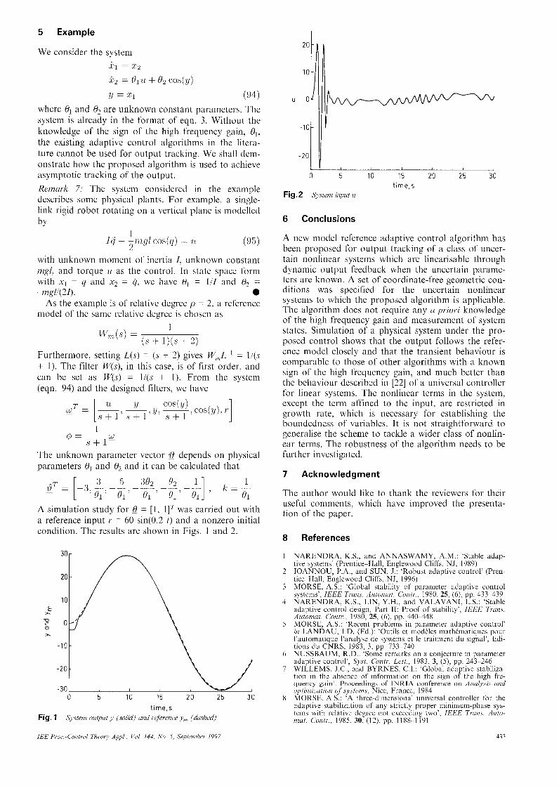
5 Example

We consider the system 2 1 = 2 z

rcz = 81.u + I92 c0”y)

y = 2 1 (94) where O1 and 0, are unknown constant parameters. The system is already in the format of eqn. 3. Without the knowledge of the sign of the high frequency gain, e,, the existing adaptive control algorithms in the litera- ture cannot be used for output tracking. We shall dem- onstrate how the proposed algorithm is used to achieve asymptotic tracking of the output. Remark 7: The system considered in the example describes some physical plants. For example, a single- link rigid robot rotating on a vertical plane is modelled by

1

rfj + lmgl 2 cms(y) = 1L (95)

with unknown moment of inertia I , unknown constant mgl, and torque U as the control. In state space form with x, = q and x2 = q, we have 8, = l/I and 13, = -mgl/(24. 0

As the example is of relative degree p = 2, a reference model of the same relative degree is chosen ab

1 Wm(s) =

( s + l)(s + 2) Furthermore, setting L(s) = (s + 2) gives W,,,L ‘ = l/(s + 1). The filter W(s), in this case, is of first order, and can be set as W(s) = l/(s + 1). From the system (eqn. 94) and the designed filters, we have

1 @ = -

S + l W

The unknown parameter vector e depends on physical parameters 19, and 19, and it can be calculated that

A simulation study for e = [ 1 , I I T was carried out with a reference input r = 60 sin(0.2 t ) and a nonzero initial condition. The results are shown in Figs. 1 and 2.

time,s Fig. 1 $y.stent output y (solid) und reference y,,, (dushed)

0 5 10 15 20 25 30 time,s

Fig. 2 Sysleni iqmt U

6 Conclusions

A new model reference adaptive control algorithm has been proposed for output tracking of a class of uncer- tain nonlinear systems which are linearisable through dynamic output feedback when the uncertain parame- ters are known. A set of coordinate-free geometric con- ditions was specified for the uncertain nonlinear systems to which the proposed algorithm is applicable. The algorithm does not require any U priori knowledge of the high frequency gain and measurement of system states. Simulation of a physical system under the pro- posed control shows that the output follows the refer- ence model closely and that the transient behaviour is comparable to those of other algorithms with a known sign of the high frequency gain, and much better than the behaviour described in [22] of a universal controller for linear systems. The nonlinear terms in the system, except the term affined to the input, are restricted in growth rate, which is necessary for establishing the boundedness of variables. It is not straightforward to generalise the scheme to tackle a wider class of nonlin- ear terms. The robustness of the algorithm needs to be further investigated.

7 Acknowledgment

The author would like to thank the reviewers for their useful comments, which have improved the presenta- tion of the paper.

References

NARENDRA, K.S., and ANNASWAMY, A.M.: ‘Stable adap- tive systems’ (Prentice-Hall, Englewood Cliffs, NJ, 1989) IOANNOU, P.A., and SUN, J.: ‘Robust adaptive control’ (Pren- lice-Hall, Englcwood Cliffs, NJ, 1996)

‘Global stability of parameter adaptive control Truns. Automat. Contr., 1980, 25, (6) , pp. 433439

NARENDRA, K.S., LIN, Y.H., and VALAVANI. L.S.: ‘Stable adaptive control design, Part 11: Proof of stability’, IEEE Tuuns. Autonzut Contr., 1980, 25, (6), pp. 440448 MORSE, A.S.: ‘Recent problems in parameter adaptive control’ in LANDAU, 1.D. (Ed.): ‘Outils et modeles mathkmatiques pour l’automatique l’analyse de systems et le traitment du signal’, Edi- tions du CNRS, 1983, 3, pp. 733-740 NUSSBAUM, R.D.: ‘Some rcmarks on a conjecture in parameter adaptive control’, Sy.rt. C‘ontr. Letl., 1983, 3, ( 5 ) , pp. 243-246 WILLEMS, J.C., and BYRNES, C.I.: ‘Global adaptive stabiliza- tion in the absence of information on the sign of the high fre- quency gain’. Proceedings of INRlA conference on Analysis ond optimizution of systems, Nice, France, 1984 MORSE, A.S.: ‘A three-dimensional universal controller for the adaptive stabilization of any strictly proper minimum-phase sys- tems with relative degree not exceeding two’, IEEE Trans. Auto- mat. Co/ztr., 1985, 30, (12), pp. 1188-1191

433 IEE Proc.-Control Theosy Appl., Vol. 144, No 5, Seplemhcr 1997

9 MUDGETT, D.R., and MORSE, M.S.: ‘Adaptive stabilization of linear systems with unknown high frequency gains’, IEEE Trans. Automat. Contr., 1985, 30, (6) , pp. 549-554

10 ISIDORI. A.: ‘Nonlinear control systems’ (Springer-Verlag, Ber- lin, 1989, 2nd edn.)

11 SASTRY, S.S., and ISIDORI, A.: ‘Adaptive control of Iineariza- ble systems’, IEEE Trans. Automat. Contr., 1989, 34, ( l l ) , pp. 1 123-1 131

I2 KANELLAKOPOULOS, I., KOKOTOVIC, P.V., and MORSE, A.S.: ‘Systematic design of adaptive controllers for feedback linearizable systems’, IEEE Trans. Automat. Contr., 1991, 36, ( I I ) , pp. 1241-1253

13 MARINO, R., and TOMEI, P.: ‘Dynamic output feedback line- arization and global stabilization’, Syst. Contr. Lett., 1991, 17, (2) , pp. 115-121

14 MARINO, R., and TOMEI, P.: ‘Global adaptive output feed- back control of nonlinear systems, Part I: Linear parameteriza- tion’, IEEE Trans. Automat. Conti., 1993, 38, (I) , pp. 17-32

434

15 KRSTIC, M., KANELLAKOPOULOS, I., and KOKO- TOVIC, P.V.: ‘Nonlinear and adaptive control design’ (J. Wiley & Sons, New York, 1995)

16 MARTENSSON, B.: ‘Remarks on adaptive stabilization of first- order adaptive systems’, Syst. Contr. Lett., 1990, 14, ( I ) , pp. 1-7

17 LOZANO, R., and BROGLTATO, B.: ‘Adaptive control of a syniple nonlinear systems without a priovi information on the plant parameters’, IEEE Trans. Automat. Contr., 1992, 37, ( l ) , nn 30-37 rr - - -

18 BRICKELL, F.R., and CLARK, R.S.: ‘Differential manifolds’

19 BOOTHBY, W.M.: ‘An introduction to differential manifolds (Van Nostrand Reinhold, London, 1970)

and Riemanian geometry’ (Academic Press, New York, 1979) 20 MARINO. R., and TOMEI, P.: ‘Nonlinear control design: geo-

metric, adaptive, and robust’ (Prentice-Hall, London, 1995) 21 SILVERMAN, L.M.: ‘Inversion of multivariable linear systems’,

IEEE Trans. Automat. Contr., 1969, 14, pp. 270-276 22 FU, M., and BARMISH, B.R.: ‘Adaptive stabilization of linear

systems via switching control’, IEEE Trans Automat. Contv., 1986, 31, (12), pp. 1097-1103

IEE Pvoc.-Control Theory A p p l , Vol. 144, No 5, Septemher 1997