Model Selection and Estimation ofMulti-Compartment Models in Diffusion MRI

with a Rician Noise Model

Xinghua Zhu1, Yaniv Gur2, Wenping Wang1, P. Thomas Fletcher2

1 The University of Hong Kong, Department of Computer Science, Hong Kong2 University of Utah, School of Computing, Salt Lake City, UT 84112, USA

Abstract. Multi-compartment models in diffusion MRI (dMRI) are usedto describe complex white matter fiber architecture of the brain. In thispaper, we propose a novel multi-compartment estimation method basedon the ball-and-stick model, which is composed of an isotropic diffusioncompartment (“ball”) as well as one or more perfectly linear diffusioncompartments (“sticks”). To model the noise distribution intrinsic todMRI measurements, we introduce a Rician likelihood term and esti-mate the model parameters by means of an Expectation Maximization(EM) algorithm. This paper also addresses the problem of selecting thenumber of fiber compartments that best fit the data, by introducing asparsity prior on the volume mixing fractions. This term provides au-tomatic model selection and enables us to discriminate different fiberpopulations. When applied to simulated data, our method provides ac-curate estimates of the fiber orientations, diffusivities, and number ofcompartments, even at low SNR, and outperforms similar methods thatrely on a Gaussian noise distribution assumption. We also apply ourmethod to in vivo brain data and show that it can successfully capturecomplex fiber structures that match the known anatomy.

1 Introduction

Diffusion Tensor Imaging (DTI) is a powerful technique that enables inferringwhite matter pathways of the brain from diffusion weighted (DW) MRI mea-surements. However, DTI can only describe one dominant diffusion directionper voxel, and therefore, cannot capture known complex fiber structures in thewhite matter in human brain. The limitation of DTI motivated the developmentof new imaging modalities that utilize higher angular resolution, as well as newmethods to extract white matter structures from such data, including sphericaldeconvolution [1], Funk-Radon transform [2], multi-compartment models [3, 4],and higher-order tensors [5–7]. In this work, we consider a particular case ofmulti-compartment models, where the diffusivities in directions perpendicularto the white matter fiber are constrained to be zero. This model is known asthe “ball-and-stick”, where the “ball” stands for the isotropic diffusion compart-ment, and each “stick” corresponds to a perfectly linear diffusion compartment(white matter fiber).

2 X. Zhu, Y. Gur, W. Wang, P.T. Fletcher

The ball-and-stick model was first proposed by Behrens et al. [8] as a con-strained version of the multi-tensor model, which comprised only one ball andone stick compartment. A Bayesian framework for the ball-and-one-stick modelestimation and tractography was also introduced in [8]. This framework waslater elaborated in [9, 4], where multiple anisotropic compartments and modelselection methods were proposed. In [9] Hosey et al. focused on the estimationof two-fiber models in a probabilistic manner under Rician noise assumption.They addressed the model selection problem by analyzing the probability den-sity function (PDF) of the Bayes Factor of the one- and two- stick models.On the other hand, the method proposed in [4] did not limit the number offiber compartments, and the estimation was done under Gaussian noise assump-tion. They adopted the automatic relevance determination (ARD) algorithmfor model selection. However, the model selection methods in [9, 4] did not dis-tinguish two-fiber models from more complicated ones, and no comprehensiveevaluation of these methods was reported. More recently, Schultz et al. [11] pro-posed a spherical deconvolution operation to estimate the fiber orientations andvolume fractions, which were refined by fitting a ball-and-stick model to the DWmeasurements. The number of fibers was selected at the spherical deconvolutionlevel by directly thresholding the associated volume fractions. Similar to [4], thisscheme did not account for the Rician noise in the DW measurements. Estima-tion of the more general two-tensor model, under Rician noise assumption, waspresented in [10].

In this paper, the parameters of the ball-and-stick model are estimated bymaximizing the log-likelihood function based on the Rician distribution. Themaximization problem is solved using an EM algorithm, where the DW mea-surements with complex Gaussian noise represent the complete data. In addi-tion, in order to find the number of compartments that best fit the data, we usea sparsity prior on the estimated volume fractions. The sparsity prior pushes tozero small volume fractions, and enables elimination of redundant terms that donot represent white matter fibers. In contrast to [9, 10], here we do not restrictour model to two stick compartments, and enable modeling of white matterstructures in brain regions that contain up to three fiber populations. The re-sults of the proposed model selection scheme provides a clear distinction betweenisotropic diffusion, and one, two, or three fiber populations.

The main contributions of this paper can be summarized as follows: 1) Wesolve the ball-and-stick estimation problem with multiple sticks, under the as-sumption of Rician noise distribution in the DW measurements. We use a Ricianlog-likelihood function which is maximized by a robust EM algorithm. 2) We as-sess the accuracy of our algorithm on simulated data at different b-values andlow SNRs, and show that it introduces less bias in the model parameters com-pared to similar algorithms that rely on a Gaussian noise assumption. 3) Weintroduce an automatic model selection scheme, which is an integral part of ourEM algorithm. This is done by introducing a sparsity prior on the volume frac-tions. 4) We evaluate the performance of the algorithm on in vivo brain data

Diffusion MRI Model Selection and Estimation with a Rician Noise Model 3

with deterministic tractography and show its ability to reproduce complex fiberstructures matching the known anatomy.

2 Rician Likelihood and Expectation Maximization

In this paper, a parametric partial volume model is used to describe the localdiffusion profile. The model we use is known as the “ball-and-sticks”, which iscomposed of a mixture of an isotropic diffusion compartment (“ball”), and multi-ple directional anisotropic diffusion compartments (“sticks”). The “sticks” corre-spond to white matter fibers, and are represented by means of the unnormalizedWatson distribution. That is, given a set of N diffusion weighted measurements,{νi}Ni=1, for each measurement in a gradient direction gi, we have

νi = S0

w0 exp(−bκ0) +

M∑j=1

wj exp(−bκj(gTi uj)

2)

, (1)

where M is the number of anisotropic compartments, S0 is the non-diffusion-weighted signal, and b represents the constant b-value. The model parameters arethe white matter fiber orientations, u1, . . . ,uM , diffusion coefficients, κ0, . . . , κM ,and volume fractions, w0, . . . , wM , where

∑Mj=0 wj = 1, wj ≥ 0.

In the rest of this paper, we will denote the set of model parameters by Θ ={u1, . . . ,uM ;w0, . . . , wM ;κ0, . . . , κM}. Also, we will use the notation νi0(Θ) =S0 ·w0 exp(−bκ0) to represent the “ball” compartment in the i-th sampled direc-tion, and νij(Θ) = S0 · wj exp(−bκj(gT

i uj)2) for the j-th “stick” compartment

in the i-th sampled direction. Using these notations, the expression for a “clean”signal in measurement direction gi is given by the sum of the compartmentsignals, νi(Θ) =

∑Mj=0 νij(Θ).

2.1 Maximum Rician Likelihood

The MR signal in the complex domain is affected by Gaussian noise. However, theDW measurements are given as the magnitude of the complex MR signal, and,therefore, the noise distribution model becomes Rician. Thus, for a measuredDW signal in the i-th gradient direction, Si, we have Si ∼ Ric(νi(Θ), σ), givenby the PDF

p(Si|Θ) =Si

σ2exp

(−S

2i + νi(Θ)2

2σ2

)I0

(Siνi(Θ)

σ2

). (2)

We will use the notation S for the set of observed DW signals, i.e., S ={Si, i = 1, . . . , N}. Assuming independent measurements in different gradientdirections, the joint PDF for the signal S in each image voxel is given by p(S|Θ) =∏N

i=1 p(Si|Θ). We estimate the parameters Θ by maximization of the likelihoodl(Θ|S) = log p(S|Θ), which is given by

l(Θ|S) = −2N log(σ) +

N∑i=1

log(Si)−S2i + νi(Θ)2

2σ2+ log I0

(Siνi(Θ)

σ2

). (3)

4 X. Zhu, Y. Gur, W. Wang, P.T. Fletcher

2.2 Expectation Maximization Algorithm

One may apply a gradient ascent method to maximize the log-likelihood function.However, when directly maximizing l(Θ|S), the optimization parameters arevariables of the modified Bessel function I0. On the other hand, the proposedEM algorithm does not involve the computation of I0 and its derivatives withrespect to the optimization parameters. Therefore, maximizing the Q-functionin the E-step is more stable numerically, and more tractable in terms of theanalytical computations involved. Indeed, we have found that the proposed EMalgorithm provides more accurate estimates of the model parameters.

Let us now consider a mixture model of one “ball” compartment and Mdifferent “stick” compartments. In the complex domain, the signal generatedby the jth compartment in the ith sampled direction is corrupted by complexGaussian noise, such that

Yij = νij(Θ) + ε, ε ∼ CN(

0,2σ2

M + 1

), (4)

where CN denotes the circularly-symmetric complex normal distribution. There-fore, the PDF and log-likelihood of the complex signal, Yij , given Θ are

p(Yij |Θ) =1

2πσ2/(M + 1)exp

(−‖Yij − νij(Θ)‖2

2σ2/(M + 1)

), (5)

l(Θ|{Yij}) =

N∑i=1

M∑j=0

− log(2πσ2/(M + 1))− ‖Yij − νij(Θ)‖2

2σ2/(M + 1). (6)

Note that the complex signal, Yij , represent the complete data in our EMalgorithm, whereas the observed incomplete data is the magnitude of a mixture

of complex signals, that is Si =∥∥∥∑M

j=0 Yij

∥∥∥, where Si ∼ Ric(νi(Θ), σ2

)[12].

The E-step is derived by calculating the expected value of the log-likelihoodwith respect to the complete data Y = {Yij , i = 1, . . . , N, j = 0, . . . ,M}:

Q(Θ|Θ(k)) = E[l(Θ|Y)|S, Θ(k)

]=

∫l(Θ|Y)p(Y|S, Θ(k))dY. (7)

Following some extensive derivations, which are too lengthy to be includedin this paper, we arrive at the final expression for the Q-function:

Q(Θ|Θ(k)) =∑i,j

2νij(Θ)

[Si

M + 1A

(Siν

(k)i

σ2

)− ν

(k)i

M + 1+ ν

(k)ij

]− νij(Θ)2,

where A(x) = I1(x)/I0(x), ν(k)i = νi(Θ

(k)), ν(k)ij = νij(Θ

(k)).In the M-step, the model parameters Θ are updated to maximize Q via

gradient ascent. The partial derivative of Q with respect to θ ∈ Θ is given by

dQ

dθ= 2

∑i,j

[Si

M + 1A

(Siν

(k)i

σ2

)− ν

(k)i

M + 1+ ν

(k)ij − νij(Θ)

]dνijdθ

. (8)

Diffusion MRI Model Selection and Estimation with a Rician Noise Model 5

The derivatives dνij/duj are computed in the tangent space of the real pro-jective space, RP2, i.e., the space of bi-directional unit vectors, due to the an-tipodal symmetry of diffusion. We write the stick components νij in terms of thegeodesic distance on RP2, that is, cos d(gi,uj) = gT

i uj . This leads to

dνij(Θ)

duj= −wjS0 exp(−bκj(cos d(gi,uj))

2)bκj sin 2d(gi,uj)

d(gi,uj)Loguj

(gi)

The derivatives dνij/dwj and dνij/dκj are straightforward to compute andare not included here. These derivatives, combined with the expression in (8),define the update step in the gradient ascent in the M-step.

3 Sparsity Prior On Compartment Fractions

When fitting to a noisy DW signal with unknown number of fiber compart-ments, an increase in the number of sticks will generally improve the modelfit. However, increasing the number of sticks beyond the true number of fibercompartments will overfit to the imaging noise. In real applications, we favorrepresentation of a diffusion profile with as few compartments as possible. Interms of the parameters, this means we favor weighting fractions that concen-trate on a minimal number of necessary compartments, rather than distributeequally upon all compartments. Therefore, we introduce a sparsity prior for thecompartment fractions.

The lp-norm with p ≤ 1 is universally used as a sparsity (or concentration)measure, where the most common choice being the l1-norm. However, the l1-norm of the volume fractions ‖(w0, . . . , wM )‖1 =

∑Mj=0 wj is constrained to be 1

in our case and cannot reflect sparsity level. Alternatively, we use the l0.5-normas the sparsity measure. That is,

C(w0, w1, . . . , wM ) =

M∑j=0

w0.5j

2

, (9)

where C gets its maximal value when all the fractions are equal, and its minimalvalue when one fraction equals to 1 and the rest equal to zero.

This term penalizes the number of compartments such that when a volumefraction, wj , tends to zero during the optimization process, the derivative dC/dwj

tends to negative infinity, which results in pushing wj faster toward zero. In thatcase, the value of wj cannot increase anymore, the associated stick compartmentwill no longer correspond to a white matter fiber, and will be eliminated from theoptimization process. We treat the sparsity penalty defined by (9) as a negativelog prior on volume fractions, which results in an amended Q function

Q̂(Θ|Θ(k)) = Q(Θ|Θ(k))− λC · C(w0, . . . , wM ), (10)

where λC is a tunable coupling factor for the sparsity constraint. Thus, in themaximization step in the EM algorithm, the derivative of C is included in thegradient ascent update of the volume fractions.

6 X. Zhu, Y. Gur, W. Wang, P.T. Fletcher

4 Implementation Details

4.1 Initialization and Model Selection

In the proposed algorithm, the number of stick compartments is automaticallyselected using the sparsity constraint.

At the beginning of the estimation, the number of stick compartments isset to 3. A 2nd-order tensor is fit to the DW signal and its eigenvectors andeigenvalues are used to initialize the stick directions and diffusivity, respectively.Initial volume fractions are set to 0.25 equally for all stick and ball compartments.

During estimation, compartments with fractions driven to zero by the spar-sity constraint are instantly removed from the model. In cases where small frac-tions of redundant compartments remain in the estimation results when the EMalgorithm converges, a set of predefined fraction thresholds, W1, W2, and W3,are applied to remove them. Given K stick compartments, those with fractionswj < WK would be removed from the estimated model. If one or more compart-ments are removed by thresholding, the EM is continued with the reduced modeluntil convergence again. Otherwise, the compartment number is determined. Wethen set λC = 0 and let the EM converge again, in order to eliminate the biasintroduced by the sparsity constraint.

In our experiments, a universal set of fraction thresholds, W1 = 0.15, W2 =0.1, and W3 = 0.05, are used in all scenarios. These values are empiricallyselected from repetitive experiments and found to provide plausible results insynthetic data with various settings. The coupling factor, λC , can be set withrespect to different b-value and SNR scenarios. In particular, we tune the valueof λC to perform optimally on simulated training data (independent from thetesting data in the results section) with the given b-value and SNR.

4.2 Assumptions on Diffusivity

It is known that indeterminacy prevents simultaneous estimation of diffusivitiesand volume fractions when the DW measurements are available for a single b-value only [13]. As we use the volume fractions for automatic model selection,constraining assumptions are made on diffusivity values to resolve parameterindeterminacy.

We first assume that the ball diffusivity is known and constant in a dataset,and let the algorithm determine the optimal fraction of the ball compartmentfor a given diffusivity. In practice, even though the ball diffusivity and volumefraction are in-determinant for a single voxel, we can estimate a common balldiffusivity from a collection of voxels. We discuss this process in the next section.

Secondly, we assume that all stick compartments in one voxel have the samediffusivity. This assumption helps to distinguish stick compartments from theball. A stick compartment degenerates into a ball compartment when its diffu-sivity approaches zero. With this constraint, when a stick compartment is redun-dant, the EM algorithm inclines to decrease its fraction instead of its diffusivity,so it prevents the emergence of an additional isotropic compartment.

Diffusion MRI Model Selection and Estimation with a Rician Noise Model 7

4.3 Estimating Ball Diffusivity

As the ball diffusivity is assumed to be known in the proposed estimation al-gorithm, its value needs to be determined from the given data. Yet, when theball diffusivity and fraction are both unknown, indeterminacy between the twoparameters prevents reliable estimation of either of them. To solve this problem,based on the assumption that the true ball diffusivity is constant in the dataset,we propose the following procedure to estimate its value. We first select a num-ber of voxels with a single-fiber configuration. Then, we fit a ball-and-one-stickmodel to these voxels by alternating between estimating the diffusivities and thevolume fractions, with the other fixed. After each iteration, the median of thediffusivities / fractions among all selected voxels are used to initiate the nextround of estimation. After a few iterations, the median values would convergeand the median ball diffusivity at convergence is taken as the ball diffusivity forthe given dataset.

5 Results

5.1 Simulated Data

First, we tested the performance of the proposed method on simulated data.The clean DW measurements were synthesized using the ball-and-stick modelwith 64 gradient directions. In the simulation, all ball and stick compartmentshad the same volume fraction, 1/(M + 1), where M was the number of stickcompartments simulated. The stick and ball diffusivities were derived to closelysimulate real white matter and were set as 1.54× 10−3 and 8.83× 10−4, respec-tively. The simulated DW signal was corrupted by Rician noise using a standardprocedure where a complex Gaussian noise was added to the signal, and we tookthe modulus of the noisy signal in the complex domain.

The proposed method was evaluated at b-values of 2000 and 3000, and base-line SNRs of 15 and 20. For each scenario 100 noisy signal instances were gen-erated to gather statistical evaluation of the estimation performance.

For each pair of b-value and SNR, we randomly picked 50 samples from thesingle-fiber signals and applied the method described in Section 4.3 to recoverthe ball diffusivity.

Parameter estimation accuracy. We assessed the accuracy of our algorithmin various cases that differed by the separation angle and the number of simu-lated compartments. We compared our results with the ball-and-stick estimationscheme proposed by Schultz et al. [11]. Also, to compare the reconstruction be-havior between Rician and Gaussian noise models, we implemented a variant ofour method where the Rician likelihood was replaced with the Gaussian likeli-hood. In this experiment, we fixed the number of stick compartments in boththe algorithm of [11] and our algorithm (and, thus, turned off the sparsity priorby setting λC = 0).

8 X. Zhu, Y. Gur, W. Wang, P.T. Fletcher

b-value SNR = 15 SNR = 20

2000

0

1

2

3

4

5

6

7

8

9

Angula

r E

rror

(degre

es)

M = 1

α = N\A

M = 2

α = 45°

M = 2

α = 50°

M = 2

α = 60°

M = 2

α = 90°

M = 3

α = 90°

Rician ML

Gaussian ML

Schultz et al’s algorithm

0

1

2

3

4

5

6

7

8

9

Angula

r E

rror

(degre

es)

M = 1

α = N\A

M = 2

α = 45°

M = 2

α = 50°

M = 2

α = 60°

M = 2

α = 90°

M = 3

α = 90°

Rician ML

Gaussian ML

Schultz et al’s algorithm

3000

0

1

2

3

4

5

6

Angula

r E

rror

(degre

es)

M = 1

α = N\A

M = 2

α = 45°

M = 2

α = 50°

M = 2

α = 60°

M = 2

α = 90°

M = 3

α = 90°

Rician ML

Gaussian ML

Schultz et al’s algorithm

0

1

2

3

4

5

6

Angula

r E

rror

(degre

es)

M = 1

α = N\A

M = 2

α = 45°

M = 2

α = 50°

M = 2

α = 60°

M = 2

α = 90°

M = 3

α = 90°

Rician ML

Gaussian ML

Schultz et al’s algorithm

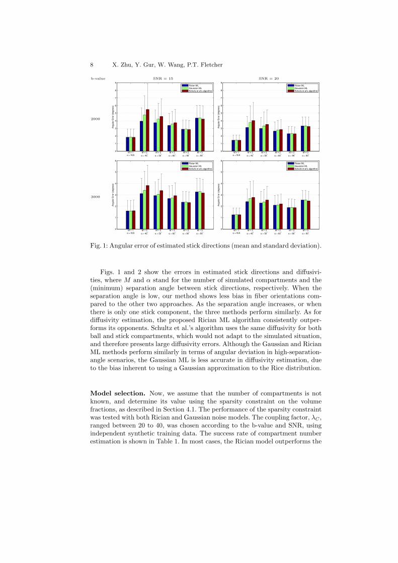
Fig. 1: Angular error of estimated stick directions (mean and standard deviation).

Figs. 1 and 2 show the errors in estimated stick directions and diffusivi-ties, where M and α stand for the number of simulated compartments and the(minimum) separation angle between stick directions, respectively. When theseparation angle is low, our method shows less bias in fiber orientations com-pared to the other two approaches. As the separation angle increases, or whenthere is only one stick component, the three methods perform similarly. As fordiffusivity estimation, the proposed Rician ML algorithm consistently outper-forms its opponents. Schultz et al.’s algorithm uses the same diffusivity for bothball and stick compartments, which would not adapt to the simulated situation,and therefore presents large diffusivity errors. Although the Gaussian and RicianML methods perform similarly in terms of angular deviation in high-separation-angle scenarios, the Gaussian ML is less accurate in diffusivity estimation, dueto the bias inherent to using a Gaussian approximation to the Rice distribution.

Model selection. Now, we assume that the number of compartments is notknown, and determine its value using the sparsity constraint on the volumefractions, as described in Section 4.1. The performance of the sparsity constraintwas tested with both Rician and Gaussian noise models. The coupling factor, λC ,ranged between 20 to 40, was chosen according to the b-value and SNR, usingindependent synthetic training data. The success rate of compartment numberestimation is shown in Table 1. In most cases, the Rician model outperforms the

Diffusion MRI Model Selection and Estimation with a Rician Noise Model 9

b-value SNR = 15 SNR = 20

2000

0

1

2

3

4

5

6

7

8

Diffu

siv

ity E

rror

(× 1

0−

4 m

m2/s

)

M = 1

α = N\A

M = 2

α = 45°

M = 2

α = 50°

M = 2

α = 60°

M = 2

α = 90°

M = 3

α = 90°

Rician ML

Gaussian ML

Schultz et al’s algorithm

0

1

2

3

4

5

6

7

8

Diffu

siv

ity E

rror

(× 1

0−

4 m

m2/s

)

M = 1

α = N\A

M = 2

α = 45°

M = 2

α = 50°

M = 2

α = 60°

M = 2

α = 90°

M = 3

α = 90°

Rician ML

Gaussian ML

Schultz et al’s algorithm

3000

0

1

2

3

4

5

6

7

8

Diffu

siv

ity E

rror

(× 1

0−

4 m

m2/s

)

M = 1

α = N\A

M = 2

α = 45°

M = 2

α = 50°

M = 2

α = 60°

M = 2

α = 90°

M = 3

α = 90°

Rician ML

Gaussian ML

Schultz et al’s algorithm

0

1

2

3

4

5

6

7

8

Diffu

siv

ity E

rror

(× 1

0−

4 m

m2/s

)

M = 1

α = N\A

M = 2

α = 45°

M = 2

α = 50°

M = 2

α = 60°

M = 2

α = 90°

M = 3

α = 90°

Rician ML

Gaussian ML

Schultz et al’s algorithm

Fig. 2: Root mean square error of the estimated diffusivities.

Gaussian one, especially at low SNRs. The only cases where the Gaussian MLperforms better are at SNR=20 and a separation angle of 45◦.

In addition, we compared the proposed model selection method with theAkaike Information Criteria (AIC). As shown in Table 1, AIC produces plausibleresults only for isotropic, or single fiber configurations. It is found that AICis very conservative in choosing the optimal number of parameters, such thatit always underestimates the number of compartments for complex diffusionstructures. We have also found that the similar Bayesian Information Criteria(BIC) is even more conservative than the AIC.

5.2 In Vivo Brain Data

The human brain data was acquired on a 3T Siemens Allegra Tim Trio scannerusing a b-value of 2000 s/mm2. The scan was composed of 10 B0 volumes and60 diffusion weighted volumes of matrix size 128 × 128 × 70, and voxel size of2×2×2 mm3. The volumes were registered to a T1 template with a voxel size of1 mm3, and corrected for motion, eddy current, and EPI distortions. The Riciannoise parameter σ was estimated from background voxels as σ̂ =

√var(S)/2. To

determine the ball diffusivity in the brain data, 50 voxels were selected in thecorpus callosum region, where the number of sticks was known to be 1. Followingthe procedure in Section 4.3, the ball diffusivity was estimated as 8.8294×10−4.

We selected a 41×41×41 region of the brain data for experimental evaluation.In the selected region, the SNR was estimated to be approximately 25. We chose

10 X. Zhu, Y. Gur, W. Wang, P.T. Fletcher

Compartment no. 0 1 2 3Separation angle - - 45◦ 50◦ 60◦ 90◦ 90◦

Rician ML w/Sparsity Prior

b-value = 2000SNR=15 98 100 75 95 100 100 100SNR=20 100 100 83 99 100 100 100

b-value = 3000SNR=15 100 100 72 96 98 100 100SNR=20 100 100 71 98 100 100 100

Gaussian ML w/Sparsity Prior

b-value = 2000SNR=15 100 84 73 74 73 69 100SNR=20 100 96 90 91 90 86 100

b-value = 3000SNR=15 100 85 71 77 77 74 100SNR=20 100 96 89 91 93 93 100

Rician ML w/ AICb-value = 2000

SNR=15 100 100 0 0 0 29 0SNR=20 100 100 0 0 0 99 0

b-value = 3000SNR=15 100 100 0 0 0 83 0SNR=20 100 100 0 0 8 100 15

Table 1: Accuracy of number of compartments determination (in percentage).

the sparsity prior coupling factor λC = 75 using a few synthesized trainingsamples of the same b-value and SNR.

Figure 3(a) and (b) show the parameter estimation and automatic modelselection results with the proposed method. It is easy to identify the corpus cal-losum where the one-stick model was selected, with a clear boundary against theisotropic background. Meanwhile, the 3-stick model was selected in the crossingregion of the corpus callosum, cortical spinal and SLF. The pattern of the num-ber of sticks is highly consistent with known anatomy of the white matter in thebrain. Some erroneous model selection results can be spotted in the CSF, andat the boundary between the CSF and the white matter tracts, where 3 sticksare attributed. This is likely to result from an underestimated ball diffusivity.

As a comparison, we used the voxel classification method in Camino [14]to select the optimal order of spherical harmonics for the diffusion data, whichapplied Alexander et al.’s algorithm using an F-test [15]. In this method, threeclasses are detected with corresponding spherical harmonics orders 0, 2, and 4,which stand for isotropic diffusion, single directional diffusion tensor, and com-plex diffusion structures consisting of two or more fiber orientations, respectively.We set the background signal threshold as 100 and the thresholds for separatingthe three classes as 1× 10−20, 1× 10−6 and 1× 10−6. As shown in Figure 3(d),the output of the F-test is noisy and does not match the anatomy well, especiallyin the crossing region of the three tracts.

We used the deterministic tractography tool in Camino to perform fibertracking from our reconstruction results. The fibers were seeded in every voxelwhere our method detected one or more stick compartments. Following the trac-tography process, ROIs were used separately to select fiber bundles in the corpuscallosum, cortical spinal and SLF, respectively, as shown in Figure 3(e) - (g). Forthe corpus callosum, tractography from the reconstructed ball-and-stick modelreproduced the U-shaped callosal radiation and also the lateral transcallosal

Diffusion MRI Model Selection and Estimation with a Rician Noise Model 11

(a)

0

1

2

3

(b)

0

1

(c)

0

2

4

(d)

(e) (f) (g)

Fig. 3: Automatic model selection and reconstruction results on in vivo braindata. (a) Location of the selected section and the stick orientations (weightedby associated fractions) reconstructed with the proposed method; (b) stick com-partment numbers estimated with the proposed method; (c) stick compartmentnumbers estimated with AIC; (d) the order of spherical harmonics selected by F-test; (e) - (g) tractography results from the reconstructed ball-and-stick modelsfor (e) corpus callosum, (f) cortical spinal, and (g) SLF (sagittal slice).

fibers. In addition, the tractography yielded the cortical spinal going from bot-tom to top, as well as the SLF bundle in the front-back direction. All the threetracts crossed at the center region of the depicted section.

6 Conclusions

In this paper, we proposed a novel scheme for estimating parameters in a multi-compartment model that is composed of an isotropic “ball” compartment, andmultiple perfectly linear “stick” compartments, under Rician noise assumption.Our scheme combines a robust Rician EM algorithm, and a sparsity prior on thevolume mixing fractions to automatically select the number of compartments.Using simulated data, we showed that our formulation reduces bias in the estima-tion of fiber orientations, diffusivities, and number of compartments, comparedto alternative schemes that rely on a Gaussian noise assumption. Furthermore,we applied the proposed algorithm to in vivo brain data and show that ourmethod provides a clear distinction between different fiber populations, and isable to reconstruct fiber pathways that match known white matter structuressuch as the transcallosal fibers.

Acknowledgements. This project was supported in part by grants R01 MH084795,5P41RR012553-14, and 8P41GM103545-14 from the National Institutes of Health.

12 X. Zhu, Y. Gur, W. Wang, P.T. Fletcher

References

1. Tournier, Calamante, F., Gadian, D.G., Connelly, A.: Direct estimation of thefiber orientation density function from diffusion-weighted MRI data using sphericaldeconvolution. NeuroImage 23(3) (November 2004) 1176–1185

2. Descoteaux, M., Angelino, E., Fitzgibbons, S., Deriche, R.: Regularized, fast, androbust analytical Q-ball imaging. Magn. Res. Med. 58(3) (2007) 497–510

3. Tuch, D.S., Reese, T.G., Wiegell, M.R., Wedeen, V.J.: Diffusion MRI of ComplexNeural Architecture. Neuron 40(5) (December 2003) 885–895

4. Behrens, T.E., Berg, H.J., Jbabdi, S., Rushworth, M.F., Woolrich, M.W.: Proba-bilistic diffusion tractography with multiple fibre orientations: What can we gain?NeuroImage 34(1) (January 2007) 144–155

5. Liu, C., Bammer, R., Acar, B., Moseley, M.E.: Characterizing non-gaussian dif-fusion by using generalized diffusion tensors. Magn. Reson. Med. 51(5) (2004)924–937

6. Weldeselassie, Y., Barmpoutis, A., Atkins, M.S.: Symmetric positive-definite carte-sian tensor orientation distribution functions (CT-ODF). In Jiang, T., Navab, N.,Pluim, J., Viergever, M., eds.: MICCAI’10. Volume 6361 of LNCS., Springer, Hei-delberg (2010) 582–589

7. Jiao, F., Gur, Y., Johnson, C.R., Joshi, S.: Detection of crossing white matterfibers with high-order tensors and rank-k decompositions. In: IPMI’11. Volume6801 of LNCS., Berlin, Heidelberg, Springer-Verlag (2011) 538–549

8. Behrens, T.E.J., Woolrich, M.W., Jenkinson, M., Johansen-Berg, H., Nunes, R.G.,Clare, S., Matthews, P.M., Brady, J.M., Smith, S.M.: Characterization and propa-gation of uncertainty in diffusion-weighted MR imaging. Magn. Reson. Med. 50(5)(November 2003) 1077–1088

9. Hosey, T., Williams, G., Ansorge, R.: Inference of multiple fiber orientations in highangular resolution diffusion imaging. Magn. Reson. Med. 54(6) (2005) 1480–1489

10. Caan, M., Khedoe, H., Poot, D., den Dekker, A., Olabarriaga, S., Grimbergen, K.,van Vliet, L., Vos, F.: Estimation of diffusion properties in crossing fiber bundles.Medical Imaging, IEEE Transactions on 29(8) (aug. 2010) 1504 –1515

11. Schultz, T., Westin, C.F., Kindlmann, G.: Multi-diffusion-tensor fitting via spheri-cal deconvolution: a unifying framework. In: Proceedings of the 13th internationalconference on Medical image computing and computer-assisted intervention: PartI. MICCAI’10, Berlin, Heidelberg, Springer-Verlag (2010) 674–681

12. Marzetta, T.L.: EM algorithm for estimating the parameters of a multivariatecomplex Rician density for polarimetric SAR. In: 1995 International Conferenceon Acoustics, Speech, and Signal Processing. Volume 5., IEEE (1995) 3651–3654

13. Scherrer, B., Warfield, S.K.: Why multiple b-values are required for multi-tensormodels. Evaluation with a constrained log-Euclidean model. In: Proc. of the 7thIEEE International Symposium on Biomedical Imaging (ISBI). (2010) 1389–1392

14. Cook, P., Bai, Y., Nedjati-Gilani, S., Seunarine, K., Hall, M., Parker, G., Alexan-der, D.: Camino: Open-source diffusion-mri reconstruction and processing. In:14th Scientific Meeting of the International Society for Magnetic Resonance inMedicine. Volume 2759. (2006)

15. Alexander, D., Barker, G., Arridge, S.: Detection and modeling of non-gaussianapparent diffusion coefficient profiles in human brain data. Magnetic Resonancein Medicine 48(2) (2002) 331–340