Model validation and experimentally driven hydraulic damper model refinement

B. Titurus, N.A.J. Lieven University of Bristol, Department of Aerospace Engineering Queens Building, University Walk, Bristol, BS8 1TR, UK email: brano.titurus@bristol.ac.uk

Abstract The paper presents study of the issues related to modelling of hydraulic damper with mechanical relief valves. This structural component plays essential role in helicopter applications where it provides damping augmentation against vibration instabilities. Previous research has established baseline damper model, which is based on the concepts from hydraulic system theory. The parametric dynamic model of a damper is used along with set of validation experiments to analyse the quality of a baseline model and its potential for improvement. Concurrent use of damper response data taken from a mathematical model and an experiment enables closer inspection of the physical mechanisms previously not included in a given reference model, as well as detailed analysis related to uncertain aspects of the model. A set of experiments is performed on the two nominally identical dampers and the data originating from these experiments are compared with corresponding responses of the mathematical model of the damper.

1 Introduction

This paper presents a study of selected problems associated with model of hydraulic damper used in rotorcraft applications. A lag damper is a passive energy dissipating component whose primary role is to provide damping augmentation in lead-lag blade motion in unsteady operational regimes such as helicopter take-off, landing, sudden manoeuvres etc. Historically, this component provided an answer to early problems with the phenomenon of so called ground resonance originating from the introduction of flapping and lead-lag hinges, constituting an articulated rotor arrangement. Nowadays, standard configurations of these dampers utilise hydro-mechanic principles to achieve required operational characteristics. Hydraulic dampers are designed to provide prescribed operational behaviour, where the general expectation is that the damper would produce high motion resisting forces for relatively small blade lag velocities to ensure stability. Further, to avoid excessive load transfer to blades and rotor hub, the damper forces have to be limited to structurally acceptable limits. This is usually achieved by mechanical means by use of secondary by-pass fluid flow paths in the damper equipped with relief valves activated when the threshold forces are reached. This process effectively represents a hydro-mechanic approximation of friction damper capabilities, whose practical implementations represented early embodiments of helicopter lag dampers. There is ongoing interest to generate reliable models of these devices. Parametric models are frequently used due to their relatively versatile application in complex simulation scenarios and in further analytical and design studies. Original interest in this subject came from the mechanical engineering community, particularly for use in car and transportation industries. Early reference of this work is presented in [1]. More recent references from mechanical engineering field dealing with parametric modelling of hydraulic dampers and shock absorbers are [2] and [3]. Later, the application of discrete damping devices in vibration suppression, earthquake and general critical event protection induced similar interest in civil engineering with applications on bridge structures and high-rise buildings particularly. Recent studies of nonlinear viscous dampers are provided in [4] and [5]. Finally, there has been recent interest in the

rotorcraft industry to introduce models of sufficient refinement to improve the quality of predictions provided by integrated aero-elastic simulation tools. Work presented in this paper is based on previous analytical studies investigated in [6]. Moreover, similar work investigating a hydraulic lag damper was also presented in [7]. Importance of lag damper modelling in the full rotor context stems from the fact that in certain design configurations it represents a significant force contributor to the overall blade loading system. Therefore, its satisfactory modelling is of great importance for design performance studies. Previous work on this damper has been presented in [6] and is further extended here. Firstly, the model is experimentally tested by a standard test procedure originally specified for damper qualification purposes. Resulting data provide a basis for comparison with equivalent data generated by the model. The second element of the work is model refinement based on observations resulting from previous comparative baseline study. The goal of this paper is validation of the reference model and analysis of its refinement potential along with evaluation of consequences and trade-off associated with increasing detail of damper modelling. Based on previous comments, the paper is divided into an analytical and an experimental part. Within Section 2 basic modelling principles are briefly reviewed such that the baseline model from [6] can be introduced in Section 2.2. This model is further extended or refined in Section 2.3, while the reasons and detailed arguments towards this step are introduced in experimental part of the paper. A description of the test conditions is given in Section 3.1. Results for both baseline and extended damper model are provided in Section 3.2. An analysis of observed results is given in Section 3.3. Finally, as the component investigated in this study represents a functional rotorcraft industrial-scale device, analysis in this paper restricts only to qualitative analysis of observed and simulated results. Thus, all presented case-specific details are provided in dimensionless and consistently scaled form allowing evaluation of trends and internal or relative data comparisons.

2 Model of helicopter lag damper

2.1 Basic modelling concepts

A few fundamental concepts can be used in construction of a lag damper model. Out of multiple physical features and regimes only a few are selected for baseline and extended lag damper modelling. To restrict the initial complexity of the model to be within realistic bounds, a number of features are not considered in this paper. A brief discussion about these elements will be presented in subsequent sections. Hydraulic dampers can be viewed as unsteady high-pressure hydraulic circuits with internal fluid circulation. Performance of these systems is affected by compressibility effects. They introduce into system both hysteresis and uncertainty. An isothermal tangent fluid compressibility is considered here

( ) /F p V dV d pβ =− , where V is the fluid volume and p is the homogeneous pressure of the fluid. In this paper constant fluid compressibility is assumed such that ,0 ( )F F pβ β≈ . Fluid bulk modulus is defined as ,0 ,01/F FB β= . Some other effects are included as well such as container flexibility and gas/air volume entrapped in the container. These effects represent additive volumetric modifications in the above definition of compressibility and therefore they lead to a spring-in-series arrangement of stiffness-like quantities, which in this case is the bulk modulus. A formula suggesting critical influence of these other compressibility sources can be written as follows [8]

( ) ,0

1 1 1 1 1eff

ieff i F C GB B B B Bβ ∗= = ≈ + +∑ (1)

where 1/eff effB β= is the overall effective or apparent (fluid) bulk modulus, 1/C CB β= is the bulk modulus due to container flexibility (e.g. ( / )C C CB h d E≈ for a thin-walled container with wall thickness Ch ,

internal container diameter Cd and modulus of elasticity E of container material [Merritt]) and 1/G GB β∗ ∗=

is the volumetrically proportionate bulk modulus due to entrapped gas/air, ( / )G C G GB V V B∗ ≈ , CV is total volume of fluid container, GV is volume of the gas/air entrapped in the container and 1/G GB β= is the gas/air bulk modulus, [8]. A compressible hydraulic container with a number of flow inputs and outputs provided by an arrangement of orifices flow paths can be derived from the mass conservation condition / in outm dm dt m m≡ = − . Its application for a specific fluid chamber of variable volume iV and assumption of homogeneous fluid density ρ leads to the equation of flow rate equilibrium used in hydraulic system modelling:

, , ,( ) ( )( ) ( )i eff i i i in j ij out k ikj k

V V p Q p Q pβ+ = ∆ − ∆∑ ∑ (2)

where dot over quantities above represents time derivative, ,in jQ is j-th volumetric flow rate into i-th chamber, ,out kQ is k-th volumetric flow rate out of i-th chamber and rsp∆ is the pressure difference between two interconnected chambers r and s. Two types of fluid paths considered are the orifice and its generalisation – the relief valve. Fluid paths act as flow restrictors and their properties can be abstracted by their static characteristic ( )Q q p= ∆ [8], where Q is the volumetric flow rate through the flow restricting element and p∆ is the pressure difference across the element. For an orifice, based on Bernoulli equation, the static characteristic can be written [8]

,( ) sign( ) 2 /O D O OQ p p C A p ρ∆ = ∆ ∆| | (3)

where sign( ) is the signum function, ,D OC is the orifice discharge coefficient (whose value depends on orifice type, fluid speed, etc.), OA is the orifice cross-sectional area and ρ is fluid density. This form can be further generalised for the case of relief valves [9] such that

,( ) sign( ) ( ) ( ) 2V D V V V VQ p p C x A x p ρ∆ = ∆ ∆| |/ (4)

where , , ,0( ) /(1 )D V V D V V VC x C x xγ γ= + is the variable valve discharge coefficient with , ,0D VC and γ determined experimentally, ( ) sin( )V V V VA x d xπ α= is the variable valve area freed by moving the valve’s

poppet from its seat, Vd is the valve seat diameter and α is the half-angle of the assumed poppet’s cone.

Inclusion of a mechanical moving element in the damper’s design to represent the relief valve necessitates the use of corresponding mechanical motion equations. If given valve design is assumed to be abstracted as a mass supported on a pre-compressible spring, [9], its baseline equation has the standard form

( ) ( )V V V V V V ext hydrom x b x k x F t F t+ + = ≈ (5)

where , ,V V Vm b k are the poppet mass, effective damping and stiffness of relief valve system, respectively ,

and external forces extF acting on moving element of the valve is assumed to be dominated by the hydraulic force hydroF due to pressure difference p∆ seen by the valve’s poppet. The equation of the relief valve (5) establishes a link between constituent physical components – hydraulics and mechanics. The form of representation of this force is case specific. One version suitable for a valve with a conic poppet is presented by Hayashi et al. in [9] for a valve with seat cross-section area VA as follows

, ,0( ) 1 4 /(1 ) ( / )sin(2 ) ( ).hydro V D V V V V V V V VF t A p C x x x d A p G xγ γ α= ∆ − + ∆[ ]{ }= (6)

2.2 Baseline model of the damper

Previously introduced hydraulic and mechanical modelling concepts establish the basis for construction of a baseline model of the damper. The organisation of the damper is presented in Figure 1. It represents a damper with a through-rod in a fully symmetrical arrangement. The piston head includes the main orifice

controlling damping levels for small piston excitation velocities Py , i.e. inducing sharply rising damper forces DF for small Py . The overall orientation of the damper in the rotor hub context is indicated in the figure. Functionally, the damper is complemented with external by-pass routes with one relief valve for both flow directions, induced by forced piston oscillatory motion. The valve’s functionality is implemented via a pre-compressed spring establishing a suitable symmetrical threshold value ,D TF| | for valve activation. This feature provides the capability to reduce the rate of growth of DF with increasing

Py . Functionally, therefore, the damper effectively approximates behaviour of standard friction damper.

The two working chambers of the damper are filled with standard silicon based working hydraulic fluid. To provide background pressure – as well as a reservoir for excessive or lost fluid due to temperature changes or seepage, respectively – a compensation chamber is used and it constitutes a secondary part of the damper implementation. However, this feature is not included in the current model.

Chamber 1 Chamber 2yP(t)

FD (t)

Attachment to hub

Attachment to blade

Fixed orifice

Directional relief valves

Figure 1: Basic layout of symmetric hydraulic lag damper

Based on previous functional description as well as modelling an introduction provided in section 2.1 the model of the damper consists of two main parts: hydraulic and mechanical. The mathematical model of the damper presented in this section was introduced and extensively studied by Eyres in [6].

An assumption of a symmetric arrangement allows use of a differential pressure 1 2p p p∆ = − . Its application along with the flow rate balance equation (2) for both working chambers results in the hydraulic part of the damper model, [6], being

( ),0 1

( ) 1 sign( ) ( ) ( , ) ( , ) ,P P O V V VF

d p A y p Q p p x Q p xdt V

ζβ ζ

∆ + ⎡ ⎤= − ∆ ∆ + ∆ ∆⎣ ⎦D | | | | | | | | (7)

where 2 1V Vζ= represents the relationship between the volumes of the two working chambers, ζ +∈ , OQ is the flow rate through the main piston orifice based on equation (3) and VQ is the flow rate through the relief valves if open based on equation (4). As indicated by equation (7), flow direction for both fluid passages is based on sign( )p∆ . This model assumes a single, or no valve open in any given time instant, which is a valid assumption for standard operational conditions, [6]. The openness logical operator D controls the contribution of relief valves to the flow rate balance equation such that: a) 1=D if either

CRITp P∆ >| | or ,1(2) 0Vx >| | , or b) 0=D if CRITp P∆ ≤| | and ,1(2) 0Vx =| | . CRITP is the critical pressure difference for which the pre-compression of the springs in relief valves is overcome allowing fluid flow. The mechanical part of the model is represented by a state-space representation of equation of motion of the j-th valve based on equation (5), where identity , ,/V j V jd x dt x= is complemented with

, , , , , , ,/ ( ( )) / , 1,2.V j hydro j V j V j V j V j CRIT V jd x d t F b x k x X m j= − − =∓ (8)

CRITX is the spring pre-compression establishing required critical pressure difference CRITP such that /CRIT V CRIT VP k X A= , assuming an equal setup for both relief valves.

The complete model is represented by conditional, non-autonomous, nonlinear state-space differential equations of the form ( , ; )t=x f x p , where 5

,1 ,1 ,2 ,2, , , , TV V V Vx x x x p= ∆ ∈x [ ] is the state vector and PN∈p is

a vector of physical parameters of the damper model.

2.3 Extended model of the damper

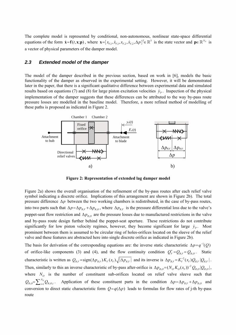
The model of the damper described in the previous section, based on work in [6], models the basic functionality of the damper as observed in the experimental setting. However, it will be demonstrated later in the paper, that there is a significant qualitative difference between experimental data and simulated results based on equations (7) and (8) for large piston excitation velocities Py . Inspection of the physical implementation of the damper suggests that these differences can be attributed to the way by-pass route pressure losses are modelled in the baseline model. Therefore, a more refined method of modelling of these paths is proposed as indicated in Figure 2.

Chamber 1 Chamber 2yP(t)

FD (t)

Attachment to hub

Attachment to blade

Fixed orifice

Directional relief valves

∆pR,V ∆pR,O

∆p

a) b)

Figure 2: Representation of extended lag damper model

Figure 2a) shows the overall organisation of the refinement of the by-pass routes after each relief valve symbol indicating a discrete orifice. Implications of this arrangement are shown in Figure 2b). The total pressure difference p∆ between the two working chambers is redistributed, in the case of by-pass routes, into two parts such that , ,R V R Op p p∆ =∆ +∆ , where ,R Vp∆ is the pressure differential loss due to the valve’s poppet-seat flow restriction and ,R Op∆ are the pressure losses due to manufactured restrictions in the valve and by-pass route design further behind the poppet-seat aperture. These restrictions do not contribute significantly for low piston velocity regimes, however, they become significant for large Py . Most prominent between them is assumed to be circular ring of holes-orifices located on the sleeve of the relief valve and these features are abstracted here into single discrete orifice as indicated in Figure 2b).

The basis for derivation of the corresponding equations are: the inverse static characteristic 1( )p q Q−∆ = of orifice-like components (3) and (4), and the flow continuity condition , ,V R V R OQ Q Q∗ = = . Static

characteristic is written as , , ,sign( ) ( )R V R V V V R VQ p K x p= ∆ ∆| | and its inverse is 2, , ,( )R V V V R V R Vp K x Q Q−∆ = | | .

Then, similarly to this an inverse characteristic of by-pass after-orifice is 2, , ,( ( ))R O O O V R O R Op N K x Q Q−∆ = | | ,

where ON is the number of constituent sub-orifices located on relief valve sleeve such that

, , ,1ON

R O R O iiQ Q

==∑ . Application of these constituent parts in the condition , ,R V R Op p p∆ =∆ +∆ and

conversion to direct static characteristic form ( )Q q p= ∆ leads to formulas for flow rates of j-th by-pass route

, , , ,

2 2 2 2 2 1/ 2, , , , , , , , , ,

( , ) sign ( ) ( ) 2 / ,

( ) 1/( ( ) ( )) 1/( )V j V j V j V j

V j V j D V j V j V j V j O D j O j O

Q p x p K x p

K x C x A x N C A

ρ∗ ∗

∗ −

∆ = ∆ ∆

= + }

| |

{ (9)

where , ,D j OC is the discharge coefficient and ,j OA is the cross-sectional area of a single valve’s sleeve orifice located on the j-th relief valve by-pass route. Equation (9) for flow rate through the j-th by-pass route due to a combination of flow restrictors according to Figure 2b) can be directly substituted into the hydraulic part of the damper model (7).

A compressible fluid with ,0 0Fβ ≠ leads to a nonzero term ,0 1( ) /(1 )FQ V pβ β ζ ζ= + ∆{ } in the flow-rate equilibrium equation (7). Flow-rate Qβ causes a hysteretic behaviour of the system. Equation (1) indicates that the overall “stiffness” of the system is determined by its “softest” component. Even a relatively low gas/air content in the total volume introduces a very low “stiffness” represented by GB , where – for instance – a 1% air content results into 100G GB B∗= . A similar observation can be indicated for CB and similar features. Therefore, ,0Fβ in equation (7) is directly substituted by overall effective

compressibility of the system as indicated by equation (1), i.e. ( )eff rr

β β=∑ , where r represents different

sources of capacitive behaviour in the system. Based on previous comments, equation (7) can be written directly in the following form

( ), , ,1

( ) 1 sign( ) ( ) ( , ) ( , ) .P P O V j V j V jeff

d p A y p Q p p x Q p xdt V

ζβ ζ

∗∆ + ⎡ ⎤= − ∆ ∆ + ∆ ∆⎣ ⎦D (10)

Finally, the previous model extension considerations have further implications on the mechanical part of the model through equations (8), where the formula (6) for hydroF has to be modified to take into account

p∆ redistribution due to an additional orifice in the by-pass flow path. The hydraulic force then has the form ,hydro V R V VF A p G= ∆ , where 2 2

, , , , ,( ( )) ( )R V O O V V j V j V V V j V jp p N K x Q Q K x Q Q− ∗ ∗ − ∗ ∗∆ =∆ − | |= | |.

3 Experimental lag damper testing and correlation studies

3.1 Test specification and experimental configuration

To evaluate fidelity and limitations of above two versions of hydraulic lag damper configurations shown in Figure 1 and Figure 2 their simulated responses will be compared with compatible data recorded in the experimental setup shown in Figure 3.

PC

yp,meas

FDHydraulic actuator Damper

yp,meas , FD

yp,command

Figure 3: Lag damper test setup

A horizontal chain-like arrangement of linear servo-hydraulic Instron actuating system provided forced excitation of damper’s piston in the form of prescribed piston displacement forms. Both, damper and

actuator are attached to the braces are further fixed to the base floor. This arrangement is further strengthened by a vertical steel bar directly connecting attachment braces. The two measured quantities in this arrangement are the actual piston displacement , ( )P measy t provided by LVDT integrated in the actuator and the force , ( )D measF t between damper and actuator pistons measured via a load cell located as indicated in Figure 3. The damper is attached to the brace and load cell attachment fixture via universal joints to minimise non-axial force transmission. A prescribed excitation signal , ( )P commandy t is provided and generated by an Instron proprietary system with a PID-based closed loop control of actuation difference

, ,P command P measerr y y= − .

Measured , ( )P measy t is further post-processed to generate , ( )P measy t utilising 4-th order polynomial Savitzky-Golay filter as implemented in Matlab, [10]. The damper force generated by the models provided in section 2 is approximated as follows

,

sign( )D P P P P f P

D meas D fix P D

F A p m y y F A pF F m y F

= ∆ + − ≈ ∆

= + ≈

| | (11)

where contributions due to damper inertia P Pm y and friction between all relatively moving surfaces fF are considered to be negligible in comparison with the major contribution of force induced by the pressure differential p∆ . This is further complemented with the assumption that the inertial contribution due to added mass fixm of the attachment fixture located between piston and load measuring device is negligible for the considered conditions. For assumed conditions both P Pm y and fix Pm y are less then 1% of the typical operational forces of the damper. Similar magnitudes can be also assumed in the case of fF| | .

The piston excitation signal is defined as ( ) sin(2 )P P Py t Y f tπ= . The two available dampers and model were tested for 11 non-equidistantly distributed excitation amplitudes in the range

3(0.23,27.28) 10PY −= × m and frequency 3.5Pf = Hz. The range was chosen such that it covered the full operating range of piston velocities Py , i.e. small velocity range without participation of relief valves, middle velocity range with transition to valve flow regimes and high velocity range with well developed relief valve flows. Results are represented in displacement-force ,P Dy F[ ] and velocity-force ,P Dy F[ ] domains. These representations are complemented with characteristic lines constructed from all excitation regimes for a given damper test, where each point is , ,,P max D maxy F[ ] or , ,,P min D miny F[ ] for , 1/S S Pt t t f∈ +[ ].

Finally, the two dampers were tested for steady temperature conditions similar to those observed in real flight conditions, where the temperature of external cylinder of the damper was kept at roughly constant value of approximately 50 C .

3.2 Comparison of damper models with experimental results

Both displacement-force and velocity-force domains are used to demonstrate the relationship between the three damper representations (two experimental and one model) used in this study. The displacement-force domain is used to indicate the relationship between the three damper cases with respect to energy considerations for periodic Py closed loop ( ), ( )P Dy t F t[ ] and indicate work done (per one cycle) by the actuator to move the piston according to prescribed Py . This domain therefore provides a direct indication of the match between cases on the primary level relevant to this component – capability to dissipate mechanical energy through coupled hydro-mechanical activity. Moreover, this domain provides an indication of the localised effects such as backlash, relief valve oscillations etc. The velocity-force domain is important due to the fact that the damper effectively represents a high-pressure hydraulic device where the effects of compressibility play an important role in the process characterisation. The effect of compressibility is reflected in this domain by the non-zero area enclosed by

loop ( ), ( )P Dy t F t[ ] for assumed periodic Py . Again, localised effects in the damper operation can be observed in this domain as well as delays due to compressible nature of the problem. Together, both domains indicate the extent of combined spring-damper behaviour of a real engineering implementation of a hydraulic damper.

-1

-0.8

-0.6

-0.4

-0.2

0

0.2

0.4

0.6

0.8

yP [-]

FD [-

]

-1 0 1

-1

-0.8

-0.6

-0.4

-0.2

0

0.2

0.4

0.6

0.8

dyP/dt [-]

FD [-

]

-1

-0.5

0

0.5

1

yP [-]

-2 -1 0 1 2

-1

-0.5

0

0.5

1

dyP/dt [-]

-1.5

-1

-0.5

0

0.5

1

1.5

yP [-]

-40 -20 0 20 40

-1.5

-1

-0.5

0

0.5

1

1.5

dyP/dt [-]

Figure 4: Comparison of baseline simulated data (solid line) with experimental data from two

nominally identical dampers (dotted and dashed lines) for a range of excitation scenarios

Figure 4 shows a comparison of results between two experimentally measured dampers and the baseline damper model as shown in Figure 1, while Figure 5 compares the same experimental information with the case of the extended lag damper model as shown in Figure 2.

The first row of these figures show results for all three cases in the domain ,P Dy F[ ] and second row show results in ,P Dy F[ ] domain. The figures are divided into three columns representing the three different operational regimes. In both figures dotted and dashed lines represent two cases of real dampers, while solid line corresponds to the model, either baseline in Figure 4 or extended in Figure 5. The left column of the figures represents four excitation cases of low-velocity regimes with flow only through a main piston orifice. At the experimental level this regime provides information about the damper model performance for cases with relatively low main modelled forces with a strong interaction with other unmodelled effects such as friction, pressure-sensitive compressibility ( )pβ and mechanical backlash.

The middle column of the figures shows the same information for the three excitation cases of middle-velocity regimes with fluid flow also through relief valve. In this instance participation of modelled physics increases as represented by increasing match between selected response – damper force DF . Other localised phenomena are still clearly observable in this case.

-1

-0.8

-0.6

-0.4

-0.2

0

0.2

0.4

0.6

0.8

yP [-]

FD [-

]

-1 0 1

-1

-0.8

-0.6

-0.4

-0.2

0

0.2

0.4

0.6

0.8

dyP/dt [-]

FD [-

]

-1

-0.5

0

0.5

1

yP [-]

-2 -1 0 1 2

-1

-0.5

0

0.5

1

dyP/dt [-]

-1.5

-1

-0.5

0

0.5

1

1.5

yP [-]

-40 -20 0 20 40

-1.5

-1

-0.5

0

0.5

1

1.5

dyP/dt [-]

Figure 5: Comparison of simulated data (solid) from extended model with experimental data from

two nominally identical dampers (dotted and dashed lines) for a range of excitation scenarios

Finally, the right column of both figures show four instances of high-velocity piston excitation regimes with fully developed relief valve response as observable by the experimental characteristics of the associated local phenomena such as valve oscillations and reduction and change of force rate of change trends. Global features of the damper response dominate and its (performance-based) similarity becomes apparent in the ,P Dy F[ ] domain.

Further, a composite comparison of the three damper cases (i.e. two real dampers and one simulation model in two versions) is provided in the form of characteristic lines in the ,P Dy F[ ] domain, Figure 6. These lines are assemblies of points, where each point represents specifically selected characteristic information from each excitation case. As characterising information a maximum/minimum velocity-force pairs are chosen from one cycle once steady-state operation of the damper is achieved. Hence, these characteristics give indication of the incompressible nature of complex damper design and are used in an industrial context for damper characterisation and quality control purposes. Figure 6a) compares two experimental data sets with the baseline mathematical model as described in section 2.2, while the same

experimental data are used in Figure 6b) for comparison with the extended mathematical damper model as described in section 2.3. In both subplots solid line with square markers indicates the relevant mathematical model. Further, dashed lines with triangle markers and dotted lines circle markers show data acquired from real tests on the two available dampers according to description in section 3.1. Dash-dotted lines with dot markers indicate bounds representing operationally acceptable damper performance.

-40 -20 0 20 40

-1.5

-1

-0.5

0

0.5

1

1.5

dyP/dt [-]

FD

[-]

-40 -20 0 20 40dy

P/dt [-]

a) b)

Figure 6: Characteristic lines for: a) baseline damper, b) extended damper model, (square markers

denote mathematical model, circles and triangles denote real dampers, dash-dot lines with dot markers represent damper qualification ranges)

3.3 Summary of experimental results and their analysis

The previous section provides the basis for analysis of the baseline and extended damper models and their capability to capture experimentally observed features. As a part of this analysis the following aspects of the model will be considered: a) ability of the model to capture localised experimentally observed behaviour, b) ability of the model to capture global nature of observed data, and c) modelling limits and uncertainty issues associated with parameter selection and damper variability. On the local level, both damper models indicate varying degrees of performance and match with the experimental data. At this level these differences can be associated with trends and modelled physics rather then with parameter selection and their identification. This is clearly indicated in the left columns of Figure 4 and Figure 5 corresponding to low piston velocity regimes. Low excitation Py causes relatively low modelled responses D PF A p≈ ∆ with their levels comparable with other phenomena that can be observed in experimental data (represented by dotted and dashed loops in both investigated domains in all figures). Three primary sources of unmodelled physics assumed here are: friction due to piston rod/damper seal contact and piston head seal/cylinder sleeve contact; variable nature of effective fluid compressibility ( )eff pβ caused primarily due to uncertain (but minimised) volume of air trapped in the damper due to filling/refilling process; and mechanical backlash in the system primarily due to the installation arrangement and wear of attachment system and mechanical joints. It is interesting to compare the two experimental data sets. The damper corresponding to dotted lines show the reduced damping capability indicated by a reduced area enclosed by the loops in the ,P Dy F[ ] domain suggesting predominant spring-like (i.e. energy accumulating) behaviour, particularly at the lowest excitation amplitudes. This is further complemented by a significant backlash component and irregular loop shape when compared with generic elliptic shape (solid line) portrayed by an effective

visco-elastic behaviour of the mathematical models. Participation of these features is much reduced in the case of second damper (dashed lines). This damper realisation is also increasingly (with increasing excitation amplitudes) matched by both mathematical models indicating increasing dominance of the correctly modelled physics associated with orifice-induced pressure losses. The two real dampers differ in the fact that the damper corresponding to dashed lines is flight certified, while the one represented by dotted lines does not qualify. This will be later shown on characteristic lines in Figure 6. It is important to mention that the employed mathematical models differ only in their internal architecture, while common physical parameters used in all simulations have identical values. Finally, comparison of qualified real damper (dashed line) and mathematical models (solid line) in the ,P Dy F[ ] domain indicate good correspondence and modelling trends in terms of the compressibility induced hysteretic behaviour. An increasing match between all three damper instances can be observed during progression to the middle piston excitation velocities represented by the middle column subplots in Figure 4 and Figure 5. At this level the only significant unmodelled features are due to backlash related phenomena. Progression towards high piston velocities, as indicated by the right columns of Figure 4 and Figure 5, suggest increasing capability of both mathematical models to match energy aspects of all three damper instances. However, this regime also indicates considerable differences between the two real damper implementations, i.e. when dashed and dotted loops are compared. Relief valves are used to constrain the increase of DF by introducing an adjustable element into the hydraulic system. This is based on a pre-compressed springs ensuring activation for given threshold value of DF . Clearly, the damper represented by dotted line does not share an identical relief valve setup as the damper represented by dashed line. It is shown in Figure 6, the damper represented by dotted line exceeds the qualification ranges for characteristic lines. This suggests only a different setup of two nominally identical damper realisations. More importantly, more significant and important differences can be observed in the right columns of Figure 4 and Figure 5 and in Figure 6a) related to qualitatively differing trends the damper force DF increases after relief valve activation when the experimental cases are compared with the baseline mathematical model. While the increase of the force in experimental instances has a convex character, the increase of the force produced by the baseline model has effectively a concave-linear shape throughout the range of investigated velocities, as clearly represented in Figure 6a). Manifestation of this effect is clearly shown in the shape of the loops in the ,P Dy F[ ] and the ,P Dy F[ ] domains. This mismatch in observable trends provided main impetus for modifications proposed in section 2.3 leading to extended lag damper model. The effect of modified pressure loss mechanism on by-pass routes as suggested in Figure 2b) is presented in the right column of Figure 5 and in Figure 6b). Introduction of the second quadratic loss feature placed after the relief valve associated loss representation has the capability to rectify the trend mismatch between the mathematical model responses and experimental data. More importantly, physical parameters used to model the secondary orifice on by-pass routes, equation (9), can be associated with the existing damper mechanical features. Overall comparison of the three damper instances also suggests potential problems associated with parameter identification and parameter uncertainty. Assuming that model’s internal architecture is modelled correctly for a given end application of the model, a problem still remains with highly uncertain parameters. This uncertainty is either due to the inherent variability of the parameters or due to the damper operational procedures. It is interesting to consider the degree of difference between the extended mathematical model and real damper represented by dashed lines on one side and the two instances of real dampers between themselves throughout all three operating regimes. It can be seen that the model itself can provide – or has qualitative potential to provide – comparable, or even a better match with respect to one of the damper realisations, then the two real dampers can provide between themselves.

4 Conclusion

This paper presents a study of hydraulic damper modelling issues. It employs a base of experimental data to analyse the correspondence between a baseline mathematical representation and two real damper cases.

Resulting observations are analysed and associated with specific physical phenomena. The operating range of the damper is evaluated in the three recognisable regimes provided by a suitable organisation of experimental conditions. This analysis provides both suggestions associated with uncertainty and variability issues and it points to a major qualitative difference between baseline model and experimental data. This lack of qualitative correspondence is associated with the physical domain already included in the baseline model providing therefore a simple route towards model extension to achieve satisfactory correspondence in observed trends. Introduction of secondary orifice feature located on the by-pass route in combination with relief valve model results in an improved model of the damper force evolution in the high piston velocity regimes. The paper also considers areas of the model with increased lack of test-model correspondence, primarily associated with low piston velocity regimes. The sources of mismatch are associated with multiple physical phenomena not directly included in current baseline and extended mathematical model. The route towards improved, however, much more complicated models also in these operational regimes is therefore suggested.

Acknowledgements

B.T. acknowledges the support of AugustaWestland. Technical part of the work associated with test rig preparation as a part of different research programme was provided by Dr M.I. Wallace.

References

[1] L. Segel, H.H. Lang, The mechanics of automotive hydraulic dampers at high stroking frequencies, Vehicle System Dynamics, Vol. 10, Issue 2&3, pp. 82-85, 1981.

[2] K. Reybrouck, A nonlinear parametric model of an automotive shock absorber, SAE Transactions, Vol. 103, No. 6, pp. 1170-1177, 1994.

[3] P.J. Allen, A. Hameed, H. Goyder, Automotive damper model for use in multi-body dynamic simulations, Proc. IMechE Part D: Journal of Automobile Engineering, Vol. 220, No. 9, pp. 1221-1233, 2006.

[4] G. Pekcan, J.B. Mander, S.S. Chen, Fundamental considerations for the design of non-linear viscous dampers, Earthquake Engineering and Structural Dynamics, Vol. 28, No. 11, pp. 1405-1425, 1999.

[5] H.-B. Yun, F. Tasbighoo, S.F. Masri, J.P. Caffrey, R.W. Wolfe, N. Makris, C. Black, Comparison of modeling approaches for full-scale nonlinear viscous dampers, Journal of Vibration and Control, Vol. 14, No. 1-2, pp. 51-76, 2008.

[6] R.D. Eyres, Vibration reduction in helicopters using lag dampers, PhD Thesis, Department of Aerospace Engineering, University of Bristol, Bristol, UK, January 2005, 191 pages.

[7] O.A. Bauchau, H. Liu, On the modeling of hydraulic components in rotorcraft systems, Journal of the American Helicopter Society, Vol. 51, No. 2, pp. 175-184, 2006.

[8] H.E. Merritt, Hydraulic Control Systems, John Wiley & Sons, 1967. [9] S. Hayashi, T. Hayase, T. Kurahashi, Chaos in a hydraulic control valve, Journal of Fluids and

Structures, Vol. 11, No. 6, pp. 693-716, 1997. [10] __, Matlab – Signal Processing Toolbox, User’s Guide, Version 6, The MathWorks, Natick, MA,

USA, p. 7-521, 2005.