Model Comparison in Psychology Jay I. Myung # and Mark A. Pitt Department of Psychology Ohio State University Columbus, OH 43210 {myung.1, pitt.2}@osu.edu # Corresponding author April 28, 2016 Word count: 12,358 (MyungPittStevensHDBKSubmApr2016.pdf) To appear in Eric-Jan Waganemakers (ed.), The Stevens’ Handbook of Experimental Psychology and Cognitive Neuroscience (Fourth Edition), Volume 5: Methodology. New York, NY: John Wiley & Sons. 1
Transcript
Model Comparison in Psychology
Jay I. Myung# and Mark A. Pitt
Department of Psychology
Ohio State University
Columbus, OH 43210
{myung.1, pitt.2}@osu.edu#Corresponding author
April 28, 2016
Word count: 12,358
(MyungPittStevensHDBKSubmApr2016.pdf)
To appear in Eric-JanWaganemakers (ed.), The Stevens’ Handbook of Experimental Psychology and Cognitive
Neuroscience (Fourth Edition), Volume 5: Methodology. New York, NY: John Wiley & Sons.
7 Appendix A: Matlab Code for Illustrated Example 26
8 Appendix B: R2JAGS Code for Illustrated Example 32
2
1 Abstract
How does one decide between competing explanations of the phenomenon under studyfrom limited and noisy data? This is the problem of model comparison, which is atthe very foundation of scientific progress in all disciplines. This chapter introducesquantitative methods of model comparison in the context of cognitive modeling. Thechapter begins with a conceptual discussion of some key elements of model evaluation.This is followed by a comprehensive and comparative review of major methods of modelcomparison developed to date, especially for modeling data in cognitive science. Thefinal section illustrates the use of selected methods in choosing among four mathematicalmodels of memory retention.
Key Terms: model evaluation and comparison, model fitting, model complexity, AkaikeInformation Criterion, cross validation, minimum description length, Bayes factor.
2 Introduction
Models in cognitive science are formal descriptions of a cognitive process (e.g., memory, decisionmaking, learning). They are an attractive and powerful tool for studying cognition because theirspecification is so explicit and their performance so precise (Fum et al., 2007). These qualitiesafford thorough evaluation of the model, from how it instantiates theoretical assumptions, to itsability to mimic human data, and to its performance relative to other models. Another chapter inthis volume by Stephan Lewandowsky covers the first two of these; the present chapter addressesthe third.
Model comparison is inseparable from model building. Whether one is comparing cognitivemodels, or even purely statistical models, qualitative and quantitative methods are needed to guidetheir evaluation and justify choosing one model over its competitors. The goal in model comparisonis to determine which of a set of models under consideration provides the “best” approximation insome defined sense to the cognitive process given the data observed. It is important to approachthis enterprise from a position of considerable humility. All contending models are wrong themoment they are proposed (Box, 1976, p. 792). They have to be wrong given the contrast betweenhow little we know about the properties and operation of what is undoubtedly a highly complexcognitive process, and how primitive and uninformed the models are themselves. Even when there isa vast literature on which to draw while building a model, it rarely can provide the detail necessaryto justify critical decisions such as parameterization and choice of functional form. This state ofaffairs makes it clear that the task of identifying the true model is overly ambitious and somewhatmisguided. Rather, a more productive question to ask is which of the models under considerationprovides the most reasonable quantitative account of and explanation for the data, recognizing thatall models are in essence deliberate simplifications of a vastly complex system (McClelland, 2009;Shiffrin, 2010).
In this chapter, we review quantitative methods of model comparison within the contextof mathematical models of cognition. By a mathematical model, we mean a model for which thelikelihood function is given explicitly in analytic form as a function of parameters. In statisticalterms, it is defined as a parametric family of probability distributions that are generated fromvarying a model’s parameters across their ranges. The narrow focus of this chapter is a reflectionof the field itself. Most model comparison methods in statistics have been developed for comparing
3
this class of models. There are rich traditions in other styles of modeling in cognitive science, such assimulation-based models (e.g., Shiffrin and Steyvers, 1997), connectionist models (e.g., Plaut et al.,1996), and cognitive architectures (e.g. Anderson and Lebiere, 1998). Their formulation precludesuse of many, but not all, of the methods we review here. We will point out which methods aresufficiently versatile to be used to compare them. Readers who are interested in model comparisonmethods for a broad class of psychometric linear and nonlinear models, such as generalized linearmixed-effects models (GLMM; e.g., Gries, 2015), structural equation models (e.g., Bollen, 1989),and item response models (e.g., Hambleton et al., 1991), should also find this chapter of interest.
We begin the chapter by describing the criteria used to evaluate models and then elaborateon those that have been quantified. This is followed by a discussion of some of the most widelyused model comparison methods and an application example comparing a subset of them. Thechapter ends with some guidelines on their use. Additional readings on model comparison thatthe reader might be interested in reading include Myung and Pitt (2002), Shiffrin et al. (2008),Vandekerckhove et al. (2015), and Myung et al. (2016). Note that Myung and Pitt (2002) appearedin the third edition of the same handbook series as the current one. The present chapter is writtenas a revised and updated version of this earlier chapter, focusing solely on model comparison.
3 Foundations of Model Comparison
3.1 Model Evaluation Criteria
The problem of model comparison is that of choosing one model, among a set of candidate models,that is “best” in some defined sense. However, before we discuss quantitative methods for identifyingsuch a model, it is important that any model be evaluated for some minimum level of adequacy,as there would be no point in considering further models that fail to meet this standard. One canthink of a number of criteria under which the adequacy of a model can be evaluated. What followsis a list of some of these along with short definitions. Further discussion of many can be found inJacobs and Grainger (1994) and Pitt et al. (2002).
Plausibility: A model is said to be plausible if its assumptions, whether behavioral orphysiological, are not contrary to the established findings in the literature.
Explanatory adequacy: A model satisfies this criterion if the model provides a principledaccount of the phenomenon of interest that is consistent with what is known and accepted in thefield.
Interpretability: This criterion refers to the extent to which the parameters of a model arelinked to known processes so that the value of each parameter reflects the strength or activity ofthe presumed underlying process.
Faithfulness: A model is faithful if a model’s success in accounting for the phenomenon understudy derives largely from the theoretical principles it embodies and not from the non-theoreticalchoices made in its computational implementation (Myung et al., 1999). Model faithfulness isclosely related to what Lewandowsky (1993) refers to as the irrelevant specification problem (seealso, Fum et al., 2007).
Confirmability: A model is confirmable if there exists a unique data structure that couldonly be accounted for by the model, but not by other models under consideration, as succinctlystated in the following quote, “[I]t must be possible to verify a new prediction that only this theorymakes” (Smolin, 2006, pp. xiii).
4
Goodness of fit: Goodness of fit (GOF) is a descriptive adequacy criterion of model eval-uation, as opposed to an explanatory criterion, as describe above. Simply put, a model satisfiesthe GOF criterion if it fits well observed data. Examples of GOF measures include the coeffi-cient of determination (i.e., r-squared, r2), the root mean square error (RMSE), and the maximumlikelihood (ML). The first two of these measure the discrepancy between model predictions andactual observations and are often used to summarize model fit in a regression analysis. The ML isobtained by maximizing the probability of the observed data under the model of interest, and assuch represents a measure of how closely, in the sense of probability theory, the model can capturethe data (Myung, 2003).
Generalizability: Generalizability, or predictive accuracy, refers to how well a model predictsnew and future observations from the same process that generated the currently observed data,and is the gold standard by which to judge the viability of a model, or a theory, for that matter(Taagepera, 2007).
Model complexity/simplicity concerns whether a model captures the phenomenon in thesimplest possible manner. To the extent this is achieved, a model would satisfy this criterion. Theconventional wisdom is that the more parameters a model has, the more complex it is. Althoughintuitive, we will show later in this chapter that this view of model complexity based solely on thenumber of model parameters does not fully capture all aspects of complexity.
Whereas each of the above eight criteria is important to consider in model comparison, thelast three (goodness of fit, generalizability, and complexity) are particularly pertinent to choosingamong mathematical models, and quantitative methods have been developed with this purpose inmind. In the following sections, we begin by defining these three criteria in more detail and thendemonstrate their inter-relationship in an illustrated example.
3.2 Follies of a Good Fit
Goodness of fit is a necessary component of model comparison. Because data are our only linkto the cognitive process under investigation, if a model is to be considered seriously, then it mustbe able to describe well the output from this process. Failure to do so invalidates the model.Goodness of fit, however, is not a sufficient condition for model comparison. This is because modelcomparison based solely on goodness of fit may result in the choice of a model that over-fits thedata. Why? Because the model will capture variability present in the particular data set thatcomes from sources other than the underlying process of interest.
Statistically speaking, the observed data are a sample generated from a population, andtherefore contain at least three types of variation: (1) variation due to sampling error because thesample is only an estimate of the population; (2) variation due to individual differences, and (3)variation due to the cognitive process of interest. Most of the time it is only the third of thesethat we are interested in modeling, yet goodness-of-fit measures do not distinguish between any ofthem. Measures such as r2 and maximum likelihood treat all variation identically. They are blindto its source, and try to absorb as much of it as possible as demonstrated below. What is needed isa means of filtering out or mitigating these unwanted sources of variation, essentially random noiseor errors. Generalizability achieves this.
5
3.3 Generalizability: The Yardstick of Model Comparison
Generalizability (GN), which is often used interchangeably with the term “predictive accuracy,”refers to a model’s ability to fit not only the observed data in hand but also future, unseen datasets generated from the same underlying process. To illustrate, suppose that the model is fittedto the initial set of data and its best-fitting parameter values are obtained. If the model, withthese parameter values held constant, also provides a good fit to additional data samples collectedfrom replications of that same experiment (i.e., the same underlying probability distribution orregularity), then the model is said to generalize well. Only under such circumstances can we besure that a model is accurately capturing the underlying process, and not the idiosyncracies (i.e.,noise) of a particular sample.
Figure 1: Illustration of the trade-off between goodness of fit and generalizability. The three fictitious models
(curves) were fitted to the same data set (solid circles), and new observations are shown by the x symbols.
The superiority of this criterion over GOF becomes readily apparent in the following il-lustration. In Figure 1, the solid circles represent observed data points and the curves representbest-fits by three hypothetical models. Model A, a linear model, clearly does a poor job in ac-counting for the curve-linear trend of the downward shift, and thus can be eliminated from furtherconsideration. Model B not only captures the general trend in the current data but also does agood job in capturing new observations (x symbols). Model C, on the other hand, provides a muchbetter fit to the observed data than model B, but apparently it does so by fitting the random fluc-tuations of each data point as well as the general trend, and consequently, suffers in fit when newobservations are introduced into the sample, thereby representing an instance of overfitting. Asthe example shows, generalizability is a reliable way to overcome the problem of noise and extractthe regularity present in the data. In short, among the three models considered, Model B is the“best generalizing” model. Further examples below will demonstrate why generalizability shouldbe adopted as the primary quantitative criterion on which the adequacy of a model is evaluatedand compared.
3.4 The Importance of Model Complexity
Intuitively, model complexity refers to the flexibility inherent in a model that enables it to fitdiverse patterns of data (e.g., Myung and Pitt, 1997; Myung, 2000). For the moment, think of itas a continuum, with simple models at one end and complex models at the other. A simple model
6
Table 1: Goodness of fit and generalizability of four models differing in complexity.
Model LIN EXP (true) POW EXPOWSNumber of params 2 2 2 6
Note: Shown above are the mean r2 value of the fit of each model and the percentage of samples (out of 1000) in which
the model provided the best fit to the data (in parenthesis). The four models that predict proportion correct are
defined as follows: LIN: p = at+b; EXP: p = ae−bt; POW: p = a(t+1)−b; EXPOWS: p = ae−bt+c(t+1)−dsin(et)+f .
A thousand pairs of binomial samples were generated from model EXP with a = 0.95 and b = 0.10 under the binomial
likelihood, Bin(N = 20, p), for a set of 21 time intervals, t = (0.5, 1.7, 2.9, ..., 23.3, 24.5), spaced in an increment of
1.2. Goodness of fit (GOF) was assessed by fitting each model to the first sample (Sample 1) of each pair and finding
the maximum likelihood estimates (Myung, 2003) of the model parameters. Generalizability (GN) was assessed by
the model’s fit to the second sample (Sample 2) of the same pair without further parameter tuning.
assumes that a relatively narrow range of more of less similar patterns will be present in the data.When the data exhibit one of these few patterns, the model fits the data very well; otherwise, itsfit will be rather poor. All other things being equal, simple models are attractive because they aresufficiently constrained to make them easily falsifiable, requiring a small number of data points todisprove the model. In contrast, a complex model is usually one with many parameters that arecombined in a highly nonlinear fashion, do not assume a single structure in the data. Rather, like achameleon, the model is capable of assuming multiple structures by finely adjusting its parametervalues. This enables the model to fit a wide range of data patterns. This extra complexity doesnot necessarily make it suspect. Rather the extra complexity must be justified to choose the morecomplex model over the simpler one.
There seems to be at least two dimensions of model complexity: (1) the number of freeparameters and (2) the functional form. The latter refers to the way in which the parameters arecombined in the model equation. For example, consider the following two models with normalerrors: y = ax + b + e and y = axb + e, where e ∼ N(0, σ2). They both have the same numberof parameters (three, i.e., θ = (a, b, σ)) but differ in functional form. A concrete example thatdemonstrates the influence of functional form complexity in the context of structural equationmodeling is discussed in Preacher (2006). Further, Vanpaemel (2009) and Veksler et al. (2015)each developed a stand-alone quantitative measure of model flexibility that is sensitive to both thenumber of parameters and the functional form and that can be quite useful for assessing a model’sintrinsic flexibility to fit a wide spectrum of data patterns. In any case, the two dimensions ofmodel complexity, and their interplay, can improve a model’s fit to the data without necessarilyimproving its generalizability. This is illustrated next with simple models of retention.
In Table 1, four models were compared on their ability to fit two data samples generatedby the two-parameter exponential model denoted by EXP, which, by definition, is the true model.Goodness of fit (GOF) was assessed by finding parameter values for each model that gave the bestfit to the first sample. With these parameters fixed, generalizability (GN) was then assessed byfitting the models to the second sample. In the first row of the table are each model’s mean fit,measured by r2, to the data drawn from EXP. As can be seen, EXP fitted the data better than LINor POW, which are incorrect models. What is more interesting are the results for EXPOWS. Thismodel has four more parameters than the first three models and contains the true model as a special
7
case. Note that EXPOWS provided a better fit to the data than any of the other three modelsincluding EXP. Given that the data were generated by EXP, one would have expected EXP to fit itsown data best at least some of the time, but this never happened. Instead, EXPOWS always fittedbetter than the other three models including the true one. The improvement in fit of EXPOWSover EXP represents the degree to which the data were overfitted. The four extra parameters inthe former model enabled it to absorb non-systematic variation (i.e., random error) in the data,thus improving fit beyond what is needed to capture the underlying regularity. Interestingly also,note the difference in fit between LIN and POW (r2 = 0.790 vs. r2 = 0.710). This difference in fitmust be due to functional form because these two models differ only in how the parameters anddata are combined in the model equation.
The results in the second row of Table 1 demonstrate that overfitting the data in Sample1 results in a loss of generalizability to Sample 2. The r2 values are now worse (i.e., smaller) forEXPOWS than for EXP (0.835 vs. 0.860), the true model, and also, the overly complex modelyielded the best fit much less often than EXP (15.1% vs. 81.9%).
To summarize, the above example demonstrates that the best-fitting model does not nec-essarily generalize the best, and that model complexity can significantly affect generalizability andgoodness of fit. A complex model, because of its extra flexibility, can fit a single data set betterthan a simple model. The cost of the superior fit shows up in a loss of generalizability when fittedto new data sets, precisely because it overfitted the first data set by absorbing random error. Itis for this reason that quantitative methods for measuring how well a model fits a data set (r2,percent variance accounted for, maximum likelihood) are inadequate as model comparison crite-ria. Goodness of fit is a necessary dimension that a comparison criterion must capture, but it isinsufficient because model complexity is ignored.
Figure 2 illustrates the relationship among goodness of fit (GOF), generalizability (GN),and model complexity. Fit index such as r2 is represented along the vertical axis and modelcomplexity along the horizontal axis. GOF keeps increasing as complexity increases. GN alsoincreases positively with complexity but only up to the point where the model is sufficiently complexto capture the regularities underlying in the data. Additional complexity beyond this point willcause a drop in generalizability as the model begins to capture random noise, thereby overfittingthe data. The three graphs in the bottom of the figure represent fits of three fictitious models–thesame as those in Figure 1. The linear model on the left panel is not complex enough to match thecomplexity of the data (solid circles). The curve-linear model on the center panel is well matchedto the complexity of the data, achieving the peak of the generalizability function. On the otherhand. the cyclic model on the right panel is an overly complex one that captures idiosyncraticvariations in the data and thus generalizes poorly to new observations (x symbols).
In conclusion, a model must not be chosen based solely on its goodness of fit. To do so risksselecting an overly complex model that generalizes poorly to other data generated from the sameunderlying process, thus resulting in a “very bad good fit” (Lewandowsky and Farrell, 2011, p.198). If the goal is to develop a model that most closely approximates the underlying process, themodel must be able to fit not only the current but also all future data well. Only generalizabilitycan measure this property of the model, and thus should be used in model comparison.
8
Figure 2: A schematic illustration among goodness of fit (GOF), generalizability (GN), and model complexity.
Shown at the bottom are concrete examples of three models that differ in model complexity.
4 The Practice of Model Comparison
It is necessary to ensure that the models of interest satisfy a few prerequisites prior to applyingmodel comparison methods. We describe them and then review three classes of model comparisonmethods.
4.1 Model Falsifiability, Identifiability, and Equivalency
Before one can contemplate the evaluation and comparison of a set of models, as a minimallynecessary condition for the exercise, one should ensure that each model be both falsifiable andidentifiable. Otherwise, the comparison is likely to be of little value because the models themselvesare uninterpretable or cannot be taken seriously. In addition to these two concepts, also discussedin this section is model equivalency, which the reader should find particularly useful in his/herenterprise of cognitive modeling.
9
Model falsifiability: Falsifiability (Popper, 1959), also called testability, refers to whether thereexist potential observations that are inconsistent with the model (i.e., data that it does not predict).This is a necessary precondition for testing a model; unless a model is falsifiable, there is no pointin testing the model. Put another way, an unfalsifiable model is one that can describe all possiblepatterns of data that can arise in a given experiment. Figure 3 shows an example of an unfalsifiablemodel. The one-parameter model, defined as y = (sin(at) + 1)/2, is unfalsifiable because themodel’s oscillation frequency parameter (a) can be changed to an infinite number of positive valuesand the function will still pass through all of the data points.
Figure 3: Example of an unfalsifiable model. The solid circles denote data points, and the solid curve represents
the model equation defined as y = (sin(at) + 1)/2, (0 < t < 25) with a = 8. This one-parameter model becomes
unfalsifiable for 0 < a < ∞.
A rule of thumb, often used with linear models, is to judge that a model is falsifiable ifthe number of its parameters is less than the number of data points, or equivalently, if the degreesof freedom is positive. This “Counting Rule” turns out to be imperfect and even misleading,especially for nonlinear models. The case in point is Luce’s choice model (Luce, 1956). The modelassumes that the probability of choosing choice alternative i over alternative j is determined bytheir respective utility values in the following form:
Pi�j =ui
ui + uj, (i, j = 1, ..., s) (1)
where ui (> 0) is the utility parameter for choice alternative i to be estimated from the data.Note that the number of parameters in the model is equal to the number of choice alternatives (s)whereas the number of independent observations is equal to s(s − 1)/2. Hence, for s = 3, boththe number of parameters and the number of observations are equal, yet it is easy to show thatthe model is falsifiable in this case. In another, more dramatic example, Bamber and van Santen
10
(1985, p. 453) showed that the number of parameters (7) in a model exceeded the number of dataobservations (6), yet the model was still falsifiable! Jones and Dzhafarov (2014) discusses a morerecent example of unfalsifiability for a class of stochastic process models of choice reaction time.
For a formal definition of falsifiability, along with more rigorous rules for determiningwhether a model is falsifiable or not, especially for nonlinear models, the reader is directed toBamber and van Santen (1985, 2000).
Model identifiability: Model identifiability refers to whether the parameters of a model areunique given observed data. That is, if two or more different sets of the parameter values canyield an equally good fit, the model is not identifiable (i.e., unidentified). When this happens, theparameter values of the model become uninterpretable.
To illustrate, consider a three-parameter model of y = a+bx+cx2 and suppose that two datapoints are obtained, say (x1, y1) = (1, 1) and (x2, y2) = (2, 5). The model is then unidentifiablegiven these data. This is because there exist multiple sets of the models parameter values θ =(a, b, c) that fit the data equally well and in fact, perfectly, for example, (a, b, c) = (−1, 1, 1) and(a, b, c) = (−5, 7,−1). There are indeed an infinite number of such parameter values of the modelthat can provide an equally good description of the data. In order for this model to be identifiable,three or more data points are needed.
A rule of thumb often used to assess model identifiability is to see if the number of ob-servations exceeds the number of free parameters, i.e., a positive value of the degrees of freedom(df). Again, as is in the case with model falsifiability discussed above, Bamber and van Santen(1985) showed that this heuristic “counting rule” is imperfect, especially for nonlinear models, andprovided a proper definition as well as testing scheme of identifiability.
As alluded above, falsifiability and identifiability are related to each other but they are notthe same. A case in point is the Fuzzy Logical Model of Perception (FLMP; Oden and Massaro,1978). To demonstrate this situation, consider a letter recognition experiment in which participantshave to classify the stimulus as belonging to one of two categories, A and B. Assume that theprobability of classifying a stimulus as a member of category A is a function of the extent to whichthe two feature dimensions of the stimulus (i and j) support the category response (Massaro andFriedman, 1990). Specifically, FLMP assumes that the response probability is a function of twoparameters, ci and oj , each of which represents the degree of support for a category A responsegiven the specific i and j feature dimensions of an input stimulus:
Pij(ci, oj) =cioj
cioj + (1− ci)(1 − oj)(2)
where 0 < ci, oj < 1, 1 ≤ i ≤ s and 1 ≤ j ≤ v. In the equation, s and v represent the numberof stimulus levels on the two feature dimensions, i and j, respectively, and together constitute thedesign of the experiment.
FLMP is falsifiable, which can be shown using the falsifiability test mentioned earlier (Bam-ber and van Santen, 1985). For example, one can easily come up with a set of response probabilitiesthat do not fit into the model equation, such as Pij(ai, bj) = (ai + bj)/2 for 0 < ai, bj < 1.
Regarding the identifiability of FLMP, for the s x v factorial design, the number of inde-pendent observations is sv, and the number of parameters of FLMP is (s + v). For example, fors = v = 8, the number of observations is 64, which far exceeds the number of parameters in themodel (16). Surprisingly, however, Crowther et al. (1995) showed that FLMP is still unidentifiable.
11
According to their analysis, for any given set of parameter values (ci, oj) that satisfy the modelequation in Eq. (2), another set of parameter values (c∗i , o
∗j ) that also produce the same prediction
can always be obtained through the following transformation:
c∗i =ci
1 + z(1− ci); o∗j =
oj(1 + z)
1 + zoj(3)
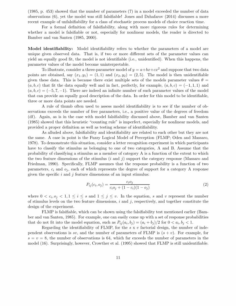
for a constant z > −1. Given that there are an infinite number of possible z values, there willbe an equally infinite number of parameter sets, each of which provides exactly the same fit tothe observed data. Figure 4 shows four selected sets of parameters obtained by applying the aboveequation. For example, given a parameter set, say c = (0.1, 0.3, 0.5, 0.7, 0.9), one can obtain anotherset c∗ = (0.36, 0.68, 0.83, 0.92, 0.98) for z = −0.8, or c∗ = (0.05, 0.18, 0.33, 0.54, 0.82) for z = 1. Notethat interestingly, the parameter values do change under the transformation in Eq. (3), but theirordinal relationships are preserved, in fact for all choices of the constant z (> −1). In short, giventhe unidentifiability of FLMP, one cannot meaningfully interpret the magnitudes of its parameters,except their ordinal structure.
Figure 4: Illustration of the unidentifiability of the FLMP model in Eq. (2). The curves show new sets of parameter
values, c∗’s and o∗’s, obtained by applying Eq. (3) for four different choices of the constant z.
Can FLMP be made identifiable? The answer is “yes.” For instance, one of its parameterscan be fixed to a preset constant (e.g., ck = 0.25, for some k). Alternatively, the model equationcan be modified to accommodate four response categories instead of two. For further details, thereader is referred to Crowther et al. (1995).
Model equivalency: This is a scarcely mentioned but important concept every cognitive modelershould be familiar with. For a given model equation, one can rewrite it in an equivalent formthrough a reparameterization of its parameters. As a concrete example of what is known as thereparametrization technique in statistics, consider a one-parameter exponential model defined as
12
y = e−ax where 0 < a < ∞. This model can be rewritten as y = bx, where 0 < b < 1, using thefollowing reparmetrization of the original parameter a: b = e−a.
To provide another and more substantive example of model equivalency, let us revisit themodel FLMP defined in Eq. (2). For this model, there exist at least two equivalent forms (e.g.,Crowther et al., 1995, pp. 404-405), and they are
Pij(αi, βj) =1
1 + e−(αi+βj), (αi = ln
ci1− ci
;βj = lnoj
1− oj) (4)
Pij(ui, vj) =1
1 + uivj, (ui =
1− cici
; vj =1− ojoj
)
where −∞ < αi, βj < ∞ and 0 < ui, vj < ∞. Note that Pij(αi, βj) = Pij(ui, vj) = Pij(ci, oj) forall pairs of (i, j).
It is important to note that different model forms created by reparametrization are equiva-lent to one another for all statistical and practical purposes. That is, the equivalent models wouldall fit any given data exactly the same, albeit with different values of their parameters, and wouldlead to exactly the same interpretation of, and conclusion from the data.
4.2 Model Estimation
Once data have been collected and the model is shown to be falsifiable and identifiable, one is ina position to assess the model’s goodness of fit to the experimental data. Recall that a model isdefined as a parametric family of probability distributions indexed by model parameters. Formally,model M = {f(y|θ) | θ ∈ Θ}, where y = (y1, ..., yn), θ = (θ1, ..., θk), and Θ is the parameter space.As such, the model contains many (theoretically infinite) probability distributions, each associatedwith a distinct set of parameter values. The main objective of model estimation is to find a setof parameter values that best fits the observed data in some defined sense–the procedure calledparameter estimation in statistics.
There are two generally accepted methods of parameter estimation (Myung, 2003): leastsquare estimation (LSE) and maximum likelihood estimation (MLE). In LSE, the parameter valuesthat minimize the sum of squared errors (SSE) between observations and predictions are sought:
SSE(θ) =n∑
i=1
(yi − yprd,i(θ))2 (5)
where yprd,i(θ) is the model’s prediction for observation yi. On the other hand, in MLE theparameter values that maximize the likelihood of the data, f(y|θ), or equivalently, the logarithmof the likelihood are sought:
ln f(y|θ) =n∑
i=1
ln f(yi|θ) (6)
under the assumption of independent observations. The parameter values that maximize MLEor minimizes MSE are usually sought numerically using optimization algorithms implemented oncomputer. The LSE solution tends to differ from the MLE solution unless all yi’s are normallydistributed with the same variance. MLE is generally a preferred method of parameter estimation,particularly in model comparison. From this point on, unless otherwise stated, we will assume that
13
a model’s goodness of fit is assessed by MLE, and the best-fitting parameter vector obtained inMLE is denoted by θ.
MLE is solely a method of model evaluation, not a method of model comparison. The latterrequires additional conceptualization and formalization, to which we now turn our attention.
4.3 Methods of Model Comparison
The trade-off between goodness-of-fit and complexity illustrated earlier is what makes model com-parison so difficult. The model must be complex enough to describe the variation in any datasample that is due to the underlying process, yet not overfit the data by absorbing noise and thuslosing generalizability. Conversely, the model must not be too simple to capture the underlyingprocess and thereby underfit the data, which will also lower generalizability. The goal of modelcomparison methods is to estimate a model’s generalizability by weighting fit against complexity.
In this section we provide a comprehensive overview of major methods of model comparisondeveloped to date, especially for modeling data in the behavioral and social sciences. We dividethem into three classes based on the approach. The first class of methods we discuss are penalized-likelihood methods, so called because they include a measure of fit along with one or more additionalterms that penalize the model for its complexity. The third class of methods are direct estimationmethods. As the name suggests, they are prescriptions for directly estimating generalizability, thusobviating the need to quantify fit and complexity independently. The second class of methods areBayesian comparison methods. We view them as a hybrids of the others. While some are Bayesianequivalents of penalized-likelihood measures, fit and complexity are not partialled out, making themfunctionally more akin to direct estimation methods.
For additional and complementary treatments of the topic, the interested reader shouldconsult three special journal issues on model comparison (Myung et al., 2000; Wagenmakers andWaldorp, 2006; Gluck et al., 2008), and recent review articles (Shiffrin et al., 2008; Vandekerckhoveet al., 2015).
4.3.1 Penalized-likelihood Methods
Among the many methods of model comparison, one class of methods that are those that makean appropriate adjustment to a model’s goodness of fit by separately quantifying complexity andcombinin it with a measure of fit.
Five representative methods that are currently in use are the Akaike Information Criterion(AIC; Akaike, 1973; Bozdogan, 2000), the second-order AIC (AICc; Hurvich and Tsai, 1989), theBayesian Information Criterion (BIC; Schwarz, 1978), the Fisher Information Approximation (FIA;Rissanen, 1996; Grunwald, 2000), and the Normalized Maximum Likelihood (NML; Rissanen, 2001;Myung et al., 2006).
14
They are defined as follows:
AIC = −2 ln f(y|θ) + 2k
AICc = −2 ln f(y|θ) + 2k +2k(k + 1)
n− k − 1
BIC = −2 ln f(y|θ) + k ln(n) (7)
FIA = − ln f(y|θ) +k
2ln
n
2π+ ln
∫
√
det(I(θ)) dθ
NML = − ln f(y|θ) + ln
∫
f(z|θ(z)) dz.
In the above equation, ln is the natural logarithm of base e, y = (y1, ..., yn) is a vector of observeddata, f(y|θ) is the maximum likelihood of the data, z is a vector variable of potential data, k and nare the number of free parameters and the sample size, respectively, and finally, I(θ) is the Fisherinformation matrix of sample size 1 (e.g., Schervish, 1995, p. 111).1 Note that the model withnormally distributed errors with a constant variance, the first term of AIC and BIC, −2 ln f(y|θ),can be replaced by (n ln(SSE) − n ln(n)) where SSE defined in Eq. (5) is the minimized sum ofsquared errors obtained by the method of least squares estimation (Burnham and Anderson, 2010,p. 63). Each of these five methods of model comparison prescribes that the model that minimizesa given criterion should be preferred.
Each of the criteria in the above equation consists of two factors. The first factor involving− ln f(y|θ) in the first term represents the lack of fit. The second factor that constitutes theremaining terms is naturally interpreted as model complexity. Model comparison in each criterionis carried out by trading lack-of-fit for complexity. A complex model with many parameters, havinga large value in the complexity factor, will not be chosen unless its fit justifies the extra complexity.It is in this sense that the model comparison criteria formalize the Principle of Occam’s Razor, whichstates, ”Entities must not be multiplied beyond necessity.” (William of Ockham, c. 1287-1347).
AIC, AICc and BIC: AIC originates from the information theory and has a distance inter-pretation. That is, AIC is derived as an asymptotic (i.e., large sample) approximation of theKullback-Leibler information divergence or distance between the true data-generating model andthe fitted model. As such, the model with the smallest value of AIC is the one that represents theclosest approximation to the truth. AICc, which is a variation of AIC, includes a small-sample biasadjustment term, and its use is recommended over AIC when the sample size (n) is relatively smallwith respect to the number of parameters (k), specifically, when n/k < 40 (Burnham and Anderson,2010, p. 66). BIC originates from Bayesian statistics, is derived as a large sample approximation ofBayesian Model Selection (BMS) described later in this chapter, and as such, the model with thesmallest value of this criterion is the one that is considered most likely to have generated observeddata.
The number of parameters is the only dimension of complexity that is considered by thesethree methods. As discussed earlier, functional form can also significantly affect model fit and
1For the model with a k-dim parameter vector θ = (θ1, ..., θk), the ij− th element of the Fisher information matrix
is defined as Iij(θ) = − 1nE(
∂2 ln f(y|θ)∂θi∂θj
)
, (i, j = 1, ..., k), where E denotes the statistical expectation with respect to
the probability density function f(y|θ). For an example calculation of I(θ) for retention models, the reader is directedto Pitt et al. (2002, pp. 488-490).
15
therefore needs to be taken into account in model comparison. The comparison methods introducednext are sensitive to functional form as well as the number of parameters.
It is important to note that AIC and AICc, as well as BIC for that matter, are on an intervalscale of measurement and thus should be interpreted accordingly. All that matters is the differencein AIC values, not the absolute values. In particular, the AIC differences can be transformedinto what are known as the Akaike weights that have probabilistic interpretations (Burnham andAnderson, 2010; Wagenmakers and Farrell, 2004). The Akaike weight for model Mi among a set ofm models being compared is defined as
wi(AIC) =exp
(
−12(AICi −AICmin)
)
∑mr=1 exp
(
−12(AICr −AICmin)
) , (i = 1, 2, ..,m) (8)
where AICmin is the minimum AIC value among the m models. The weight wi(AIC), as the weightof evidence in favor of model Mi, is interpreted as the probability that Mi is the one, among the setof the m candidate models, that minimizes the Kullback-Leibler information distance to the truedata-generating model (Burnham and Anderson, 2010, p. 75).
For AICc and BIC, one can also calculate the corresponding weights as was done for theAkaike weights in Eq. (8), and the resulting weights are interpreted in the same probabilisticmanner (Vandekerckhove et al., 2015).
Fisher Information Approximation (FIA): FIA was derived from the principle of MinimumDescription Length (MDL; Grunwald, 2007) in algorithmic coding theory in computer science.According to this principle, the goal of model comparison is to choose the model that permitsthe greatest compression of data in its description. The basic idea behind this approach is thata model, by definition, implies the presence of certain regularities, or equivalently redundancy, indata. That is, the more the data can be compressed using the redundancy extracted with thehelp of the model, the more we learn about the underlying regularities, and in turn, the better themodel generalizes as the extracted regularities will help the model make more accurate predictionsfor future observations.
As in the three methods of model comparison discussed above, the first term of FIA is alack of fit measure. The second and third terms together constitute the intrinsic complexity ofthe model. Importantly, and unique to FIA, the functional form dimension of model complexityis reflected through the Fisher information matrix I(θ) in the third term. That is, the Fisherinformation I(θ = (a, b, σ)) for the linear model defined as y = ax+ b+N(0, σ2) would be differentfrom that for the power model defined as y = axb + N(0, σ2). Additional examples of functionalform complexity can be found in Pitt et al. (2002) in which the influence of functional form onmodel comparison was demonstrated in three areas of cognitive modeling, namely, psychophysics,information integration, and category learning.
Finding the value of the third, functional-form complexity term can be challenging, thoughnot impossibly difficult. To do so, one would need first to obtain the Fisher information matrix,which is defined as the expectation of the second derivatives of the log-likelihood function withrespect to the parameter vector, and then to integrate the determinant of the resulting matrix overthe parameter space. Whereas the Fisher information can usually be obtained in analytic form,the integral must almost always be solved numerically using Monte Carlo methods (e.g., Robertand Casella, 2004). Concrete examples of the calculation of FIA that include the third term forselected models of cognition can be found in these sources (Su et al., 2005; Wu et al., 2010a; Klauer
16
and Kellen, 2011; Kellen and Klauer, 2011; Singmann and Kellen, 2013; Klauer and Kellen, 2015).Again, regarding the third term of FIA, it is worth noting that this term does not depend
upon the sample size n, and therefore, as the sample size increases, its relative contribution tomodel complexity becomes negligible in comparison to that of the second term, which is a loga-rithmic function of n. Consequently, for sufficiently large n, FIA is reduced essentially to BIC, i.e.,approximately one half of it.
Normalized Maximum Likelihood (NML): Like FIA, NML is also motivated from the sameMDL principle. The two methods are related to each other such that FIA is derived as an asymptoticapproximation to NML (e.g., Barron et al., 1998; Myung et al., 2006), and importantly, NMLrepresents a full solution to a minimax problem of inductive inference (Rissanen, 1996, 2001), aswe discuss in what follows.
Specifically, given the model f(y|θ) under consideration, the minimax problem is defined asfinding one probability distribution g∗(y) that minimizes its maximum distance to the best-fittingmember, i.e., f(y|θ(y)), of the parametric family of the model where the data y are generated fromanother probability distribution h(y):
g∗(y) = argming
maxh
Eh
[
lnf(y|θ(y))
g(y)
]
. (9)
In the above equation, θ(y) is the maximum likelihood estimate obtained by MLE, and g andh range over the set of virtually all probability distributions and are not required to belong tothe model family under consideration. Note that the distance Eh [·] is measured by the Kullback-Leibler information divergence between two distributions, f(y|θ(y)) and g(y) where the expectationis taken with respect to the data generating distribution h(y), but not f(y|θ(y)) as it would bedone normally.
The solution to the minimax problem (Rissanen, 2001) is obtained as
g∗(y)f(y|θ(y))
∫
f(z|θ(z)) dz. (10)
This optimal distribution assigns a probability number to each data vector y that is proportional tothe maximized likelihood value f(y|θ(y)) and divided by the normalizing constant,
∫
f(z|θ(z)) dz,so that it becomes a proper probability density function satisfying
∫
g∗(y) dy = 1. As such, g∗(y) iscalled the normalized maximum likelihood (NML) distribution. Note that the normalizing constantis the sum of maximum likelihood values of all possible data vectors that could potentially beobserved in a given experimental setting.
The NML criterion in Eq. (7) is then obtained from Eq. (10) by taking the minus loga-rithm such that NML := − ln g∗(y). Accordingly, the lower the NML criterion value, the higherprobability the NML distribution assigns to the observed data.
How should we interpret the NML distribution and likewise the NML criterion? First of all,the idea behind the minimax problem in Eq. (9) which both are derived from is that we wish toidentify and adopt one probability distribution as a representative of the entire model family. Fromthe way the minimax problem is set up in Eq. (9), it follows that the representative distribution asa solution to the minimax problem is sought as the one that most closely mimics the the model’s
17
data-fitting behavior under virtually all practical situations–that is, for all possible data generatedby all kinds of models–even including the case in which the data may not come from the modelunder consideration, i.e., under model misspecification. Further, the solution g∗(y) is not evenrequired to be a member of the model family. As such, the minimmax problem encapsulates aminimalist and pragmatic approach to model comparison. Accordingly and deservingly, we believethat NML, as the solution to the minimax problem, is one of the most complete and robust methodsof model comparison the field has to offer.
Now let us examine carefully the normalizing constant of the NML distribution in Eq. (10),which is defined as the sum of all best fits the model can provide collectively for all possible datapatterns. The logarithm of this constant corresponds to the complexity penalty term of the NMLcriterion in Eq. (7). Therefore, a complex model is the one that fits well a wide range of datapatterns, regardless of whether they are empirically observable or not. It is in this sense thatthe normalizing constant captures our intuition about model complexity, that is, “the flexibilityinherent in a model that enables it to fit diverse patterns of data” (Myung and Pitt, 1997, p. 80).In short, from the NML standpoint, a model to be favored is the one that provides an excellentfit to the observed data but does poorly otherwise, in accordance with the notion of a “good andpersuasive” fit (Roberts and Pashler, 2000, Fig. 1).
Finally, as is the case with FIA, the calculation of the complexity term of the NML criterioncan be challenging given that it involves an integration over the data space. Concrete examples ofcalculating this term can be found in recent articles (e.g., Su et al., 2005; Wu et al., 2010b; Klauerand Kellen, 2011; Kellen and Klauer, 2011; Klauer and Kellen, 2015).
4.3.2 Bayesian Methods
Bayesian methods of model comparison were developed as a Bayesian alternative to the frequentist-oriented methods such AIC. The attractions of Bayesian statistics in general are many and include:(1) subjectivity of uncertainty quantification (degree-of-personal-belief interpretation of probabil-ity); (2) directness of inference (direct estimation of the probability of an unknown quantity); (3)cumulative nature of inference (combining a prior belief and data using Bayes rule to form a newupdated belief, which in turn serves as a prior in the next cycle); and (4) ease of computation(Markov chain Monte Carlo makes it possible to simulate effortlessly any arbitrary posterior distri-bution). It is then no surprise that we have recently witnessed a significant and dramatic increase inthe interest and practice of Bayesian modeling in social and behavioral sciences (Lancaster, 2004;Lynch, 2007; Gill, 2008; Kaplan, 2014; Kruschke, 2014; Lee and Wagenmakers, 2014). These inturn naturally create the issue of comparing among Bayesian models of the phenomenon underinvestigation. In this section, we review two commonly used methods, the Bayesian factor (BF)and the deviance information criterion (DIC).
Bayesian Model Selection (BMS): BMS is the principal method of model comparison inBayesian inference. The goal of BMS is to select the one model, among the set of candidatemodels, that is most likely to have generated observed data. This is achieved by minimizing thecriterion value defined as:
BMS = − ln
∫
f(y|θ) p(θ) dθ, (11)
where f(y|θ) is the likelihood function and p(θ) is the (parameter) prior. The integral on the right-hand side of the equation is called the marginal likelihood, denoted by p(y) =
∫
f(y|θ) p(θ) dθ.
18
That is, BMS is equal to the minus logarithm of the marginal likelihood. The method prescribesthat the model with the smallest BMS should be preferred.
The difference in BMS between two models, M1 and M2, is related directly to the Bayesfactor (BF; Kass and Raftery, 1995). The Bayes factor is defined as the ratio of the marginallikelihood under one model to that under the other model, i.e., BF12 = p(y|M1)/p(y|M2)). Suchas, the following equation shows the relationship between BMS and BF:
BMS2 −BMS1 = lnBF12 (12)
= lnp(M1|y)
p(M2|y)
The last equality above is from Bayes rule, p(M1|y)p(M2|y)
= p(M1)p(M2)
× BF12, under the assumption of
equal model priors, i.e., p(M1) = p(M2). It is then straightforward to express a model’s posteriorprobability in terms of its BMS value as:
p(Mi|y) =e−BMSi
∑mj=1 e−BMSj
, (i = 1, ...,m) (13)
for a set of m models being compared. In short, the smaller the BMS value of a model, thegreater the model’s posterior probability. It is in this sense that minimization of BMS amounts tomaximization of the posterior model probability.
Now, we make several important observations about BMS.First, note that the marginal likelihood, p(y) =
∫
f(y|θ) p(θ) dθ, from which BMS is derivedis simply the weighted mean of the likelihood f(y|θ) across the parameter space with the prior p(θ)as the weight. It is this mean likelihood that allows BMS to avoid overfitting, unlike the maximumlikelihood that is a GOF measure and thus is necessarily susceptible to the problem. In otherwords, BMS is equipped with a built-in complexity penalization to safeguard against overfitting,thereby ensuring good generalizability.
Second and interestingly, the exact form of FIA in Eq. (7) is obtained from an asymptoticexpansion of BMS under the Jeffreys prior (Balasubramanian, 1997, 2005; Myung et al., 2006).This “surprising” connection between the two seemingly disparate theoretical frameworks (i.e.,algorithmic coding theory of data compression versus Bayesian theory of statistical inference) pointsto a future and potentially fruitful area of research. Related and as noted earlier, BMS is reducedto one half of BIC for large sample size n (Raftery, 1993).
Third, as is the case for FIA and NML, BMS can be nontrivial to compute due to itsintegral expression. The integral is generally not amenable to an analytic solution, and therefore,often must be solved numerically using Monte Carlo techniques.
Finally and importantly, it turns out that the calculation of BMS and so BF is considerablysimplified for comparison with nested models. A model is said to be nested with another model ifthe former is obtained from the latter by fixing the values of one or more parameters of the latter.For example, a model defined y = at is nested within another model defined as y = at+bt2+c sincethe former model is obtained by fixing b = c = 0 in the latter model. Specifically and formally, letus consider two nested models, M1 and M2, in which model M1 has a parameter vector θ and modelM2 has an extra parameter vector φ such that M1 corresponds to M2 with φ = φ0 for some fixedconstant φ0. To illustrate, in the example just discussed, the notation translates to M1 : y = at,M2 : y = at+ bt2 + c, θ = (a), φ = (b, c), and φ0 = (0, 0). In any case, the BF for M1 versus M2
19
simply becomes the ratio of the posterior to prior density values under M2 at φ = φ0:
BF12 =p(y|M1)
p(y|M2)=
p(φ = φ0|y,M2)
p(φ = φ0|M2). (14)
The above ratio is known as the Savage-Dickey density ratio (Dickey, 1971; O’Hagan and Forster,2004, pp. 174-177). This Savage-Dickey method is especially useful in Bayesian hypothesis testingwith equality and inequality constraints (e.g., H0: µ = 0 vs H1: µ 6= 0; H0: µ = 0 vs H1: µ > 0).For in-depth treatments of the topic with concrete example applications in cognitive modeling, thereader is advised to read these excellent sources (Wagenmakers et al., 2010; Wetzels et al., 2010;Lee and Wagenmakers, 2014).
Deviance Information Criterion (DIC): DIC (Spiegelhalter et al., 2002; Gelman et al., 2013)is a Bayesian analog of AIC defined as
DIC = −2 ln f(y|θ) + 2pD. (15)
In the above equation, f(y|θ) is the likelihood evaluated at the posterior mean θ (i.e., mean of theposterior distribution, p(θ|y)), and pD is a model complexity measure called the effective numberof parameters:
pD = 2 ln f(y|θ)− 2Eθ|y [ ln f(y|θ) ] , (16)
where the expectation E[·] in the second term is taken with respect to p(θ|y).2
There are a few things worth mentioning about DIC. First, note the similarity betweenDIC and AIC in Eq. (7): the former is obtained from the latter by first substituting the maximumlikelihood estimate θ for the posterior mean θ and then substituting the number of parameters kfor the effective number of parameters pD. Second, DIC is a predictive accuracy measure, the goalof which is to identify a model that achieves best predictions for future observations. Third, theeffective number of parameters, pD, takes on a continuous positive value and is sensitive to thenumber of parameters and also importantly, the functional form. Lastly, the calculation of DIC isroutine and straightforward; all that is required are samples drawn from the posterior distribution,which can be done using Markov chain Monte Carlo (MCMC: e.g., Brooks et al., 2011). This isunlike BMS and BF, for which an easy-to-implement and general-purpose computational algorithmhas yet to be developed. The latter two properties of DIC, in particular, make the criterionwell-suited for its usage in hierarchical Bayesian modeling that has recently become increasinglypopular in cognitive modeling (e.g., Rouder and Lu, 2005; Lee, 2011; Lee and Wagenmakers, 2014).Many software packages including BUGS (Spiegelhalter et al., 2003) and JAGS (http://mcmc-jags.sourceforge.net) provide DIC values for hierarchical as well as non-hierarchical models.
Before closing, we should mention two other Bayesian criteria, each of which represents animprovement on DIC. They are the Bayesian Predictive Information Criterion (BPIC; Ando, 2007)and the Watanabe-Akaike Information Criterion (WAIC; Watanabe, 2010). BPIC improves uponDIC in that it does not require, as does DIC, the assumption that the model is correctly specified(i.e., containing the true, data-generating process). On the other hand, WAIC is a Bayesian analogof LOOCV that is reparametrization-invariant (DIC is not) (Spiegelhalter et al., 2002, p. 612).The Bayesian package Stan (http://mc-stan.org) provides WAIC values.
2DIC can be expressed in another equivalent form as DIC = D + pD, where D = −2Eθ|y [ ln f(y|θ) ].
20
4.3.3 Direct Estimation Methods
In this third section we introduce methods in which we obtain directly a sample-based estimateof a model’s generalizability, without relying upon an explicit measure of complexity. This directestimation of generalizability is achieved by simulating procedurally the two steps of data collectionand model prediction, separately one at a time. The exact details of how this is done depend uponthe specific method chosen.
Cross Validation (CV): This is probably the most popular method of model comparison withinthe class of direct estimation methods (e.g., Stone, 1974; Browne, 2000). In CV, we first randomlydivide the observed data sample into two sub-samples of equal size, calibration (ycal) and validation(yval). We then use the calibration sample to obtain the best-fitting parameter values of the modelby maximum likelihood estimation. These values, denoted by θ(ycal) are then applied directlywithout further parameter tuning to fit the validation sample to obtain the model’s predictionaccuracy, which is taken as an estimate of the model’s generalizability.
The specific CV criterion can be expressed using an appropriate fit measure such as theminus log-likelihood or the root mean squared error. In terms of the former, CV is defined asfollows:
CVsplit−half = − ln f(yval|θ(ycal)), (17)
which is actually an index of the lack of generalizability. Accordingly, the model with the smallestCV value should be chosen as the best generalizing model. This particular method of cross valida-tion is known as the split-half CV. One issue is that the resulting CV value would depend on howthe calibration and validation samples are selected. This sampling dependency can be minimizedby repeatedly performing half-split CV for a large number of splits, each randomly chosen, andthen calculating the average CV value as a model’s generalizability measure.
There is another method of cross-validation called as the leave-one-out-cross-validation(LOOCV) that by construct avoids the sampling dependency problem in split-half CV. Specifi-cally, in LOOCV, each of the n observations in a data set serves as the validation sample, withthe remaining (n − 1) observations serving as the calibration sample. The standard calibration-validation step is repeated for all observations, exactly n times. The model’s generalizability isthen estimated as the average of n minus log-likelihoods as
LOOCV = −1
n
n∑
i=1
ln f(yi|θ(y 6=i)). (18)
In the above equation, y 6=i denotes the calibration sample consisting of (n−1) observations excludingyi, which itself is treated as the validation sample. A schematic diagram of how LOOCV worksis illustrated in the left panel of Figure 5. It is worth noting that LOOCV is related to AIC suchthat model choice under both criteria is asymptotically equivalent provided that certain regularityconditions are met (Stone, 1977).
Cross validation somehow takes into account the effects of both dimensions of model com-plexity (the number of parameters and functional form), though how this is accomplished is notclear. It is therefore not possible to get an explicit measure of model complexity. The methodis equally applicable to comparing formal statistical models and non-formal models without likeli-
21
Figure 5: Schematic illustration of the differences between LOOCV and APE. Each plain box represents a single
observation. The plain boxes with the bold outline represent the calibration sample whereas the scratched box
represents the validation sample. The plain boxes with the light dotted line in the right panel are not being used as
part of the calibration-and-validation step.
hoods, such as connectionist models and simulation-based models. In short, its ease of implementa-tion and versatility make cross validation a highly attractive and recommendable method of modelcomparison.
Generalization Criterion (GC): This criterion, due to Busemeyer and Wang (2000), has beenproposed as a formal implementation of the strong inference test (Platt, 1964) and is similar tocross validation, at least in sprit if not in substance. The basic idea of GC is to compare andchoose among alternative explanations (models) of the phenomenon of interest based on their “apriori predictions (made before observing data) rather than post hoc fits (made after observingthe data)” (Busemeyer and Wang, 2000, p. 172). Specifically, in GC, the complete experimentaldesign is partitioned into two subdesigns, a calibration design and a generalization design. The firstpartition is used to estimate a model’s best-fitting parameter values, which in turn without furtherparameter tuning are used to compute the new predictions for the second, generalization-designpartition. The model, among a set of candidate models, that makes the most accurate predictionsunder an appropriate fit measure is preferred. Ahn et al. (2008) provides an example applicationof GC in cognitive modeling.
Despite the apparent similarity between the two, the generalization criterion differs in aimportant way from cross validation: In GC, models are evaluated in their ability to generalizeto new and importantly, different experimental design or tasks.3 Note that in CV or LOOCV as
3For instance, a decision scientist might be interested in how well the parameter values of a risky choice modelestimated based on current observations from a decision-from-description (DFD) task can account for new, futureobservations from another and different decision-from-experience (DFE) task. In the DFD task, the participant isasked to choose between two fictitious gambles with probabilities of rewards described in an explicit numerical form.
22
well as in other methods of model comparison for that matter, the goal is to estimate a model’sgeneralizability from one sample data to another sample data, both of which are drawn from thesame experimental task or design setting.
In summary, GC is conceptually intuitive and easy to understand and use. In our view, GCrepresents a major step towards extending the current theory of model comparison to a more generaland scientifically relevant goal. Unlike the other methods of model comparison we reviewed in thepresent chapter, however, the theoretical foundation of GC is not well understood and established.For example, it is not entirely clear what the criterion is designed to achieve theoretically. How doesit take into account model complexity so as to avoid overfitting? In what sense is it an “optimal”method of model comparison? How does it behave asymptotically?
Accumulative Prediction Error (APE): This is another direct estimation method in whicha model’s generalizability is estimated in an accumulative fashion under the premise that the dataarrive in a sequentially ordered stream (Dawid, 1984; Wagenmakers et al., 2006).
Specifically, for a given model with k parameters and a data set of n observations, we fitthe model to the first (k+1) observations as a calibration sample, obtain the maximum likelihoodestimate, and then treat the (k + 2) − th observation as a validation sample of size 1 to estimatethe model’s generalizability measured by its prediction accuracy for the validation sample. In thisfirst round of calibration-validation split, we have used just the first (k+2) observations out of thetotal of n observations in the data. In the next round, the calibration sample increases in size byone by taking in the (k + 2) − th observation, and the (k + 3) − th observation now becomes thevalidation sample. The accumulative process is repeated until we arrive at the n− th observationas the validation sample, as illustrated in the right panel of Figure 5.
Formally, the APE criterion is defined as the average of a total of (n − k − 1) individualgeneralizability estimates:
APE = −1
(n− k − 1)
n∑
i=k+2
ln f(yi|θ(y1, y2, ..., yi−1)). (19)
The method prescribes that the model with the lowest APE value should be preferred as the bestgeneralizing model.
Like CV and LOOCV discussed earlier, APE is easy to implement and takes into account,though implicitly, the effects of both the number of parameters and functional form dimensionsof model complexity, and therefore is highly recommended for all model comparison situations.Further, APE and BIC are related to each other such that they are asymptotically equivalentunder certain conditions (Dawid, 1984, p. 288).
On the other hand, in the DFE task, the participant is not given the probability information and instead, must learnthe probabilities in an experiential manner, i.e., by observing the outcomes of the chosen gambles over choice trials(e.g., Hertwig and Erev, 2009).
23
Figure 6: Best-fits of the four models of retention memory in Eq. (20) to an artificial data set. The solid circles
represent the data.
4.4 Illustrated Example
In this section we illustrate the use of six comparison methods in assessing the same four modelsof memory retention as in Table 1. They are defined as
LIN : p(θ = (a, b), t) = at+ b
EXP : p(θ = (a, b), t) = ae−bt (20)
POW : p(θ = (a, b), t) = a(t+ 1)−b
EXPOWS : p(θ = (a, b, c, d, e, f), t) = ae−bt + c(t+ 1)−dsin(et) + f
Each model was fitted by maximum likelihood estimation (MLE) to an artificial data set of 21binomial counts (n = 21) of successes out of 50 Bernoulli trials (N = 50) for the same 21 retentionintervals as those used in Table 1.4 Figure 6 shows the best-fits of the four models.
4The data vector of 21 counts was y = (48, 42, 29, 34, 23, 26, 23, 19, 14, 19, 14, 14, 10, 15, 9, 8, 6, 10, 3, 8, 1).
24
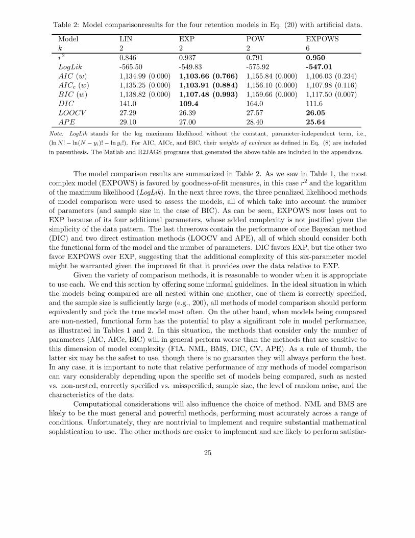
Table 2: Model comparisonresults for the four retention models in Eq. (20) with artificial data.
Note: LogLik stands for the log maximum likelihood without the constant, parameter-independent term, i.e.,
(lnN !− ln(N − yi)!− ln yi!). For AIC, AICc, and BIC, their weights of evidence as defined in Eq. (8) are included
in parenthesis. The Matlab and R2JAGS programs that generated the above table are included in the appendices.
The model comparison results are summarized in Table 2. As we saw in Table 1, the mostcomplex model (EXPOWS) is favored by goodness-of-fit measures, in this case r2 and the logarithmof the maximum likelihood (LogLik). In the next three rows, the three penalized likelihood methodsof model comparison were used to assess the models, all of which take into account the numberof parameters (and sample size in the case of BIC). As can be seen, EXPOWS now loses out toEXP because of its four additional parameters, whose added complexity is not justified given thesimplicity of the data pattern. The last threerows contain the performance of one Bayesian method(DIC) and two direct estimation methods (LOOCV and APE), all of which should consider boththe functional form of the model and the number of parameters. DIC favors EXP, but the other twofavor EXPOWS over EXP, suggesting that the additional complexity of this six-parameter modelmight be warranted given the improved fit that it provides over the data relative to EXP.
Given the variety of comparison methods, it is reasonable to wonder when it is appropriateto use each. We end this section by offering some informal guidelines. In the ideal situation in whichthe models being compared are all nested within one another, one of them is correctly specified,and the sample size is sufficiently large (e.g., 200), all methods of model comparison should performequivalently and pick the true model most often. On the other hand, when models being comparedare non-nested, functional form has the potential to play a significant role in model performance,as illustrated in Tables 1 and 2. In this situation, the methods that consider only the number ofparameters (AIC, AICc, BIC) will in general perform worse than the methods that are sensitive tothis dimension of model complexity (FIA, NML, BMS, DIC, CV, APE). As a rule of thumb, thelatter six may be the safest to use, though there is no guarantee they will always perform the best.In any case, it is important to note that relative performance of any methods of model comparisoncan vary considerably depending upon the specific set of models being compared, such as nestedvs. non-nested, correctly specified vs. misspecified, sample size, the level of random noise, and thecharacteristics of the data.
Computational considerations will also influence the choice of method. NML and BMS arelikely to be the most general and powerful methods, performing most accurately across a range ofconditions. Unfortunately, they are nontrivial to implement and require substantial mathematicalsophistication to use. The other methods are easier to implement and are likely to perform satisfac-
25
torily under restricted conditions. For example, when models have the same number of parametersbut differ in functional form, DIC, CV, and APE are recommended because unlike AIC, AICc orBIC, they are sensitive to the functional form dimension of complexity. If models differ only innumber of parameters and the sample size relatively large, then AIC, AICc and BIC should do agood job.
5 Conclusion
In this chapter we have reviewed many model comparison methods. Some, such as AIC and CV,are in wide use across disciplines, whereas others, such as NML, are newer and their adoption islikely to be stymied by the challenges of implementation. That so many different methods exist forcomparing models speaks to the ubiquity and importance of the enterprise. Data are our only linkto the cognitive processes we investigate. They are thus priceless in advancing our understanding,which includes choosing among alternative explanations (models) of those data. This is particularlytrue when evaluating a model’s ability to predict the data from a new experiment, one that is afresh test of model behavior rather than data generated in past experiments (Smolin, 2006).
The focus of this chapter on quantitative and statistical methods of model comparisonshould not be taken to imply that they are the most important criteria in determining modeladequacy or superiority. They are but one type of information that the researcher should use.Qualitative and non-statistical criteria of model evaluation can be just as or even more important,especially in the early stages of model development and during model revision. For example,plausibility (sound assumptions), explanatory adequacy (principled account of the process) andmodel faithfulness (model behavior truly stems from the theoretical principles it embodies) arefoundational criteria that must be satisfied to take a model seriously. Otherwise one possesses astatistical model, or at best a nonsensical cognitive model.
Heavy or exclusive reliance on comparison techniques, however sophisticated, can be ill-advised when one is splitting hairs in choosing among models. When models mimic each other,accounting of the same list of behavioral or neurophysiological data similarly well, efforts shouldfocus on designing experiments that can differentiate the models more clearly, or concede that themodels are functionally isomorphic and thus indistinguishable. Of course, it is not easy to designa clever experiment that can decisively differentiate one model from another, but we believe it isultimately the more productive path to follow. The results from a discriminating experimentaldesign will usually be more persuasive than a large Bayes Factor, for example. As we have notedelsewhere (Navarro et al., 2004), model comparison methods are limited by the informativeness ofthe data collected in experiments, so anything that can be done to improve data quality shouldbenefit the research enterprise. Readers interested in this topic should consult writings on optimalexperimental design (Myung and Pitt, 2009; Myung et al., 2013).
In closing, model comparison methods are but one tool that can be used to guide modelselection. They seek to maximize generalizability under the belief that it is the best known wayto capture the regularities of a noisy system. Although they vary widely in theoretical orientation,ease of implementation, and comprehensiveness, they are functionally similar in that they evaluatethe match between the complexity of the data and the corresponding complexity of the models.The model for which this match is optimal should be preferred.
26
6 Acknowledgement
The authors wish to thank Hairong Gu for his helpful comments on earlier drafts of the chapter.
7 Appendix A: Matlab Code for Illustrated Example
This appendix includes the Matlab code that generated the simulation results for AIC, AICc, BIC,LOOCV and APE in Table 2.
Ahn, W., Busemeyer, J. R., Wagenmakers, E.-J., and Stout, J. (2008). Comparison of decisionlearning models using the generalization criterion method. Cognitive Science, 32:1376–1402.
Akaike, H. (1973). Information theory and an extension of the maximum likelihood principle. InPetrov, B. N. and Caski, F., editors, Proceedings of the Second International Symposium onInformation Theory, pages 267–281, Budapest. Akademiai Kiado.
Anderson, J. R. and Lebiere, C. (1998). The Atomic Components of Thought. Lawrence ErlbaumAssociates, Mahwah, NJ.
Ando, T. (2007). Bayesian predictive information criterion for the evaluation of hierarchicalBayesian and empirical Bayes models. Biometrika, 92(2):443–458.
Balasubramanian, V. (1997). Statistical inference, occam’s razor and statistical mechanics on thespace of probability distributions. Neural Computation, 9:349–368.
Balasubramanian, V. (2005). Mdl, Bayesian inference, and the geometry of the space of probabilitydistributions. In Grunwald, J., Myung, I. J., and Pitt, M. A., editors, Advances in MinimumDescription Length, chapter 3, pages 81–98. MIT Press.
Bamber, D. and van Santen, J. (1985). How many parameters can a model have and still betestable. Journal of Mathematical Psychology, 29:443–473.
Bamber, D. and van Santen, J. (2000). How to assess a model’s testability and identifiability.Journal of Mathematical Psychology, 44:20–40.
Barron, A. R., Rissanen, J., and Yu, B. (1998). The minimum description length principle in codingand modeling. IEEE Transactions on Information Theory, 44:2743–2760.
Bollen, K. A. (1989). Structural Equation with Latent Variables. John Wiley & Sons, New York,NY.
Box, G. E. P. (1976). Science and statistics. Journal of the American Statistical Association,71(356):791–799.
Bozdogan, H. (2000). Akaike information criterion and recent developments in information com-plexity. Journal of Mathematical Psychology, 44:62–91.
Brooks, S., Gelman, A., Jones, G. L., and Meng, X.-L., editors (2011). Handbook of Markov ChainMonte Carlo. CRC Press, Boca Raton, FL.
Browne, M. W. (2000). Cross-validation methods. Journal of Mathematical Psychology, 44:108–132.
Burnham, K. P. and Anderson, D. R. (2010). Model Selection and Multi-Model Inference: APractical Information-Theoretic Approach (2nd edition). Springer, New York, NY.
35
Busemeyer, J. R. and Wang, Y. (2000). Model comparisons and model selections based on gener-alization criterion methodology. Journal of Mathematical Psychology, 44:171–189.
Crowther, C. S., Batchelder, W. H., and Hu, X. (1995). A measurement-theoretic analysis of thefuzzy logical model of perception. Psychological Review, 102:396–408.
Dawid, A. P. (1984). Present position and potential developments: Some personal views: Statisticaltheory: The prequential approach. Journal of the Royal Statistical Society, Series A, 147:278–292.
Dickey, J. M. (1971). The weighted likelihood ratio, linear hypotheses on normal location parame-ters. Annals of Mathematical Statistics, 42:204–223.
Fum, D., Del Missier, F., and Stocco, A. (2007). The cognitive modeling of human behavior: Whya model is (sometimes) better than 10,1000 words. Cognitive Systems Research, 8:135–142.
Gelman, A., Carlin, J. B., Stern, H. S., Dunson, D. B., Vehtari, A., and Rubin, D. B. (2013).Bayesian Data Analysis. Chapman & Hall/CRC, Boca Raton, Florida, third edition.
Gill, J. (2008). Bayesian Methods: A Social and Behavioral Sciences Approach. ChapmanHall/CRC, Boca Raton, FL, second edition.
Gluck, K., Bello, P., and Busemeyer, J. (2008). Introduction to the special issue. Cognitive Science,32(8):1245–1247.
Gries, S. T. (2015). The most under-used statistical methods in corpos linguistics: multi-level (andmixed-effects) models. Corpora, 10(1):95–125.
Grunwald, P. D. (2000). Model selection based on minimum description length. Journal of Math-ematical Psychology, 44:133–152.
Grunwald, P. D. (2007). The Minimum Description Length Principle. M.I.T. Press.
Hambleton, R. K., Swaminathan, H., and Rogers, H. J. (1991). Fundamentals of Item ResponseTheory. Lawrence Erlbaum Associates, Newbury Park, CA.
Hertwig, R. and Erev, I. (2009). The description-experience gap in risky choice. Trends in CognitiveSciences, 13(12):517–523.
Hurvich, C. M. and Tsai, C.-L. (1989). Regression and time series model selection in small samples.Biometrika, 76:297–307.
Jacobs, A. M. and Grainger, J. (1994). Models of visual word recognition–sampling the state of theart. Journal of Experimental Psychology: Human Perception and Performance, 29:1311–1334.
Jones, M. and Dzhafarov, E. N. (2014). Unfalsifiability and mutual translatability of major modelingschemes for choice reaction time. Psychological Review, 121(1):1–32.
Kaplan, D. (2014). Bayesian Statistics for the Social Sciences. Guilford Press, New York, NY.
Kass, R. E. and Raftery, A. E. (1995). Bayes factors. Journal of the American Statistical Associa-tion, 90:773–795.
36
Kellen, D. and Klauer, K. C. (2011). Evaluating models of recognition memory using the first- andsecond-choice responses. Journal of Mathematical Psychology, 55:251–266.
Klauer, K. C. and Kellen, D. (2011). The flexibility of models of recognition memory: An analysisby the minimum-description length principle. Journal of Mathematical Psychology, 55:430–450.
Klauer, K. C. and Kellen, D. (2015). The flexibility of models of recognition memory: The case ofconfidence ratings. Journal of Mathematical Psychology, 67:8–25.
Kruschke, J. K. (2014). Doing Bayesian Data Analysis: A Tutorial with R, JAGS, and stan.Academi Press, New York, NY, second edition.
Lancaster, T. (2004). An Introduction to Modern Bayesian Econometrics. Blackwell Publishing,Malden, MA.
Lee, M. D. (2011). How cognitive modeling can benefit from hierarchical Bayesian models. Journalof Mathematical Psychology, 55(1):1–7.
Lee, M. D. and Wagenmakers, E.-J. (2014). Bayesian Cognitive Modeling: A Practical Course.Cambridge University Press, Cambridge, U.K.
Lewandowsky, S. (1993). The rewards and hazards of computer simulations. Psychological Science,4:236–243.
Lewandowsky, S. and Farrell, S. (2011). Computational Modeling in Cognition: Principles andPractice. Sage Publications, Thousand Oaks, CA.
Luce, R. D. (1956). Individual Choice Behavior. Wiley, New York: NY.
Lynch, S. M. (2007). Introduction to Applied Bayesian Statistics and Estimation for Social Scien-tists. Springer, New York, NY.
Massaro, D. W. and Friedman, D. (1990). Models of integration given multiple sources of informa-tion. Psychological Review, 97:225–252.
McClelland, J. L. (2009). The place of modeling in cognitive science. Topics in Cognitive Science,1:11–38.
Myung, I. J. (2000). The importance of complexity in model selection. Journal of MathematicalPsychology, 44(4):190–204.
Myung, I. J. (2003). Tutorial on maximum likelihood estimation. Journal of Mathematical Psy-chology, 47:90–100.
Myung, I. J., Brunsman, A. E., and Pitt, M. A. (1999). True to thyself: Assessing whethercomputational models of cognition remain faithful to their theoretical principles. In Hahn, M.and Stoness, S., editors, Proceedings of the 21st Annual Conference of the Cognitive ScienceSociety, pages 462–467, Mahwha, N.J. Lawrence Erlbaum Associates.
Myung, I. J., Forster, M., and Browne, M. W. (2000). Special issue on model selection. Journal ofMathematical Psychology, 44:1–2.
37
Myung, I. J. and Pitt, M. A. (1997). Applying Occam’s razor in modeling cognition: A Bayesianapproach. Psychonomic Bulletin & Review, 4:79–95.
Myung, I. J. and Pitt, M. A. (2002). Mathematical modeling. In Wixted, J., editor, Stevens’Handbook of Experimental Psychology, Volume IV: Methodology, pages 429–459, New York, NY.John Wiley & Sons.
Myung, J. I., Cavagnaro, D. R., and Pitt, M. A. (2013). A tutorial on adaptive design optimization.Journal of Mathematical Psychology, 57:53–67.
Myung, J. I., Cavagnaro, D. R., and Pitt, M. A. (2016). Model evaluation and selection. InBatchelder, W. H., Colonius, H., Dzhafarov, E., and Myung, J. I., editors, New Handbook ofMathematical Psychology, Volume I: Measurement and Methodology, pages 000–000, Cambridge,UK. Cambridge University Press.
Myung, J. I., Navarro, D. J., and Pitt, M. A. (2006). Model selection by normalized maximumlikelihood. Journal of Mathematical Psychology, 50:167–179.
Myung, J. I. and Pitt, M. A. (2009). Optimal experimental design for model discrimination.Psychological Review, 58:499–518.
Navarro, D. J., Pitt, M. A., and Myung, I. J. (2004). Assessing the distinguishability of modelsand the informativeness of data. Cognitive Psychology, 49:47–84.
Oden, G. C. and Massaro, D. W. (1978). Integration of featural information in speech perception.Psychological Review, 85:172–191.
O’Hagan, A. and Forster, J. (2004). Kendall’s Advanced Theory of Statistics, volume 2B: BayesianTheory. Arnold, London, UK, second edition.
Pitt, M. A., Myung, I. J., and Zhang, S. (2002). Toward a method of selecting among computationalmodels of cognition. Psychological Review, 190(3):472–491.
Platt, J. R. (1964). Strong inference: Certain systematic methods of scientific thinking may producemuch more rapid progress than others. Science, 146(3642):347–353.
Plaut, D. C., McClelland, J. L., and Seidenberg, M. S. (1996). Understanding normal and im-paried qord reading: Computational principles in quasi-regular domains. Psychological Review,103(1):56–115.
Popper, K. R. (1959). The Logic of Scientific Discovery. Basic Books, New York: NY.
Preacher, M. J. (2006). Quantifying parsimony in structural equation modeling. MultivariateBehavioral Research, 41(3):227–259.
Raftery, A. E. (1993). Bayesian model selection in structural equation models. In Bollen, K. andLong, J. S., editors, Testing Structural Equation Models, pages 163–180. Sage Publications.
Rissanen, J. (1996). Fisher information and stochastic complexity. IEEE Transactions on Infor-mation Theory, 42:40–70.
38
Rissanen, J. (2001). Strong optimality of the normalized ml models as universal code and informa-tion in data. IEEE Transactions on Information Theory, 42:1712–1717.
Robert, C. P. and Casella, G. (2004). Monte Carlo Statistical Methods. Springer, New York, NY,second edition.
Roberts, S. and Pashler, H. (2000). How pursuasive is a good fit? a comment on theory testing.Psychological Review, 107:358–367.
Rouder, J. N. and Lu, J. (2005). An introduction to Bayesian hierarchical models with an applica-tion in the theory of signal detection. Psychonomic Bulletin & Review, 12:573–604.
Schervish, M. J. (1995). The Theory of Statistics. Springer-Verlag, New York, NY.
Schwarz, G. (1978). Estiamting the dimension of a model. Annals of Statistics, 6:461–464.
Shiffrin, R. M. (2010). Perspectives on modeling in cognitive science. Topics in Cognitive Science,2:736–750.
Shiffrin, R. M., Lee, M. D., Kim, W., and Wagenmakers, E.-J. (2008). A survey of model evaluationapproaches with a tutorial on hierarchical Bayesian methods. Cognitive Science, 32:1248–1284.
Shiffrin, R. M. and Steyvers, M. (1997). A model for recognition memory: REM–retrieving effec-tively from memory. Psychonomic Bulleting & Review, 4(2):145–166.
Singmann, H. and Kellen, D. (2013). MPTinR: Analysis of multinomial processing tree models inR. Behavioral Research Methods, 45:560–575.
Smolin, L. (2006). The Trouble with Physics: The Rise of String Theory, the Fall of a Science. andWhat Comes Next. Mariner Books, New York, NY.
Spiegelhalter, D., Thomas, A., Best, N., and abd D. Lunne, W. G. (1994, 2003). BUGS: Bayesianinference using Gibbs sampling (http://www.mrc-bsu.cam.ac.uk/software/bugs/). MRC Bio-statistcs Unit, Cambridge, UK.
Spiegelhalter, D. J., Best, N. G., Carlin, B. P., and van der Linde, A. (2002). Bayesian measuresof model complexity and fit. Journal of the Royal Statistical Society B, 64:583–639.
Stone, M. (1974). Cross-validatory choice and assessment of statistical predictions. Journal of theRoyal Statistical Society, Series B, 36:111–147.
Stone, M. (1977). An asymptotic equivalence of choice of model by cross-validation and Akaike’scriterion. Journal of the Royal Statistical Society, Series B, 39:44–47.
Su, Y., Myung, I. J., Pitt, M. A., and Kim, W. (2005). Minimum description length and cognitivemodeling. In Grunwald, P. D., Myung, I. J., and Pitt, M. A., editors, Advances in MinimumDescription Length: Theory and Applications, pages 411–433. MIT press.
Taagepera, R. (2007). Predictive versus postdictive models. European Political Science, 6:114–123.
39
Vandekerckhove, J., Matzke, D., and Wagenmakers, E.-J. (2015). Model compairson and theprinciple of parsimony. In Busemeyer, J. R., Wang, Z., Townsend, J. T., and Eidels, A., editors,The Oxford Handbook of Computational and Mathematical Psychology, chapter 5, pages 300–319.Oxford University Press.
Vanpaemel, W. (2009). Measuring model complexity with the prior predictive. Advances in NeuralInformation Processing Systems, 22:1919–1927.
Veksler, V. D., Meyers, C. W., and Gluck, K. A. (2015). Model flexibility analysis. PsychologicalReview, 122(4):755–769.
Wagenmakers, E.-J. and Farrell, S. (2004). AIC model selection using Akaike’s weights. Psycho-nomic Bulletin & Review, 11:192–196.
Wagenmakers, E.-J., Grunwald, P. D., and Steyvers, M. (2006). Accumulative prediction error andthe selection of time series models. Journal of Mathematical Psychology, 50:149–166.
Wagenmakers, E.-J., Lodewycks, T., Kuriyal, H., and Grasman, R. (2010). Bayesian hypothesistesting for psychologists: A tutorial on the Savage-Dickey method. Cognitive Psychology, 60:158–189.
Wagenmakers, E.-J. and Waldorp, L. (2006). Editors’ introduction. Journal of MathematicalPsychology, 50:99–100.
Watanabe, S. (2010). Asymptotic equivalence of Bayesian predictive methods for model assessment,selection and comparison. Journal of Machine Learning Research, 11:3571–3594.
Wetzels, R., Grassman, R. P., and Wagenmakers, E.-J. (2010). An encompassing prior generaliza-tion of the Savage-Dickey density ratio. Computational Statistics and Data Analysis, 54:2094–2101.
Wu, H., Myung, J. I., and Batchelder, W. H. (2010a). Minimum description length model selectionof multinomial processing tree models. Psychonomic Bulletin & Review, 17:276–286.
Wu, H., Myung, J. I., and Batchelder, W. H. (2010b). On the minimum description length com-plexity of multinomial processing treat models. Journal of Mathematical Psychology, 54:292–303.