Modeling a photoinduced planar-to-homeotropic anchoring transition triggered by surfaceazobenzene units in a nematic liquid crystal
Patrick Oswald1,* and Jordi Ignés-Mullol1,2,3
1Univ Lyon, ENS de Lyon, Univ Claude Bernard, CNRS, Laboratoire de Physique, F-69342 Lyon, France2Institute of Nanoscience and Nanotechnology (IN2UB), Universitat de Barcelona, Barcelona, Spain
3Departament de Ciència de Materials i Química Física, Universitat de Barcelona, Martí i Franquès 1, 08028, Barcelona, Spain(Received 29 June 2017; published 25 September 2017)
The performance of light-controlled liquid crystal anchoring surfaces depends on the nature of thephotosensitive moieties and on the concentration of spacer units. Here, we study the kinetics of photosensitiveliquid crystal cells that incorporate an azobenzene-based self-assembled monolayer. We characterize thephotoinduced homeotropic-to-planar transition and the subsequent reverse relaxation in terms of the underlyingisomerization of the photosensitive layer. We show that the response time can be precisely adjusted by tuningthe lateral packing of azobenzene units by means of inert spacer molecules. Using simple kinetic assumptionsand a well-known model for the energetics of liquid crystal anchoring we are able to capture the details of theoptical microscopy experimental observations. Our analysis provides fitted values for all the relevant materialparameters, including the zenithal and the azimuthal anchoring strength.
DOI: 10.1103/PhysRevE.96.032704
I. INTRODUCTION
It is well known that the contact of a nematic liquidcrystal (LC) with any surface influences the orientation ofits director field. This phenomenon is known as the anchoringof the LC on the surface, and its study is relevant both forfundamental purposes and for the development of LC-baseddevices. The chemical composition and the symmetries of thesurface determine preferred anchoring directions for the LCmolecules, both with respect to the surface normal (zenithalanchoring) and to an in-plane projection (azimuthal anchoring)[1]. The strength of this anchoring, expressed in terms of theenergy cost per unit area for the LC molecules to deviatefrom the preferred direction, determines whether the molecularorientation is permanently fixed (strong anchoring) or whetherit can be easily overcome with external influences (weakanchoring). The anchoring can be monostable or multistable,depending on whether there is only one or several optimalorientations for the director, and its character can change asa function of experimental parameters such as temperature,material flow, electric field, humidity, etc., sometimes leadingto anchoring transitions [2].
The possibility to exert a reversible control on the anchoringconditions allows to develop responsive devices such asoptical switches or microactuators [3–6]. This is a differentstrategy than applying the external influence directly onthe LC, offering an enhanced versatility in the choice ofmesogens. Among the available control methods, the use oflight and photosensitive anchoring layers offers a fast androbust approach [7]. For instance, polyimide compounds thatincorporate azobenzene moieties can be used to prepare thinfilms that align with polarized light (often in the UV band)and can be subsequently fixed by thermal annealing [8]. Adifferent strategy is to adsorb small photosensitive moleculeson the control surface. Ichimura et al. pioneered the use of LC
anchoring surfaces based on monomolecular layers of azoben-zene derivatives [9]. A well-tested practical realization consistson using elongated molecules that feature a triethoxysilanehead group and an azobenzene moiety within an alkane chain.Such compounds bind covalently to glass or oxide surfaces,and allow to take advantage of the light-induced cis-transisomerization of the azobenzene group. Planar anchoring ofthe LC is induced for the cis-rich surface, achievable under UVirradiation, while homeotropic anchoring is promoted by thetrans-rich surface, which is obtained under thermal relaxationin the dark (typically slow) or forced by irradiation withblue or green light. Similar results have been demonstratedwith different photosensitive molecules, sometimes with thephotosensitive moieties adsorbing from the bulk [10–12] ratherthan being grafted as a stable film. All approaches leadto a rather general effect, although the obtained anchoringmay be tilted rather than planar, with surfaces featuringvarying degrees of stability. Light-induced changes dependon the type of LC used but also on the nature and thedensity of the azobenzene units attached to the surface [13–15].
Light control of the LC anchoring conditions has thesignificant advantage of allowing local addressability. Thisway, selected areas in a sample can be patterned with differentorientations of a planar director field [5,6], or regions withhomeotropic and planar anchoring can be made to coexist[6,12]. This characteristic was recently used to study theassembly of micrometer-sized particles and drops dispersedin a nematic LC and their transport along arbitrary pathsthat were imprinted by irradiation with either UV or bluelight [6]. An important parameter in such experiments isthe time a planar path survives once it has been created.Indeed, the photoinduced planar alignment within the pathbecomes unstable after some time because of the progressiveand spontaneous relaxation of the azobenzene anchoringmonolayer from its cis into its more stable trans isomericform.
In this paper, we quantitatively study the kinetics of light-induced anchoring transitions and the anchoring energetics of
PATRICK OSWALD AND JORDI IGNÉS-MULLOL PHYSICAL REVIEW E 96, 032704 (2017)
a LC aligning layer prepared with self-assembled monolayersof a mixture of photosensitive and nonphotosensitive silanes.After this introduction, we begin with a detailed accountof the experimental procedures. The article follows with aexperimental study of the spontaneous planar to homeotropicrelaxation after UV irradiation of the LC cells. Based on thesedata, we propose a model for the observed behavior based on acombination of anchoring energy functionals and the kineticsof the cis-trans isomerization. This allows to relate the intrinsictemperature-dependent relaxation time to surface energeticsparameters. We complete the analysis with a measurement ofthe zenithal and azimuthal anchoring energy, and describe aprotocol that allows to overcome the memorization of an easyaxis in the planar orientation.
II. SAMPLE PREPARATION AND EXPERIMENTAL SETUP
We prepared self-assembled monolayers with a mixtureof a photosensive and a nonphotosensitive silane. Thephotosensitive compound was (E)-4-(4-((4-octylphenyl)diazenyl)phenoxy)-N-(3-(triethoxysilyl)propyl)butanamide—henceforth called AS—which was custom-synthesized byGalChimia, Spain. The compound was grafted on glasssurfaces following well-known procedures [16]. In short,the deposition solution was prepared by dissolving ASand n-butylamine (Sigma-Aldrich; used as a catalyzer)in toluene (99%, Sigma-Aldrich) at a mass ratio 1:7:173.To this solution, an amount of ehtyltriethoxysilane (fromSigma-Aldrich, Germany)—henceforth called ES—wasadded. The molar ratio of ES with respect to the total molesof silane,
CES = nES
nES + nAS, (1)
was varied between 0 and 0.9.The deposition was made on soda lime glass slides (Duran
Group, Germany), cleaned with soap, chromosulfuric acid,rinsed with distilled water, and dried under a stream ofnitrogen. The glass plates and the deposition solution wereplaced inside a hermetic glass tube and warmed to 80 ◦C for 2 h.The plates where subsequently sonicated for 2 min at roomtemperature. Upon removal, the slides were quickly rinsedwith toluene to avoid precipitation of the solute, followed bya 10-min wash with toluene under ultrasounds. Finally, theplates were dried under a stream of nitrogen and immediatelyglued together along two nickel wires of diameter 21 μm usedas a spacer. For hybrid samples, one plate was treated for stronghomeotropic anchoring with the polyimide Nissan 0626. In thiscase, the polyimide was deposited by spin-coating, prebaked at80 ◦C for 1 min, and baked at 180 ◦C for 1 h. For strong planaranchoring, the polyimide compound Nissan 0825 was used.In this case, the polyimide was deposited by spin-coating,prebaked at 80 ◦C for 1 min, and baked at 280 ◦C for 1 h,followed by gentle unidirectional rubbing with a velvet cloth.Once the glue was set, the exact gap thickness was measuredwith a spectrometer and the sample was filled with the nematicphase.
The chosen LC was CCN-37 (4α,4′α-propylheptyl-1α,1′α-bicyclohexyl-4β-carbonitrile from Nematel, Germany). ThisLC has a nematic phase between 22.5 ◦C and 54.1 ◦C [17].
It has a very small birefringence [17,18], which made the tiltangle measurements easier. More important, it has a negativemagnetic anisotropy [17,19], a rare property for a calamiticmolecule. As a consequence, the CCN-37 molecules alignin a plane perpendicular to the magnetic field. We tookadvantage of this property while studying the photoinducedhomeotropic-to-planar anchoring transition by systematicallyplacing our sample in a strong magnetic field (B = 1 T)parallel to the glass plates. In this way, the director field has awell-known homogeneous azimuth angle while the moleculestilt freely everywhere in the same plane perpendicular to �Bduring the transition. All our measurements were performedusing the experimental setup described in Ref. [19], to whichwe refer for a complete description. In short, the sample isplaced in homemade thermostated cell, regulated to within±0.02 ◦C. The magnetic field is imposed by a Halbach ring,which can rotate around its revolution axis. This allowed us toimpose either a fixed magnetic field to the sample or a rotatingmagnetic field. Finally, the UV irradiation of the sample at awavelength of 365 nm was performed with an unpolarized ledlamp (Thorlabs M365L2) placed on top of the Halbach ring. Inthis position, we measured that the UV light power density onthe sample surface was about 2 mW cm−2. After irradiation, theUV lamp was removed and the sample was observed under themicroscope between crossed polarizers. All observations wereperformed under red monochromatic light (λ = 633 nm) toensure that the photosensitive layer was not perturbed.
III. PHOTO-INDUCED ANCHORING TRANSITION
A. Transmittance between crossed polarizers
We first studied samples prepared between two glass platestreated with the same photosensitive layer. Each samplewas characterized by a different concentration of ES, whichplays the role of the control parameter. All samples wereinitially in their stable homeotropic state. After a 2- to 5-minUV irradiation, the director systematically tilted inside thesamples, revealing an anchoring transition at the surfaces. Tostudy the tilted state and its stability, we recorded as a functionof time—-from time t = 0 at which the UV lamp was switchedoff—the sample transmittance between crossed polarizers. Toobserve a signal with a maximum amplitude, the magneticfield was oriented at an angle of 45◦ with the polarizers. Forthis orientation, the transmittance reads
Tr = 12 (1 − cos �), (2)
where � is the phase shift between the ordinary and extraor-dinary rays:
� = 2πd�n
λsin2 θ. (3)
In this formula, which is valid for a low birefringence materialsuch as CCN-37, θ is the uniform tilt angle of the directorwith respect to the normal to the surfaces inside the sample,d is the thickness, �n is the birefringence, and λ is the lightwavelength (here 633 nm).
Figure 1 shows examples of typical transmittance curvesmeasured with a video camera inside a square of side length100 μm at different concentrations and temperatures. Allthe curves share similar qualitative features: a long plateau
032704-2
MODELING A PHOTOINDUCED PLANAR-TO-HOMEOTROPIC . . . PHYSICAL REVIEW E 96, 032704 (2017)
1.0
0.8
0.6
0.4
0.2
0.02520151050
time (10 3 s)
trans
mitt
ance
time (10 3 s)
trans
mitt
ance
time (10 3 s)
trans
mitt
ance
-0.3°C
-2°C
-10°C
-5°C
1.0
0.8
0.6
0.4
0.2
0.086420
-0.3°C
-2°C
-5°C
-10°C
1.0
0.8
0.6
0.4
0.2
0.00.80.60.40.20
-0.3°C
-2°C
-5°C
-10°C
(a)
(b)
(c)
FIG. 1. Examples of transmittance curves as a function of time,with crossed polarizers oriented at 45◦ of the magnetic field, forthree different concentrations of ES [CES=0.218 (a), 0.817 (b), and0.847 (c)], and four temperatures (δT = T − TNI = −0.3, −2, −5,and −10 ◦C). The sample thickness is d = 20.68 μm (a), 21.63 μm(b), and 21.87 μm (c). All the curves were measured in the saturationregime after a long UV exposure time tUV ranging between 120 and300 s, except the dashed line in (b) for which tUV = 22 s.
on which the transmittance is constant followed by a rapidvariation until the complete extinction when the sample isagain homeotropic. Each curve is characterized by threequantities: the height of the plateau, which is related to the tilt
2.6x10⁻²
2.4
2.2
2.0
1.8
1.6
Δnp,
Δn
1.00.80.60.40.2CES
-0.3°C
-2°C
-5°C
-10°C
FIG. 2. Effective birefringence (symbols) measured at four dif-ferent temperatures on the plateau of the transmittance curves as afunction of the ES concentration. The horizontal solid lines give thevalues of the birefringence measured with a tilting compensator in aconventional planar sample (rubbed polyimide).
angle θp at the plateau, time tp1, the duration of the plateau,and time tp2 at which the homeotropic state is recovered. Wemeasured these parameters for each curve.
First, we measured the tilt angle at the cis-rich plateau. Fromthe measurement of the plateau transmittance, we deducedthe effective birefringence: �np = �n sin2 θp = (λ/d)[1 −(1/2π ) arccos(1 − 2Tr )] (Fig. 2). We found that, within ourexperimental errors, �np does not depend on CES. We alsomeasured independently the birefringence �n of CCN-37 atλ = 633 nm by employing the same methods as in Ref. [18].The corresponding values of �n are reported in Fig. 2(horizontal solid lines). As we can see, �np = �n withinthe experimental errors, showing that the anchoring is planaron the plateau (θp = 90◦ to within a few degrees). Note thatthe anchoring remains planar at CES = 1 when the sample isonly treated with ES.
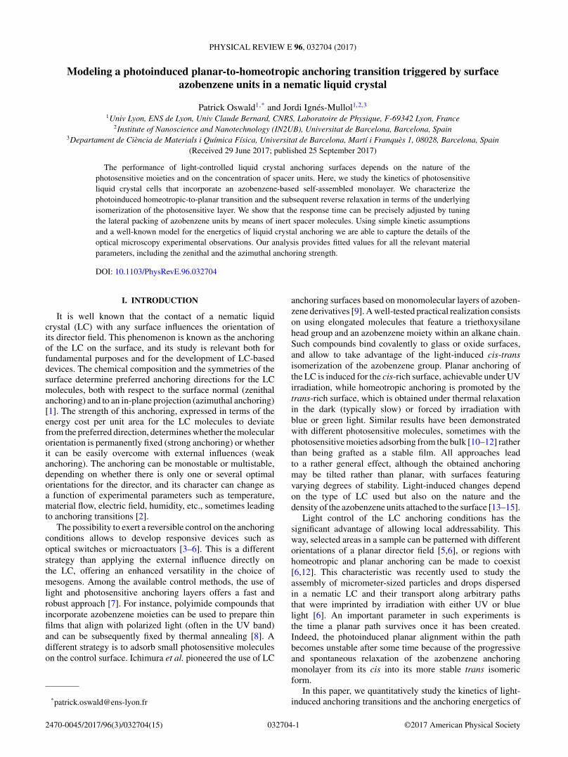
Second, we measured the plateau duration. It is important tonote here that this quantity is independent of the UV exposuretime tUV provided the latter is large enough. This is visiblein Fig. 3 measured with the same sample as in Fig. 1(b) atδT = −0.3 ◦C. This curve shows that, for tUV < 7s, thereis no plateau. On the other hand, a plateau develops whentUV > 7 s as we can see in Fig. 1(b) where the dashed line curvecorresponds to tUV = 22 s. In this regime, the plateau duration(denoted by tp1 in the following) increases monotonically from0 to a constant value as a function of tUV. The fact that theplateau duration tends to a constant at large tUV means thatthe concentration of cis-isomer saturates on the surfaces whentUV is long enough. This is the saturation regime in whichour subsequent experiments were performed. We found thattp1 strongly depends on CES as shown in Fig. 4. In this figure,each point represents an average over two to five measurementsrealized with different samples (about 40 in total). The typicalerror for each point is about ±20%. This graph shows thattp1 is an increasing function of the CES that diverges for acritical concentration close to 0.84. Above this concentration,the anchoring is no longer homeotropic at equilibrium butconical, until it becomes planar for CES = 1. Note that the
032704-3
PATRICK OSWALD AND JORDI IGNÉS-MULLOL PHYSICAL REVIEW E 96, 032704 (2017)
1600
1400
1200
1000
800
600
400
200
0
plat
eau
dura
tion
(s)
20015010050tUV (s)
tp1
FIG. 3. Plateau duration (tp1) as a function of the UV exposuretime. d = 21.63 μm, CES = 0.817, and δT = −0.3 ◦C.
critical concentration slightly depends on temperature. Thisis visible in Fig. 1(c) corresponding to CES = 0.847. For thisconcentration, the transmittance curve tends to 0 at long time atδT = −0.3, −2, and −5 ◦C, but to a finite value close to 0.15at δT = −10 ◦C, which corresponds to a director tilt angleθ ≈ 22◦. This means that for this sample, the equilibriumanchoring is no longer homeotropic at low temperature butconical.
Third, we measured at which time tp2 the homeotropic stateis recovered. This time is more difficult to measure than tp1
because of a frequent artifact which is visible in Fig. 1(c). Onthis example, a kind of shoulder (indicated by an arrow) is
clearly visible on the curve measured at δT = −0.3 ◦C, but itis not observed on the analogous curves shown in Figs. 1(a)and 1(b). This shoulder is due to the fact that, in this sample, thetime at which the anchoring ceases to be planar is not exactlythe same on the two plates. This was difficult to avoid in spiteof the two plates being always prepared simultaneously in thesame silane solution. The presence of this shoulder leads toan overestimation of tp2. This is the reason why we did notmeasure tp2 in the samples in which such artifact was clearlyvisible. Another difficulty was that the transmittance curve wasusually rounded at the end. For this reason, we measured tp2
as the time at which the transmittance decreases below 0.05.Measurements of tp2 are shown in Fig. 4.
To complete these measurements, we studied the aging ofthe photosensitive surface treatment. We found that, in general,the length of the plateau regularly decreases during the weeksthat follow the sample preparation. On the other hand, theshape of the transmittance curves remained unchanged as canbe seen in Fig. 5. In this figure, two sets of curves are shown:the solid curves were measured in a fresh sample and thedashed curves were measured in the same sample two monthslater. An important point to emphasize is that the decrease ofthe plateau duration tp1 depends on temperature. For instance,in Fig. 5, tp1 decreases by ∼150 s at δT = −0.3 ◦C, ∼190s at δT = −2 ◦C, ∼290 s at δT = −5 ◦C, and ∼460 s atδT = −10 ◦C. This observation will be discussed in the nextsection.
B. Model
To model the reported behavior, we propose that theanchoring potential on the surfaces results from a competition
tp1,
tp2
(103
s)
tp1,
tp2
(103
s)
tp1,
tp2
(103
s)
tp1,
tp2
(103
s)
CES
CES
CES
CES
4
3
2
1
0
0.80.60.40.20.0
5
4
3
2
1
0
0.80.60.40.20.0
8
6
4
2
0
0.80.60.40.20.0
8
6
4
2
0
0.80.60.40.20.0
)b()a(
(d)(c)
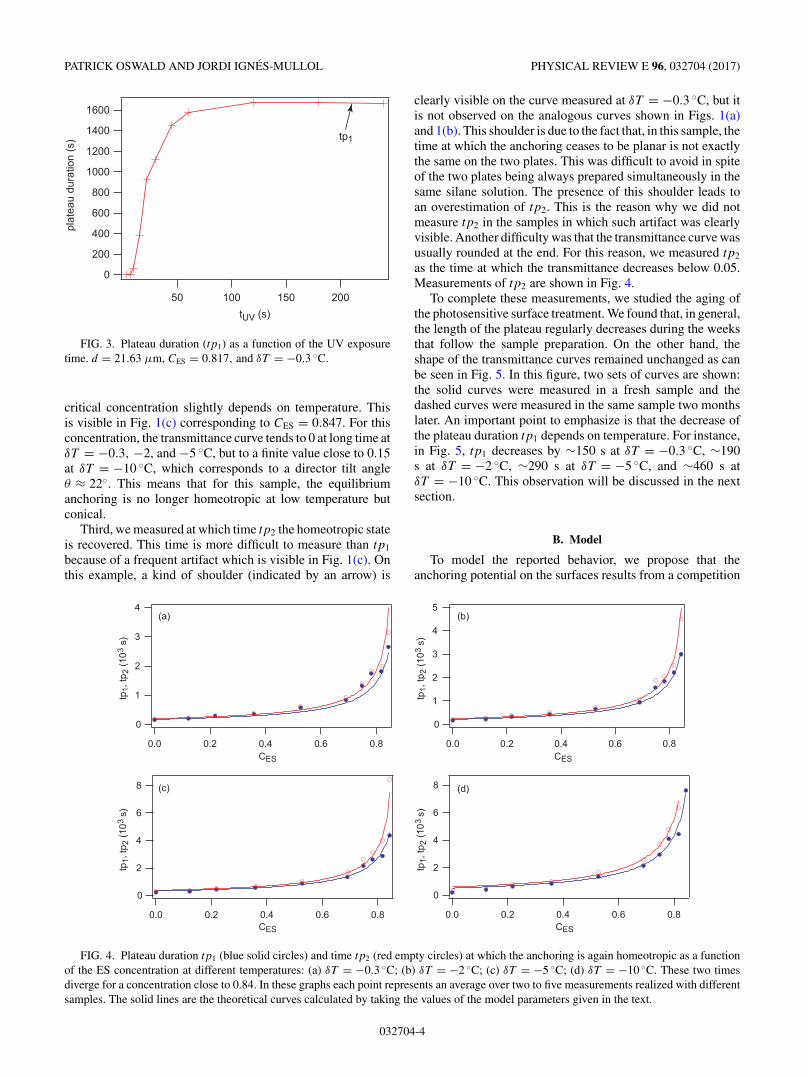
FIG. 4. Plateau duration tp1 (blue solid circles) and time tp2 (red empty circles) at which the anchoring is again homeotropic as a functionof the ES concentration at different temperatures: (a) δT = −0.3 ◦C; (b) δT = −2 ◦C; (c) δT = −5 ◦C; (d) δT = −10 ◦C. These two timesdiverge for a concentration close to 0.84. In these graphs each point represents an average over two to five measurements realized with differentsamples. The solid lines are the theoretical curves calculated by taking the values of the model parameters given in the text.
032704-4
MODELING A PHOTOINDUCED PLANAR-TO-HOMEOTROPIC . . . PHYSICAL REVIEW E 96, 032704 (2017)
0.8
0.6
0.4
0.2
0.0
32.521.510.50time (103 s)
trans
mitt
ance
-0.3°C
-2°C
-5°C
-10°C
FIG. 5. Transmittance curves measured with a fresh sample(solid lines) and with the same sample stored two months at roomtemperature (dashed lines). Except for the plateau duration, the curvesare essentially the same. d = 21.69 μm and CES = 0.69.
between the three kinds of molecules that occupy the surface:the ES molecules and the AS molecules in their cis and transconfigurations, respectively. Let x (respectively, 1 − x) be theconcentration of ES (respectively, AS) molecules attachedto the surface. If the surface attachment probability is thesame for both types of silane molecules, the bulk and surfacecompositions must be the same: x = CES. We make thisassumption in the following, knowing that this result wasshown by Noonan et al. [16] for self-assembled monolayerspepared with a mixture of alkyl-silanes of different chainlengths.
Each type of molecule is characterized by its own anchoringpotential W . As recalled in Ref. [20] the symmetry of thesurface (revolution) and of the nematic (inversion) imposes thatW (θ ) = W (−θ ) = W (π ± θ ) provided that there is no surfacepolarization, which we assume. In this case, the most generalform of W (θ ) is a Fourier expansion in cos(2nθ ) with n =1,2, . . .. In the following, we will only keep the first two termsin cos(2θ ) and cos(4θ ). We have seen that the ES moleculesgive a planar anchoring. For this reason, we write
WES = Wa
[1
2cos(2θ ) + βES
4cos(4θ )
](4)
with the anchoring energy Wa > 0 and |βES| < 1/2.For the the AS molecules, we must distinguish the two
isomers. For the trans-isomer which gives a homeotropicanchoring, we take
Wtrans = Wa
[−αtrans
2cos(2θ ) + βtrans
4cos(4θ )
], (5)
with αtrans > 0 and |βtrans| < αtrans/2 and for the cis-isomer,we take
Wcis = Wa
[αcis
2cos(2θ ) + βcis
4cos(4θ )
], (6)
with αcis > 0 and |βcis| < αcis/2, knowing that this isomerfavors a planar anchoring.
The next step is to calculate the resulting surface potential.Because of the nematic elasticity, the director field cannotdistort at the scale of a few molecular lengths. For this reasonθ is homogeneous on the surface and we assume that theglobal surface potential is simply a weighted average of theindividual potentials:
where y(t) is the fraction of cis-isomer in the layer at time t
by choosing t = 0 at the end of the UV exposure.Let us now calculate y(t). The most simple assumption is
to assume that the isomerization process follows a first-orderkinetics:
dy
dt= kI (1 − y) − γy, (8)
where I is the intensity of the UV light, which is keptconstant in our experiments, k is the trans-to-cis constant ofisomerization, and γ is the rate of spontaneous transformationof the cis-isomer into the more stable trans-isomer. In thisequation, the first term in the right-hand side describes thecreation of the cis isomer under UV and the second termdescribes its spontaneous destruction into the more stabletrans configuration. This equation shows that under constantUV illumination, the system reaches a stationary state with aconcentration of cis isomer given by
ysat = kI
kI + γ. (9)
In practice, we are in the saturation regime after the UVillumination. This means that at time t = 0, y = ysat. SolvingEq. 8 with this initial condition and I = 0 gives
y(t) = ysat exp
(− t
τ
), (10)
where τ = 1/γ is the cis-to-trans spontaneous relaxation time.As we will see later, the typical creation time under UV of thecis-isomer τUV = 1/(kI ) is much smaller than τ , for the usedUV light intensity. For this reason, we will take ysat = 1 in thefollowing.
We can now calculate the global surface potential. Substi-tution of WES, Wtrans, and Wcis by their expressions in Eq. (6)gives
The azimuthal angle θ (t) is finally given by minimizing W (θ,t)at each time.
Next, we show that this model predicts a continuous planar-to-homeotropic transition. The anchoring ceases to be planarwhen the concentration of cis isomer has decreased down toy1 given by α(y1) = 2β(y1) [20], which yields
y1 = (αtrans + 2βtrans)(1 − x) − (1 − 2βES)x
(1 − x)(αtrans + 2βtrans + αcis − 2βcis). (14)
032704-5
PATRICK OSWALD AND JORDI IGNÉS-MULLOL PHYSICAL REVIEW E 96, 032704 (2017)
This happens at a time tp1 that satisfies
tp1 = −τ ln(y1). (15)
Similarly, the anchoring is again homeotropic when theconcentration of cis isomer satisfies α(y2) = −2β(y2) [20],which gives
y2 = (αtrans − 2βtrans)(1 − x) − (1 + 2βES)x
(1 − x)(αtrans − 2βtrans + αcis + 2βcis). (16)
This occurs at a time tp2 given by
tp2 = −τ ln(y2). (17)
Note that, in agreement with experiments, tp1 divergeswhen y1 = 0 at the concentration
x1 = αtrans + 2βtrans
1 − 2βES + αtrans + 2βtrans, (18)
while tp2 diverges when y2 = 0 at the concentration
x2 = αtrans − 2βtrans
1 + 2βES + αtrans − 2βtrans. (19)
We observe x2 < x1 (Fig. 4), which imposes βtrans +αtransβES > 0. We emphasize that the anchoring at equilibrium(when I = 0) is homeotropic when x < x2, tilted when x2 <
x < x1 and planar when x > x1.This model can also be used to relate the plateau duration
tplateau as a function of the UV exposure time tUV in theunsaturated regime (Fig. 3). It is important to stress that,after relaxation following UV irradiation, the sample goesback to being homeotropic when y < y2. Although y2 > 0,no changes are detectable during the subsequent relaxationtowards the pure trans form of the AS layers. For this reason,we must follow a strict protocol for sample preparation duringexperimental repetitions. In practice, the curve of Fig. 3 wasobtained by first measuring tp2 for a long UV exposure time (inthe saturation regime). Once the sample was homeotropic, wewaited an additional time tw of the order of 30 min beforestarting a new measurement with the same sample and asmaller tUV. This protocol ensured that the value of y at thebeginning of each run (when we started the UV illumination)was always the same, namely,
y0 = y2 exp
(−tw
τ
). (20)
The above procedure was iterated using smaller values of tUV
until no plateau was observed during relaxation.The next step consists on calculating from the kinetic Eq. (8)
the value y0 of y at the end of each UV illumination. Solvingthis equation with I �= 0 is straightforward and gives, byassuming that τUV � τ (an assumption that we will checka posteriori),
y0 = 1 − (1 − y0) exp
(− tUV
τUV
). (21)
Finally, the plateau duration is given by
tplateau = τ ln
(y0
y1
)= τ ln
[1 − (1 − y2e
− twτ )e− tUV
τUV
y1
]. (22)
This formula shows that tplateau = 0 when tUV is smaller than
tminUV = τUV ln
[1 − y2e
− twτ
1 − y1
], (23)
which can be estimated from the data in Fig. 3 as tminUV ≈ 7s.
Finally, this model can be used to understand the observedeffect of sample aging. The simplest assumption is to supposethat, as the sample ages, a fraction 1 − y0 of the azosilanemolecules loses its photosensibility. In other words, thefraction y of cis-isomer after UV illumination is y0 < 1. Underthese conditions, the problem remains the same, just replacingEq. (10) with
y(t) = y0 exp
(− t
τ
). (24)
A direct consequence is that the transmittance curves remainunchanged, except that the time axis is shifted by −τ ln(y0).This agrees well with experiments shown in Fig. 5.
C. Analysis of the experimental data
We next proceeded to test this model with our experimentaldata. The unknown parameters are the characteristic time τ
and the five dimensionless parameter αtrans, αcis, βtrans, βcis,and βES. Note that Wa does not play any role here becausethe director field is not distorted in the sample during therelaxation process. In practice all these parameters dependon temperature, which gives 6 free parameters for eachtemperature, i.e., 24 fit parameters for the 4 temperaturesstudied.
It is nonetheless possible to immediately reduce this numberby noticing that during the sample aging the decrease of theplateau duration tp1 is proportional to τ with a proportionalitycoefficient −ln (y0) independent of temperature. This allowedus to directly determine the temperature dependence of τ bymeasuring the time shift of the curves as a function of tem-perature. By setting τ ≡ τ (−0.3 ◦C), we found that in averageτ (−2 ◦C) ≈ 1.25τ , τ (−5 ◦C) ≈ 1.88τ , and τ (−10 ◦C) ≈ 3τ .This reduces to 21 the number of fit parameters.
We proceeded by simultaneously fitting the eightexperimental curves of Fig. 4 with Eqs. (14) to (17) by usingthe Global Fit package of Igor Pro (WaveMetrics Inc.). Ourfit parameters were wt1 = αtrans + 2βtrans, wc1 = αcis − 2βcis,wt2 = αtrans − 2βtrans, wc2 = αcis + 2βcis, βES, and τ . This fitwas performed by imposing to each parameter wt1, wc1, wt2,wc2, and βES to be the same for the two curves tp1(x) andtp2(x) measured at each temperature. With these constraints,we found that the global fit converged by giving τ =1465 ± 161 s and values for the other parameters essentiallyindependent of temperature—but with large errors. This isdue to the too large number of fit parameters with respect tothe number of experimental points (about 250 by taking theraw data and not the average values shown for more clarity inFig. 4). For this reason, we redid our fit by imposing that theparameters wt1 and wc1, wt2, wc2, and βES were independentof temperature, as the first fit suggested. Under these new con-straints, the number of independent fit parameters was reducedto 6, which was much more reasonable. The values of thefit parameters obtained in this way are τ = 1387 ± 82 s,
032704-6
MODELING A PHOTOINDUCED PLANAR-TO-HOMEOTROPIC . . . PHYSICAL REVIEW E 96, 032704 (2017)
This fit shows that βcis and βES are very close to 0. Thismeans that WES and Wcis are well described by a potentialof Rapini-Papoular type, proportional to cos(2θ ). Thecorresponding theoretical curves are shown as solid lines inFig. 4. As we can see, the fit is satisfactory.
With these fitted parameters, we proceeded to calculate thetransmittance curves that correspond to the samples in Fig. 1.The calculations were performed with Mathematica by usingEqs. (2) and (3) and the values of the birefringence given inFig. 2. In this calculation, angle θ (t) was numerically calcu-lated by minimizing W (θ ) at each time. The correspondingtheoretical curves are shown in Fig. 6 and compare well withthe experimental ones shown in Fig. 1.
Furthermore, we can reproduce the curve of Fig. 3 showingtplateau versus tUV. In this example, x = 0.817 and δT =−0.3 ◦C. From Eqs. (14) and (16), we calculated, using thevalues of the α and β coefficients given above, y1 = 0.29and y2 = 0.192. At this temperature, τ = τ = 1387 s. Exper-imentally, tw ≈ 1800 s and tmin
UV ≈ 7 s, which gives, by usingEq. (23), τUV ≈ 24 s. We see here that τUV � τ , consistentlywith the assumption above that led to the derivation of Eq. (21).From these values, tplateau can be calculated as a function of tUV
using Eq. (22). The corresponding theoretical curve, shown inFig. 7, is again in correct agreement with the experimental data(Fig. 3).
Using the above fitted parameters, we estimated the valueof y0 for the aged sample shown in Fig. 5. For the two curvesmeasured at δT = −0.3 ◦C, the shift is of about 150 s, whichmeans that −τ ln(y0) = 150 s. This gives y0 = 0.9 by takingτ = 1387 s. This means that 10% of the azosilane moleculeshave lost their efficiency after two months.
Finally, we can explore the anchoring potential landscapeduring the planar to homeotropic transition by computingthe time evolution of the anchoring potential. In Fig. 8, weplot W [θ (t)] for δT = −5 ◦C and x = 0.817 [same sampleas in Figs. 1(b) and 6(b)]. This figure clearly shows thecontinuous passage between the planar and homeotropicanchoring. Another interesting point is that the potential is veryflat in the transition region. This can result in the coexistenceof regions with slightly different anchoring angle, which mayexplain why we often observe under the microscope smallspatial inhomogeneities in the transmitted intensity duringthe transition. These local intensity variations lead to theexperimental transmittance curves shown in Fig. 1 to usuallypass through a maximum that is slightly smaller than 1(contrary to the theoretical curves shown in Fig. 6).
D. Independent measurement of the relaxation time andvalidation of the model
To validate the assumptions made in the model abovebased on the observed evolution of LC anchoring during theisomerization of the AS layer, we performed UV-VIS spec-
0.2 0.4 0.6 0.8
0.2
0.4
0.6
0.8
1.0
time (103 s)
trans
mitt
ance
2 4 6 8
0.2
0.4
0.6
0.8
1.0
time (103 s)
trans
mitt
ance
time (103 s)
trans
mitt
ance
0.00
0.00
0.00 5 10 15 20 25
0.2
0.4
0.6
0.8
1.0
-0.3°C
-2°C
-5°C
-10°C
-0.3°C
-2°C
-5°C
-10°C
(a)
(b)
(c)-0.3°C
-2°C
-5°C
-10°C
FIG. 6. Theoretical transmittance curves calculated from themodel for the samples of Fig. 1 by taking τ = 1387 s and the valuesof the parameters α and β given in the text.
trophotometry measurements. We used a Shimadzu 1700 spec-trophotometer equipped with a thermostatic cuvette holder,connected to a Julabo MB-12 water circulation thermostat.We built a custom adapter to study flat LC cells instead of thestandard volumetric cuvettes. This double-beam instrumentfeatures a reference beam, where we placed a homeotropicLC cell. The custom holders featured identical 6 mm circular
032704-7
PATRICK OSWALD AND JORDI IGNÉS-MULLOL PHYSICAL REVIEW E 96, 032704 (2017)
0 50 100 150 200
250
500
750
1000
1250
1500
1750
t plat
eau (s
)
tUV (s)
FIG. 7. Theoretical plateau duration as a function of the UVillumination time. The curve has been calculated for the same sampleas in Fig. 3 and in the same experimental conditions.
windows to restrict the region of observation. Both the sampleand reference cells had a gap d = 21.5 μm.
(a)
(b)
W (θ
) / W
aW
(θ) /
Wa
θ (rad)
θ (rad)
1
2
3
4
56
1
2
3
4
5
0 0.25 0.5 0.75 1 1.25 1.5
-0.02
0
0.02
0.04
0 0.25 0.5 0.75 1 1.25 1.5
-0.4
-0.2
0
0.2
0.4
6
FIG. 8. Time evolution of the theoretical anchoring potentialwhen x = 0.817 [as in Figs. 1(b) and 4(b)] and δT = −5 ◦C. Graph(a) shows the global evolution of the potential. The curves 1 to 6 havebeen calculated at time t = 0 s, 1000 s, 2000 s, 3500 s, 6000 s, and ∞,respectively. Graph (b) shows the potential during the transition fromplanar to homeotropic. Curves 1 to 6 have been calculated at timet = 3150 s, 3350 s, 3550 s, 3750 s, 4050 s, and 4450 s, respectively.In this example, tp1 ≈ 3200 s and tp2 ≈ 4300 s.
1.0
0.8
0.6
0.4
0.2
0.0
norm
aliz
ed a
bsor
banc
e
1086420
time (103s)
FIG. 9. Normalized absorbance of a CES = 0.69 sample at δT =−5 ◦C after 120 s irradiation with UV light. The feature pointed toby an arrow corresponds to the planar-to-homeotropic transition. Thesolid line corresponds to a fit to first order kinetics.
We took advantage of the distinctive absorption bandof the trans isomer of our azosilane compound, with apeak at λ = 350 nm. At this wavelength, the cis isomerhas a negligible absorbance. As a consequence, we couldmonitor the isomerization kinetics by using Lambert-Beers’equation, Abs350 nm ∝ CAS(trans). Although we lacked an abso-lute calibration to directly convert absorbance data into ASconcentration, a comparison between different well-definedregions yielded useful information. All the samples used inthese measurements were prepared using fused-silica plates tooptimize the signal-to-noise ratio in the UV. We verified thatthe protocol described above for the functionalization of glassplates yielded analogous effects when applied to fused silica.
In a typical experiment, the sample was allowed to relaxin the dark at the target temperature. For best results, sampleswere kept overnight inside the spectrophotometer, avoidingany contact with visible or UV light. This ensured thatthe initial condition corresponded to 100% trans AS. Afterensuring that the absorbance reading at 350 nm was stable,we irradiated the sample with the same UV LED lightsource described above. Because of the configuration of theinstrument, we needed to use a 45◦ metallic mirror to irradiatethe sample that was held in the thermostatic holder. Afterthe target irradiation time, the absorbance was monitored forseveral hours, until the exponential relaxation had approachedthe high absorbance plateau, allowing to fit the relaxation tothe first-order kinetics expressed in absorbances,
A = A∞ + (A0 − A∞)e−t/τ . (25)
In Fig. 9 we show a typical experiment using a sample withCES = 0.69, where irradiation with UV light was performedfor 120 s to ensure that the AS was nearly 100% in the cisisomer. About 1500 s after relaxation began, we observeda shift in the absorbance curve (indicated by an arrow).By comparing with the tp1 values measured above (Fig. 4)we concluded that this feature corresponded to the planar-to-homeotropic transition, which results in a change in thesample transmittance due to the birefringence of CCN37. Theduration of the transition observed here is consistent with
032704-8
MODELING A PHOTOINDUCED PLANAR-TO-HOMEOTROPIC . . . PHYSICAL REVIEW E 96, 032704 (2017)
tp2 − tp1 for the same experimental conditions in Fig. 4.Since our reference cell was homeotropic, we only usedabsorbance data well after this transition was completed toobtain the relaxation time. For the data in Fig. 9, our fit yieldsτ = 2711 ± 25 s. This value is consistent to the one obtainedin Sec. III C, namely, τ (−5 ◦C) ∼ 1.88τ = 2607 ± 154 s.Similar measurements were performed for a wide temperaturerange, confirming the good agreement between values forthe cis-to-trans relaxation time estimated from absorbancemeasurements and from the fit to the transmittance data(Fig. 10). On top of that, this result validates our assumptionson the aging of the photosensitive monolayers from which wededuced the temperature dependence τ (T )/τ .
The absorbance data in Fig. 9 can be used to estimatethe monolayer composition required to have homeotropicanchoring. If, after the 120 s irradiation, all AS moleculesare in the cis form (consistently with the assumption in themodel), and, when the plateau is finally reached, all ASmolecules are in the trans form, we conclude, by comparingrelative absorbances, that for anchoring to be homeotropicwe need about 42% of the AS molecules to be in thetrans form. Considering that this sample contains about 31%AS molecules and 69% ES molecules (CES = 0.69), thenhomeotropic anchoring requires about 13% of the total silanemolecules in the monolayer to be AS trans. This is consistentwith the fact that tp1 diverges when more than 84% of thesilane molecules are ES (Fig. 5). In other words, the samplewill be planar (cannot be homeotropic) when more than 84%of the silane molecules are ES.
IV. ZENITHAL ANCHORING ENERGY
A. Estimation from wall analysis
From the previous transmittance measurements, it isimpossible to obtain the anchoring energy Wa . However,useful information about Wa can be obtained by examiningthe domain walls that form in the samples during the UVillumination. Indeed, two types of domain may developin the samples during the homeotropic-to-planar transition
FIG. 11. Ising walls and disinclination lines (indicated by thearrows) observed immediately after the UV illumination. d =21.69 μm and CES = 0.69 and δT = −0.3 ◦C.
because the director can indifferently rotate clockwise orcounterclockwise in the plane perpendicular to the magneticfield. As a result, π -walls must form between these domainsas shown in Fig. 11, in an image taken immediately afterthe UV illumination. Observation between crossed polarizersat 45◦ of the magnetic field shows that the intensity signalmeasured along a line perpendicular to the wall passes throughtwo minima (Fig. 12). This indicates that the director goes outof the plane perpendicular to the magnetic field. For this reason,the walls are Bloch walls [2]. This observation also explainsthe formation of the disclination lines (marked by an arrow inFig. 11) that form on the walls. These lines separate two wallportions in which the director rotates in opposite directions.The observation of Bloch walls (rather than Ising walls inwhich the director would rotate in the plane perpendicular to�B) clearly indicates that the director prefers to remain parallelto the surfaces rather than perpendicular to the magnetic field.This is the result of a competition between the anchoring andthe magnetic field.
To quantify this competition, we developed a very simplemodel for π -walls under a magnetic field. In this model, the
1.0
0.8
0.6
0.4
0.2
0.0
150100500-50-100
-0.3°C
-2°C
-5°C
-10°C
trans
mitt
ance
position (μm)
FIG. 12. Typical intensity profiles measured at different δT
between crossed polarizers along a line perpendicular to the walland perpendicular to the magnetic field (line ab in Fig. 11). Samplethickness d = 21.69 μm and CES = 0.69.
032704-9
PATRICK OSWALD AND JORDI IGNÉS-MULLOL PHYSICAL REVIEW E 96, 032704 (2017)
xy
z
B
+d/2
−d/2
n(+∞) →
→Wall
Ising
Bloch
n(y)→
x
y
z
N
n(−∞) →
→n(+∞) n(−∞) →
(a)
(b)
FIG. 13. (a) Coordinate system for a π -wall in a magnetic field;(b) Representation on the unit sphere S2 of the director field across aBloch wall (blue trajectories) and an Ising wall (red trajectories). Foreach type of walls, there are two possible trajectories (drawn in solidand dashed lines, respectively) depending on the sense of rotation ofthe director.
director �n has for components nx , ny , and nz = (1 − n2x −
n2y)1/2. The z axis is taken perpendicular to the surfaces,
the magnetic field �B is parallel to the x axis, and the wallis perpendicular to the y axis [Fig. 13(a)]. We need tominimize the total energy including the elastic, magnetic, andanchoring energies with nx(y,z) and ny(y,z) and the boundaryconditions:
ny(+∞,z) = 1, nx(+∞,z) = nz(+∞,z) = 0,
ny(−∞,z) = −1, nx(+∞,z) = nz(+∞,z) = 0. (26)
This is a very difficult task which cannot be performedanalytically, even in isotropic elasticity. For this reason andto determine for which typical value of the anchoring energyones passes from an Ising to a Bloch wall, we assume that nx
and ny do not depend on z and we propose as an ansatz that
nx(y) = C
cosh(
y
ξ
) ,
ny(y) = tanh
(y
ξ
), (27)
where 4ξ is the typical wall thickness. This director fieldsatisfies the boundary conditions Eq. (26) and describes anIsing wall when C = 0 and a Bloch wall when C = 1. In thefirst case, the director describes one of the two red trajectoriespassing though the poles on the unit sphere [Fig. 13(b)]. Inthe second case, the director describes on the unit sphere one
of the two blue trajectories on the equator [Fig. 13(b)]. In theother cases (0 < C < 1), the director rotates in an intermediateplane.
To calculate in which limit a Bloch wall is observed, wecalculated the total energy of the wall. Assuming K = K1 =K3 (the wall is here of splay-bend type) the Frank and magneticenergies reduce to
fv
K= 1
2
(n2
x,z + n2y,y + n2
z,y
) + 1
2
n2x
ξ 2m
, (28)
where ξm =√
μ0K
−χa
1B
is the magnetic coherence length, μ0 is
the vacuum permeability, and χa is the (negative) magneticanisotropy. For the surface energy, we chose a simplified formthat neglects the cos(4θ )-term (this is justified as β � α forES and AS). In this case, the surface energy (which we takeequal to 0 at infinity in the y direction) reads at time t = 0:
fs
K= α(0)
2la[cos(2θ ) + 1] = α
la[1−nx(y)2−ny(y)2], (29)
where la = KWa
is the anchoring extrapolation length and α ≡α(0) = CES + αcis(1 − CES).
The next step is to calculate the wall energy F . A straight-forward integration of fv and fs over y and z coordinatesyields (per unit length along x)
F
K= d
ξ+ ξ
(4α
la− 4
αC2
la+ C2d
ξ 2m
). (30)
Minimization as a function of ξ gives
ξ−1 =√
4α(1 − C2)
lad+ C2
ξ 2m
(31)
and
F
K=
√4α
la+ C2
(d
ξ 2m
− 4α
la
). (32)
From these formulas we deduce that if la >4αξ 2
m
dthe wall is
of the Ising type (C = 0), of width 4ξ = 2√
lad/α, whereas if
la <4αξ 2
m
da Bloch wall of width 4ξ = 4ξm must be observed
(C = 1). Experimentally, we are clearly in the second case,which means that
la = K
Wa
<4αξ 2
m
d. (33)
In CCN-37, ξm ∼ 5 μm by taking B = 1 T and the valuesof χa and K (with K ≈ K1+K3
2 ) given in Ref. [18]. As aconsequence this very simple model predicts a wall thick-ness of the order of 4ξm ≈ 20 μm, which agrees with theintensity profiles measured experimentally (see Fig. 12) andan extrapolation length K/Wa < 5 μm (knowing that for thesample shown in Fig. 11, α ≈ 1). In practice, la could bededuced by numerically calculating the director field and thecorresponding transmittance profiles and by then comparingthe theoretical profiles with the experimental ones. However,these calculations are complicated and may not be precise ifthe anchoring length is too small. For this reason, we preferredusing another more simple method.
032704-10
MODELING A PHOTOINDUCED PLANAR-TO-HOMEOTROPIC . . . PHYSICAL REVIEW E 96, 032704 (2017)
0.00
time (103 s)
-0.3°C
-2°C
-5°C-10°C
0.2 0.4 0.6 0.8 1
0.2
0.4
0.6
0.8
1.0
0.8
0.6
0.4
0.2
0.0
10.80.60.40.20time (103 s)
trans
mitt
ance
trans
mitt
ance
1.0
-0.3°C
-2°C
-5°C-10°C
(a)
(b)
0.75 μm0.50 μm0.25 μm0.10 μm
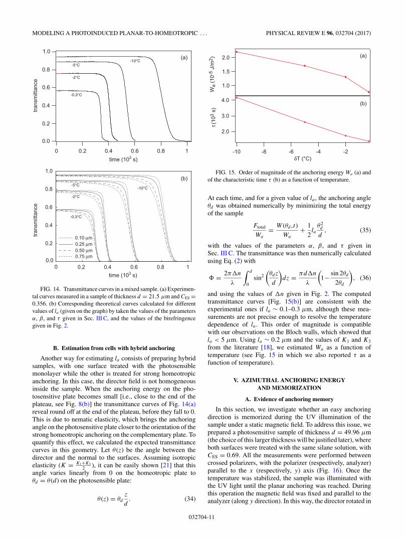
FIG. 14. Transmittance curves in a mixed sample. (a) Experimen-tal curves measured in a sample of thickness d = 21.5 μm and CES =0.356. (b) Corresponding theoretical curves calculated for differentvalues of la (given on the graph) by taken the values of the parametersα, β, and τ given in Sec. III C, and the values of the birefringencegiven in Fig. 2.
B. Estimation from cells with hybrid anchoring
Another way for estimating la consists of preparing hybridsamples, with one surface treated with the photosensiblemonolayer while the other is treated for strong homeotropicanchoring. In this case, the director field is not homogeneousinside the sample. When the anchoring energy on the pho-tosensitive plate becomes small [i.e., close to the end of theplateau, see Fig. 8(b)] the transmittance curves of Fig. 14(a)reveal round off at the end of the plateau, before they fall to 0.This is due to nematic elasticity, which brings the anchoringangle on the photosensitive plate closer to the orientation of thestrong homeotropic anchoring on the complementary plate. Toquantify this effect, we calculated the expected transmittancecurves in this geometry. Let θ (z) be the angle between thedirector and the normal to the surfaces. Assuming isotropicelasticity (K = K1+K3
2 ), it can be easily shown [21] that thisangle varies linearly from 0 on the homeotropic plate toθd = θ (d) on the photosensible plate:
θ (z) = θd
z
d. (34)
Wa
(10-
5 J/
m2 )
4.0
3.0
2.0
τ (10
3 s)
-10 -8 -6 -4 -2δT (°C)
1.0
1.5
2.0 (a)
(b)
FIG. 15. Order of magnitude of the anchoring energy Wa (a) andof the characteristic time τ (b) as a function of temperature.
At each time, and for a given value of la , the anchoring angleθd was obtained numerically by minimizing the total energyof the sample
Ftotal
Wa
= W (θd,t)
Wa
+ 1
2la
θ2d
d, (35)
with the values of the parameters α, β, and τ given inSec. III C. The transmittance was then numerically calculatedusing Eq. (2) with
� = 2π�n
λ
∫ d
0sin2
(θdz
d
)dz = πd�n
λ
(1− sin 2θd
2θd
), (36)
and using the values of �n given in Fig. 2. The computedtransmittance curves [Fig. 15(b)] are consistent with theexperimental ones if la ∼ 0.1–0.3 μm, although these mea-surements are not precise enough to resolve the temperaturedependence of la . This order of magnitude is compatiblewith our observations on the Bloch walls, which showed thatla < 5 μm. Using la ∼ 0.2 μm and the values of K1 and K3
from the literature [18], we estimated Wa as a function oftemperature (see Fig. 15 in which we also reported τ as afunction of temperature).
V. AZIMUTHAL ANCHORING ENERGYAND MEMORIZATION
A. Evidence of anchoring memory
In this section, we investigate whether an easy anchoringdirection is memorized during the UV illumination of thesample under a static magnetic field. To address this issue, weprepared a photosensitive sample of thickness d = 49.96 μm(the choice of this larger thickness will be justified later), whereboth surfaces were treated with the same silane solution, withCES = 0.69. All the measurements were performed betweencrossed polarizers, with the polarizer (respectively, analyzer)parallel to the x (respectively, y) axis (Fig. 16). Once thetemperature was stabilized, the sample was illuminated withthe UV light until the planar anchoring was reached. Duringthis operation the magnetic field was fixed and parallel to theanalyzer (along y direction). In this way, the director rotated in
032704-11
PATRICK OSWALD AND JORDI IGNÉS-MULLOL PHYSICAL REVIEW E 96, 032704 (2017)
P
A
x
y
n(z)B →→
φ
α = ωt
(z)
Easy axis
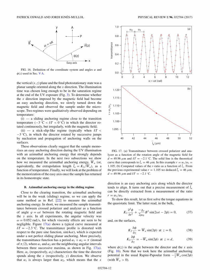
FIG. 16. Definition of the coordinate system and angles α andφ(z) used in Sec. V A.
the vertical (x,z) plane and the final photostationary state was aplanar sample oriented along the x direction. The illuminationtime was chosen long enough to be in the saturation regimeat the end of the UV exposure (Fig. 3). To determine whetherthe x direction imposed by the magnetic field had becomean easy anchoring direction, we slowly turned down themagnetic field and observed the sample under the micro-scope. Two regimes were qualitatively observed depending ontemperature:
(i) — a sliding anchoring regime close to the transitiontemperature (−3 ◦C < δT < 0 ◦C) in which the director ro-tated continuously, but irregularly, with the magnetic field;
(ii) — a stick-slip-like regime (typically when δT <
−3 ◦C), in which the director rotated by successive jumpsby nucleation and propagation of anchoring walls on thesurfaces.
These observations clearly suggest that the sample memo-rizes an easy anchoring direction during the UV illuminationwith an azimuthal anchoring energy that strongly dependson the temperature. In the next two subsections we showhow we measured the azimuthal anchoring energy, Wa (or,equivalently, the extrapolation length la = K2/Wa), as afunction of temperature. Finally, we will look at the problem ofthe memorization of the easy axis once the sample has returnedin its homeotropic state.
B. Azimuthal anchoring energy in the sliding regime
Close to the clearing transition, the azimuthal anchoringwill be in the weak (sliding) regime, so we can apply thesame method as in Ref. [22] to measure the azimuthalanchoring energy. In short, we measured the sample transmit-tance between crossed polarizer and analyzer as a functionof angle ϕ = ωt between the rotating magnetic field andthe y axis. In all experiments, the angular velocity wasω = 0.052 rad/s, for which viscosity effects are seen to benegligible. Figure 17(a) shows a typical curve measured atδT = −2.3 ◦C. The transmittance profile is distorted withrespect to the pure sine function, sin(4ωt), which is expectedunder a not perfect sliding planar anchoring. More precisely,the transmittance function has a period α1 + α2 = π (insteadof π/2), where α1 and α2 are the neighboring angular intervalsbetween three successive maxima, as shown in Fig. 17(a).Here, α1 (respectively, α2) characterizes the time the directorspends along the x (respectively, y) direction. We observethat α1 is always larger than α2, which means that the x
1.0
0.8
0.6
0.4
0.2
0.0
tran
smit
tan
ce
121086420
α = ωt (rad)
(a)
(b)
α1α2
1.120
1.115
1.110
1.105
1.100
1.095
r = α
1/α
2
52504846444240
la ( μm)
FIG. 17. (a) Transmittance between crossed polarizer and ana-lyzer as a function of the rotation angle of the magnetic field ford = 49.96 μm and δT = −2.1 ◦C. The solid line is the theoreticalcurve that corresponds to la = 46 μm. In this example r = α1/α2 =1.105; (b) Computed values of the r-ratio as a function of la . Fromthe previous experimental value r = 1.105 we deduced la = 46 μm.d = 49.96 μm and δT = −2.1 ◦C.
direction is an easy anchoring axis along which the directortends to align. It turns out that a precise measurement of lacan be directly extracted from a measurement of the ratior = α1/α2.
To show this result, let us first solve the torque equations inthe quasistatic limit. The latter read, in the bulk,
K2∂2φ
∂t2+ −χa
2μ0B2 sin(2ωt − 2φ) = 0, (37)
and, on the surfaces,
K2∂φ
∂z= Wa sin(2φ) at z = 0, (38)
K2∂φ
∂z= −Wa sin(2φ) at z = d, (39)
where φ(z) is the angle between the director and the x axis(Fig. 16). Note that we took here the azimuthal anchoringpotential in the usual Rapini-Papoular form − 1
2Wa cos(2φ)(with Wa > 0).
032704-12
MODELING A PHOTOINDUCED PLANAR-TO-HOMEOTROPIC . . . PHYSICAL REVIEW E 96, 032704 (2017)
From the above equations, the director profile can beobtained analytically in the limit d � ξm (which is metexperimentally since d ≈ 50 μm and ξm ≈ 5 μm) [22]. Thesolution reads, by using the dimensionless variable Z = z/d:
φ(Z) = ωt + (φS − ωt)cosh
(Z−1/2d/ξm
)− 1
cosh(
12d/ξm
)− 1
, (40)
where φS is the angle on the surfaces given by the equation
ξm
lasin(2φS) + sin(φS − ωt) = 0. (41)
We calculated the transmittance curves that correspondsto the director profile given by Eq. (40) and to φS given byEq. (41) using Mathematica and the Jones matrix formalism.The sample thickness was discretized into 100 slabs, whichwas largely enough to ensure convergence. The numericalvalues of the material constants are given in the Appendix.The transmittance curves depend on la , which is unknownand can be fitted by comparing the computed curves with theexperimental ones [Fig. 17(a)]. In fact, the most remarkablefeature of the transmittance curves, namely, the asymmetrybetween α1 and α2 depends monotonically on la . In Fig. 17(b)we show the computed dependence of the ratio between thesetwo angles, r = α1/α2, as a function of la . By measuring r ina experimental realization and comparing with this calibrationcurve, we can extract the value for la . For instance, for the dataset in Fig. 17(a) we measured r =1.105, which correspondsto la = 46 μm in Fig. 17(b). The computed curve agrees verywell with the experimental one. This checking is importantbecause it confirms that the anchoring remains planar duringa complete revolution, an assumption that we made implicitlyfrom the beginning.
This method was systematically applied in the slidingregime, for temperatures close to the clearing transitiontemperature. The values of la obtained this way and the corre-sponding values of the anchoring energy Wa calculated withthe values of K2 given in the Appendix are shown in Fig. 18.This graph shows that la (Wa) strongly increases (decreases)but does not diverge (vanish) when the transition temperature isapproached. This means that even at the transition temperaturean easy anchoring direction is memorized.
C. Azimuthal anchoring energy far from the transition
The method used in the previous section to estimate labecomes imprecise when the latter is too small, typicallyless than 20 μm, and fails to apply if la < 2ξm ≈ 12 μm,since φS ceases to be a monotonically increasing functionof ωt and presents jumps for some values of ωt with anhysteretic behavior when the direction of rotation is reversed.In this regime, it is still possible to estimate Wa for magneticfield rotations smaller than π/4 by calculating the theoreticaltransmittance curves with the Jones matrix method and thedirector field profile obtained from the numerical solutionof Eqs. (37)–(39). The calculations were performed withMathematica by using an appropriate shooting method to solvethe differential equations and selecting the good solution,looking for the value of la that best fits the experimental
400
300
200
100
l a (
μm)
-5 -4 -3 -2 -1 0δT (°C)
2
4
6
0.01
2
4
6
0.1
2
4
6
Wa
(10-6
J/m
2 )
-5 -4 -3 -2 -1 0δT (°C)
(a)
(b)
FIG. 18. (a) Azimuthal extrapolation length as a function oftemperature. The points on the right of the vertical dashed line havebeen obtained with the rotating-field method. The points on the lefthave been measured with the static method. (b) Azimuthal anchoringenergy as a function of temperature. The solid lines are guides for theeye.
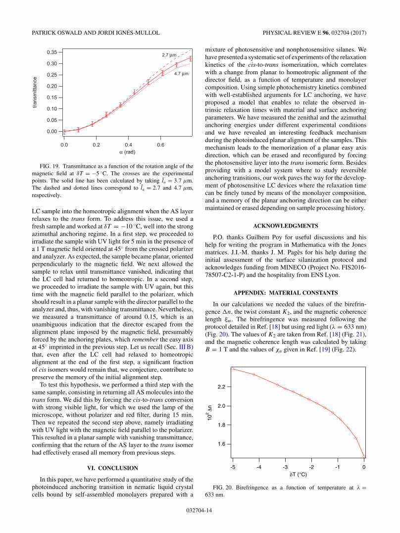
data. An example is shown in Fig. 19 for δT = −5 ◦C. Threetheoretical curves, calculated by taking the values of thematerial constants given in the Appendix, are compared tothe data. We observe that this method yields an estimatefor la with an accuracy better than 1 μm. The values of laobtained this way are combined in Fig. 18 with those in thesliding anchoring regime. By extrapolating this curve, one seesthat when δT < −6 ◦C, la � 1μm. Unfortunately, we werenot able to measure la in this regime of strong anchoring.We observe that Wa ∼ 10−6J m−2 as we enter this regime,consistently with estimates reported in the literature for ashorter chain azobenzene derivative [15].
D. About the memorization of the easy axis
A final question we address is whether the easy axismemorized in planar samples within the strong anchoringregime can be reset and reconfigured. As is the usual caseunder strong planar anchoring, the memory of an easy axis isnot lost even if the sample is cycled through the isotropic phase.In our case, however, we have an additional resource: we cantake advantage of the reversible isomerization that returns the
032704-13
PATRICK OSWALD AND JORDI IGNÉS-MULLOL PHYSICAL REVIEW E 96, 032704 (2017)
0.35
0.30
0.25
0.20
0.15
0.10
0.05
0.00
trans
mitt
ance
0.60.40.20.0α (rad)
4.7 μm
2.7 μm
FIG. 19. Transmittance as a function of the rotation angle of themagnetic field at δT = −5 ◦C. The crosses are the experimentalpoints. The solid line has been calculated by taking la = 3.7 μm.The dashed and dotted lines correspond to la = 2.7 and 4.7 μm,respectively.
LC sample into the homeotropic alignment when the AS layerrelaxes to the trans form. To address this issue, we used afresh sample and worked at δT = −10 ◦C, well into the strongazimuthal anchoring regime. In a first step, we proceeded toirradiate the sample with UV light for 5 min in the presence ofa 1 T magnetic field oriented at 45◦ from the crossed polarizerand analyzer. As expected, the sample became planar, orientedperpendicularly to the magnetic field. We next allowed thesample to relax until transmittance vanished, indicating thatthe LC cell had returned to homeotropic. In a second step,we proceeded to irradiate the sample with UV again, but thistime with the magnetic field parallel to the polarizer, whichshould result in a planar sample with the director parallel to theanalyzer and, thus, with vanishing transmittance. Nevertheless,we measured a transmittance of around 0.15, which is anunambiguous indication that the director escaped from thealignment plane imposed by the magnetic field, presumablyforced by the anchoring plates, which remember the easy axisat 45◦ imprinted in the previous step. Let us recall (Sec. III B)that, even after the LC cell had relaxed to homeotropicalignment at the end of the first step, a significant fractionof cis isomers would remain that, we conjecture, contribute topreserve the memory of the initial alignment step.
To test this hypothesis, we performed a third step with thesame sample, consisting in returning all AS molecules into thetrans form. We did this by forcing the cis-to-trans conversionwith strong visible light, for which we used the lamp of themicroscope, without polarizer and red filter, during 15 min.Then we repeated the second step above, namely irradiatingwith UV light with the magnetic field parallel to the polarizer.This resulted in a planar sample with vanishing transmittance,confirming that the return of the AS layer to the trans isomerhad effectively erased all memory from previous steps.
VI. CONCLUSION
In this paper, we have performed a quantitative study of thephotoinduced anchoring transition in nematic liquid crystalcells bound by self-assembled monolayers prepared with a
mixture of photosensitive and nonphotosensitive silanes. Wehave presented a systematic set of experiments of the relaxationkinetics of the cis-to-trans isomerization, which correlateswith a change from planar to homeotropic alignment of thedirector field, as a function of temperature and monolayercomposition. Using simple photochemistry kinetics combinedwith well-established arguments for LC anchoring, we haveproposed a model that enables to relate the observed in-trinsic relaxation times with material and surface anchoringparameters. We have measured the zenithal and the azimuthalanchoring energies under different experimental conditionsand we have revealed an interesting feedback mechanismduring the photoinduced planar alignment of the samples. Thismechanism leads to the memorization of a planar easy axisdirection, which can be erased and reconfigured by forcingthe photosensitive layer into the trans isomeric form. Besidesproviding with a model system where to study reversibleanchoring transitions, our work paves the way for the develop-ment of photosensitive LC devices where the relaxation timecan be finely tuned by means of the monolayer composition,and a memory of the planar anchoring direction can be eithermaintained or erased depending on sample processing history.
ACKNOWLEDGMENTS
P.O. thanks Guilhem Poy for useful discussions and hishelp for writing the program in Mathematica with the Jonesmatrices. J.I.-M. thanks J. M. Pagès for his help during theinitial assessment of the surface silanization protocol andacknowledges funding from MINECO (Project No. FIS2016-78507-C2-1-P) and the hospitality from ENS Lyon.
APPENDIX: MATERIAL CONSTANTS
In our calculations we needed the values of the birefrin-gence �n, the twist constant K2, and the magnetic coherencelength ξm. The birefringence was measured following theprotocol detailed in Ref. [18] but using red light (λ = 633 nm)(Fig. 20). The values of K2 are taken from Ref. [18] (Fig. 21),and the magnetic coherence length was calculated by takingB = 1 T and the values of χa given in Ref. [19] (Fig. 22).
2.2
2.0
1.8
1.6
n 10
2
-5 -4 -3 -2 -1 0T (°C)
FIG. 20. Birefringence as a function of temperature at λ =633 nm.
032704-14
MODELING A PHOTOINDUCED PLANAR-TO-HOMEOTROPIC . . . PHYSICAL REVIEW E 96, 032704 (2017)
2.2
2.0
1.8
1.6
1.4
1.2
1.0
K2
(pN
)
-5 -4 -3 -2 -1 0T (°C)
FIG. 21. Twist constant as a function of temperature. FIG. 22. Magnetic coherence length as a function of temperature.
[1] B. Jerome, Surface effects and anchoring in liquid crystals, Rep.Prog. Phys. 54, 391 (1991).
[2] P. Oswald and P. Pieranski, Nematic and Cholesteric LiquidCrystals: Concepts and Physical Properties Illustrated byExperiments (Taylor & Francis, CRC Press, Boca Raton, FL,2005).
[3] G. Carbone and C. Rosenblatt, Polar Anchoring Strength of aTilted Nematic: Confirmation of the Dual Easy Axis Model,Phys. Rev. Lett. 94, 057802 (2005).
[4] S. Slussarenko, A. Murauski, T. Du, V. Chigrinov, L. Marrucci,and E. Santamato, Tunable liquid crystal q-plates with arbitrarytopological charge, Opt. Express 19, 4085 (2011).
[5] A. Martinez, H. C. Mireles, and I. I. Smalyukh, Large-areaoptoelastic manipulation of colloidal particles in liquid crystalsusing photoresponsive molecular surface monolayers, Proc.Natl. Acad. Sci. USA 108, 20891 (2011).
[6] S. Hernández-Navarro, P. Tierno, J. A. Farrera, J. Ignés-Mullol,and F. Sagués, Reconfigurable swarms of nematic colloidscontrolled by photoactivated surface patterns, Angew. Chem.126, 10872 (2014).
[7] V. G. Chigrinov, V. M. Kozenkov, and H.-S. Kwok, Photoalign-ment of Liquid Crystalline Materials: Physics and Applications,Wiley SID series in display technology (Wiley, Chichester,England/Hoboken, NJ, 2008).
[8] V.ladimir G. Chigrinov, Photoaligning and photopatterning—anew challenge in liquid crystal photonics, Crystals 3, 149 (2013).
[9] K. Ichimura, Y. Suzuki, T. Seki, A. Hosoki, and K. Aoki,Reversible change in alignment mode of nematic liquid crystalsregulated photochemically by command surfaces modified withan azobenzene monolayer, Langmuir 4, 1214 (1988).
[10] G. Barbero and V. Popa-Nita, Model for the planar-homeotropicanchoring transition induced by trans-cis isomerization,Phys. Rev. E 61, 6696 (2000).
[11] G. Barbero, L. R. Evangelista, and L. Komitov, Photomanipula-tion of the anchoring strength of a photochromic nematic liquidcrystal, Phys. Rev. E 65, 041719 (2002).
[12] H. Nadasi, R. Stannarius, A. Eremin, A. Ito, K. Ishikawa, O.Haba, K. Yonetake, H. Takezoe, and F. Araoka, Photomanipu-lation of the anchoring strength using a spontaneously adsorbedlayer of azo dendrimers, Phys. Chem. Chem. Phys. 19, 7597(2017).
[13] K. Ichimura, Photoalignment of liquid-crystal systems, Chem.Rev. 100, 1847 (2000).
[14] M. O’Neill and S. M. Kelly, Photoinduced surface alignmentfor liquid crystal displays, J. Phys. D: Appl. Phys. 33, R67(2000).
[15] Y. Yi, M. J. Farrow, E. Korblova, D. M. Walba, and T. E. Furtak,High-sensitivity aminoazobenzene chemisorbed monolayers forphotoalignment of liquid crystals, Langmuir 25, 997 (2009).
[16] P. S. Noonan, A. Shavit, B. R. Acharya, and D. K. Schwartz,Mixed alkylsilane functionalized surfaces for simultaneouswetting and homeotropic anchoring of liquid crystals, ACSAppl. Mater. Interfaces 3, 4374 (2011).
[17] B. S. Scheuble, G. Weber, and R. Eidenschink, Liquid crystallinecyclohexylcarbonitriles: Properties of single compounds andmixtures, Proc. Eurodisplay Paris 65 (1984).
[18] P. Oswald, G. Poy, and A. Dequidt, Lehmann rotation oftwisted bipolar cholesteric droplets: Role of Leslie, Akopyan,and Zel’dovich thermomechanical coupling terms of nematody-namics, Liq. Cryst. 44, 969 (2017).
[19] P. Oswald, G. Poy, and F. Vittoz, Fréedericksz transition underelectric and rotating magnetic field: Application to nematicswith negative dielectric and magnetic anisotropies, Liq. Cryst.44, 1223 (2017).
[20] L. Faget, S. Lamarque-Forget, P. Martinot-Lagarde, P. Auroy,and I. Dozov, Anticonical anchoring and surface transition in anematic liquid crystal, Phys. Rev. E 74, 050701(R) (2006).
[21] G. Barbero and R. Barberi, Critical thickness of a hybrid alignednematic liquid crystal cell, J. Phys. 44, 609 (1983).
[22] P. Oswald, Easy axis memorization with active control ofthe azimuthal anchoring energy in nematic liquid crystals,Europhys. Lett. 107, 26003 (2014).