PB91-154195 CALIFORNIA INSTITUTE OF TECHNOLOGY EARTHQUAKE ENGINEERING RESEARCH LABORATORY MODELING AND ANALYSIS OF HYSTERETIC STRUCTURAL BEHAVIOR By Ravi Shanker Thyagarajan Report No. EERL 89-03 A Report on Research Supported by Grants from the National Science Foundation, and by the Earthquake Research Affiliates of the California Institute of Technology Pasadena, California 1989 REPRODUCED BY u.S. DEPARTMENT OF COMMERCE NATIONAL TECHNICAL INFORMATION SERVICE SPRINGFIELD, VA 22161
Transcript
PB91-154195
CALIFORNIA INSTITUTE OF TECHNOLOGY
EARTHQUAKE ENGINEERING RESEARCH LABORATORY
MODELING AND ANALYSIS OFHYSTERETIC STRUCTURAL BEHAVIOR
By
Ravi Shanker Thyagarajan
Report No. EERL 89-03
A Report on Research Supported by Grantsfrom the National Science Foundation,
and by the Earthquake Research Affiliatesof the California Institute of Technology
Pasadena, California
1989
REPRODUCED BYu.S. DEPARTMENT OF COMMERCE
NATIONAL TECHNICALINFORMATION SERVICESPRINGFIELD, VA 22161
This investigation was sponsored by Grant Nos. CEE84-Q3780, CEE86-14906,
and CES88-15087 from the National Science Foundation and by the Earthquake
Research Affiliates of the California Institute of Technology under the supervision of
Wilfred D. Iwan. Any opinions, findings, conclusions or recommendations expressed
in this publication are those of the author and do not necessarily reflect the views
of the National Science Foundation.
f·
_II-w
502n-l01
REPORT DOCUMENTATION 11. REPORT NO.
PAGE EERL 89-034. Title and Subtitle
Modeling and Analysis of Hysteretic Structural Behavior
7. Author(s)
Ravi Shanker Thyagarajan9. Performing Organization Name and Addres.
California Institute of TechnologyMail Code 104-441201 E. California Blvd.Pasadena, California 91125
12. Sponsoring Organization Name and Address
National Science FoundationWashington, D.C. 20550
15. Supplementary Notes
3. Recipient'. Acces.lon No.
()B9J~j57liCJ55. Report Date
October 2, 1989
a. Performill8 O..enlzetlon Rept. No.
10. Proj8Ct/Tnk/Worlc Unit No.
11. Contract(C) or Grant(G) No.
(C) CEE84-03 780(G) CEE86-14906
CES88-l508713. Type of Report & Period Covered
14.
16. Abstract (limit: 200 words)For damaging response, the force-displacement relationship of a structure is highly non-linear and history-dependent. For satisfactory analysis of such behavior, it is importantto be able to characterize and to model the phenomenon of hysteresis accurately. A numberof models have been proposed for response studies of hysteretic structures, some of whichare examined in detail in this thesis. There are two popular classes of models used inthe analysis of curvilinear hysteretic systems. The first is of the distributed elementor assemblage type, which models the physical behavior of the system by using well-knownbuilding blocks. The second class of models is of the differential equation type, whichis based on the introduction of an extra variable to describe the history dependence of thsystem. /'Owing to their mathematical simplicity, the latter models have been used extensively forvarious applications in structural dynamics, most notably in the estimation of the response statistics of hysteretic systems subjected to stochastic excitation... But the fundamental characteristics of these models are still not clearly understood. A responseanalysis of systems using both the Distributed Element model and the differential equationmodel when subjected to a variety of quasi-static and dynamic loading conditions leads tothe following conclusion: Caution must be exercised when employing the models belongingto the second class in structural response studies as they can produce misleading results~
17. Document Analysi. a. Desc:rlptors
b. Identifiers/Open·Ended Terms
c. COSATI Field/Group
18. Availability Statemen,
Release Unlimited
(See ANSI-Z39.18)
I'. Security CI... (This Report)
20. security CI••• (Thl. P•••)
See '"lfruetlonl 0/1 Reverse
21. No. of Pages
1qg'22. Price
OPTIONAL FORM 272 (4-77)(Formerly NTI5-35)Department of Commerce
-I-Q..,~
MODELING AND ANALYSIS OF HYSTERETIC
STRUCTURAL BEHAVIOR
Thesis by
Ravi Shanker Thyagarajan
In Partial Fulfillment of the Requirements
for the Degree of
Doctor of Philosophy
California Institute of Technology
Pasadena, California
1990
(Submitted October 2, 1989)
-ii-
ACKNOWLEDGEMENTS
I am deeply grateful to Dr. Wilfred D. Iwan for his continued guidance, patience and
encouragement during the entire duration of my research. His infectious enthusiasm and his
ready availability to advise me with my work are very much appreciated.
I would like to thank the California Institute of Technology, Pasadena, for the fIrst
class education offered to me and for the generous fInancial support that made my graduate
study possible. The friendly environment that the staff, faculty and my student peers at
Thomas Lab offered is gratefUlly acknowledged, with special thanks to Donna and to
Cecilia, who also helped me with some of the illustrations in this thesis. I also wish to
express my gratitude to Dr. Thomas K. Caughey for the use of the CCO computers and to
Dr. James L. Beck for the very enjoyable educational experience I have had as his teaching
assistant.
My sincere thanks are due to Gupta, David, CVR, Truong, Jay, Todd and Katie for
the great times we have had together in the past five years and for their constant friendship.
My office-mate, Phalkun, deserves special thanks for all the things he has taught me. I
wish to offer heartfelt thanks to my friend and wife, Rama, for her love and for her
patience. Finally, I dedicate this thesis to my parents, Shrimati and Shri Palur R.
Thiagarajan, who gave up their dreams so that I could have mine, and for this I shall
remain forever in their debt.
-iii-
ABSTRACT
For damaging response, the force-displacement relationship of a structure is highly
nonlinear and history-dependent. For satisfactory analysis of such behavior, it is important
to be able to characterize and to model the phenomenon of hysteresis accurately. A number
of models have been proposed for response studies of hysteretic structures, some of which
are examined in detail in this thesis. There are two popular classes of models used in the
analysis of curvilinear hysteretic systems. The first is of the distributed element or
assemblage type, which models the physical behavior of the system by using well-known
building blocks. The second class of models is of the differential equation type, which is
based on the introduction of an extra variable to describe the history dependence of the
system.
Owing to their mathematical simplicity, the latter models have been used extensively
for various applications in structural dynamics, most notably in the estimation of the
response statistics of hysteretic systems subjected to stochastic excitation. But the
fundamental characteristics of these models are still not clearly understood. A response
analysis of systems using both the Distributed Element model and the differential equation
model when subjected to a variety of quasi-static and dynamic loading conditions leads to
the following conclusion: Caution must be exercised when employing the models
belonging to the second class in structural response studies as they can produce misleading
results.
The Massing's hypothesis, originally proposed for steady-state loading, can be
extended to general transient loading as well, leading to considerable simplification in the
the analysis of the Distributed Element models. A simple, nonparametric identification
technique is also outlined, by means of which an optimal model representation involving
one additional state variable is determined for hysteretic systems.
-IV-
TABLE OF CONTENTS
'tl .Tl e page 1
Acknowledgements ii
Abstract iii
Table of Contents iv
List of Tables and Figures vii
Chapter 1 IN"m.ODUCTION , 1
Chapter 2 MATIIEMATICAL MODELrnG OF HYSTERETIC BEHAVIOR 5
2.1 Introduction , 5
2.2 Piecewise-linear hysteretic (PLH) models 6
2.2.1 Introduction , 6
2.2.2 Elastoplastic and Bilinear models 7
2.2.3 Polylinear hysteretic model 8
2.2.4 The Clough-Johnston hysteretic modeL 9
2.2.5 Other piecewise-linear hysteretic models l0
2.3 Curvilinear hysteretic models 10
2.3.1 Massing's model. 10
2.3.2 The parallel-series (P-S) Distributed Element (DEL) model.. 11
2.3.3 The Extended Massing's hypothesis 16
2.3.4 Other DEL models satisfying the Extended
Massing's hypothesis 19
2.3.4.1 Two other parallel-series models 19
2.3.4.2 The series-parallel (S-P) model. '" 21
2.3.4.3 Stiffness- and strength- degrading model.. 23
2.3.5 Curvilinear models with one or two hidden state variables 25
2.3.5.1 The endochronic models 25
2.3.5.2 The Wen-Bouc and Casciyati models 26
2.4 The DEQ category of hysteretic models 28
2.5 A history-independent representation for a Distributed Element model.. 29
-y-
Chapter 3 AN IDENTIFICATION METIIOD FOR HYSTERETIC SYSTEMS .41
3.1 Introduction 41
3.2 The identification procedure 42
3.3 Identification examples 46
3.3.1 Example 1: The Wen-Bouc hysteretic system .46
3.3.2 Example 2: The Bilinear hysteretic system .48
3.3.3 Example 3: The Distributed Element hysteretic system .49
3.4 Conclusion 51
Chapter 4 COMPARATIVESTUDYOF1HEQUASI-STATIC
PERFORMANCE OF TWO HYSTERETIC MODELS 66
4.1 Introduction 66
4.2 Hysteretic model representations 67
4.3 Cyclic loading between fixed displacement limits 69
4.3.1 Symmetric cyclic loading 69
4.3.2 Asymmetric cyclic loading 72
4.4 Cyclic loading between fixed force limits 74
4.4.1 Symmetric cyclic loading 74
4.4.2 Asymmetric cyclic loading 76
4.5 The Drucker's and Ilyushin's postulates 80
4.6 Conclusion 82
Chapter 5 COMPARATIVE STUDY OF 1HE DYNAMIC PERFORMANCE
OF TWO HYSTERETIC MODELS 94
5.1 Introduction 94
5.2 Hysteretic model representations 95
5.3 Simple structural models 97
5.3.1 The Single-Degree-Of-Freedom (SDOF) system ~ 97
5.3.2 The Multi-Degree-Of-Freedom (MDOF) system 98
5.4 Time integration procedure 99
-vi-
5.5 Example 1: SDOF structure with a suddenly applied extemalload 101
5.5.1 Gravitational effects neglected 101
5.5.2 Gravitational effects included 104
5.6 Example 2: Structure subjected to earthquake excitation 106
5.6.1 SDOF system 106
5.6.2 MDOF system 110
5.7 Stochastic excitation 112
5.7.1 Introduction 112
5.7.2 Example 3: SDOF system with stationary white noise base
excitation 113
5.7.3 Example 4: Comparison of inelastic response spectra 120
5.7.4 A note on the maximum displacement prediction by
the two models 128
5.8 Conclusion 128
Chapter 6 SUMMARY AND CONCLUSIONS 164
REFERENCES 169
Figure 2.1:
Figure 2.2:
Figure 2.3:
Figure 2.4:
Figure 2.5:
Figure 2.6:
Figure 2.7:
Figure 2.8:
Figure 2.9:
Figure 3.1:
Figure 3.2:
Figure 3.3:
Figure 3.4:
Figure 3.5:
Figure 3.6:
Figure 3.7:
Figure 3.8:
-vii-
LIST OF TABLES AND FIGURES
The elastoplastic model (a) Restoring force characteristic (b) Schematic representation forthe system 32
Schematic representation for a system with a polylinear hysteretic characteristic 33
The Clough's hysteretic model for reinforced concrete structures (a) Restoring force behavior(b) The normalized hysteretic component, z 34
A typical hysteretic loop for steady-state system response 35
The parallel-series Distributed Element model for hysteresis 36
A loading sequence with nested loops subjected on the Distributed Element model.. ........ 37
The function y(f*) for (a) path 01 (b) path 12 (c) path 23 (d) path 34 (e) path 45 (t) path56 (g) path 67 of the loading sequence shown in Fig. 2.6 37-38
The series-parallel Distributed Element model (a) Schematic representation for the system(b) Restoring force characteristic 39
The restoring force behavior of a stiffness- and strength-degrading Distributed Elementmodel [13] 40
The identification base excitation at(t), which is a sinusoidal function with a linearlyincreasing amplitude 53
The verification base excitation a2(t), which is the N-S component of the 1940 El Centroearthquake 53
The displacement and velocity of the Wen-Bouc hysteretic system when subjected to theidentification excitation, ai (t) 54
The identification data for11 and the optimal polynomial fit for the data when the Wen-Bouchysteretic system is subjected to the identification excitation, ai (t) 55
The identification data forh and the optimal polynomial fit for the data when the Wen-Bouchysteretic system is subjected to the identification excitation, a1(t) 55
The displacement response of the Wen-Bouc hysteretic system and the correspondingoptimal model when subjected to the verification excitation, a2(t) 56
The velocity response of the Wen-Bouc hysteretic system and the corresponding optimalmodel when subjected to the verification excitation, a2(t) 56
The hysteretic restoring force diagram for (a) the Wen-Bouc hysteretic system (b) thecorresponding optimal model when each is subjected to the verification excitation, a2(t) ... 57
-viii-
Figure 3.9: The displacement and velocity of the bilinear hysteretic system when subjected to theidentification excitation. al (t) 58
Figure 3.10: The identification data for!I and the optimal polynomial fit for the data when the bilinearhysteretic system is subjected to the identification excitation. al (t) ...............•............... 59
Figure 3.11: The identification data for fz and the optimal polynomial fit for the data when the bilinearhysteretic system is subjected to the identification excitation. a1(t) 59
Figure 3.12: The displacement response of the bilinear hysteretic system and the corresponding optimalmodel when subjected to the verification excitation. a2(t) 60
Figure 3.13: The velocity response of the bilinear hysteretic system and the corresponding optimal modelwhen subjected to the verification excitation. a2(t) 60
Figure 3.14: The hysteretic restoring force diagram for (a) the bilinear hysteretic system (b) thecorresponding optimal model when each is subjected to the verification excitation. a2(t) ... 61
Figure 3.15: The displacement and velocity of the Distributed Element hysteretic system when subjectedto the identification excitation. al(t) 62
Figure 3.16: The identification data for !I and the optimal polynomial fit for the data when theDistributed Element hysteretic system is subjected to the identification excitation, al (t) ... 63
Figure 3.17: The identification data for fz and the optimal polynomial fit for the data when theDistributed Element hysteretic system is subjected to the identification excitation, al (t) ... 63
Figure 3.18: The displacement response of the Distributed Element hysteretic system and thecorresponding optimal model when subjected to the verification excitation. a2(t) 64
Figure 3.19: The velocity response of the Distributed Element hysteretic system and the correspondingoptimal model when subjected to the verification excitation. a2(t).•......•....................... 64
Figure 3.20: The hysteretic restoring force diagram for (a) the Distributed Element hysteretic system (b)the corresponding optimal model when each is subjected to the verification excitation, a2(t) ........................................................................................................................ 65
Figure 4.1: The hysteretic restoring force behavior of (a) the DEL model (b) the W-B model when cycledbetween fixed. symmetric displacement limits 84
Figure 4.2: Ratio of the energy dissipated by the W-B model to that dissipated by the DEL model forcyclic loading between fixed. symmetric displacement limits 85
Figure 4.3: The restoring force behavior of (a) the DEL model (b) the W-B model when cycled betweenfixed. asymmetric displacement limits. 1 and 1.5 86
Figure 4.4: The stable loops corresponding to the two hysteretic models when cycled between the fixed.asymmetric displacement limits. 2 and 4 87
Figure 4.5: The hys~eretic b:h~vior of the two models when subjected to cycling between fixed.symmetrIc force hmits 87
Figure 4.6: Ratio of the energy dissipated by the W-B model to that dissipated by the DEL model forcyclic loading between fixed. symmetric force limits 88
-IX-
Figure 4.7: The hysteretic behavior of (a) the DEL model (b) the W-B model when subjected to cyclingbetween fixed, asymmetric force limits : 89
Figure 4.8: The hysteretic behavior of the W-B model when subjected to one load cycle between fixed,asymmetric force limits 90
Figure 4.9: Three-dimensional plot of Idl, the absolute value of drift per nonzero mean cycle betweenthe fixed limits Zl and Z2 91
Figure 4.10: The behavior of the drift of the W-B model when subjected to one load cycle between fixed,asymmetric force limits 92
Figure 4.11: The hysteretic behavior of the Casciyati model when subjected to load cycles between fixed,asymmetric force limits 92
Figure 4.12: The Drucker's integral for (a) the Casciyati model (b) the W-B model when subjected to aload cycle in Z from Zl to Z2 and back to Zl. The value of Zl is 0.75 93
Table 5.1: Comparison of eight characteristic quantities in the response of the Wen-Bouc andDistributed Element models to the 1940 EI Centro earthquake 13Q
Table 5.2: System parameters for the cases for which comparison is made of the response statistics ofthe two models when subjected to white noise excitation. In all cases, the following werekept constant nominal natural frequency=lHz, viscous damping as a fraction of critical=5%,A=1.0 and the ratio /3/"1=-1.5• .............................................................................. 131
Table 5.3: Statistics of eight response quantities for the two hysteretic models subjected to white noisebase excitation for Case I listed in Table 5.2 132
Table 5.4: Statistics of eight response quantities for the two hysteretic models subjected to white noisebase excitation for Case II listed in Table 5.2 133
Table 5.5: Statistics of eight response quantities for the two hysteretic models subjected to white noisebase excitation for Case III listed in Table 5.2 134
Table 5.6: Statistics of eight response quantities for the two hysteretic models subjected to white noisebase excitation for Case IV listed in Table 5.2 135
Table 5.7: Statistics of eight response quantities for the two hysteretic models subjected to white noisebase excitation for Case V listed in Table 5.2 136
Table 5.8: Statistics of eight response quantities for the two hysteretic models subjected to white noisebase excitation for Case VI listed in Table 5.2 137
Figure 5.1: Schematic representation of a restoring force system 138
Figure 5.2: Initial loading curve for the hysteretic models 138
Figure 5.3: Model for a single-degree-of-freedom structure in a gravitational field subjected to anearthquake ground motion and a horizontal external force 139
Figure 5.4: Model for a multi-degree-of-freedom structure subjected to earthquake ground motion......139
Figure 5.5: The displacement response of the two hysteretic models when subjected to a sudden externalload. The post-yielding stiffness ratio is 0.05 and gravitational effects are neglected 140
-x-
Figure 5.6: The hysteretic restoring force-displacement diagrams for the two hysteretic models whensubjected to a sudden external load. The post-yielding stiffness ratio is 0.05 and gravitationaleffects are neglected 140
Figure 5.7: The velocity response of the two hysteretic models when subjected to a sudden extemalloadfor (a) the first 25 seconds after frrst application of the load (b) the next 50 seconds. Thepost-yielding stiffness ratio is 0.05 and gravitational effects are neglected. 141
Figure 5.8: The displacement response of the W-B model when subjected to a sudden extemalload fordifferent values of a, the post-yielding stiffness ratio 142
Figure 5.9: The displacement response of the two hysteretic models when subjected to a sudden externalload. The post-yielding stiffness ratio is 0.05 and gravitational effects are included(11=0.071) 142
Figure 5.10: The hysteretic restoring force-displacement diagrams for the two hysteretic models whensubjected to a sudden extemalload. The post-yielding stiffness ratio is 0.05 and gravitationaleffects are included (11=0.071) 143
Figure 5.11: The displacement response of the two hysteretic models when subjected to a sudden externalload. The post-yielding stiffness ratio is 0.05 and gravitational effects are included(11=0.250) 143
Figure 5.12: The hysteretic restoring force-displacement diagrams for the two hysteretic models whensubjected to a sudden external load. The post-yielding stiffness ratio is 0.05 and gravitationaleffects are included (11=0.250) 144
Figure 5.13: The N-S component of the 1940 El Centro earthquake l44
Figure 5.14: The hysteretic restoring force-displacement behavior of the (a) W-B model (b) DEL modelwhen subjected to the EI Centro earthquake 145
Figure 5.15: The displacement response of the two hysteretic models when subjected to the El Centroearthquake 146
Figure 5.16: The hysteretic restoring force response time history of the two models when subjected to theEl Centro earthquake 146
Figure 5.17: The velocity response of the two models when subjected to the El Centro earthquake..... 147
Figure 5.18: The maximum relative displacement, U"" of the two models when subjected to the El
Centro earthquake, for a range of yield levels 147
Figure 5.19: The ductility factor, fJ., of the two models when subjected to the El Centro earthquake, for arange of yield levels 148
Figure 5.20: The dynamic amplitude, (umax - Umin), of the two models when subjected to the El Centro
earthquake, for a range of yield levels 149
Figure 5.21: The maximum relative velocity, Um , of the two models when subjected to the El Centro
earthquake, for a range of yield levels 149
-xi-
Figure 5.22: The base shear coefficient, Cb , of the two models when subjected to the El Centro
earthquake, for a range of yield levels 149
Figure 5.23: The instant in time at which um occurs, tmax ' of the two models when subjected to the EI
Centro earthquake, for a range of yield levels 150
Figure 5.24: The final offset, uoff ' of the two models when subjected to the EI Centro earthquake, for a
range of yield levels 150
Figure 5.25: The hysteretic energy dissipated, E(I), by the two models when subjected to the EI Centroearthquake, for a range of yield levels 151
Figure 5.26: A two-story building structure subjected to earthquake ground motion 151
Figure 5.27: The displac~mentresponse of the first story of a two-story structure for the two modelswhen subjected to the EI Centro earthquake 152
Figure 5.28: The displacement response of the second story of a two-story structure for the two modelswhen subjected to the El Centro earthquake 152
Figure 5.29: The hysteretic restoring force-displacement behavior of the first story of a two-storystructure for (a) the W-B model (b) the DEL model when subjected to the EI Centroearthquake 153
Figure 5.30: The maximum relative displacement, Um ' of the two models when subjected to white noise
base excitation, for a range of yield levels. The three curves shown for each modelcorrespond to values of the mean minus one standard deviation, the mean, and the mean plusone standard deviation 154
Figure 5.31: The ductility factor, f.l, of the two models when subjected to white noise base excitation,for a range of yield levels. The three curves shown for each model correspond to the valuesof the mean minus one standard deviation, the mean, and the mean plus one standarddeviation 154
Figure 5.32: The maximum relative velocity, Um , of the two models when subjected to white noise base
excitation, for a range of yield levels. The three curves shown for each model correspond tothe values of the mean minus one standard deviation, the mean, and the mean plus onestandard deviation 155
Figure 5.33: The base shear coefficient, Cb , of the two models when subjected to white noise base
excitation, for a range of yield levels. The three curves shown for each model correspond tothe values of the mean minus one standard deviation, the mean, and the mean plus onestandard deviation 155
Figure 5.34: The final offset, Uoff ' of the two models when subjected to white noise base excitation, for
a range of yield levels. The three curves shown for each model correspond to the values ofthe mean minus one standard deviation, the mean, and the mean plus one standarddeviation 156
-xii-
Figure 5.35: The hysteretic energy dissipated, E(n, by the two models when subjected to white noisebase excitation, for a range of yield levels. The three curves shown for each modelcorrespond to the values of the mean minus one standard deviation, the mean, and the meanplus one standard.deviation 156
Figure 5.36: The probability density function of u"" the maximum relative displacement of the twomodels for Case III listed in Table 5.2 157
Figure 5.37: The probability density function of the normalized value of u"'. the maximum relativedisplacement of the two models for Case III listed in Table 5.2 157
Figure 5.38: The cumulative probability function of U",. the maximum relative displacement of the twomodels for Case III listed in Table 5.2 158
Figure 5.39: The probability density function of U"" the maximum relative velocity of the two modelsfor Case III listed in Table 5.2 158
Figure 5.40: The probability density function of Cb , the base shear coefficient of the two models forCase III listed in Table 5.2 159
Figure 5.41: The probability density function of uoff ' the final offset of the two models for Case III
listed in Table 5.2 159
Figure 5.42: The NRC Reg. Guide 1.60 Horizontal mean design response spectrum for a viscousdamping ratio of 2% 160
Figure 5.43: Envelope function used to modulate stationary, Gaussian noise to obtain earthquake-likeexcitations 160
Figure 5.44: The inelastic pseudovelocity (PSV) response spectrum of the two hysteretic modelscorresponding to the Reg. Guide 1.60 elastic spectrum shown in Fig. 5.42. These spectracorrespond to a mean value of about 4 in the response of the DEL mode!.. 161
Figure 5.45: The inelastic spectral velocity (SV) response spectrum of the two hysteretic modelscorresponding to the Reg. Guide 1.60 elastic spectrum shown in Fig. 5.42. These spectracorrespond to a mean value of about 4 in the response of the DEL mode!.. 161
Figure 5.46: The inelastic spectral acceleration (SA) response spectrum of the two hysteretic modelscorresponding to the Reg. Guide 1.60 elastic spectrum shown in Fig. 5.42. These spectracorrespond to a mean value of about 4 in the response of the DEL model.. 162
Figure 5.47: Comparison of the design base shear coefficient as per the elastic NRC spectrum, the DELmodel, the W-B model and the ATC-3.06lateral force procedure 162
Figure 5.48: Comparison of design displacement drifts as per the two hysteretic models and the ATC-3.06 code 163
-1-
CHAPTER 1
INTRODUCTION
Most structures respond inelastically when subjected to strong seismic excitations.
Not only is the restoring force behavior of such structures highly nonlinear, it also depends
on the previous history of the response. This history-dependence phenomenon is referred
to as Hysteresis, the study of which has attracted considerable attention from researchers in
earthquake engineering.
Previous research on the earthquake records of severely shaken buildings by Iemura
and Jennings [19], Beck [8] and McVerry [32] has clearly indicated that the response
behavior of the structures is markedly nonlinear, the conclusion of all the researchers being
that the use of linear models is sufficient to reproduce the actual behavior of the structures
only up to the onset of damage.
Several mathematical models have been proposed to describe the hysteretic behavior
of structures excited beyond the elastic range [10,13,14,20,24,47,49,54], some of which
are examined in detail in this thesis. These range from the simple elastoplastic model to the
very sophisticated Takeda's model. The reason for the surfeit of models is that no single
model has proven entirely satisfactory for the analysis of hysteretic systems for one reason
or another. For instance, the elastoplastic model is often felt to be too simple to yield good
approximations of actual systems when tested against experimental data, while the
Takeda's model is so complex that there are numerous cumbersome rules to be followed,
depending on the loading regime.
Since earthquakes are usually modeled by a stochastic excitation, the theory of
random vibration is often employed in conjunction with the theory of equivalent
linearization in order to obtain approximate response statistics of nonlinear systems
-2-
subjected to earthquake excitation. Initially, such a technique was successfully used for
nonhysteretic nonlinear systems. Recently, it has been extended to some piecewise-linear
hysteretic systems [3,36,47] with the help of representations provided by Asano and Iwan
[3], and Suzuki and Minai [47], which have helped cast the systems in-a purely history
independent framework involving an expanded set of state variables. Unfortunately, there
are only a few physically motivated hysteretic systems for which such representations are
available, basically being restricted to systems with a piecewise linear hysteretic
characteristic.
Most experimentally observed hysteresis loops [39] suggest that the transition from
the linear or elastic range into the yielding range of the deformation is not abrupt as
modeled by piecewise-linear models, but rather is quite smooth. There are two classes of
models that exhibit curved or rounded hysteresis loops, which are described in further
detail in the following two paragraphs.
The first class ofmodels is physically motivated. A very large number of elastoplastic
elements are combined in a certain way so as to provide curvilinear hysteretic behavior.
One such model for hysteresis has been used by Iwan [20] to determine the steady-state
dynamic response of a softening system subjected to trigonometric excitation and also to
compare steady-state results predicted by the model with experimental results from an
actual structure, namely, a single-story structure having structural steel columns. The
ability of these models to adequately represent the nonlinear behavior of an actual steel
structure is also demonstrated in [24]. Thus, these models can not only be constructed from
simple, well-understood physical building blocks, but they are also quite well suited for the
hysteretic modeling of actual steel structures.
In the second class of models, a finite number of additional state variables (usually
one or two) are introduced in the mathematical formulation to describe hysteretic behavior,
with each new state variable itself satisfying a first-order, single-valued, nonlinear ordinary
-3-
differential equation. Typical examples of such models are (i) the model originally
proposed by Bouc and later generalized by Wen [54], (ii) Casciyati's model [10], (iii)
Ozdemir's model [35], etc. Even though such models have been used for various
applications in structural dynamics, it is in the response analysis of hysteretic syst,
the method of equivalent linearization that they have been most widely applied. The i
belonging to this class have also been referred to in this thesis as endochronic I
because of the similarity in the quasi-static response behavior of these and
endochronic models [7,50] employed in plasticity.
A question that has never been answered clearly so far is how appropriate the r
in the second class are in the characterization of physical systems, being mathematical
not physically motivated. Certain nonphysical behavior of these models has been exa
earlier, although briefly [24,36]. One of the main goals of this thesis is to answi
question by subjecting an endochronic model, namely, the Wen-Bouc model, al
corresponding physical Distributed Element hysteretic model, to a variety of quasi
and dynamic tests and by comparing their respective responses.
The contents of this thesis have been distributed among six relatively indep<
chapters. Chapter 1 is the introduction. Chapter 2 is a description of various mathen
models for hysteresis, including piecewise-linear as well as curvilinear hysteretic m
Special emphasis has been placed on two topics: the fIrst, a category of models defI
the chapter as the differential equation category of hysteretic models; the secon
extension of the Massing's hypothesis, originally proposed for steady-state loadi
general transient loading as well.
A nonparametric identifIcation technique is proposed in Chapter 3, by me~
which an optimal endochronic model representation with one additional state varia
determined for hysteretic systems. This method is employed to identify three hyst
-4-
systems; the predicted optimal models are then evaluated in their ability to represent the
original systems adequately.
In Chapter 4, an endochronic model, namely, the Wen-Bouc model, and the
corresponding Distributed Element model are subjected to various quasi-static loading
sequences in displacement as well as in force. Comparison of the resulting responses of the
two models clearly demonstrates the qualitative differences in their physical behavior.
Chapter 5 undertakes a systematic investigation to determine the adequacy of the
endochronic models to represent real physical systems when subjected to dynamic
excitations, such as earthquakes. For this purpose, the Wen-Bouc model and the
corresponding Distributed Element model are each subjected to a variety of dynamic
excitations, including deterministic functions, recorded earthquakes, stochastic excitation
and simulated earthquakes, and a quantitative comparison is made in a few typical response
quantities.
Some general conclusions and a few suggestions for future research are presented in
Chapter 6.
-5-
CHAPTER 2
MATHEMATICAL MODELING OF HYSTERETIC BEHAVIOR
2.1 Introduction
The modeling of the restoring force behavior of systems subjected to strong shaking
has been a research area of much interest. Inelastic response behavior is highly nonlinear
and depends not only on the instantaneous value of the deformation, but also on its past
history.
There are two conflicting criteria in the selection of mathematical models to describe
hysteresis. The analysis of hysteretic systems is difficult enough when the excitation is a
deterministic function; it becomes much more complex in the case of a stochastic excitation.
For this reason, the mathematical models describing hysteresis have to be as simple as
possible. However, they must be descriptive enough to represent the features of real
hysteretic systems adequately.
Bilinear and elastoplastic hysteretic models have been studied extensively, mainly
because of their simplicity. One of the significant drawbacks of these models is that they
have a sharp yield transition. Most experimentally observed hysteresis loops [39] exhibit a
smooth transition from the linear range into the yielding range of deformation. The other
observed phenomenon is that an assemblage composed of individual components with a
sharp yield transition, tends itself to exhibit smooth force-deflection behavior.
In this chapter, various nonlinear hysteretic models are discussed, covering systems
with sharp as well as smooth yield transitions. Models belonging to the Distributed Element
class which yield rounded hysteresis loops are seen to satisfy an extended version of the·
Massing's hypothesis; this results in considerable simplification in the evaluation of the
restoring force of such models.
-6-
It will be seen that some of the models described in this chapter fall into a category of
models with a similar mathematical representation. In this representation, the equations of
motion describing the complete dynamical system can be expressed purely as a coupled set
of ftrst-order, ordinary differential equations in a ftnite number of state variables. These
differential equations involve single-valued functions, depending only on the instantaneous
values of the state variables. This results in a history-independent mathematical
representation for the system involving an expanded number of state variables. Hysteretic
models that can be expressed in this fashion will be referred to as the DEQ (Differential
EQuation) type of hysteretic models. The advantage of the DEQ representation for
hysteretic models with regard to their analytical treatmen~ will be explained in a later section
of this chapter.
2.2 Piecewise-linear hysteretic (PLH) models:
2.2.1 Introduction:
As the name suggests, the hysteretic characteristic of this class of models is
composed of segments, within each of which the relationship between the restoring force
and displacement is linear. These models therefore have sharp yield transitions. The most
well-known examples of PLH models are the Elastoplastic, Bilinear and the Polylinear
hysteretic models.
If k is the initial stiffness ofa nonlinear system with a post-yielding stiffness a k,
then the restoring force of the system may be expressed as:
f = aku+ (1- a)kz (2.1)
where u is the displacement of the system and z is the normalized hysteretic force
component that depends on the history of u.
Asano and Iwan [3] provided an expression for i, the rate of change of z with respect
to time, for a basic bilinear building block. Suzuki and Minai [47,48] offered similar
(2.2.1)
-7-
representations for i for various other PLH models. In both cases, the motivation for
proposing the expressions was to cast the systems into the DEQ category of models in
order that direct statistical linearization might be performed. This section describes a few
PLHmodels.
2.2.2 Elastoplastic and Bilinear models:
The elastoplastic hysteretic characteristic shown in Fig. 2.1a can be thought of as
arising from the action of two different types of elements: a linear spring element of
stiffness k and a Coulomb slip element that slips at a force level of kuy • The configuration
of these two elements is as shown in Fig. 2.tb. Since this system has a zero post-yielding
stiffness, the value of a in Eqn. (2.1) is zero.
Let z be the relative displacement of the linear spring element, and let u be
displacement of the system. From the physical behavior of the slip element attached to the
linear spring, the following may be written for i:
i = u [1- H(u)H(z - uy ) - H(-u)H(-z - uy )]
where H(u) is the Heaviside's unit step function given by
{1 for u ~°
H(u) = ofor u<O(2.2.2)
Eqn. (2.2) expresses the fact that the relative velocity of the slip element must be zero when
-uy < z < uy and equal to u when either (i) z=uy with U>O, or (ii) z=- uy with u<O.
The bilinear hysteretic model has a nonzero a and can be constructed from an
elastoplastic system by the addition of a linear spring of stiffness a k in parallel to the
spring-damper combination. The restoring force of such a system is given by Eqn. (2.1) in
conjunction with Eqn. (2.2).
It can be seen that these models can be cast into the DEQ category by the inclusion of
the additional state variable z to the conventional state variables u and u to describe the
-8-
governing equations of motion. For example, the equations of motion of a bilinear single
degree-of-freedom oscillator subjected to an external force F(t) can be written as
x=h(x)
where the elements of the vector x are
and the vector h is given by
(2.3.1)
(2.3.2)
h(x) =1-[F(t) - alaI - (1- a)kx3]m
x2[1- H(x2)H(x3 - u) - H(-x2)H(-x3 - uy )]
(2.3.3)
2.2.3: Polylinear hysteretic model:
To achieve a polylinear hysteretic characteristic with an initial stiffness k and an post
yielding stiffness a k, FJ blocks, each consisting of a linear spring-slip combination, are
connected in parallel with a linear spring element as shown in Fig. 2.2. If Zj is the relative
displacement of the i riJ spring element, then the normalized hysteretic component of the
restoring force for the polylinear model can be expressed as
(2.4.1)
where
and
N
L',kj=(l-a)kj=1
(2.4.2)
(2.4.3)
kj is the spring stiffness of the illt block and kjuyj is the maximum force corresponding to
the force level of the slip element in the i'lt block.
-9-
In this case, N additional state variables, (Zl,ZZ,,,,,ZN)' are necessary in addition to U
and u in order that this system be expressed in the DEQ representation.
2.2.4 The Clough-Johnston hysteretic model:
Clough and Johnston [14] presented the stiffness-degrading hysteretic model shown
in Fig. 2.3a, which is an idealization of the hysteretic behavior of reinforced concrete
structures. In this model, all unloading paths have the initial system stiffness, while the
stiffness of loading paths is controlled by the previous yield point in the loading direction.
For instance, the stiffness of the loading path 9-10 shown in Fig. 2.3a is such that the path
"shoots" for the point 2, the previous yield point in the positive U direction. Since the yield
strength for concrete is more in compression than in tension, kUyt < kuyc '
The behavior of z, the normalized hysteretic component of the restoring force for the
Clough's model is as shown in Fig. 2.3b. It can be seen that (U+ +uyc) and (U- + Uyt) are
the absolute values of the maximum and minimum displacement. U+ and U- are introduced
therefore to keep track of the values of the current positive and negative peak deformation,
respectively.
As before, Eqn. (2.1) is an expression for the total restoring force of the system, f
Figure 3.3: The displacement and velocity of the Wen-Boue hysteretic system whensubjected to the identification exeiWion. Qt(t).
-55-
t.2ll.__----.....----.....,,------...,...-------r
.....co 0.'"
~c:sIL
0.5
0.211
Identification data--- Optimal polynomial
~,l.r.----~r----_lr_----~!lw:_----"'I'I.tNormalized hysteretic force z
Figure 3.4: The identifICation data for /1 and the optimal polynomial fit for the datawhen the Wen-Bouc hysteretic system is subjected to the identificationexcibllion, tJI(t).
t.2Sr------r-----,...------r------,
N...co;::oc:sIL
Identification data--- Optimal polynomial
~". ----......".rM!------+-----~!Ir"----T/..tNormalized hysteretic force z
Figure 3.5: The identifICation data for h and the optimal polynomial fit for the datawhen the Wen-Boac hyseereUc system is subjected to die identificationexcitation, tJI(I).
Figure 3.6: The displacement response of the Wen-Boue hysteretic system and thecorresponding optimal model when subjected to the verificationexcitation. a2(t).
0.5
>...."0oQj>
0.25
o
-0.25
-0.5
I I I T
Wen-Boue system
- ---Optimal model -
Ii ~lI
~A A.ll\ A IPI "¥ 1VV W'V 'I \ V,
\
f- -
I I I IlU "'" "'"' 4U 0
Figure 3.7:
Timet
The velocity response of the Wen-Bouc hysteretic system and thecorresponding optimal model when subjected to the verificationexcitation. a2(t).
-57-
0.08 ,....-----r--------,r--------.,-------,NQ)
Eo...()..Q)~
!(/)),~
'0Q)
.!:!'iE~
oZ
O.a.
01- -1--1-__
-0.04
-o.08-<)L".-----~-----4------"l,.-----__..,.I.2Displacement u
Figure 3.8: The hysteretic restoring force diagram for (a) the Wen-Bouc hystereticsystem (b) the corresponding optimal model when each is subjected to theverification exciWioo, a'].(t).
-58-
0.5
A~ \>. 'II, ,... 'I !"0 I,, ,
I0 0.25 : i II
i : i I: I
,
~I
: !I.I, , I
CGlE 0
Gl '"0lU I •a. I, . ,
I ! :.! , ,I ,
!QI I ,• I I-0.25 , I, . ,ij ,
j, ,I,I,
~ '.Displacement 'I'I
" "" "---Velocity " .1
~ ""~-0.5
0
Timet
Figure 3.9: The displacement and velocity of the bilinear hysteretic system whensubjected to the identification excitation, at(t).
-59-
1.25,.------.--------,...-------,,...-------.,
..-'" 0.75
co';:loC::lU.
0.5
Identif1C8tion data--- Optimal polynomial
•i
.0.25
-<l"T.-------='""',...-----4-------.,.j",.-------..I.1Normalized hysteretic force z
Figure 3.10: The identification data for II and the optimal polynomial fit for the datawhen the bilinear hysteretic system is subjected to the identificationexcitation, QI(t).
1.25 .--------,,...-----_-----.......-----......
0.5
....(11 0.75
Co';:loC::lU.
0.25
o
••
IdentifICation data--- Optimal polynomial
<0.25-<)1,",.-------.,'"'"r------4-------...J.r----~.1Normalized hysteretic force z
Figure 3.11: The identification data forh and the optimal polynomial fit for the datawhen the bilinear hysteretic system is subjected to the identificationexcitation, QI(t).
-60-
0.2
<OJ
c:(J) 0.1
E(J)otUa.III
Clo
-0.1
I I I I
Bilinear system------ Optimal model
I'
...• -.
~
~ •~
J" ~"~
~.
• It
~0; t 1~ I
I I I IlU ~u ~u ~u o
Timet
Figure 3.12: The displacement response of the bilinear hysteretic system and thecorresponding optimal model when subjected to the verificationexcitation, a2(t).
o
I I I I
Bilinear system----Optimal model.
~ ~ -• ..
kA
~ ~.
f- -
I I I IlU "'" ~ ..u
o
-0.8
0.8
-0.3
0.3
Timet
Figure 3.13: The velocity response of the bilinear hysteretic system and thecorresponding optimal model when subjected to the verificationexcitation, a2(t).
-61-
0.12...------T-------r-------:T"------,
0.08
O.~
0l- ~
-0.08
-o.12-01~.r------:rf,..------!l------'ln-----___rr.2Displacement u
(a)
0.12 ,..-------,------..,...-----...,.------.,
Nal~o...o;;(])...!Ul>J:.iJ(])
~"'iiiE...oZ
0.08
0.04
01- -,
-0.08
-o.1~,L".r------:r+-r-------!Ir-----~n-----___rr.2Displacement u
(b)
Figure 3.14: The hysteretic restoring fm:e diagram for (a) the bilinear hysteretic system(b) the corresponding optimal model when each is subjected to theverification excitation, Q2(t).
-o.2~0.m_-----~h..,..------*_-----_..,h,~----___,..I...3Normalized hysteretic force z
Figure 3.16: The identification data forII and the optimal polynomial fit for the datawhen the Distributed Element hysteretic system is subjected to theidentification excitation, Qt(t).
1.25r-------.,-------"T"------..,..-------,
.3
~ Identiftcation dataOptimal polynomial
./......-/..•....(11 0.75
C0;;(,) 0.5C::JU.
0.25
0
-0.25-0.
Normalized hysteretIc force z
Figure 3.17: The identification data forh and the optimal polynomial fit for the datawhen the Distributed Element hysteretic system is subjected to theidentification excitation, Q1(t).
-64-
o.2.-------r----"""T"-----r-----,.-----.....,---Distributed Element system----Optimal model
0.1...CQ)
EalolUC.Ul
Q
-0.2 !<-----+"....-----.m,.----~----:tn-------.!o
Timet
Figure 3.18: The displacement response of the Distributed Element hysteretic systemand the corresponding optimal model when subjected to the verificationexcitation, a2(t).
0.11 r----....,.-----r-----r-----,.-----.....,---Distributed Element system----- Optimal model
Figure 3.19: The velocity response of the Distributed Element hysteretic system andthe corresponding optimal model when subjected to the verificationexcitation, a2(t).
Figure 3.20: The hysteretic restoring force diagram for (a) the Distributed Elementhysteretic system (b) the corresponding optimal model when each issubjected to the verification excitation, a2(t).
-66-
CHAPTER 4
COMPARATIVE STUDY OF THE QUASI-STATIC
PERFORMANCE OF TWO HYSTERETIC MODELS
4.1 Introduction:
In Chapter 2, two classes of curvilinear hysteretic models were described. The fIrst is
of the distributed element or assemblage type and the second is of the differential equation
type where one additional state variable is introduced in the formulation along with a fIrst
order, nonlinear differential equation that this state variable satisfIes. The models belonging
to the latter class are also referred to as endochronic models on account of their behavior's
being similar to that of the endochronic models used in plasticity. For this reason, the
second class of models is herein interchangeably referred to as the endochronic class of
hysteretic models.
Certain undesirable behavior exhibited by the endochronic models has been pointed
out previously [24,36,44]. However, Wen, Ang, Baber, Casciyati and others have used
these models extensively for various applications such as:
• Response analysis by the method ofequivalent linearization [10,54],
• Damage evaluation of buildings and the supporting soil systems [54],
• Liquefaction of sand deposits [54],
• System identifIcation of deteriorating systems [46],
• Random vibration of hysteretic systems under bidirectional ground motion [37],
• Nonzero mean random vibrations [5], etc.
The above list is by no means comprehensive: It is given here merely to serve as an
indication of how widely used the endochronic formulation has been in structural
dynamics.
(4.1)
-67-
This chapter performs a comparison of the hysteretic restoring force behavior of the
two classes of curvilinear models by carrying out a set of quasi-static tests. These tests
pertain to cycling between fixed displacement limits as well as cycling between fixed force
limits. This is similar to the cycling of a specimen between fixed strain and stress limits,
respectively, in a physical experiment. The results of these tests show some decidedly
nonphysical behavior on the part of the endochronic models.
In carrying out these analyses, the two models are adjusted to have identical initial
loading curyes so as to facilitate direct comparison. For the Distributed Element model, the
extended Massing's hypothesis formulation is used because of the relative ease of
numerical implementation.
4.2 Hysteretic model representations:
The history dependence of the restoring force behavior of a system is characterized by
the z-u diagrams, where z is the normalized hysteretic force as in Chapter 2 and u is the
displacement of the system. The z-u relationship for various hysteretic models is given in
Chapter 2. In the case of the Wen-Bouc differential equation model, Eqn. (2.38) for n=l,
v=I.0,11=1.0 may be written in the following form:
dz-= A-{3zsgn(du)+ rzdu
where {3, r, A are parameters that control the nature of the hysteretic loops. Given a
variation in u or z, the corresponding variation in the other may be obtained in closed form
by integration of this equation.
In the case of the Distributed Element model in its extended Massing's formulation, z
is obtained by
Z-ZN=<p(U-UN) forN#::O2 2
z =<p(u) for N =0
(4.2.1)
(4.2.2)
-68-
where U ={U1'UZ'U3' ,uNf is an array of N nested turning points which is updated
continuously depending on the history of u in a manner described in Chapter 2 and where
{Zl.ZZ'Z3'•......,zNf is the array of the normalized restoring force values at the
corresponding turning points. Let z=<!J (u) be the initial loading curve for the model. In
order to have the initial loading curve identical to the model in Eqn. (4.1), <!J is defined as
follows:
where
<!J(u) = zy(l-e-u,u,) for u ~ 0
<!J(u) = -¢(-u) for u < 0
Zy =A / (13 - r) , uy=1/(13 - r)
(4.3.1)
(4.3.2)
(4.3.3)
Given a variation in u or z, the corresponding variation in the other may be determined by
means of a simple functional evaluation in Eqn. (4.2).
In all the examples of this chapter, the following values are used for the model
parameters: A=1.0, 13 =0.6, r=-O.4. For these values of the parameters, Zy=uy=1.0. The
initial loading curve has a slope of unity at the origin and rises exponentially to a maximum
or yield value of unity.
The hysteretic energy dissipated by the models, E, is defined as:
E= Jzdu (4.4)
Thus, for a closed loop in the z-u plane, the value of E equals the area enclosed by the
loop.
In what follows, the Wen-Bouc differential equation model is referred to as the W-B
model and the Distributed ELement model with the identical initial loading curve, as the
DEL model.
-69-
4.3 Cyclic loading between fixed displacement limits:
As noted earlier, the cyclic loading of the models between fixed displacement limits
simulates the displacement-controlled testing of the corresponding specimens between fIxed
displacement (or strain) limits in a physical experiment. Two different cases are examined
here, one in which the loading is between symmetric limits and another in which the
loading is between asymmetric limits.
4.3.1 Symmetric cyclic loading:
The following loading sequence is carried out on the two models, which are both
assumed to be in the virgin state: Each model is loaded until the displacement has a value of
1.5, and then is cycled between the displacement values of 1.5 and -1.5.
Fig. 4.1 shows the manner in which the normalized restoring force, z, of the two
hysteretic models behaves for this loading pattern. The following remarks can be made
regarding the hysteretic behavior of the two models:
(1) From Fig. 4.1a, it is seen that the DEL model settles to a stable, closed loop after just
one load cycle. In the case of the W-B model, since the system returns to 3 instead of to
1 after one cycle, there is a nonclosure of the loop. However, after one more cycle, the
loop is essentially closed. For further cycling, the system settles to the stable loop 343.
Thus, for displacement loading between fIxed symmetric limits, the W-B model
exhibits curvilinear, closed hysteresis loops in the steady state.
(2)Unlike the case of the DEL model, it may be noted that the turning points of the stable
loop for the W-B model do not lie on the initial loading curve. For cyclic loading
between the displacement limits ±uA , the normalized restoring force values
corresponding to the turning points of the stable cycle, ±ZA' can be shown to satisfy
the equation
-70-
1 z 1 z--log[1+...a(/3 + r)] - log[1-...a(/3 - r)] for r #: 13(13 +r) A (13 - r) A
1 I 213 ZA z~ & 13- og[1+ -]+- lorr=213 A A
(4.5)
Let the locus of points, (UA,ZA)' be defined to be the turning point curve for the W-B
hysteretic model, with an odd extension being made about the origin as in the case of
the initial loading curve. The turning points or the load reversal points of the W-B
model for cycling between fixed, symmetric displacement limits lie on the turning point
curve in the steady state. As uA becomes very large, the turning point curve tends to Zy'
the same value as the initial loading curve. The turning point curve for A=l.O, 13 =0.6,
r =-0.4, is shown in Fig. 4.1b.
(3) It can be seen that the W-B model exhibits a stiffness-increase or stiffening, which is
apparent from the rotation of the initial loops to a stiffer stable loop. Such a stiffening
feature is not present in the DEL model. Thus, for the same displacement, the W-B
model has a larger effective stiffness than the DEL model. This stiffening occurs for the
the W-B model for all values of 13 and r, that is, for both softening and hardening
systems. This claim can be verified in the following fashion. The slope of the initial
loading curve satisfies
dz- = A - z(/3 - r)du
(4.6.1)
By differentiating Eqn. (4.5), the following expression can be obtained for the slope of
the turning point curve:
dz 2-= A+zr+O(z )du
(4.6.2)
At z=O, the slopes of both curves is A. For very small values of z, the turning point
curve has a slope larger then the initial loading curve if 13 >0. The condition 13 >0 is
essential in the W-B model because it alone ensures that the unloading stiffness is larger
-71-
than the loading stiffness at a load reversal point. Thus, the turning point curve has a
larger slope than the initial loading curve for small values of z and u. Recalling that both
curves tend to Zy for large displacements, it can be seen that the turning point curve
rises faster to its asymptotic value than the initial loading curve. Therefore, for the same
displacement, the turning point curve has a larger vertical ordinate than the initial
loading curve. This causes a rotation in the counter-clockwise direction from the initial
loops to the stable closed loop for cycling between symmetric displacement limits, thus
resulting in the stiffening.
Such stiffening is not very commonly observed in physical systems. The W-B
model cannot be used satisfactorily to model systems that do not stiffen in the fashion
that the mathematical model does.
(4) The next observation from Fig. 4.1 pertains to the energy-dissipation characteristics of
the two systems on repeated cyclic loading. The area enclosed by the stable loops,
which yields the energy dissipated by the hysteretic systems, is evidently larger in the
case of the W-B model. Evaluation of E for the two models shows that the W-B model
dissipates 1.67 times as much energy per cycle as does the DEL model. Fig. 4.2 shows
the ratio of the energy dissipated by the W-B model to that dissipated by the DEL model
plotted against the amplitude of the displacement cycle, uA • The ratio has a peak at a
value of uA of about 1.5, drops sharply to 1.2 as uA tends to 0 and drops gradually to 1
as uA becomes very large. Using Eqns. (4.1) and (4.5), it can be shown that the energy
ratio tends to 2f3 / (f3 - r) as uA tends to 0, which is 1.2 for f3 =0.6, r =-0.4. As uA
becomes very large, the ratio tends to 1 because the stable loops of both models tend to
a parallelogram with two parallel sides that are of length 2uA , the distance between them
being 2.
There are two factors that contribute to the overestimation of energy dissipated
by the W-B model. The fIrst factor is that for the ratio of f3 / r =-1.5 selected for the
-72-
present analysis, the W-B model has unloading stiffnesses that are larger than those for
the DEL model. The second factor is that the W-B model exhibits stiffening, the
amount of which is proportional to the vertical distance between the turning point and
initial loading curves for the same displacement. As UA moves from 0 to a very large
value, this distance varies from 0 to a maximum value and back to 0 (Fig. 4.1b), which
may account for the similar variation of the ratio of energy dissipated. Such an
overestimation, though not to the same magnitude, will be shown in Chapter 5 to occur
in dynamic problems as well.
4.3.2 Asymmetric cyclic loading:
Consider the following loading sequence carried out on the two models, which are
again assumed to be initially in a virgin state: Each model is loaded along the initial loading
curve until the displacement has a value of 1.5, and is then cycled between the displacement
values 1.5 and 1.0.
Fig. 4.3 shows the behavior of the restoring force of the DEL and W-B models when
subjected to the above loading sequence. The following remarks can be made regarding the
hysteretic behavior of the two models:
(1) The DEL model settles to a stable loop after just one load cycle, while the W-B model
requires many cycles before it settles to its stable loop.
(2) One of the most significant differences in the response of the two models is in the
observed force relaxation in the case of the W-B model. While the average value of the
normalized force of the DEL model for one load cycle is about 0.556 for the loading
sequence considered, the corresponding value for the W-B model is O. The fact that
there is a force relaxation in the W-B model is itself not a matter of great concern; this
phenomenon has been reported during high cyclic fatigue by Morrow and Sinclair [33].
However, there are two major differences between the W-B model and normally
-73-
observed force relaxation. Firstly, the experimentally observed loops close partiaJly
during the asymmetric cycling, whereas this is not always so for the W-B model; for
instance, loop 123 does not close at 2 at all. Secondly, the physical systems that do
exhibit force (or stress) relaxation do not necessarily settle to a zero mean force value.
One serious disadvantage in the use of the W-B model can therefore be seen to be
the inbuilt tendency of the model to cause a force relaxation. For physical systems that
do not exhibit the phenomenon, the use of the W-B model may result in inaccurate
analysis.
(3) During the fIrst cycle of loading, the DEL model moves from 1 to 2 and back to 1
(Fig.4.3a), dissipating positive energy equal to the area enclosed by the closed loop. In
comparison, the W-B model moves from 1 to 2 to 3 (Fig. 4.3b) during the same
displacement cycle, dissipating negative energy in the process. The amount of negative
energy dissipated equals the area of the hatched region in Fig. 4.3b. This is a direct
violation of the Ilyushin's postulate, which stipulates that positive energy be dissipated
in any displacement (or strain) cycle. More discussion of this violation follows later in
this chapter.
It may be noted, however, that the Ilyushin's postulate is violated only for the
fIrst few cycles and that the W-B model dissipates positive energy in the steady state
(after a large number of cycles).
(4) The stable loop in the W-B model has a larger average stiffness than the loop in the
DEL model. This is not readily apparent for the loading case considered, but becomes
clearer for larger amplitudes of the load cycle. For instance, Fig. 4.4 shows the stable
loops of the two models when cycled between the displacement limits of 2 and 4. The
larger average stiffness of the stable loop of the W-B model is readily apparent.
Similarly, it can be observed from the areas enclosed by the loops in Fig. 4.4 that the
W-B model also dissipates more energy than the DEL model.
-74-
(5) As a final remark, the values of the normalized restoring force of the W-B model
corresponding to the load reversal points of the stable loop, ± ZA' for cycling between
the displacement limits ~ and u;, can be obtained by substituting uA = I~ - ~I /2 in
Eqn. (4.5). That is, the steady-state loops of the W-B model for cycling between the
displacement limits ±I~ - ~1/2, and for cycling between the limits ~ and ~, are
identical except for a translation in the horizontal direction by (~ +~) / 2.
4.4 Cyclic loading between fixed force limits:
The cyclic loading of the models between fixed force limits simulates the force
controlled testing of the corresponding specimens between fixed force (or stress) limits in a
physical experiment. Two different cases are examined here, one in which the loading is
between symmetric limits and another in which the loading is between asymmetric limits.
4.4.1 Symmetric cyclic loading:
The following loading sequence is carried out in the two models that are assumed to
be initially in the virgin state: Each model is loaded along the initial loading curve until the
normalized force level is 0.75 and then is cycled between the force levels of 0.75 and
-0.75.
Figure 4.5 shows the behavior of the hysteresis loops of the two models. The
following observations may be made about the hysteretic behavior of the two models:
(1) Both models settle to a closed, stable loop after only one load cycle. This is unlike the
case of cycling between symmetric displacement limits, where the W-B model took a
few cycles to settle to the stable loop.
(2) The stiffness of the stable loop of the W-B model is, on an average, larger than that of
the DEL model.
-75-
(3) The amplitude of the displacement cycle for the W-Rmodel, uA ' can be obtained by
substituting the value of the amplitude of the force cycles, ZA' in Eqn. (4.5). For the
loading sequence considered, ZA =0.75, and uA from Eqn. (4.5) is 1.04.
(4) The average value of the displacement of the DEL model for each load cycle is O. This
is not so for the W-B model. If the average value of the displacement of the W-B model
for each load cycle is it, and uA is the value of the amplitude of the displacement cycle,
then it is given by
(4.7)
There is thus a "drift" with respect to the origin in the displacement of the W-B model
that is not observed in the DEL model. It is clear that the W-B model is not suitable for
the modeling of a system when the displacement response of the system is expected to
respond cyclically between symmetric limits when the system is subjected to force load
cycles between symmetric limits.
(5) The energy dissipated by the W-B model is only 0.82 times that dissipated by the DEL
model when the models are cycled between the Z limits of ±0.75.
Fig. 4.6 shows the ratio of the energy dissipated by the W-B model to that
dissipated by the DEL model plotted against the amplitude of the force cycle. This ratio,
as in Sec. 4.3.1, can be seen to tend to 1.2 for very small values of ZA. For values of
ZA tending to 1, the ratio tends to 0.5 for all values of f3 and r. This is because, as uA
becomes very large, the stable loop of the W-B model tends to a parallelogram with two
parallel sides that are of length 2uA , the distance between them being 2; the
corresponding quantities of the DEL model being 4uA and 2 where the value of uA is
obtained by substituting ZA in Eqn. (4.5). For f3 /r =-1.5, there is an interval where the
energy dissipated is overestimated by the W-B model and one where it is
-76-
underestimated. For amplitudes of the force-load cycles tending to unity, the energy
dissipation of the W-B model is quite inadequate.
4.4.2 Asymmetric cyclic loading:
It is when the W-B model is subjected to cyclic loading between asymmetric force
limits that one of the most nonphysical features of the W-B model becomes most evident.
Consider the following loading sequence on the two models: Each model is loaded along
the initial loading curve until the normalized force level reaches a value of 0.75, and is then
subjected to cycles between the force levels of 0.75 and 0.25.
Figure 4.7 shows the manner in which the hysteresis loops behave for the two
models. The following observations may be made about the hysteretic behavior of the two
models:
(1) The DEL model in Fig. 4.7a settles to a stable loop after just one load cycle, while the
W-B model in Fig. 4.7b never does. As a matter of fact, there is no stable loop for
W-B model for such a loading situation.
The reason for the absence of the stable loop in the case of the W-B model can be
explained in the following manner: Firstly, the W-B model, by its very formulation,
namely Eqn. (4.1), does not distinguish between initial loading and reloading. That is,
the stiffness of the model during reloading is precisely the same as during initial
loading, for the same value of z, the normalized force. In Fig. 4.7b, for instance, the
initial loading path AB and the reloading path CE have the same value of the slope,
dz!duo Secondly, f3 >0 ensures that the W-B model has a larger slope for unloading
than for reloading or unloading at any z. For instance, at B in Fig. 4.7b, the slope of
the initial loading path GAB is less than that of the unloading path BC.
The combined effect of these two factors is to cause a loop nonclosure at C. The
slope of the reloading path CE at C is the same as the slope of AB at A, and this is less
-77-
than the slope of the unloading path BC at C. Thus, there is not even a partial closure of
the loop. It can be seen that on completion of one load cycle, the system returns to E
instead of to B, thus resulting in a "drift" d per cycle with respect to the displacement of
the system at the start of the load cycle, as shown in the figure. The curves CE and AB
are identical except for a translation in the horizontal direction by d. Similarly, the
unloading paths EF and BC are identical except for the same translation. The larger the
number of such cycles the W-B model is subjected to, the larger will be the
displacement of the system, since the drift increases by d for each additional load cycle.
(2) The stiffness of the reloading paths (when Z goes from 0.25 to 0.75) is less for the W
B model than for the DEL model, resulting in a stiffness deterioration.
(3) Fig. 4.8 shows the hysteretic behavior of the W-B model for one load cycle between
arbitrary, fixed, asymmetric force limits of Zl and Zz (where Zl> Zz ~ 0). It can be seen
that as in the case of the cycling between asymmetric displacement limits, the Ilyushin's
postulate is violated by the model for the path BCD, during which the displacement
executes one cycle. The energy dissipated during this cycle is -AI (where ~ is the area
of the region i, i=],2,3 ,4), which is less than O. The DEL model undergoes a closed
loop during the same displacement cycle, and dissipates energy equal to the area
enclosed by the loop. Therefore, the DEL model satisfies the ilyushin's postulate.
The Drucker's postulate requires that the following inequality be satisfied for
every force (stress) cycle from Zl to Zz and back to Zl:
f(Z-ZI)du~O (4.8)
A simple geometric evaluation of the integral in the above inequality for the path BCE in
Fig. 4.8 yields the value of the integral to be -(AI +Az), which is less than O. Thus, the
Drucker's postulate is violated. More discussion on this will follow later in this chapter.
-78-
In the case of the DEL model, the integral in inequality (4.8) equals the area
enclosed by the stable loop in Fig. 4.7a. Thus, the DEL model satisfies the Drucker's
postulate.
The violation of these two postulates by the W-B model does not necessarily
mean that the model will have a negative value of E, the energy dissipated as defmed in
Eqn. (4.4), during each force-load cycle. This is so because the value of E for the path
BCE, corresponding to the behavior of the system during one force-load cycle, is (A4
AI)' which is not necessarily negative. For instance, for the loading sequence BCE, the
value of E for the W-B model is 0.373 and for the DEL model is 0.014 (the area
enclosed by the closed loop in Fig. 4.7a).
For the case n=1 of the W-B model, the value of d, the drift per cycle for a force-load
cycle from Zl to Z2 and back to Zl (where ZI>Z2) can be obtained by the following equation:
d=
(4.9)
This equation is derived from an integration in closed form of Eqn. (4.1) for the force-load
cycle. Fig. 4.9 is a three-dimensional representation of the absolute value of d plotted
against IZII and IZ21 for A=1.0, /3=0.6, r=-O.4. The following observations can be made
with the help of the figure and the equation:
(1) d=O when IZII=lz2/' that is, either when Z2=ZI (trivial case) or when Z2=-ZI' Therefore, as
was observed in Sec. 4.4.1, symmetric loading in Z causes no drift.
(2) There is a nonzero value of d for every asymmetric load cycle in z.
(3) The value of d for a cycle between z' and z" (z'> z" ~O) is the same as the value of d for
a cycle between z' and -z". For instance, the behavior of the W-B model for z'=0.5,
-79-
z"=0.3, shown in Fig. 4.10, clearly illustrates this point. For the load cycle between
the z values of 0.5 and -0.3, the path of the model is ABCBD, while for the load cycle
between the z values of 0.5 and 0.3, the path is ABD. In both cases, the system has the
same drift d, equalling the distance AD.
(4) For a given value of Z2' it can be seen from Fig. 4.9 that d tends to very large values as
Z1 tends to 1. Thus, the W-B model yields very large displacement drift values when
subjected to a nonzero mean force-load cycle if one of the limits tends to the yield level
of the system.
(5) For values of IZll and Iz~ between 0 and 0.15, it can be seen that the drift surface is quite
flat. Thus, for loading between fixed force limits that are small when compared to the
yield level, the values of d are also small.
In an effort to make the W-B model satisfy the Drucker's postulate and to minimize
the associated drifting, Casciyati [10] has proposed the model described by Eqn. (2.41),
wherein a term 8Idulsgn(z) is added to the right-hand side of Eqn. (4.1), 8 being a
parameter intended to control loop closure. Let Zo be defined as follows:
8z=-o /3 (4.10)
Figure 4.11 shows the behavior of the hysteresis loops of the Casciyati model
(A=0.7,/3 =0.6, r=-0.6,8 =0.3 => Zo = 0.5) when subjected to load cycles between fixed,
asymmetric, normalized force limits, Z1 and Z2 (Z1>Z2)' The following features may be
observed from the figure:
(1) For Z1> Zo >Z2' it can be seen that the loops indeed do close, albeit partially. However,
the partial loop closure does not necessarily guarantee that the Drucker's postulate will
not be violated. To demonstrate this, the Drucker's integral in inequality (4.8) is
evaluated by fixing zl=0.75, and letting Z2 vary from 0 to zl' the result is plotted
against Z2 in Fig. 4.12a. It can be observed that for Z2 less than about 0.35, the value of
-80-
the integral is greater than °and thus the Drucker's postulate is satisfied. However, for
0.35<zz<0.50, the Drucker's postulate is violated even though the loops do close
partially.
For purposes of comparison, the Drucker's integral is also plotted for the W-B
model in Fig. 4.12b for Zz between °and Zl' This plot shows that the Drucker's
integral is violated for the entire interval of zz.
(2) Consider the loading situation wherein each of the limits, Zl and zz' is greater than zo'
In this case, the behavior of the Casciyati model shown in Fig. 4.11 is exactly the same
as the W-B model and the added term,8Idulsgn(z) , has no effect on cycles in Z when
both limits are above Zo (and by symmetry, below -zo)'
(3) For ZO>Zl>ZZ>O, it is seen that the loading-unloading behavior is quite nonphysical,
with the unloading slopes being less than the loading and reloading slopes at load
reversal points. This actually results in the model's yielding negative displacements
when cycled between positive force limits, which is quite unrealistic.
Considering the behavior of the Casciyati model in these three cases, it is arguable
whether the model is really an improvement over the W-B model. Even though it does
provide partial loop closure in certain loading situations, general dynamic loading is likely
to contain other loading situations where the model is not as satisfactory.
4.5 The Drucker's and Ilyushin's postulates:
In earlier sections, it was seen that the W-B model may sometimes violate the
Drucker's and Ilyushin's postulates. The implication of the Drucker's postulate's not being
satisfied is that the W-B model is unstable in the sense that it can be disturbed from an
equilibrium state by an external agency that does negative work. This point can be
explained in the following manner: Consider the loading situation where the W-B model,
initially in the virgin state, is loaded to an equilibrium state (ue, ze)' This state corresponds
-81-
to the point B in Fig. 4.7b. An external agency that causes the model to be disturbed from
point B to point E via the path BeE has disturbed the equilibrium state of the system but
has done negative work in the process. The fact that the ilyushin's postulate is not satisfied
means that negative energy is dissipated by the system during certain displacement cycles.
Rice points out that these postulates are separate from and do not arise as a
consequence of the second law of thermodynamics [41]. He notes that they are instead
nothing more than reasonable classifications of behavior for metals[40]. Even though it is
true that these postulates are not strict physical or thermomechanical requirements for the
behavior of real materials, it is arguable [44] that they play an important role in the
construction of rational theories or models of material behavior for use in general dynamic
problems. Sandler [44] performed a stability and uniqueness analysis of the simple
endochronic model described in Sec. 2.3.5.1. It may be recalled that this model was
constructed by starting with a one-dimensional Maxwell model and that its mathematical
description is similar to the W-B model. Sandler raises serious doubts about the model by
presenting examples of situations where
(a) the Drucker's and ilyushin's postulates are violated
(b) multiple numerical solutions exist for what should be a reasonable physical problem
with a unique solution
(c) introduction of small errors in initial and/or boundary conditions leads to rapid
deterioration in the accuracy of the numerical solutions for subsequent computations.
Sandler uses the fact that the model does not distinguish between initial loading and
reloading to demonstrate an example of situation (b) and the tendency of the model to drift
in displacement when subjected to nonzero mean stress cycles to illustrate an example of
situation (c). It was seen earlier in this chapter how these same features in the response
behavior of the W-B model also lead to the violation of the Drucker's and Ilyushin's
-82-
postulates. Violation of the postulates may thus be used to serve as an indication that other
nonphysical behavior may also occur.
The W-B and Casciyati models, being similar in behavior to the model analyzed by
Sandler, may also exhibit instances of (b) and (c) in certain loading situations. The
presence of nonunique solutions may not be considered to be a matter of grave concern
because there are physical systems that exhibit bifurcation and multiple solutions. Bardet
[6] provides an example of dense sand which often switches in the triaxial test from an
uniform mode of deformation to a localized deformation along a shear plane. In this case,
he points out that the Drucker's postulate must not be satisfied, because it is known from
classical plasticity that the inequality being satisfied is a sufficient condition to guarantee a
unique solution. However, in structural dynamics, unique solutions are expected to exist
for reasonable physical problems and hence the possibility that the endochronic models
may yield nonunique solutions is alarming.
In summary, it may be concluded that the violation of the postulates by a hysteretic
model is an indication that the model may have the tendency to exhibit nonphysical
behavior in certain loading situations. The satisfaction of the postulates could be used as a
rational basis in the construction of mathematical models for hysteretic behavior. It may be
mentioned here that even the widely used Clough-Johnston hysteretic model [14] also
violates the Drucker's postulate in certain loading situations.
4.6 Conclusion:
The quasi-static loading situations considered in this chapter clearly demonstrate
certain differences in the response of the endochronic models from observed physical
behavior of hysteretic systems. The W-B model, which was chosen as characteristic of the
class of endochronic models, exhibits a tendency to drift, to have unclosed or partially
closed hysteretic loops, to cause a force or stress relaxation, and to have a different energy-
-83-
dissipation behavior. In addition, the models may not obey the Drucker's and Ilyushin's
solutions. It may be mentioned here that the quantitative results of this chapter have been
established only for A=l.O,,B =0.6, r=-OA. The qualitative nature of the discussions
regarding the behavior of the models for other values of the parameters is not expected to
be much different.
The tendency of the W-B model to drift may actually be beneficial in the modeling of
certain physical behavior, for example, in the portrayal of cyclic creep behavior for cyclic
loading with nonzero mean stress, or in the characterization of the settling of sand during
cyclic loading. But for structural systems, the instability of the models leading to drifting
and to the prediction of unusually large displacements is quite undesirable. Even though an
ideal elastoplastic model can also lead to nonunique displacements under a yield load, it
cannot be said that the endochronic model is no more unstable than the elastoplastic model
for the following reasons. The first reason is that the perfectly elastoplastic model has the
instability only at the limit or yield load (which is quite consistent with physical systems),
but the endochronic model exhibits the feature at all loads. The second difference is that
small amplitude, displacement-controlled cycles cause a force relaxation eventually to a zero
mean value in the case of the endochronic model, while they cause well-behaved, stable
force levels in the elastoplastic system.
Further analysis on the suitability of the endochronic model for physical systems is
examined in the next chapter where a dynamic analysis is conducted.
-84-
N0.8
(])0~ 0.60...Cl 0.4c:~0 0.2...Ul(])
0~
'C(]) ·0.2
.~
iii -0.4
E~
0 -0.6
Z-0.8 _-_.-.- 2
·1.1.
0.8
N 0.6(])0
0.4~
0...Cl 0.2
c:'i: a0...Ul(]) ·0.2~
'C0.4(])
.~
iii 0.6
E~ 0.80Z
Initial loading curve
·1
Displacement u
(a)
3 ._.\-In1itial
loading
curve
Displacement u
(b)
Figure 4.1: The hysteretic restoring force behavior of (a) the DEL model (b) the W-Bmodel when cycled between fIXed, symmetric displacement limits.
-85-
"0Q)
m1.75a.
"Ui(/l
'6>.Cl..Q) 1.5
c:Q)...00"';:t1l 1.25
ct
Figure 4.2:
1r----.....;----+----J~---__f,,---_J5Amplitude of displacement cycles
Ratio of the energy dissipated by the W-B model to that dissipated by theDEL model for cyclic loading between fixed. symmetric displacementlimits.
-86-
N0.8
OJ0~ 0.60...OJ 0.4c::.~
0 0.2...enQ)
0~
'CQ) ·0.2
.~(ij -0.4
E~
0 -0.6
Z-0.8
-1
1 1.
Displacement u
(a)
NQ)
eo...OJc::.~
o...enQ)~
'CQ)
.~(ijE~
oZ
-0.6
-0.8
-1 /r------7fT:-------1--------;.!r-------l,Displacement u
(b)
Figure 4.3: The restoring force behavior of (a) the DEL model (b) the W-B modelwhen cycled between fixed, asymmetric displacement limits, 1 and 1.5.
N 0.75
OJU...0 0.5....OJC'i: 0.25
0...CJ)
OJ 0...'0OJN -0.25
(ijE... ·0.50Z
-0.75
.,
Figure 4.4:
N 0.75
(J)(J...0 0.5....OJC'i: 0.25
0Cii(J)
0...'0Q)N ·0.25
(ijE... -0.50Z
-0.75
.,
Figure 4.5:
-87-
~---DELModel---W-B Model
Displacement u
The stable loops corresponding to the two hysteretic models when cycledbetween the fIxed, asymmetric displacement limits, 2 and 4.
---DEL Model,---W-B Model
Displacement u
The hysteretic behavior of the two models when subjected to cyclingbetween fIxed, symmetric force limits.
-88-
1.5
iJQl'iii
1.25a.'(jjUliJ>,OJ....QlcQl...00+:ctl 0.75
[
05k---~...-- .2
Amplitude of force cycles
Figure 4.6: Ratio of the energy dissipated by the W-B model to that dissipated by theDEL model for cyclic loading between fIxed, symmetric force limits.
NQ)
eo 0.75~
Clc:'t:o...(/)
~ 0.5
'0Q)N
iE..oZ
N
al~o 0.75~
Clc:.~
o..en~ 0.5
'0alN
iE..oZ
Figure 4.7:
-89-
A
Displacement u
(a)
H the drift per cycle
B E Z,
Displacement u
(b)
The hysteretic behavior of (a) the DEL model (b) the W-B model whensubjected to cycling between fIxed, asymmetric force limits.
NGleSQc:.~
9Gl
!'0GlN
iE..oZ
-90-
.------------------,III
.~...,...."rr,..~Jii_········-····-·-
.~-_ _ __..
Displacement u
Figure 4.8: The hysteretic behavior of the W-B model when subjected to one loadcycle between fIXed, asymmetric force limits.
-91-
•-......-..•"'Q -
I)..,..~..,•
Pigure 4.9: nuee-diJneDSionai plot of \til. the abSOlu", value of drift per nooz<romean cycle betWeen the fixed limits %1 and %2·
-0.15 ),-------..,...l,..-------*------~. 5Lower limit of force cycles z 2
(b)
Figure 4.12: The Drucker's integral for (a) the Casciyati model (b) the W-B modelwhen sUbjected to a load cycle in %from %1 to %2 and back to %1. Thevalue of %1 is 0.75.
-94-
CHAPTER 5
COMPARATIVE STUDY OF THE DYNAMIC PERFORMANCE
OF TWO HYSTERETIC MODELS
5.1 Introduction:
In Chapter 4, a set of quasi-static tests was performed on two classes of curvilinear
hysteretic models, namely, the Distributed Element type and the endochronic type. The
results presented indicated the difference in the behavior of the hysteretic restoring force
diagrams for the two classes of models in such features as loop closure, force relaxation,
energy dissipation and drift. In addition, it was shown that the endochronic models may
sometimes violate the Drucker's and Ilyushin's postulates. Such decidedly nonphysical
behavior exhibited by these models has also been pointed out previously [24,36,44].
However, these models have been used extensively for various applications in dynamics, a
few of which were listed in Chapter 4, with the most significant application being in the
response analysis of hysteretic systems by the method of equivalent linearization [10,54].
So far, no systematic investigation has been undertaken to determine how
appropriately the endochronic models represent real physical systems when subjected to
dynamic excitations such as earthquakes. Most comparisons so far, including those in
Chapter 4, have been carried out in a quasi-static manner and not dynamically where
inertial, viscous and other effects are present. This chapter compares the two model
responses when they are subjected to a variety of dynamic excitations, including
deterministic functions, recorded earthquake time histories, stochastic excitation, and
simulated earthquakes. The differences in some of the characteristic response quantities
serve as a measure of how satisfactory the endochronic model representation is for physical
systems.
-95-
In carrying out these analyses, the two models are adjusted to have identical initial
loading curves so as to facilitate direct comparison. For the Distributed Element model, the
extended Massing's hypothesis formulation is used because of the relative ease of
numerical implementation.
5.2 Hysteretic model representations:
Let !(u,u,Z) be the total restoring force in a system (Fig. 5.1) because of u, the
instantaneous relative displacement at instant t, U , the instantaneous relative velocity at
instant t, and Z, a vector that accounts for the dependence of! on the history of U up to
the instant t.
For a linear system,
!(U,U,Z) = cu + ku (5.1)
where c is the viscous damping coefficient, and k is the stiffness of the system. Since the
restoring force is dependent only on instantaneous quantities in the case of a linear system,
Z is the null vector.
In the case of the Wen-Bouc differential equation model,
!(u,u,Z) = aku +(1- a)kz + cu (5.2)
where k is the initial stiffness of the system, c is the viscous damping coefficient and a is
the ratio of the po~t-yielding stiffness to the initial stiffness. The only quantity accounting
for history dependence is the instantaneous value of z, which itself satisfies
i = Au - f3lulz + 'iUlzlThus, Z ={z}. Eqn. (5.3) is obtained by setting n=1, v =T1 =1.0 in Eqn. (2.38).
(5.3)
The initial loading behavior in the positive direction (Le., U > 0) is given by the
equation
(-ulu )z=z 1-e 'y (5.4)
-96-
where
Az ----
y - (/3 - r) . '1
u =---Y (/3 - r)
(5.5)
For ({3 - r) > 0, the initial loading behavior as shown in Fig. 5.2 has a limiting value of Zy
and an initial slope of A, Le., dZ/ = A.du ..=o
The ductility factor of the response, Jl , may be defmed with respect to uy as
uJl =.....!!!.
uy
(5.6)
where u". is the maximum absolute value of u, the response displacement to an excitation.
To be capable of withstanding an excitation without failing, a structure must be designed to
meet the ductility demand of the response that is due to the excitation. Generally speaking,
the larger the value of Jl that a structure can withstand without failing, the more ductile it
is. This factor plays a dominant role in the seismic design of a structure.
Popov [39] has reviewed experimental hysteresis loops for different structural
members and subassemblages constructed from different materials like steel, reinforced
concrete, etc. Maximum ductility demands of about 6.0 could be met by a steel cantilever
beam with welded connections as well as by an eccentrically braced steel frame. A
reinforced concrete cantilever beam and a framed reinforced concrete wall could meet
maximum ductiiity demands of about 4.0 and 3.5, respectively. A ductility ratio of 4.0 is
often used in design and analysis of structures, and this value has been adopted for several
examples in this chapter.
For the Distributed Element model in its extended Massing's hypothesis formulation
(Differential form),! satisfies Eqn. (5.2); Le.,
!(u,it, Z) =aku +(1- a)kz +cit
where a, k and c have the same meaning as in Eqn. (5.2), and
(5.2)
(5.7.1)
-97-
. . [ (,)(U-UN)]z = UIj/ sgn U 2
U = {U1,UZ, ,UN}T is an array. of N nested turning points, which is updated
continuously depending on the history of u in a manner set forth in Chapter 2. Ij/ is
defined as-WilL.
Ij/(u) == Ae', U E (0,00)
In this case, Z = {z,U1,UZ, ...... ,uNy.
(5.7.2)
It may be recalled that if U is the null vector, as in the case of virgin loading,
dz = lfI[u sgn(u)], u e (-00,00)du
(5.7.3)
It can be seen that for initial loading in the positive direction ( u> 0), the two hysteretic
models have the value of dz given by Ij/ as defined in Eqn. (5.7.2), leading to identicaldu
initial loading behavior.
In what follows, the Wen-Bouc differential equation model will be referred to as
the W-B model, and the corresponding Distributed ELement model with the same initial
loading curve as the DEL model.
5.3: Simple structural models:
5.3.1: Single-Degree-of-Freedom (SDOF) system:
Consider the simple structural model as shown in Fig. 5.3. This model consists of a
concentrated mass m in a gravitational field g at a height h above the ground. Assume that
the restoring force in the horizontal direction, f, can be described as in Sec. 5.2, and that
there is an external force F(t) acting on the mass. Assume also that there is a horizontal
excitation a(t) applied to the base of the structure. Let u and y be the horizontal and vertical
displacements of the mass, respectively. The equation of motion for u can be derived in the
following manner:
-98-
The Lagrangian of the system, L, can be written as:
L = .!.m[(u + ilg)2 +.ll - mg(h - y)2 .(5.8.1)
where ag is the displacement of the ground; that is, iig(t) = a(t). From the Lagrange's
equations,
!!.-(aL) _aL = net force in the horizontal direction,dt au au
= F(t) - f(u,u,Z) (5.8.2)
If e is the angle of rotation of the concentrated mass, the following relations can be-written
for u andy:
For small angles e,u =hSinO, y =h(l- CosO)
u =he and y =h0 2/ 2 => y =u2
/ 2h
(5.8.3)
(5.8.4)
Using this result in the Lagrange's equation yields the following equation of motion for u,
the horizontal displacement of the mass with respect to the ground:
with
mil + f(u,u,Z) - mg u = F(t) - ma(t)h
f(u,u,Z) = aku +(1- a)kz +eu
(5.9.1)
(5.9.2)
and z satisfies either Eqn. (5.3) or Eqn. (5.7), depending on the hysteretic model used.
The first-order effect of the gravitational field is to cause a reduction in stiffness.
There is thus a toppling effect, which may have a significant effect on the stability of the
system. More will be said about this in Sec. 5.5.2.
5.3.2 The MuIti-Degree-of-Freedom (MDOF) system:
A model for a multistory structure is shown in Fig. 5.4. Here the mass of the
structure is concentrated at only a few characteristic points along its height, usually at each
-99-
floor. Neglecting gravity, and assuming that there is a horizontal base excitation aCt), the
equations of motion for the interstory displacements ~,~, ,u" can be written as:
Table 5.1: Comparison of eight characteristic quantities in the response of the WenBouc and the Distributed Element models to the 1940 El Centro earthquake.
-131-
Post-yielding Value of Value ofstiffness ratio constant parameter in Comment
external force m-1in%g
a F f3
No post-yielding stiffness;zero mean loading; f3 is such
Case I 0.0 0.0 7.67 that mean ductility in theresponse of the DEL model
is about 2.0
No post-yielding stiffness;zero mean loading; f3 is such
Case II 0.0 0.0 12.00 that mean ductility in theresponse of the DEL model
is about 4.0
No post-yielding stiffness;zero mean loading; f3 is such
Case III 0.0 0.0 17.53 that mean ductility in theresponse of the DEL model
is about 8.0
Effect of positive post-Case IV 0.05 0.0 12.00 yielding stiffness on system
in Case II
Effect of nonzero meanCase V 0.0 2.0 12.00 loading on system in
Case II
Combined effect of nonzeroCase VI 0.05 2.0 12.00 mean loading and postive
post -yielding stiffness ratioon Case II
Table 5.2: System parameters for the cases for which comparison is made of the responsestatistics of the two models when subjected to white noise excitation. In allcases, the following are kept constant: nominal natural frequency=IHz, viscousdamping as a fraction of critical=5%, A=1.0 and the ratiof3!)=-1.5
The
Wen
-Bou
eT
heD
istr
ibut
edm
odel
Ele
men
tm
odel
Rel
ativ
eer
ror
(%)
.R
espo
nse
quan
tity
Mea
nSt
anda
rdM
edia
nM
ean
Stan
dard
Med
ian
Mea
nSt
anda
rdM
edia
nde
viat
ion
devi
atio
nde
viat
ion
u m18
.65
5.92
17.5
716
.03
3.54
15.5
317
.47%
30.9
6%13
.54%
inem J1
2.38
0.76
2.24
2.05
0.45
1.98
17.4
7%30
.96%
13.5
4%
(um
ax-
Um
in27
.04
6.27
25.8
727
.72
4.97
27.2
6-1
.81%
17.7
0%'-4
.65%
inem
t max
13.5
25.
5914
.59
10.8
15.
8410
.96
93.0
6%24
4.96
%19
1.78
%in
sees
u m64
.49
7.45
63.8
869
.76
8.80
69.0
8-7
.09%
7.77
%-6
.69%
inem
/sec
C b0.
281
0.02
10.
281
0.28
30.
022
0.28
3-0
.49%
4.07
%-0
.81%
Uo
jf0.
6210
.63
0.98
0.38
2.84
0.15
--
-in
em
E(T)
340.
859
U7
334.
1631
5.07
90.1
630
5.71
9.59
%12
.70%
10.4
9%in
em2
Tab
le5.
3:St
atis
tics
ofei
ghtr
espo
nse
quan
titie
sfo
rth
etw
ohy
ster
etic
mod
els
subj
ecte
dto
whi
teno
ise
base
exci
tatio
nfo
rC
ase
Ilis
ted
inT
able
5.2
I .......
w tv I
The
Wen
-Bou
eT
he
Dis
trib
ute
dm
odel
Ele
men
tm
odel
Rel
ativ
eer
ror
(%)
Res
pons
equ
antit
yM
ean
Stan
dard
Med
ian
Mea
nSt
anda
rdM
edia
nM
ean
Stan
dard
Med
ian
devi
atio
nde
viat
ion
devi
atio
n
u m24
.56
9.39
23.4
819
.60
5.57
18.5
727
.06%
37.8
3%24
.65%
inem J1
4.93
1.89
4.72
3.94
1.12
3.73
27.0
6%37
.83%
24.6
5%
(um
ax-u
min
33.1
09.
3731
.67
31.0
36.
6130
049
7.26
%22
.42%
'3.3
1%in
em
t max
13.9
95.
4014
.91
11.7
85.
8112
.50
75.6
8%22
1.59
%4.
89%
inse
es
U m59
.91
7.23
59.4
265
.08
8.26
64.7
8-7
.59%
7.18
%-8
.17%
inem
/sec
C b0.
214
0.01
20.
214
0.21
60.
012
0.21
6-0
.74%
3.23
%-0
.74%
u ojf
1.03
17.0
6lA
O1.
1270
440.
37-
--
inem
E(T)
369.
5185
.00
362.
9434
6.83
87.3
634
1.55
7.62
%10
.40%
'7.
96%
inem
2
Tab
le5.
4:St
atis
tics
ofei
ghtr
espo
nse
quan
titie
sfo
rth
etw
ohy
ster
etic
mod
els
subj
ecte
dto
whi
teno
ise
base
exci
tatio
nfo
rC
ase
IIlis
ted
inT
able
5.2
I ..... w W I
The
Wen
-Bou
eT
heD
istr
ibut
edm
odel
Ele
men
tm
odel
Rel
ativ
eer
ror
(%)
Res
pons
equ
antit
yM
ean
Stan
dard
Med
ian
Mea
nSt
anda
rdM
edia
nM
ean
Stan
dard
Med
ian
devi
atio
nde
viat
ion
devi
atio
n
u m34
.03
14.6
531
.05
28.0
411
.16
25.5
623
.99%
36.0
6%21
.66%
inem JL
9.94
4.28
9.07
8.19
3.26
7.47
23.9
9%36
.06&
21.6
6%
(Um
u-u
min
43.6
113
.99
40.7
939
.52
11.2
937
.36
11.8
0%23
.39%
'8.6
5%in
em
t max
14.4
75.
2815
.82
13.1
85.
5513
.94
44.7
8%16
1.47
%-4
.29%
inse
es
u m58
.29
7.71
57.6
562
.89
8.28
62.1
8-7
.05%
6.89
%-7
.51%
inem
/sec
C b0.
167
0.00
90.
167
0.16
80.
009
0.16
8-0
.55%
2.71
%-0
.69%
u ojf
-1.2
427
.04
-0.4
9-0
.64
18.2
0-0
.05
--
-in
em
E(T)
382.
2478
.94
378.
9935
9.93
80.6
735
8.09
6.91
%7.
77%
5.93
%in
em2
Tab
le5.
5:S
tati
stic
so
feig
htre
spon
sequ
anti
ties
for
the
two
hyst
eret
icm
odel
ssu
bjec
ted
tow
hite
nois
eba
seex
cita
tion
for
Cas
eII
Ili
sted
inT
able
5.2
I ......
w +:>-
I
Th
eW
en-B
oue
Th
eD
istr
ibu
ted
mod
elE
lem
ent
mod
elR
elat
ive
erro
r(%
)R
espo
nse
quan
tity
Mea
nSt
anda
rdM
edia
nM
ean
Stan
dard
Med
ian
Mea
nSt
anda
rdM
edia
nde
viat
ion
devi
atio
n'd
evia
tion
u m17
.97
4.46
17.7
018
.07
4.44
17.4
11.
00%
18.7
8%0.
05%
inem J1
3.61
0.90
3.55
3.63
0.89
3.50
1.00
%18
.78%
0.05
%
(Um
ax-
u min
\28
.54
6.08
28.1
330
.14
5.96
29.5
3-4
.68%
12.7
9%'-5
.17%
inem
t ma
x11
.56
5.53
11.5
711
.39
5.69
11.7
831
.86%
139.
93%
-9.5
8%in
sees
U m60
.96
7.37
60.4
366
.53
8.55
66.1
3-8
.02%
6.83
%-8
.57%
inem
/sec
C b0.
229
0.Q
170.
229
0.23
50.
017
0.23
5-2
.22%
3.70
%-2
.50%
uo./f
0.34
5.40
0.27
0.63
4.11
0.32
--
-in
em
E(T)
383.
6490
.35
375.
4135
8.04
92.1
234
8.38
8.57
%10
.40%
8.78
%in
em2
Tab
le5.
6:S
tati
stic
so
feig
htre
spon
sequ
anti
ties
for
the
two
hyst
eret
icm
odel
ssu
bjec
ted
tow
hite
nois
eba
seex
cita
tion
for
Cas
eIV
list
edin
Tab
le5.
2
I ......
w VI
I
Th
eW
en-B
oue
Th
eD
istr
ibu
ted
mod
elE
lem
ent
mod
elR
elat
ive
erro
r(%
)R
espo
nse
quan
tity
Mea
nSt
anda
rdM
edia
nM
ean
Stan
dard
Med
ian
Mea
n.S
tand
anI
Med
ian
devi
atio
nde
viat
ion
devi
atio
n
u m37
.80
15.5
836
.03
22.0
27.
1420
.91
74.2
0%54
.01%
71.8
4%in
em J17.
593.
137.
244.
421.
434.
2074
.20%
54.0
1%71
.84%
(Um
ax-
umin~
43.7
614
.32
41.0
231
.88
7.23
30.9
538
.83%
37.7
4%36
.56%
inem
t lnn
17.0
54.
45.
18.9
513
.00
5.59
13.7
990
.06%
235.
21%
217.
71%
inse
es
U m60
.12
7.31
59.8
064
.99
8.08
65.0
0-7
.16%
7.41
%-7
.57%
inem
/sec
C b0.
215
0.01
20.
216
0.21
80.
012
0.21
9-1
.32%
2.97
%-1
.33%
u ojf
-29.
3217
.58
-28.
61-7
.39
8.44
-6.6
2-
--
inem
E(T
)38
3.52
88.5
937
9.85
351.
2188
.74
341.
2910
.31%
10.7
9%10
.41%
inem
2
Tab
le5.
7:St
atis
tics
ofei
ghtr
espo
nse
quan
titie
sfo
rth
etw
ohy
ster
etic
mod
els
subj
ecte
dto
whi
teno
ise
base
exci
tatio
nfo
rC
ase
Vlis
ted
inT
able
5.2
I ......
w 0\
I
Th
eW
en-B
ou
eT
he
Dis
trib
ute
dm
odel
Ele
men
tm
odel
Rel
ativ
eer
ror
(%)
Res
pons
equ
antit
yM
ean
Stan
dard
Med
ian
Mea
nSt
anda
nlM
edia
nM
ean
Stan
dard
Med
ian
devi
atio
nde
viat
ion
devi
atio
n
u m22
.03
5.57
21.3
419
.24
4.78
18.8
016
.74%
23.6
4%16
.87%
inem Jl
4.42
1.12
4.29
3.86
0.96
3.78
16.7
4%23
.64%
16.8
7%
(Um
ax-
u min
29.8
85.
9128
.95
30.1
75.
9129
.54
0.14
%14
.87%
'-0.6
5%in
em t max
12.5
75.
4713
.12
11.6
35.
8711
.76
48.6
6%18
2.06
%-0
.31%
inse
es
u m61
.03
7.32
60.7
766
.52
8.42
66.2
4-7
.92%
6.88
%-8
.46%
inem
/sec
Cb
0.23
60.
Ql8
0.23
50.
238
0.01
80.
240
-1.0
3%3.
59%
-1.0
9%
Uof
/-7
.34
5.38
-7.3
6-3
.41
4.18
-3.4
5-
--
inem
E(T
)38
7.14
90.5
838
0.36
359.
4893
.31
352.
958.
82%
10.3
8%'
8.87
%in
em2
Tab
le5.
8:St
atis
tics
ofei
ghtr
espo
nse
quan
titie
sfo
rth
etw
ohy
ster
etic
mod
els
subj
ecte
dto
whi
teno
ise
base
exci
tatio
nfo
rC
ase
VI
liste
din
Tab
le5.
2
I .......
w -.] I
Figure 5.1:
-138-
__u_,U_,Z~.J f I---~"~ f(u,u, Z)
Schematic representation of a restoring force system.
z
o Uy
u}J- - m-uy
UmU
Figure 5.2: Initial loading curve for the hysteretic models.
~g
F(t}. ..m
• •a (t)
-139
__ ,-.ly(tlu(t)
j.- GroundDisplacement
hf r------------
,- - - - - - - - -- -: .....--.-------f
Figure 5.3: Model for a single-degree-of-freedom structure in a gravitational fieldsubjected to an earthquake ground motion and a horizontal external force.
mn 9,I
I
I
mn_1~I
.v
m 1
GroundDisplacement. ..
a(t)
Figure 5.4: Model for ~ multi-degree-of-freedom structure subjected to earthquakeground motton.
-140-
4,----...,.----,----,----...,.----,-----,,------,
...CQ) 3
EQ)ottla.IIIoQ)>;::t1lQi[!
Figure 5.5:
NQ)
~ 0.8
o...oi...Q) 06...Ul>..c"0Q) 0.4
.~(ijE...o 0.2Z
Figure 5.6:
.•.,~y.'fJ.\~ ...
~~VJ(tr:'I ...
~,. '_.'p"n
I 'If ,I
,.hU.'.:.....:;.'tf' '. l!~t~"
.,••••~';ll"' •.hm--~"I :;:If'i.
---DEL Model---W-B Model
Timet
The displacement response of the two hysteretic models when subjected toa sudden external load. The post-yielding stiffness ratio is 0.05 andgravitational effects are neglected.
---DEL Model----W-B Model
4
Relative displacement u
The hysteretic restoring force-displacement diagrams for the two hystereticmodels when subjected to a sudden external load. The post-yieldingstiffness ratio is 0.05 and gravitational effects are neglected.
-141-
___DEL Model__W-BModel
2
-2
!I-----+------,~---__J.r.---___.l,..._--___.ls
Time t
(a)
4r----,-----r-----,-------,r--------,
---DEL Model---W-B Model
2
>....·0o~>(]) a>;:(l1
~a:
·2
-4:1s----,r-------:k-----.b------.h.------JsTime t
(b)
Figure 5.7: The velocity response of the two hysteretic models when subjected to asudden external load for (a) the fIrst 25 seconds after fIrst application ofthe load (b) the next 50 seconds. The post-yielding stiffness ratio is 0.05and gravitational effects are neglected.
C 4
Q)
EQ)ocaa. 3
.!!l'0Q)
.~ 2
;OJcr
Figure 5.8:
-142-
a.=0.25
0.=0.50
/r---..;"...--""*r---b;---,l,..-----.lv.----r!m-----T.4oTime t
The displacement response of the W-B model when subjected to a suddenexternal load for different values of a, the post-yielding stiffness ratio.
Figure 5.9: The displacement response of the two hysteretic models when subjected toa sudden external load. The post-yielding stiffness ratio is 0.05 andgravitational effects are included (,,=0.071).
-143-
1.2 r--------.-------,----------.
N
illo....E 09
o:;Ql...Ql...(/l
>. 0.6~
'CQlN
iE 03oZ
---DEL Model---W-B Model
Relative displacement
Figure 5.10: The hysteretic restoring force-displacement diagrams for the two hystereticmodels when subjected to a sudden external load. The post-yieldingstiffness ratio is 0.05 and gravitational effects are included ('11=0.071).
10
·ooooo
·ooooo
o
o·ooo·
~---~...-.-~-_...~. ---DEL Model..,..."..
.,,/ W-BModel--~.,...-,"-../.,..1." .....
o~~=:==;r;;:::===;~::::;+;:==;~::::;tF 40
...cQl 30
EQlotoa.(/l
:0 20
Ql>:;toil!
Time t
Figure 5.11: The displacement response of the two hysteretic models when subjected toa sudden external load. The post-yielding stiffness ratio is 0.05 andgravitational effects are included ('11=0.250).
Figure 5.12: The hysteretic restoring force-displacement diagrams for the two hystereticmodels when subjected to a sudden external load. The post-yieldingstiffness ratio is 0.05 and gravitational effects are included (11=0.250).
Figure 5.28: The displacement response of the second story of a two-story structure forthe two models when subjected to the EI Centro earthquake.
-153-
0.00Il
N
0>(J...2 0.02
~Ql..~rJl>-!:
1:lQ)N
(ijE..0Z
-0.001 .'·0.Relative displacement. u
(a)
0.04
N
oj(J..0 0.02...(J:;:Q)..Q)...III>- 0!:"0Q)N
(ijE ·0.02...0Z
'°o:'o.l.,r----:rf,---~~---lr---<r.b:r_--~r_--ll:'.15Relative displacement, u
(b)
Figure 5.29: The hysteretic restoring force-displacement behavior of the first story of atwo-story structure for (a) the W-B model (b) the DEL model whensubjected to the EI Centto earthquake.
-154-
50
E()
c... 40CQlEQl()ctl 30
C.III:0II)> 20";:;tilQi..x
'0til~
---DEL Model---------- W-B Model
~_._ .._..._..--._._------
or-------;:-------+------+r-------toNormalized hyst. force yield level
Figure 5.30: The maximum relative displacement. u"'. of the two models whensubjected to white noise base excitation, for a range of yield levels. Thethree curves shown for each model correspond to values of the meanminus one standard deviation. the mean. and the mean plus one standarddeviation.
lSr-------,------r-------r-----.,
'2
...() 8
::lo
4
---DEL Model---------- W-B Model
°J,------~:------_l.-----+----~'oNormalized hyst. force yield level
Figure 5.31: The ductility factor, J.L. of the two models when subjected to white noisebase excitation. for a range of yield levels. The three curves shown foreach model correspond to the values of the mean minus one standarddeviation. the mean. and the mean plus one standard deviation.
-155-
---DEL Model---------- W-B Model
(,) 9Or--------,-----.....,..-------r-----__Q)III......Euc eo
~.••.........._ _ __•........................•
---------------==._ _ ......- , -.- - -.., --.
E:::l
E 50XCIl~
~·13oQi 70
>Q)>+=CIlQi 60"-
4°1,--------!Jr------4------lr--------J0
Normalized hyst. force yield level
Figure 5.32: The maximum relative velocity, U"" of the two models when subjected to
white noise base excitation, for a range of yield levels. The three curvesshown for each model correspond to the values of the mean minus onestandard deviation, the mean, and the mean plus one standard deviation.
0.35
-c: 0.3
ill"C:iill~ill0 0.25(,)
"-CIlill.J:til 02
DEL ModelillIII _______ W-B ModelellCD
0.15
0.1 L--------!.-------l,-----+-----IoNormalized hyst. force yield level
Figure 5.33: The base shear coefficient. Cb , of the two models when subjected to
white noise base excitation, for a range of yield levels. The three curvesshown for each model correspond to the values of the mean minus onestandard deviation, the mean, and the mean plus one standard deviation.
-156-
40,--------..,...------.-------,.-------,---DEL Model--------- W-B Model
Figure 5.34: The final offset. Uoff ' of the two models when subjected to white noise
base excitation, for a range of yield levels. The three curves shown foreach model correspond to the values of the mean minus one standarddeviation, the mean, and the mean plus one standard deviation.
Figure 5.35: The hysteretic energy dissipated, E(1), by the two models when subjectedto white noise base excitation, for a range of yield levels. The three curvesshown for each model correspond to the values of the mean minus onestandard deviation. the mean. and the mean plus one standard deviation.
-157-
0.05 r------.-----.-----........-------,---DEL Model'--WeB Model
Figure 5.36: The probability density function of u",. the maximum relativedisplacement of the two models for Case ill listed in Table 5.2.
0.6r------.-----.-----........-------,
>-..iiicQ)'0>-:E:0lU.co..a.
0.5
0.4
0.3
0.2
0.1
---DEL Model----- W-B Model
0l.- -J,.. .J.-__-=~~----___l.
Normalized max. abs. disp.
Figure 5.37: The probability density function of the normalized value of u"'. themaximum relative displacement of the two models for Case ill listed inTable 5.2.
-158-
1.2$,-------r--------.------~----____,
.......................•..........
...../ DEL Model.... ----- WeB Model
/**..",..
/'/I
..-.."""
°r--:;.··--~-----~--------.j~----......l,o
c0;0C:::l 0.75....>..t: .
:cell 0.5.00~
!l.
0.25
Max. abs. disp.
Figure 5.38: The cumulative probability function of U",. the maximum relativedisplacement of the two models for Case ill listed in Table 5.2.
0],,- _
---DEL Model--W-BModel
...···.·····
'........................ ...........
.II
006
C0;0C:::l
004....>....'iiicQl'0>.:!::
:c 002ell.00...!l.
Ma'(imum relative velocity
Figure 5.39: The probability density function of U".. the maximum relative velocity ofthe two models for Case ill listed in Table 5.2.
-159-
so,------r------,,..-------r-------.------,
co 40.;:;oC:J->-.. 30·wCQl"0>-.~ 20
:0CIl.Qo...a. '0
---DEL Model------- W-B Model
l3ase shear coeffecient
Figure 5.40: The probability density function of Cb , the base shear coefficient of the
two models for Case III listed in Table 5.2.
0.03r------,------,-------..-------.
co;:;(JC:l-
:iseu.co...a.
0.02
0.01
---DEL Model----W-B Model
Final offset
Figure 5.41: The probability density function of uoff ' the final offset of the two
models for Case III listed in Table 5.2.
-160-
200
()Q)
100m"-c:c: 50
)'(f)a.
20"">.%'-'--,....
'0'4-~~%-"' __',0 10
Q)> d'",O "-0 ~Q. -'--'0 5 O'",C -'"
:l ""1> "'--,Q)~~. '--m
o.,~ """a.2 d' '
1
O. 00
Frequency in Hz
Figure 5.42: The NRC Reg. Guide 1.60 Horizontal mean design response spectrum fora viscous damping ratio of 2%.
ENVELOPE FUNCTION,:zs..---------------------,
- O.7S
as
0.'
10 I, Time t 12
2forO~t~to(tl to)
1.0 forto~t~tl
EXt) = -y(t-t )e 1 fortl~r~r2
0.0 fort>t,,
Figure 5.43: Envelope function used to modulate stationary,Gaussian noise to obtaineanhquake-like excitations.
-161-
................................
.. . ..................., .
•.......... "." DEL Model
..,/ W-BModel.'...
20
~'Uoi>o'C~
Ql(J)
Cl.
mr-----,r----,.----,-----r------r----.
u ~:Q)Ul"-C
C
>(J)Q.
5oT.----ur----n:----+----+----+----Jo
Frequency in Hz
Figure 5.44: The inelastic pseudovelocity (PSV) response spectrum of the twohysteretic models corresponding to the Reg, Guide 1.60 elastic spectrumshown in Fig. 5.42. These spectra correspond to a mean value of about 4in the response of the DEL model.
uQl~cc,... .0
>(J)
),....'u 20
oi>
---DEL Model,--- W-B Model
~'r.----uT---~:__--+---_lr----...j,----JoFrequency in Hz
Figure 5.45: The inelastic spectral velocity (SV) response spectrum of the twohysteretic models corresponding to the Reg. Guide 1.60 elastic spectrumshown in Fig. 5.42. These spectra correspond to a mean value of about 4in the response of the DEL model.
00. !r----rr.r-----"J...---4---4_----~--....joFrequency in Hz
Figure 5.46: The inelastic specual acceleration (SA) response spectrum of the twohysteretic models corresponding to the Reg. Guide 1.60 elastic spectrumshown in Fig. 5.42. These spectra correspond f(\ cl mean vahle of about 4in the response of the DEL model
1.25
..c:Q)'0Q)......Q)0 0.75(J...ellQ).c:Ul 0.5
Q)Ulell
CD0.25
0J,------\O-----4-----.....<.....------!Natural period in Hz
Figure 5.47: Comparison of the design base shear coefficient as per the elastic NRCspectrum. the DEL model, the W-B model and the ATC-3.06lateral forceprocedure.
-163-
l00,------r------r------.,....--------,
75
tilQ).s:()cC
50
......";:Q
25
°1r-"~----_+__-----_I,_-----_I,_----___!,4
Natural period in seconds
Figure 5.48: Comparison of design displacement drifts as per the two hysteretic modelsand the ATC-3.06 code.
-164-
CHAPTER 6
SUMMARY· AND CONCLUSIONS
Based on the fIrst fIve chapters of this thesis, a concluding summary on the analysis
carried out and the results obtained may be presented as follows:
(1) Recently proposed mathematical representations for certain piecewise-linear hysteretic
models have been benefIcial in the sense that they have helped cast the models in a
history-independent framework, thus enabling a stochastic linearization to determine the
approximate response statistics. Such representations are available for the elastoplastic
and bilinear models, the polylinear model, the double-bilinear model, the Clough
Johnston model, the slip model, the origin-oriented model, the peak-oriented model,
etc. Unfortunately, there are no curvilinear hysteretic models for which these
representations are currently available; as a matter of fact, it is not clear whether such
representations involving only a small number of additional state variables exist at all
for curvilinear models.
(2) When subjected to transient loading, the models belonging to the Distributed Element
class of curvilinear hysteretic models satisfy an extended version of the Massing's
hypothesis [24], which was originally proposed by Massing for steady-state behavior.
This fact does not help in the equivalent linearization of the hysteretic models.
However, it does simplify signifIcantly the numerical implementation of the models
when they are used to describe the hysteretic behavior of a system subjected to an
arbitrary transient loading. This simplifIcation, combined with the ability of these
models to reproduce a wide range of hysteretic behavior, including both degrading and
nondegrading systems, makes the Distributed Element class of models an excellent
choice for the mathematical modeling of physical systems.
-165-
(3) A relatively simple identification procedure for nonlinear systems has been proposed in
Chapter 3, which is based on matching the slopes of the hysteretic branches of the
restoring force diagram rather than on the time history of the response. This procedure
can be applied to hysteretic as well as to nonhysteretic systems. Examples shown in the
same chapter indicate that the method is satisfactory for systems whose hysteretic
behavior is governed by the bilinear model or by the endochronic model, for instance,
the Wen-Bouc model.
(4) The response behavior of endochronic models, such as that of the Wen-Bouc model
examined in Chapters 4 and 5, raises serious questions about the applicability of these
models to represent physical hysteretic structures. The Wen-Bouc model, when
subjected to certain quasi-static loading sequences, exhibits some inconsistent response
behavior, for instance, displacement drift, loop nonclosure, stiffening, force relaxation
to a zero mean value, etc. Also, these models violate the Drucker's and Ilyushin's
stability postulates, calling to attention the possibility of inaccurate numerical solutions
andlor nonunique solutions.
The instability of the endochronic models becomes quite apparent in Chapter 5
when the Wen-Bouc model is used to model a structure exhibiting the P-o
phenomenon. In this case, a suddenly applied external load on a structure causes very
large response deformations, leading to its eventual collapse. This tendency to predict
unusually large displacements is especially pronounced for very small values of the
post-yielding system stiffness, andlor when the external load has a nonzero mean
value. The possibility of the spurious instability predictions by these models raises the
concern that it may not be possible to determine whether a failure predicted during
analysis is due to the mathematical modeling, or to the actual failure of the structure to
withstand excessive loading.
-166-
It may be recalled that one of the most prominent 'applications of the endochronic
models has been in the estimation of the approximate response statistics of hysteretic
systems subjected to stochastic excitation. With this in mind, a simulation analysis was
performed with the Wen-Bouc model and the physically based Distributed Element
model with identical initial loading behavior, in order to evaluate the ability of the
endochronic model to predict satisfactorily the stochastic response of physical systems.
The difference in the response statistics of the two models varies widely depending on
the response quantity being extracted and the type of system (value of post-yielding
stiffness, number of degrees of freedom, etc.). In one case with nonzero mean, white
noise base excitation, the mean of the absolute value of the response displacement
predicted by the W-B model is about 1.72 times the corresponding value provided by
the Distributed Element model. In this context, a remark needs to be made. Generally
speaking, it is observed that velocity predictions by the Wen-Boue model are better than
displacement and displacement-related quantities like ductility and final offset. By the
same token, estimates of the acceleration-related quantities like the base shear
coefficient seem to be even better than those of the velocity.
In view of the observed differences in the predicted values of certain response
quantities in the simulation analysis, the following observation may be made. Even
though the mathematical structure of the endochronic models is quite elegant and rather
readily affords a direct stochastic linearization, it is a moot point as to how relevant the
approximate response statistics obtained by the use of such models are in the analysis
of physical hysteretic systems, because, simply put, these models are capable of
behaving in a fashion quite inconsistent with realistic structural behavior. Caution must
therefore be exercised in interpreting the estimates of response statistics obtained with
the use of these models in the description of hysteretic behavior of nonlinear systems.
-167-
In light of the above conclusions, a few suggestions for continued research in the
analysis of hysteretic structures may be made here. There are basically two broad avenues
where further study would be profitabie. The first is in improved mathematical modeling of
hysteretic systems. An ideal mathematical model should satisfy the following properties:
(a) the model should be able to capture most of the important attributes of the response
behavior of physical systems,
(b) the model should not exhibit abnormal characteristics that are not usually observed in
physical systems, and
(c) the model representation should be simple enough to readily facilitate deterministic and
stochastic analysis, including linearization.
It is clear that the piecewise-linear models satisfy (b) and (c) but not (a), the endochronic
models satisfies (a) and (c) but not (b), and the Distributed Element models satisfy (a) and
(b) but not (c), since they cannot be easily linearized in order to obtain approximate
response statistics. Whether or not a model satisfying (a), (b) and (c) exists remains to be
seen.
One possible model for hysteresis, containing some features of both the endochronic
and the Distributed Element models, may be proposed as follows. It may be recalled that in
the case of the endochronic models, the slopes of the restoring force diagram depend only
on the instantaneous value of the restoring force, while in the case of the Distributed
Element models, they depend not only on the instantaneous value of the restoring force, but
also on all of the nested turning points. As in the case of the bounding·surface model
proposed by Dafalias [16], the slopes of the restoring force diagram for the suggested
model depend only on the most recent turning point in addition to the usual dependence on
the instantaneous value of the restoring force. The slope of any loading/reloading
/unloading path is assumed to vary linearly from the value of the initial system stiffness at
the point of load reversal to an asymptotic value of zero at the maximum or yielding value
-168-
of the force. By its very formulation, the hysteresis loops are guaranteed to close at least
partially. The hysteretic behavior of this model is similar to that reported by Jennings in
[25].
In the search for improved mathematical models, one interesting field of investigation
may lie in the possibility of extending the Massing's hypothesis to two and three
dimensions. Iwan [21] has extended the hysteretic restoring force behavior of the one
dimensional class of Distributed Element models to three dimensions by introducing the
concept of nested yield surfaces. It will be instructive to determine whether the Massing's
hypothesis can in some way be extended to this three-dimensional class of models.
The second area of considerable research potential is in the possible generalization of
the theory of equivalent linearization so as to include the class of Distributed Element
models. For this purpose, it may be helpful to start with the history-independent
representation for the parallel-series model indicated by Eqn. (2.42). Investigations may
also be undertaken to examine the feasibility of linearizing the Dafalias-like model
suggested earlier.
It is evident that the modeling and analysis of hysteretic systems is an area of
immense research potential and challenge. Every effort must be made to facilitate clear
understanding of the hysteretic nature of nonlinear response behavior, considering its
crucial importance in structural dynamics.
-169-
REFERENCES
[1] American Standards Institute, New York, "American National Standards
and Building Code Requirements For Minimum Design Loads in Buildings and Other
Structl}Ies," ANSI A 58.1-1972.
[2] Applied Technology Council, "Tentative Provisions for the Development of
Seismic Regulations for Buildings (Including Proposed Amendments)," ATC 3-06
(Amended), Second printing, April 1984.
[3] Asano, K. and Iwan, W.D., "An Alternative Approach to The Random Response
of Bilinear Hysteretic Systems," Earthquake Engineering and Structural Dynamics,
Vol. 12,229-236, 1984.
[4] Atalik, T.S. and Utku, S., "Stochastic Linearization of Multi Degree-Of
Freedom Nonlinear Systems," Earthquake Engineering and Structural Dynamics,
VolA, 411-420, 1974.
[5] Baber, T.T., "Nonzero Mean Random Vibration of Hysteretic Systems," Journal
[55] Yang, J.N., "On the Normality and Accuracy of Simulated Random Processes,"
Journal ofSound and Vibration, Vol. 26, 417-428, 1973.
CALIFORNIA INSTITUTE OF TECHNOLOGY
Reports Published
by
Earthquake Engineering Research Laboratory*Dynamic Laboratory
Disaster Research Center
Note: Numbers in parenthesis are Accession Numbers assigned by the NationalTechnical Information Service; these reports may be ordered from the National TechnicalInformation Service, 5285 Port Royal Road, Springfield, Virginia, 22161. AccessionNumbers should be quoted on orders for reports (PB - -). Reports without thisinformation either have not been submitted to NTIS or the information was not availableat the time of printing. An NIA in parenthesis indicates that the report is no longeravailable at Caltech.
1. Alford, J.L., G.W. Hausner and R.R. Martel, "Spectrum Analysis of Strong-MotionEarthquake," 1951. (Revised August 1964). (N/A)
2. Housner, G.W., "Intensity of Ground Motion During Strong Earthquakes," 1952. (N/A)
3. Hudson, D.E., J.L. Alford and G.W. Hausner, "Response of a Structure to an ExplosiveGenerated Ground Shock," 1952. (N/A)
4. Housner, G. W., "Analysis of the Taft Accelerograrrt of the Earthquake of 21 July 1952." (N/ A)
5. Housner, G.W., "A Dislocation Theory of Earthquakes," 1953. (N/A)
6. Caughey, T.K. and D.E. Hudson, "An Electric Analog Type Response Spectrum," 1954.(N/A)
7. Hudson, D.E. and G.W. Housner, "Vibration Tests of a Steel-Frame Building," 1954. (N/A)
8. Housner, G.W., "Earthquake Pressures on Fluid Containers," 1954. (N/A)
9. Hudson, D.E., "The Wilmot Survey Type Strong-Motion Earthquake Recorder," 1958. (N/A)
10. Hudson, D.E. and W.D. Iwan, "The Wilmot Survey Type Strong-Motion EarthquakeRecorder, Part II," 1960. (N/A)
11. Caughey, T.K., D.E. Hudson and RV. Powell, "The CIT Mark II Electric Analog TypeResponse Spectrum Analyzer for Earthquake Excitation Studies," 1960. (N/A)
12. Keightley, W.O., G.W. Housner and D.E. Hudson, "Vibration Tests of the Encino Dam IntakeTower," 1961. (N/A)
* To order directly by phone, the number is (703) 487-4650.
REPORTS page 1
13. Merchant, H.C., "Mode Superposition Methods Applied to Linear Mechanical Systems UnderEarthquake Type Excitation," 1961. (N/A)
14. Iwan, w.n., "The Dynamic Response of Bilinear Hysteretic Systems," 1961. (N/A)
15. Hudson, D.E., "A New Vibration Exciter for Dynamic Test of Full-Scale Structures," 1961. .(N/A)
16. Hudson, D.E., "Synchronized Vibration Generators for Dynamic Tests of Full-ScaleStructures," 1962. (N/A)
17. Jennings, P.C., "Velocity Spectra of the Mexican Earthquakes of 11 May and 19 May 1962,"1962. (N/A)
18. Jennings, P.C., "Response of Simple Yielding Structures to Earthquake Excitation," 1963.(N/A)
19. Keightley, W.O., "Vibration Tests of Structures," 1963. (N/A)
20. Caughey, T.K. and M.E.J. O'Kelly, "General Theory of Vibration of Damped Linear DynamicSystems," 1963. (N/ A)
21. O'Kelly, M.E.J., "Vibration of Viscously Damped Linear Dynamic Systems," 1964. (N/A)
22. Nielsen, N.N., "Dynamic Response of Multistory Buildings," 1964. (N/ A)
23. Tso, W.K., "Dynamics of Thin-Walled Beams of Open Section," 1964. (N/A)
24. Keightley, W.O., "A Dynamic Investigation of Bouquet Canyon Dam," 1964. (N/A)
25. Malhotra, R.K., "Free and Forced Oscillations of a Class of Self-Excited Oscillators," 1964.
26. Hanson, R.D., "Post-Elastic Response of Mild Steel Structures," 1965.
27. Masri, S.F., "Analytical and Experimental Studies of Impact Dampers," 1965.
28. Hanson, R.D., "Static and Dynamic Tests of a Full-Scale Steel-Frame Structures," 1965.
29. Cronin, D.L., "Response of Linear, Viscous Damped Systems to Excitations Having TimeVarying Frequency," 1965.
30. Hu, P.Y.-F., "Analytical and Experimental Studies of Random Vibration," 1965.
31. Crede, C.E., "Research on Failure of Equipment when Subject to Vibration," 1965.
32. Lutes, L.D., "Numerical Response Characteristics of a Uniform Beam Carrying One DiscreteLoad," 1965. (N/A)
33. Rocke, R.D., "Transmission Matrices and Lumped Parameter Models for ContinuousSystems," 1966. (N/ A)
34. Brady, A.G., "Studies of Response to Earthquake Ground Motion," 1966. (N/A)
35. Atkinson, J.D., "Spectral Density of First Order Piecewise Linear Systems Excited by WhiteNoise," 1967. (N/A)
37. Giberson, M.F., "The Response of Nonlinear Multi-Story Structures Subjected to EarthquakeExcitation," 1967. (N/A)
38. Hallanger, L.W., "The Dynamic Stability of an Unbalanced Mass Exciter," 1967.
39. Husid, R., "Gravity Effects on the Earthquake Response of Yielding Structures," 1967. (N/ A)
40. Kuroiwa, J.H., "Vibration Test of a Multistory Building," 1967. (N/A)
41. Lutes, L.D., "Stationary Random Response of Bilinear Hysteretic Systems," 1967.
42. Nigam, N.C., "Inelastic Interactions in the Dynamic Response of Structures," 1967.
43. Nigam, N.C. and P.C. Jennings, "Digital Calculation of Response Spectra from Strong-MotionEarthquake Records," 1968.
44. Spencer, R.A., "The Nonlinear Response of Some Multistory Reinforced and PrestressedConcrete Structures Subjected to Earthquake Excitation," 1968. (N/ A)
54. Prelewicz, D.A., "Range of Validity of the Method of Averaging," DYNL-102, 1970.
55. Trifunac, M.D., "On the Statistics and Possible Triggering Mechanism of Earthquakes In
Southern California," EERL 70-03, July 1970.
56. Heitner, K.L., "Additional Investigations on a Mathematical Model for Calculation of Run-Upof Tsunamis," July 1970.
57. Trifunac, M.D., "Ambient· Vibration Tests of a Thirty-Nine Story Steel Frame Building,"EERL 70-02, July 1970.
58. Trifunac, M.D. and D.E. Hudson, "Laboratory Evaluations and Instrument Corrections ofStrong.Motion Accelerographs," EERL 70-04, August 1970. (N/A)
REPORTS page 3
59. Trifunac, M.D., "Response Envelope Spectrum and Interpretation of Strong EarthquakeGround Motion," EERL 70-06, August 1970.
60. Keightley, W.O., "A Strong-Motion Accelerograph Array with Telephone Line Interconnections," EERL 70-05, September 1970.
61. Trifunac, M.D., "Low Frequency Digitization Errors and a New Method for Zero BaselineCorrection of Strong-Motion Accelerograms," EERL 70-07, September 1970.
62. Vijayaraghavan, A., "Free and Forced Oscillations in a Class of Piecewise-Linear DynamicSystems," DYNL-103, January 1971.
63. Jennings, P.C., R.B. Mathiesen and J.B. Hoerner, "Forced Vibrations of a 22-Story SteelFrame Building," EERL 71-01, February 1971. (N/A) (PB 205 161)
64. Jennings, P.C., "Engineering Features of the San Fernando Earthquake of February 9, 1971,"EERL 71-02, June 1971. (PB 202 550)
65. Bielak, J., "Earthquake Response of Building-Foundation Systems," EERL 71-04, June 1971.(N/A) (PB 205 305)
66. Adu, R.A., "Response and Failure of Structures Under Stationary Random Excitation," EERL71-03, June 1971. (N/ A) (PB 205 304)
61. Skattum, K.S., "Dynamic Analysis of Coupled Shear Walls and Sandwich Beams," EERL71-06, June 1971. (N/A) (PB 205 267)
68. Hoerner, J.B., "Model Coupling and Earthquake Response of Tall Buildings," EERL 71-07,June 1971. (N/A) (PB 207635)
69. Stahl, K.J., "Dynamic Response of Circular Plates Subjected to Moving Massive Loads,"DYNL.104, June 1971. (N/A)
70. Trifunac, M.D., F .E. Udwadia and A.G. Brady, "High Frequency Errors and InstrumentCorrections of Strong-Motion Accelerograms," EERL 71-05, 1971. (PB 205 369)
71. Furuike, D.M., "Dynamic Response of Hysteretic Systems With Application to a SystemContaining Limited Slip," DYNL-105, September 1971. (N/A)
72. Hudson, D.E. (Editor), "Strong-Motion Instrumental Data. on the San Fernando Earthquakeof February 9, 1971," (Seismological Field Survey, NOAA, C.LT. Joint Report), September1911. (PB 204 198)
73. Jennings, P.C. and J. Bielak, "Dynamics of Building-Soil Interaction," EERL 72-01, April1912. (PB 209 666)
74. Kim, B.-K., "Piecewise Linear Dynamic Systems with Time Delays," DYNL-106, April 1912.
75. Viano, D.C., "Wave Propagation in a Symmetrically Layered Elastic Plate," DYNL-107, May1972.
76. Whitney, A.W., "On Insurance Settlements Incident to the 1906 San Francisco Fire," DRC72-01, August 1972. (PB 213 256)
REPORTS page 4
77. Udwadia, F.E., "Investigation of Earthquake and Microtremor Ground Motions," EERL 72-02,September 1972. (PB 212 853) .
78. Wood, J .H., "Analysis of the Earthquake Response of a Nine-Story Steel Frame BuildingDuring the San Fernando Earthquake," EERL 72-04, October 1972. (PB 215 823)
80. "Research Papers Submitted to Fifth World Conference on Earthquake Engineering, Rome,Italy, 25-29 June 1973," EERL 73-02, March 1973. (PB 220431)
81. Udwadia, F .E. and M.D. Trifunac, "The Fourier Transform, Response Spectra and TheirRelationship Through the Statistics of Oscillator Response," EERL 73-01, April 1973. (PB220458)
82. Housner, G.W., "Earthquake-Resistant Design of High-Rise Buildings," DRC 73-01, July 1973.(N/A)
83. "Earthquake and Insurance," Earthquake Research Affiliates Conference, 2-3 April, 1973, DRC73-02, July 1973. (PB 223 033)
84. Wood, J.H., "Earthquake-Induced Soil Pressures on Structures," EERL 73-05, August 1973.(N/A)
85. Crouse, C.B., "Engineering Studies of the San Fernando Earthquake," EERL 73-04, March1973. (N/A)
86. Irvine, H.M., "The Veracruz Earthquake of 28 August 1973," EERL 73-06, October 1973.
87. Iemura, H. and P.C. Jennings, "Hysteretic Response of a Nine-Story Reinforced ConcreteBuilding During the San Fernando Earthquake," EERL 73-07, October 1973.
88. Trifunac, M.D. and V. Lee, "Routine Computer Processing of Strong-Motion Accelerograrns,"EERL 73-03, October 1973. (N/ A) (PB 226 047/AS)
89. Moeller, T.L., "The Dynamics of a Spinning Elastic Disk with Massive Load," DYNL 73-01,October 1973.
90. Blevins, R.D., "Flow Induced Vibration of Bluff Structures," DYNL 74-01, February 1974.
91. Irvine, H.M., "Studies in the Statics and Dynamics of Simple Cable Systems," DYNL-108,January 1974.
92. Jephcott, D.K. and D.E. Hudson, "The Performance of Public School Plants During the SanFernando Earthquake," EERL 74-01, September 1974. (PB 240 000/AS)
94. Foutch, D.A., G.W. Housner and P.C. Jennings, "Dynamic Responses of Six MultistoryBuildings During the San Fernando Earthquake," EERL 75-02, October 1975. (PB 248144/AS)
REPORTS page 5
95. Miller, R.K., "The Steady-State Response of Multidegree-of-Freedom Systems with a SpatiallyLocalized Nonlinearity," EERL 75-03, October 1975. (PB 252 459/AS)
100. Edwards, D.B., "Time Domain Analysis of Switching Regulators," DYNL 77-01, March 1977.
101. Abdel-Ghaffar, A.M., "Studies of the Effect of Differential Motions of Two Foundations uponthe Response of the Superstructure ofa Bridge," EERL 77-02, January 1977. (PB 271 095/AS)
102. Gates, N.C., "The Earthquake Response of Deteriorating Systems," EERL 77-03, March 1977.(PB 271 090/AS)
103. Daly, W., W. Judd and R. Meade, "Evaluation of Seismicity at U.S. Reservoirs," USCOLD,Committee on Earthquakes, May 1. (PB 270036/AS)
104. Abdel-Ghaffer, A.M. and G.W. Housner, "An Analysis of the Dynamic Characteristics of aSuspension Bridge by Ambient Vibration Measurements," EERL 77-01, January 1977. (PB275063/AS)
105. Housner, G.W. and P.C. Jennings, "Earthquake Design Criteria for Structures," EERL 77-06,November 1977 (PB 276 502/AS)
106. Morrison, P., R. Maley, G. Brady and R. Porcella, "Earthquake Recordings on or Near Dams,"USCOLD, Committee on Earthquakes, November 1977. (PB 285 867/AS)
107. Abdel-Ghaffar, A.M., "Engineering Data and Analyses of the Whittier, California Earthquakeof January 1, 1976," EERL 77-05, November 1977. (PB 283 750/AS)
108. Beck, J.L., "Determining Models of Structures from Earthquake Records," EERL 78-01, June1978 (PB 288 806/AS)
109. Psycharis, 1., "The Salonica (Thessaloniki) Earthquake of June 20, 1978," EERL 78-03,October 1978. (PB 290 120/AS)
110. Abdel-Ghaffar, A.M. and R.F. Scott, "An Investigation of the Dynamic Characteristics of anEarth Dam," EERL 78-02, August 1978. (PB 288 878/AS)
111. Mason, A.B., Jr., "Some Observations on the Random Response of Linear and NonlinearDynamical Systems," EERL 79-01, January 1979. (PB 290 808/AS)
112. HeImberger, D.V. and P.C. Jennings (Organizers), "Strong Ground Motion: N.S.F. SeminarWorkshop/' SL-EERL 79-02, February 1978.
REPORTS page 6
113. Lee, D.M., P.C. Jennings and G.W. Housner, "A Selection of Important Strong MotionEarthquake Records," EERL 80.01, January 1980. (PB 80 169196)
114. McVerry, G.H., "Frequency Domain Identification of Structural Models from EarthquakeRecords," EERL 79-02, October 1979. (PB-8o.I94301)
115. Abdel-Ghaffar A.M., R.F .scott and M.J .Craig, "Full-Scale Experimental Investigation of aModern Earth Dam," EERL 80.02, February 1980. (PB-81-123788)
116. Rutenberg, A., P.C. Jennings and G.W. Housner, "The Response of Veterans Hospital Building41 in the San Fernando Earthquake," EERL 80.03, May 1980. (PB-82-201377)
117. Haroun, M.A., "Dynamic Analyses of Liquid Storage Tanks," EERL 80.04, February 1980.(PB-81-123275)
118. Liu, W.K., "Development of Finite Element Procedures for Fluid-Structure Interaction,"EERL 80.06, August 1980. (PB 184078)
119. Yoder, P.J., "A Strain-Space Plasticity Theory and Numerical Implementation," EERL 80.07,August 1980. (PB-82.201682)
120. Krousgrill, C.M., Jr., "A Linearization Technique for the Dynamic Response of NonlinearContinua," EERL 80.08, September 1980. (PB-82-201823)
121. Cohen, M., "Silent Boundary Methods for Transient Wave Analysis," EERL 80.09, September1980. (PB-82-201831)
122. Hall, S.A., "Vortex-Induced Vibrations of Structures," EERL 81-01, January 1981. (PB-82201849)
123. Psycharis, LN., "Dynamic Behavior of Rocking Structures Allowed to Uplift," EERL 81-02,August 1981. (PB.82.212945)
124. Shih, C.-F., "Failure of Liquid Storage Tanks Due to Earthquake Excitation," EERL 81-04,May 1981. (PB-82.215013)
125. Lin, A.N., "Experimental Observations of the Effect of Foundation Embedment on StructuralResponse," EERL 82-01, May 1982. (PB-84-163252)
126. Botelho, D.L.R., "An Empirical Model for Vortex-Induced Vibrations," EERL 82·02, August1982. (PB-84-161157)
128. Iwan, W.D. (Editor) "Proceedings of the U.S. National Workshop on Strong-MotionEarthquake Instrumentation, April 12-14, 1981, Santa Barbara, California," CaliforniaInstitute of Technology, Pasadena, California, 1981.
129. Rashed, A., "Dynamic Analysis of Fluid-Structure Systems, " EERL 82-03, July 1982. (PB84-162916)
130. National Academy Press, "Earthquake Engineering Research-1982."
REPORTS page 7
131. National Academy Press, "Earthquake Engineering Research-1982, Overview andRecommendations."
132. Jain, S.K., "Analytical Models for the Dynamics of Buildings," EERL 83-02, May 1983. (PB84-161009)
133. Huang, M.-J., "Investigation of Local Geology Effects on Strong Earthquake Ground Motions,"EERL 83-03, July 1983. (PB-84-161488)
134. McVerry, G.H. and J .L. Beck, "Structural Identification of JPL Building 180 Using OptimallySynchronized Earthquake Records." EERL 83-01, August 1983. (PB-84-162833)
135. Bardet, J.P., "Application of Plasticity Theory to Soil Behavior: A New Sand Model," SML83-01, September 1983. (PB-84-162304)
136. Wilson, J.C., "Analysis of the Observed Earthquake Response of a Multiple Span Bridge,"EERL 84-01, May 1984. (PB-85-240505/AS)
137. Hushmand, B., "Experimental Studies of Dynamic Response of Foundations," SML 83-02,November 1983. (PB-86-115383/A)
139. Smith, K.S., "Stochastic Analysis of the Seismic Response of Secondary Systems," EERL85-01, November 1984. (PB-85-240497/ AS)
140. Maragakis, E., "A Model for the Rigid Body Motions of Skew Bridges," EERL 85-02,December 1984. (PB-85-248433/AS)
141. Jeong, G.D., "Cumulative Damage of Structures Subjected to Response Spectrum ConsistentRandom Process," EERL 85-03, January 1985. (PB-86-100807)
142. Chelvakumar, K., "A Simple Strain-Space Plasticity Model for Clays," EERL 85-05, 1985.(PB-87-234308/CC)
143. Pak, R.Y.S., "Dynamic Response of a Partially Embedded Bar Under Transverse Excitations,"EERL 85-04, May 1985. (PB-87-232856/A06)
144. Tan, T.-S., "Two Phase Soil Study: A. Finite Strain Consolidation, B. Centrifuge ScalingConsiderations," SML 85-01, August 1985. (PB-87-232864/CC)
145. Iwan, W.D., M.A. Moser and C.-Y. Peng, "Strong-Motion Earthquake Measurement Using aDigital Accelerograph," EERL 84-02, April 1984.
146. Beck, R.T. and J.L. Beck, "Comparison Between Transfer Function and Modal MinimizationMethods for System Identification," EERL 85-06, November 1985. (PB-87-234688/A04)
147. Jones, N.P., "Flow-Induced Vibration of Long Structures," DYNL 86-01, May 1986. (PB-88106646/A08)
148. Peek, R., "Analysis of Unanchored Liquid Storage Tanks Under Seismic Loads," EERL 86-01,April 1986. (PB-87-232872/A12)
REPORTS page 8
149. Paparizos, L.G., "Some Observations on the Random Response of Hysteretic Systems," EERL86-02. 1986. (PB-88235668/CC)
150. Moser, M.A., "The Response of Stick-Slip Systems to Random Seismic Excitation," EERL86-03, September 1986. (PB-89-194427/AS)
151. Burridge, P.B., "Failure of Slopes," SML 87-01, March 1987. (PB-89-194401/AS)
152. Jayakumar, P., "Modeling and Identification in Structural Dynamics," EERL 87-01, May1987. (PB-89-194146/AS)
153. Dowling, M.J., "Nonlinear Seismic Analysis of Arch Dams," EERL 87-03, September 1987.(PB-89-194443/AS)
154. Duron, Z.H., "Experimental and Finite Element Studies of a Large Arch Dam," EERL 87-02,September 1987. (PB-89-194435/AS)
156. Peng, C.-Y., "Generalized Model Identification of Linear and Nonlinear Dynamic Systems,"EERL 87-05, September 1987. (PB-89-194419/AS)
157. Levine, M.B., J.L. Beck, W.D. Iwan, P.C. Jennings and R. RelIes, "Accelerograms Recordedat Caltech During the Whittier Narrows Earthquakes of October 1 and 4, 1987: A PreliminaryReport," EERL 88-01, August 1988. PB-
158. Nowak, P.S., "Effect of Nonuniform Seismic Input on Arch Dams," EERL 88-03, September1988. (PB-89-194450/AS)
159. EI-Aidi, B., "Nonlinear Earthquake Response of Concrete Gravity Dam Systems," EERL 8802, August 1988. (PB-89-193124/AS)
160. Smith, P.W., Jr., "Considerations for the Design of Gas-Lubricated Slider Bearings," DYNL89-01, January 1988. PE-
161. Donlon, W .P., Jr., "Experimental Investigation of the Nonlinear Seismic Response of ConcreteGravity Dams," EERL 89-01, January 1989. PE-


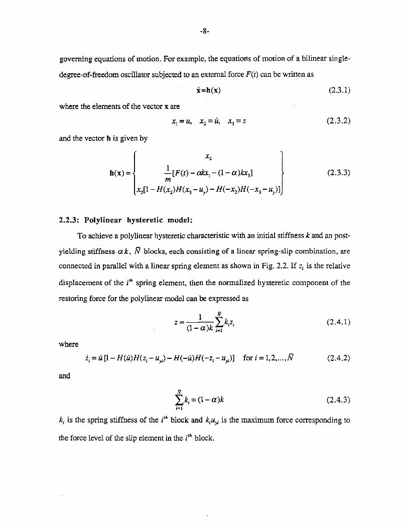


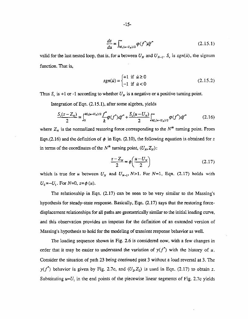


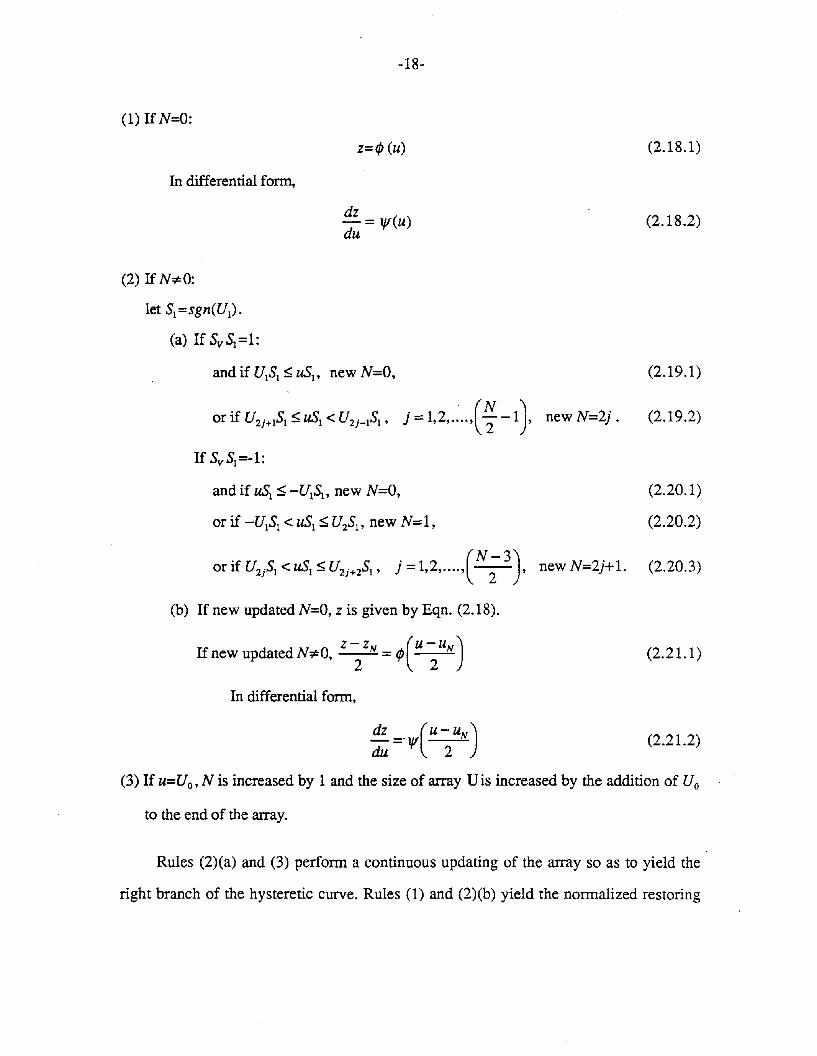

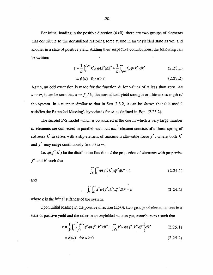


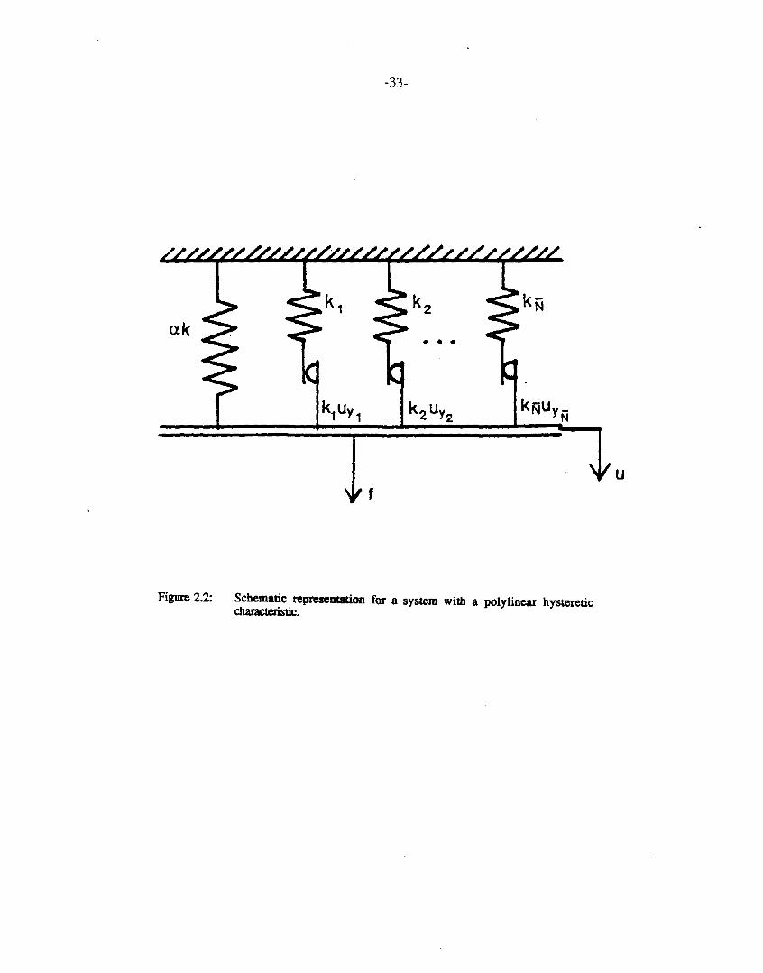


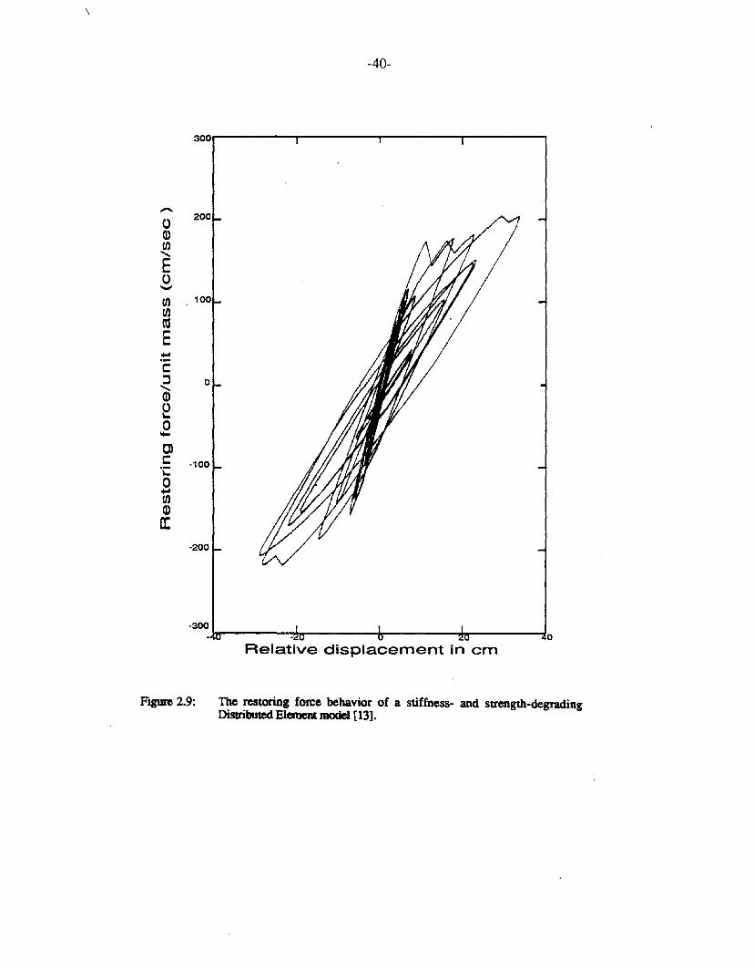


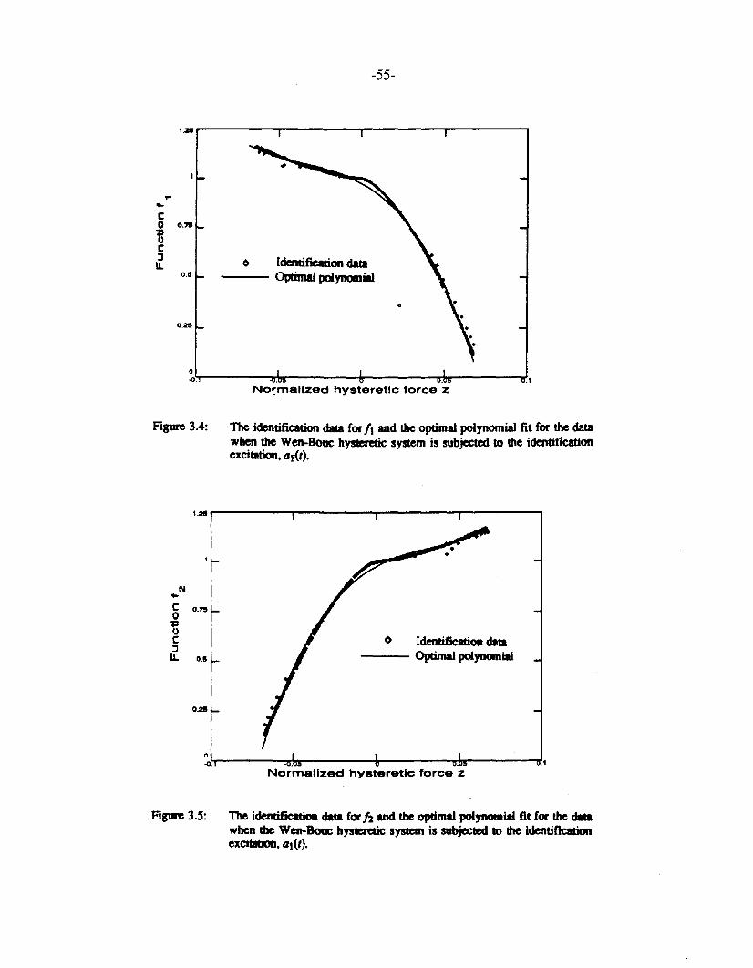


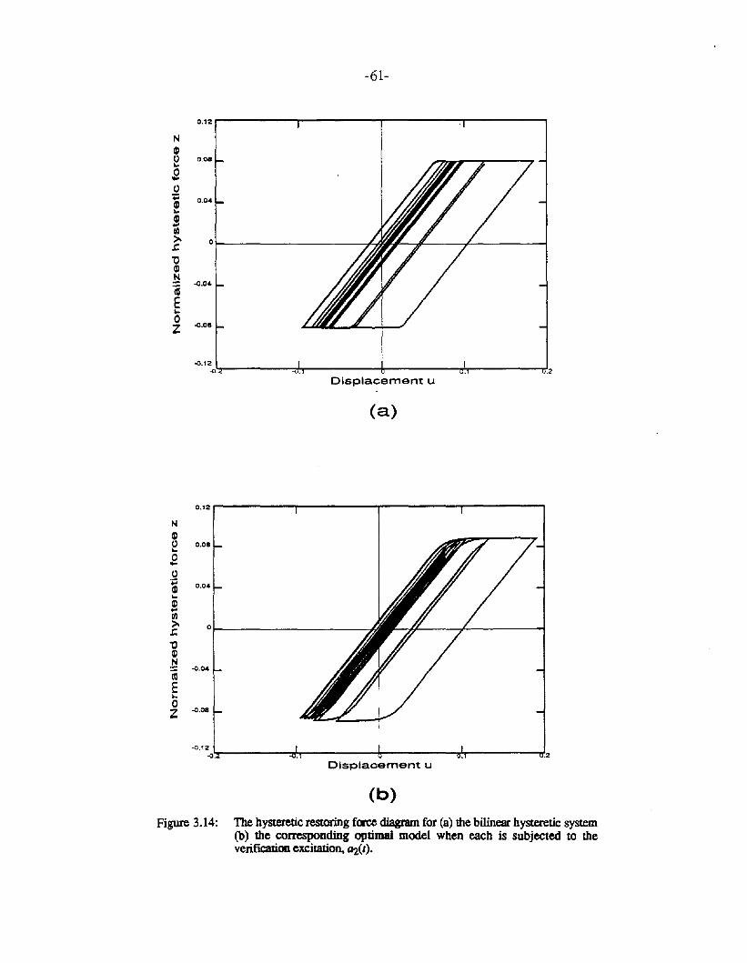


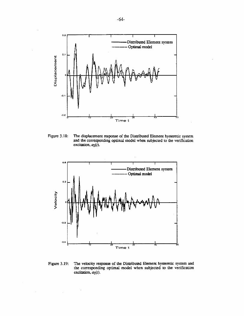


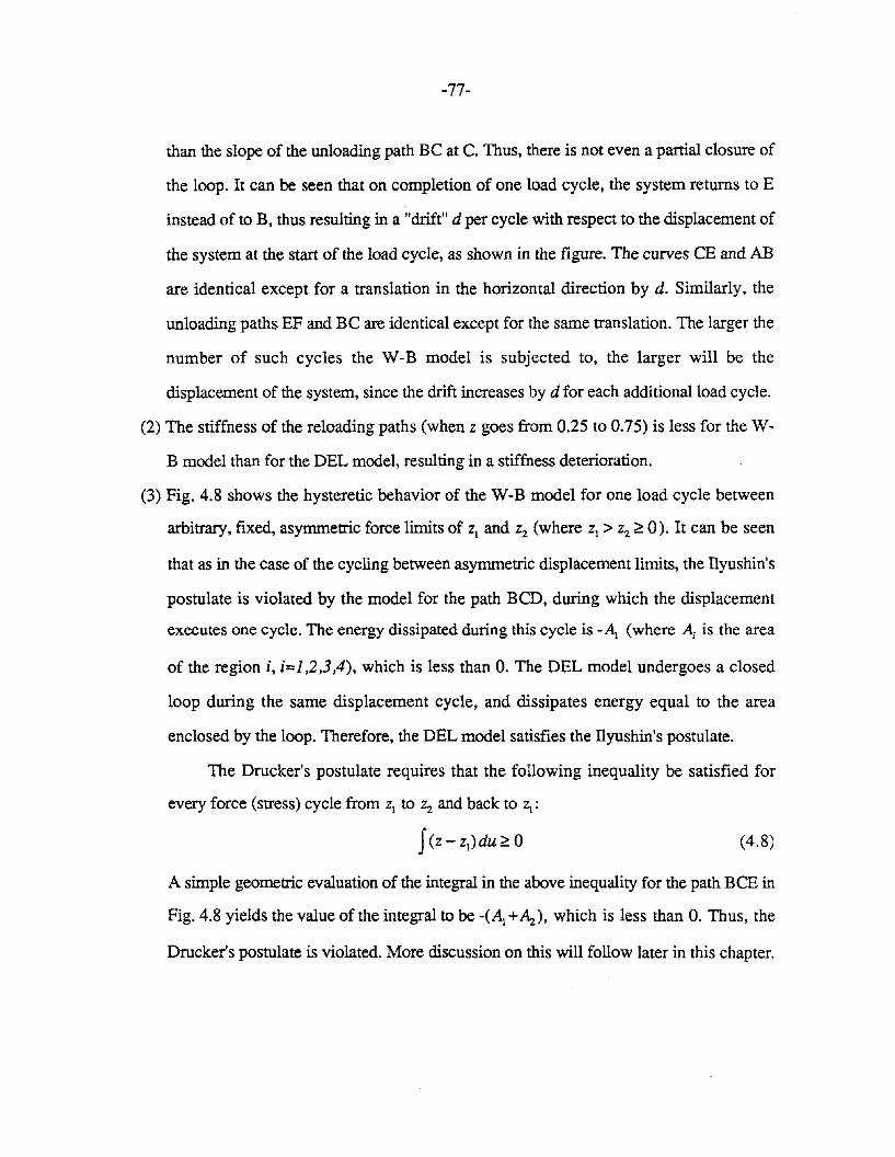
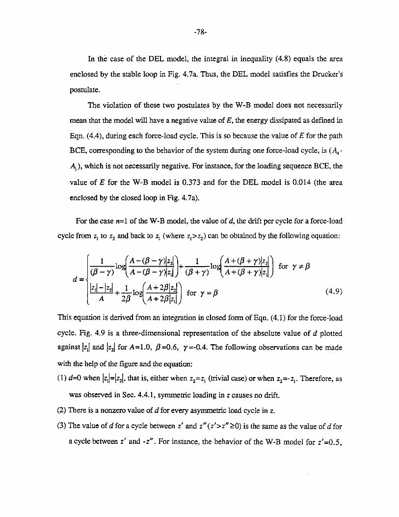


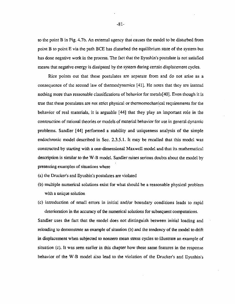


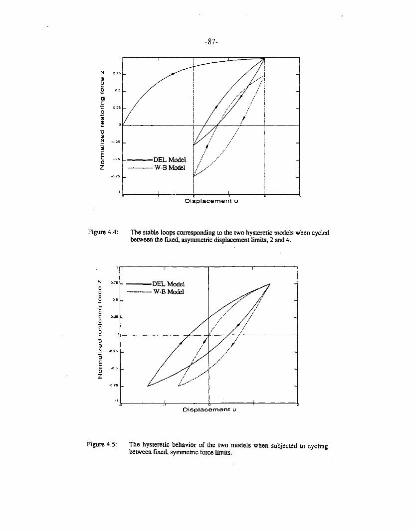

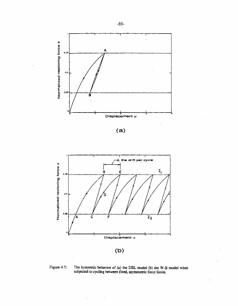


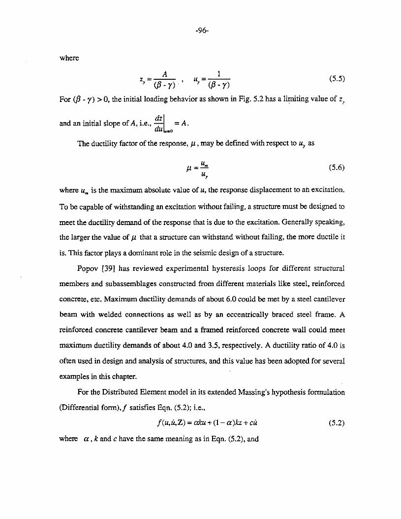

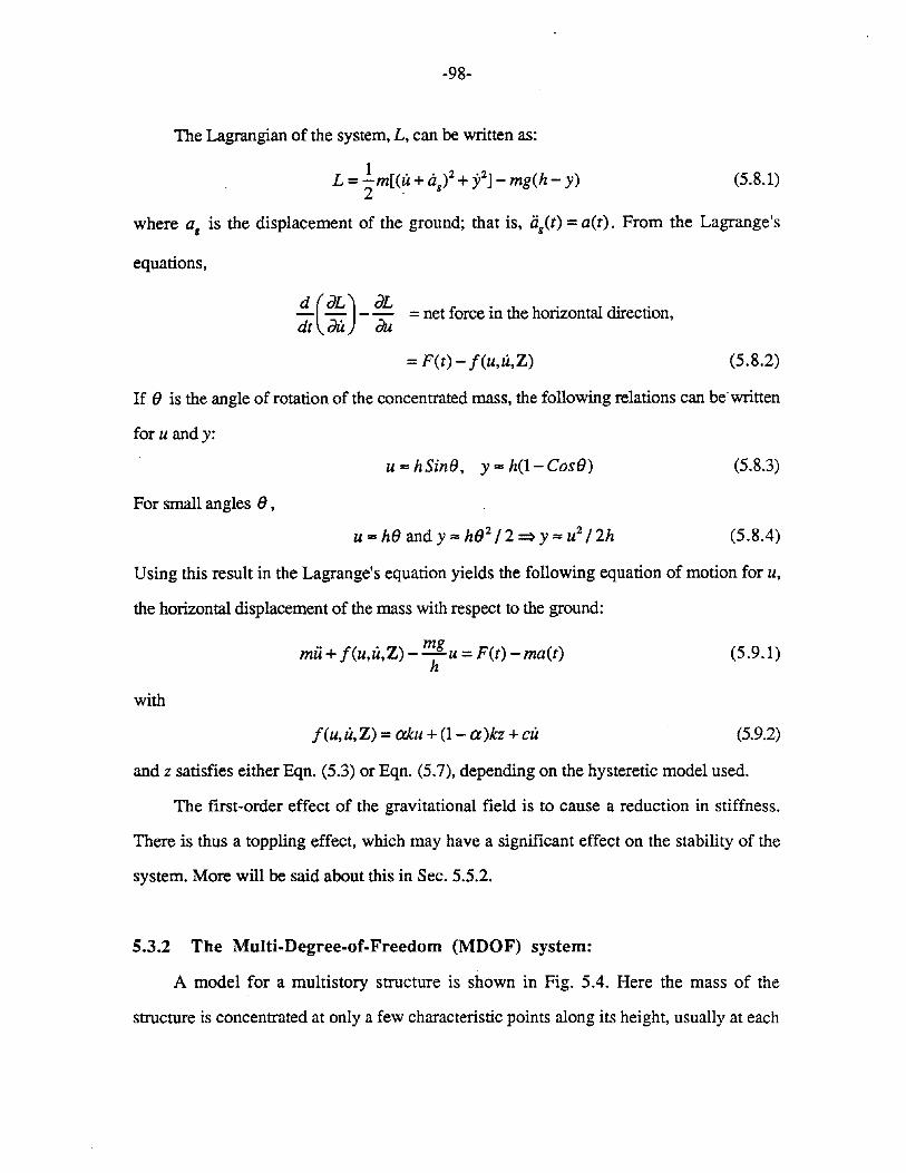


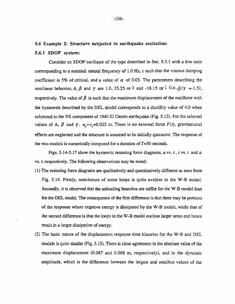

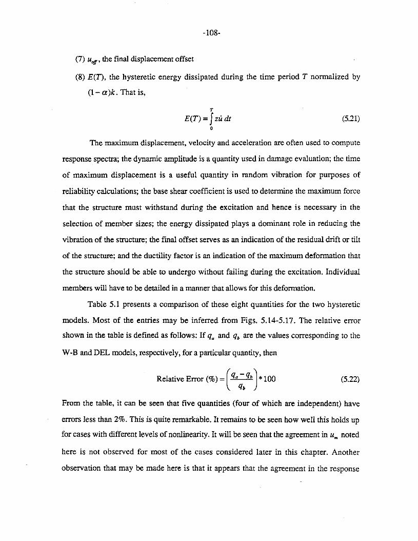


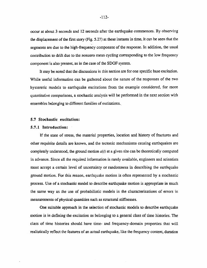


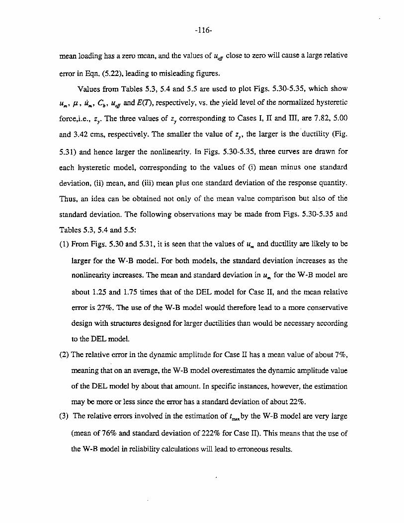


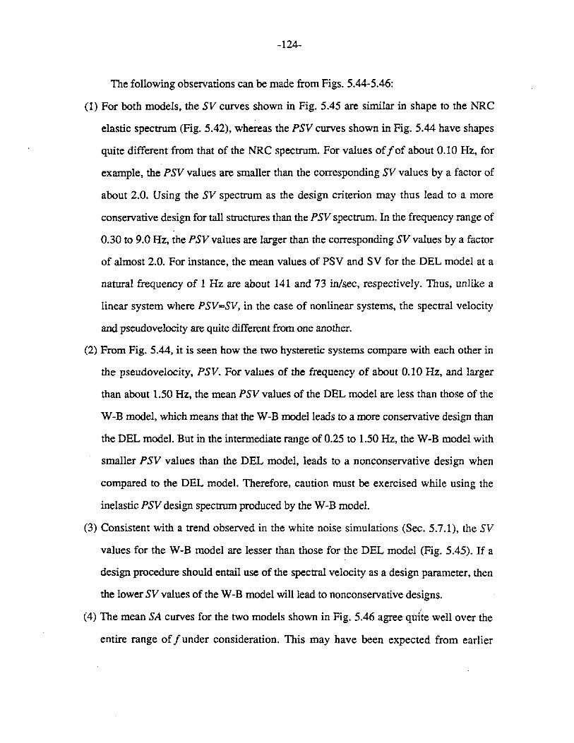


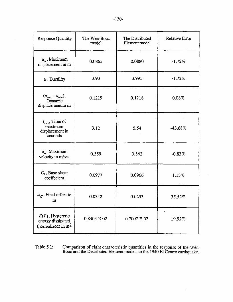


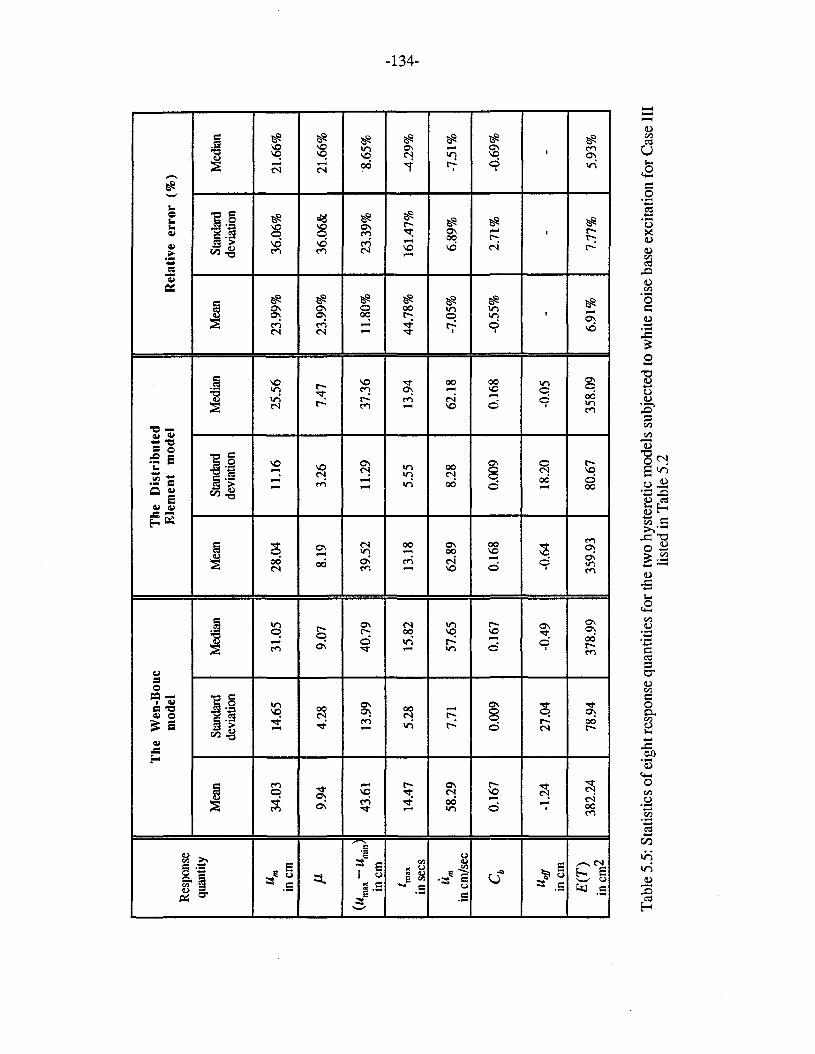


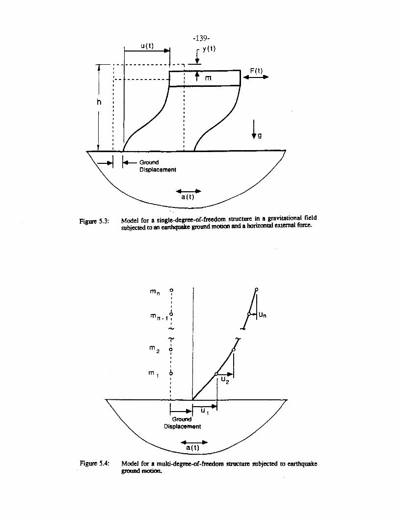


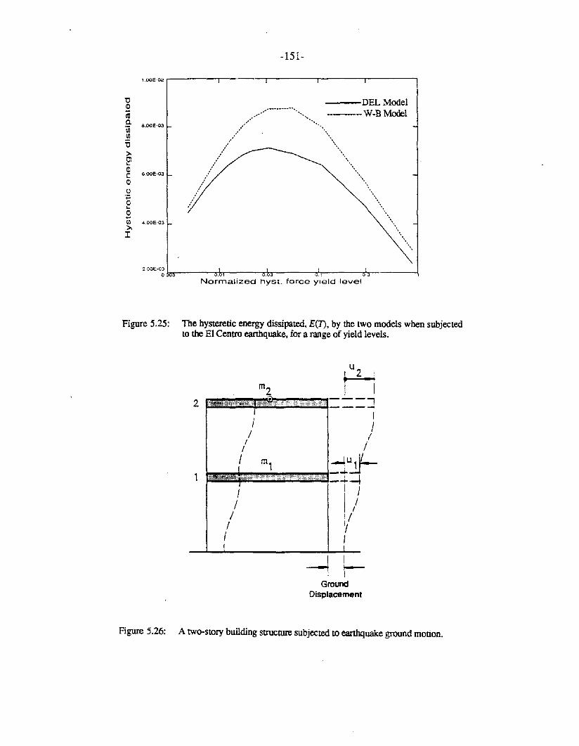

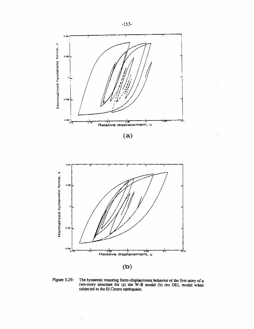


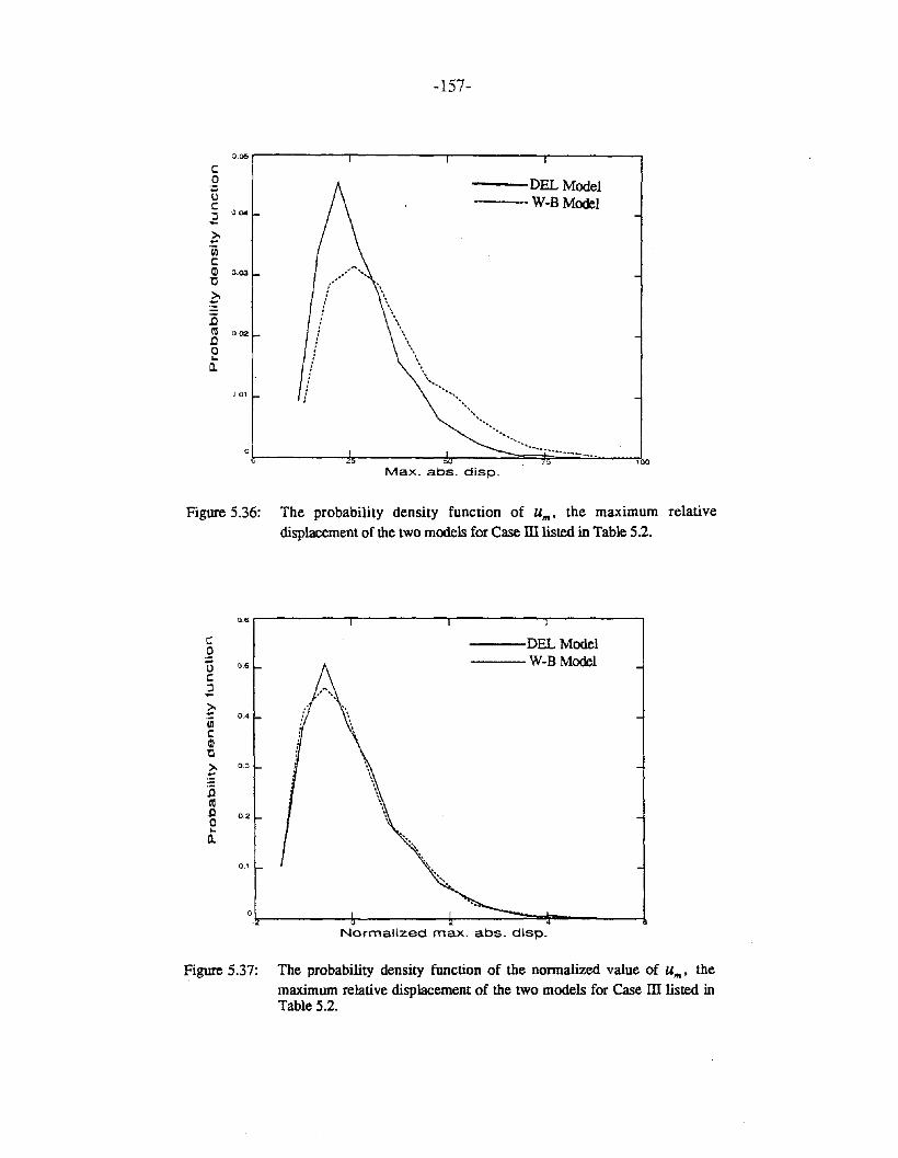


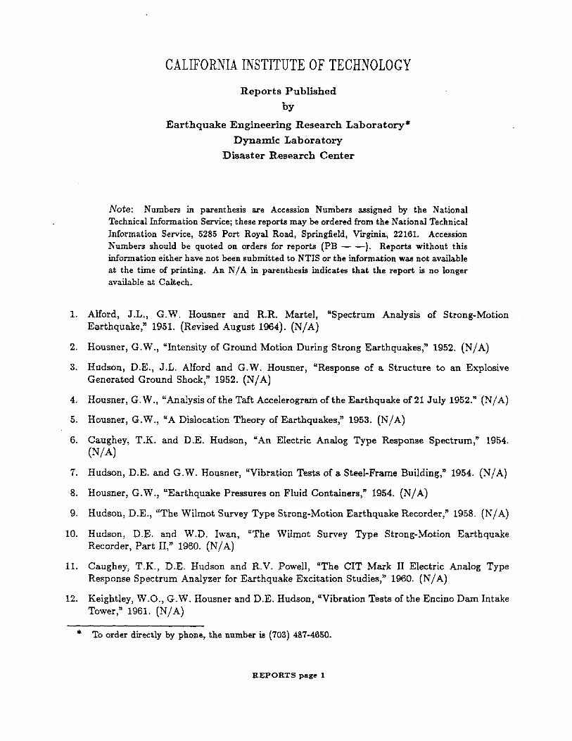


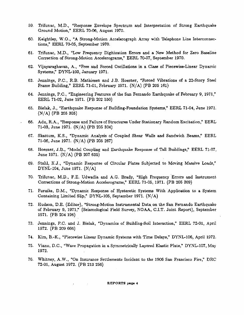


![Journal of Constructional Steel Researchdownload.xuebalib.com/xuebalib.com.16158.pdf · infills failed by corner crushing. Markulak [10] reported the hysteretic behavior of steel](https://static.documents.pub/doc/80x56/5a78ee667f8b9a77088d4a44/journal-of-constructional-steel-lls-failed-by-corner-crushing-markulak-10-reported.jpg)


