Modeling and analysis of landscape evolution using ...

1340

ABSTRACT

Current laser scanning (Lidar, light detec-tion and ranging) technologies span a wide range of survey extent and resolutions, from regional airborne Lidar mapping and ter-restrial Lidar fi eld surveys to laboratory systems utilizing indoor three-dimensional (3D) laser scanners. Proliferation in Lidar technology and data collection enables new approaches for monitoring and analysis of landscape evolution. For example, repeat Lidar surveys that generate a time series of point cloud data provide an opportunity to transition from traditional, static representa-tions of topography to terrain abstraction as a 3D dynamic layer. Three case studies are presented to illustrate novel techniques for landscape evolution analysis based on time series of Lidar data: (1) application of multi-year airborne Lidar surveys to a study of a dynamic coastal region, where the change is driven by eolian sediment transport, wave-induced beach erosion, and human interven-tion; (2) monitoring of vegetation growth and the impact of landscape structure on overland fl ow in an agricultural fi eld using terrestrial laser scanning; and (3) investigation of land-scape design impacts on overland water fl ow and other physical processes using a tangible geospatial modeling system. The presented studies demonstrate new insights into land-scape evolution in different environments that can be gained from Lidar scanning span-ning 1.0–0.001 m resolutions with geographic information system analysis capabilities.

INTRODUCTION

Landscapes evolve over time and are subject to rapid modifi cation from natural and anthro-pogenic events. This evolution constitutes a

highly variable spatial process and, depending on selection of time intervals, spatial units, and data aggregation methods, differing or even quite opposite trends can be derived (Burroughs and Tebbens, 2008; Zhou and Xie, 2009). Com-plex spatial and temporal patterns of elevation change have been observed for stream channels (McKean et al., 2009) and for disturbed land-scapes exposed to severe erosion (Kincey and Challis, 2009). To adequately understand the mechanisms that govern landscape evolution, these processes need to be monitored at dif-ferent spatial extents, spatial resolutions, and temporal scales. By effectively doing so, poten-tial impacts from natural and anthropogenic causes can be better mitigated and predicted for regional landforms that are genetically related.

Advancements in laser scanning (Lidar, light detection and ranging) technology have enhanced our ability to measure terrestrial ele-vation. Lidar surveys generate x, y, z point cloud data that capture the structure of the terrain. From these measurements, digital elevation models (DEMs) can be derived and other meth-ods employed to analyze changes in surfaces for a variety of applications (e.g., White and Wang, 2003; Hollaus et al., 2005; Bellian et al., 2005; Afana et al., 2010). With the proliferation in Lidar systems and data, there is a need for new terrain analysis methods that can more effec-tively exploit and integrate information col-lected from different Lidar modalities (Large et al., 2009). Current laser scanning technolo-gies span a wide range of survey extent, from regional airborne Lidar mapping and terres-trial Lidar fi eld surveys to ultrahigh-resolution labora tory systems utilizing indoor three-dimensional (3D) laser scanners; likewise, the achievable sampling resolutions span roughly three orders of magnitude, ranging from sub-meter to sub-millimeter, respectively (Frohlich and Mettenleir, 2004).

In this paper, three case studies are presented to illustrate the application of data acquired by three Lidar modalities for landscape evolu-tion analysis. The focus is on presenting tech-niques to incorporate and extract information from repeat Lidar surveys for different types of landscapes and at different resolutions. The fi rst case study presents an investigation of changes at a passive margin barrier island system using multiyear airborne Lidar surveys. It demonstrates the application of an analysis framework that transitions from traditional, static representations of topography to terrain abstraction as a 3D dynamic layer. The sec-ond case study presents analysis of landscape change and its impact on overland fl ow in an agricultural fi eld using terrestrial laser scan-ning. The third case study is an investigation of landscape design impacts on coastal fl ooding and water fl ow using fl exible, 3D scale models of real-world terrain that are modifi ed by the user. The impact of such modifi cations on sur-face water routing and other physical processes is analyzed using a tangible geospatial model-ing system that couples an ultrahigh-resolution laser scanner and projector with the open-source GRASS GIS (geographic resources analysis support system–geographic informa-tion system) software package (Neteler and Mitasova, 2008).

For the purposes of this paper, terrain is defi ned as bare earth surfaces combined with structures and vegetation, usually represented by a digital surface model as opposed to strictly bare earth. We consider landscape evolution as changes in the terrain that include: (1) bare earth surface change, due to natural processes such as sediment erosion and transport, or changes caused by human intervention such as grading or beach nourishment; (2) growth or decline of vegetation; and (3) construction, modifi cation, or loss of structures (e.g., buildings, roads).

For permission to copy, contact [email protected]© 2011 Geological Society of America

Geosphere; December 2011; v. 7; no. 6; p. 1340–1356; doi: 10.1130/GES00699.1; 17 fi gures; 2 tables; 1 animation.

Modeling and analysis of landscape evolution using airborne, terrestrial, and laboratory laser scanning

Michael J. Starek1, Helena Mitasova1, Eric Hardin1, Katherine Weaver1, Margery Overton2, and Russell S. Harmon 31Department of Marine, Earth and Atmospheric Sciences, and Department of Physics, North Carolina State University, Raleigh , North Carolina 27695, USA2Department of Civil, Construction, and Environmental Engineering, North Carolina State University, Raleigh, North Carolina 27695, USA3Environmental Sciences Division, Army Research Offi ce, U.S. Army Research Laboratory, Durham, North Carolina 27703, USA

Seeing the True Shape of Earth’s Surface: Applications of Airborne and Terrestrial Lidar in the Geosciences themed issue

Landscape evolution analysis with multiresolution Lidar

Geosphere, December 2011 1341

CASE STUDY 1: AIRBORNE LIDAR

Overview

Several studies have demonstrated the advan-tages of airborne Lidar surveys for monitor-ing short-term barrier island evolution, such as quantifying change in shoreline and assessing hurricane impact (e.g., Stockdon et al., 2002; Sallenger et al., 2003; White and Wang, 2003; Overton et al., 2006; Burroughs and Tebbens, 2008; Starek et al., 2009). More than 10 years of coastal Lidar mapping along the Outer Banks of North Carolina, USA, has accumulated time series of high-resolution elevation data that can be used for extraction of new information about short-term spatial patterns of coastal dynamics. However, rapid advancements in Lidar technol-ogy coupled with differences in data acquisition parameters have produced data sets with varying accuracies, scanning patterns, and point densi-ties. Therefore, geospatial analysis, when applied to decadal Lidar time series, needs to address the issues of accurate data integration and computa-tion of a consistent set of elevation models.

A Lidar point cloud processing and raster-based analysis framework for monitoring coastal landscape evolution was proposed by Mitasova et al. (2009a, 2009b). The framework introduced the concepts of core and envelope surfaces, time of elevation minimum and maxi-mum maps, and per cell analysis of elevation trends (explained in the following). These ras-ter maps preserve the spatial detail of Lidar and provide useful summary information for coastal management beyond change in shoreline or change in sediment volume.

The following case study demonstrates the application of the raster-based methodology for analyzing terrain change along the Outer Banks. The raster-based approach is further extended by representing terrain dynamics as a space-time trivariate function to generate voxel models of elevation evolution.

Study Area and Data Set

The Outer Banks are a series of barrier islands extending from Cape Henry, Virginia, to Cape Lookout, North Carolina (Fig. 1). This area has proven to be an ideal place to observe and study coastal dynamics due to rapid evolution of geomorphic features (Mitasova et al., 2009a, 2009b). Two sections along the barrier islands that have a history of beach and dune evolution as well as anthropogenic modifi cations were selected as representative locations to demon-strate the analysis approaches. Site 1 is located in the Cape Hatteras region, and site 2 is located on the southern side of Oregon Inlet (Fig. 1).

Since 1996, the Outer Banks, including Cape Hatteras, have been mapped using airborne Lidar with nearly annual frequency by sev-eral different agencies for a variety of mission objectives (Table 1). Lidar mapping with com-plete spatial coverage of the island was done in 2001 and 2008. Data sets with the most limited

coverage came from 1996 (when only the east-ern side of the island was mapped) as well as 1998 and the 2003 pre–Hurricane Isabel sur-veys, when the tip of the cape was not captured. The point data were downloaded from two online distribution sites (U.S. Geological Sur-vey Center for Lidar Information Coordination

10 kmCape Hatteras

Oregon Inlet

N

25N

USA

Canada

North Carolina

75W

80W

85W

Atlantic Ocean

40N

Jockey’s Ridge

Figure 1. Locations of the study sites on the Outer Banks, North Carolina, USA.

TABLE 1. AIRBORNE LIDAR SURVEYS

metsysradiLsetad,ycnegAVertical accuracy*

(m)Point density*

(points/m2)NOAA, NASA, USGS

October 1996September 1997September 1998; post-Bonnie†

September 1999; post-Dennis and Floyd†

October 1999

Airborne TopographicMapper II

0.15 0.1–0.3

NCDENR, FEMA, NCFMPFebruary 2001

Leica GeosystemsAeroscan

0.20 0.1

NASA, USGSSeptember 2003 pre- and post-Isabel†

EAARL 0.15 0.2

JALBTCXAugust 2004September 2005, post-Ophelia†

CHARTS better than 0.30 2.5–4.7

NOAAMarch 2008

Optech ALTM 0.15 1.0

Note: Lidar—light detection and ranging; NASA—National Aeronautics and Space Administration; NOAA—National Oceanic and Atmospheric Administration; USGS—U.S. Geological Survey; NCDENR—North Carolina Department of Environment and Natural Resources; FEMA—Federal Emergency Management Agency; NCFMP—North Carolina Floodplain Mapping Program; JALBTCX—Joint Airborne Lidar Bathymetry Technical Center of Expertise; EAARL—Experimental Advanced Airborne Research Lidar; CHARTS—Compact Hydrographic Airborne Rapid Total Survey; ALTM—airborne laser terrain mapper.

*Accuracy based on published metadata and ground point density estimated from the data.†Hurricane names.

Starek et al.

1342 Geosphere, December 2011

and Knowledge , 2009, http://Lidar.cr.usgs.gov; National Oceanic and Atmospheric Administra-tion Digital Coast, 2010).

Raster Methods

We characterize landscape evolution over a given time period by a series of raster-based DEMs derived from Lidar surveys acquired at time snapshots tk, k = 1,…,n (Mitasova et al., 2009b). To compute a consistent time series of high-resolution DEMs from the diverse set of fi rst-return Lidar points, a processing work-flow (outlined in Mitasova et al., 2009a) is employed. The workfl ow includes analysis of point cloud properties for each survey, removal of potential systematic errors, and simultaneous interpolation of elevation rasters and smoothing of noise using regularized spline with tension (Mitasova et al., 1995).

Spatial patterns in elevation change are mapped using the resulting time series of DEMs by applying summary statistics on a per cell basis, so that each output cell in a resulting map is computed as a function of its values in the cor-responding cells across the time series. Using this approach several different types of raster maps can be generated to characterize dynamic and stable regions and extract information about change in structures and vegetation. Core sur-face (zcore) represents the minimum elevation and envelope surface (zenv) represents the maximum elevation recorded at each grid cell location (i, j)over the given study period (t1, tk):

z i j z i j t k nk kcore , min , , , ,( ) = ( ) = 1… (1)

and

z i j z i j t k nk kenv , max , , , ,( ) = ( ) = 1… . (2)

For the barrier island environment, the core sur-face represents the boundary between a dynamic layer and the stable sand volume that has not moved during the entire study period. The envelope surface represents the upper boundary between the dynamic layer and the core surface within which the topography evolved during the given time period (t1, tk). The volume bound by the core and envelope surfaces represents the space within which the actual elevation surface evolved during the study period. This 3D space is referred to as the dynamic layer (Fig. 2).

The 2D analog to the concept of dynamic layer uses specifi c contours (elevation isolines) extracted from the core and envelope surfaces to defi ne a contour evolution band within which the given contour evolved during the study period. Particularly useful for coastal analy-sis is extraction of an isoline representing the shoreline, such as a mean high water elevation contour, from the core and envelope surfaces (Fig. 2). The width of this contour band can then be used as a quantitative measure of shoreline migration range at any given location.

Spatial pattern of time associated with the core and envelope surfaces can be derived as raster maps representing time (t) of minimum elevation and time of maximum elevation:

t i j t z i j t z i jl lmax , , , ,( ) = ( ) = ( ) where env (3)

and

t i j t z i j t z i jp pmin , , , ,( ) = ( ) = ( ) where core , (4)

where values in the time maps represent the index l or p of the DEMs in the time series and the actual survey date, tl or tp, is stored as an attribute (label) for each grid cell. Map algebra can then be applied to the summary raster maps and to individual DEMs to effi -ciently extract information about discrete changes in structures (Mitasova et al., 2009b). In addition, per cell univariate statistics can be used to quantify trends in continuous eleva-tion change, such as vegetation growth or dune migration. For example, a linear regres-sion slope map represents the spatial pattern of elevation increase and/or decrease rates, and a coeffi cient of determination map represents the strength of linear dependence between time and elevation. The ability to resolve periodic change signals from more persistent trends, such as due to seasonal wave climate variation, is inherently limited by the temporal resolution of the surveys.

Space-Time Voxel Models

To extend elevation modeling with the Lidar time series beyond discrete events represented by the DEMs, land surface evolution can be modeled as a continuous trivariate function,

i-th year surface

t1t2t3..tn

result

A BFigure 2. Raster-based analysis of elevation time series. (A) Grid cell value in the resulting map is a function of grid cell values in the time (t) series. (B) Relation between a dynamic layer defi ned by core and envelope surfaces and a shoreline band, defi ned by mean high water level elevation contours extracted from the core and envelope (image courtesy of M. Onur of North Carolina State University).



z = f(x, y, t) where x, y is horizontal location, t is time, and elevation z is the modeled variable. The function f(x, y, t) is derived from a series of m point clouds {(xi, yi, ti, zi), i = 1,…, nk}tk, k = 1,…, m, where x, y, z are coordinates, nk is num-ber of points in the kth point cloud, and tk is the time of the survey. The data from all the point clouds are merged into a single point cloud

x y t z ii i i i k, , , , , ,( ) ={ }∑1… n that is then inter-polated into a 3D raster (voxel model) using a trivariate interpolation method (Fig. 3).

The extension of spatial interpolation tech-niques z = f (x, y) to the space-time domain z = f (x, y, t) is not a simple matter of adding another dimension for time, as there are fun-damental differences between the space and time domain (Kyriakidis and Journel, 1999). Space represents a state of coexistence in which there can be multiple dimensions and no direct concept of ordering is present. In contrast, time represents a state of successive existence where a clear ordering (nonrevers-ible) in only one dimension is present, there are often periodic components, and extrapolation is usually of main interest (Snepvangers et al., 2003). In our case, the trivariate regularized smoothing spline with tension (Mitasova et al., 1995) includes an anisotropy parameter that is applied to the time dimension for interpolation of a space-time voxel model. The function has the following form:

z ar

erfr

jj

N

= +

−

=∑λ π

ϕϕ

22

21

, (5)

where r x x y y t tj j j= −( ) + −( ) + −( )2 2 2θ is

the distance between the voxel grid point (x, y, t) and the given point (xj, yj, tj), a is constant trend term, ϕ is tension parameter, θ is anisotropy parameter in time dimension, λj are coeffi cients solved through a linear system of equations, and erf(.) is the error function (Weisstein, 2011). The implementation of the trivariate spline function in GRASS GIS (Neteler and Mitasova, 2008) includes a smoothing parameter, often needed when processing noisy Lidar data time series. To support processing of merged point clouds the data are interpolated using an octree segmentation procedure. Time resolution is selected to be close to the time interval of the surveys, although the approach is designed to handle irregular time intervals as well.

Evolution of a given contour z = c can then be visualized as an isosurface extracted from the voxel model. For example, shoreline evo-lution can be represented by the isosurface z = zMHW where zMHW is the mean high water eleva-tion level. This visualization concept is similar to the space-time cube approach proposed for epi demiologic studies (Kraak and Madzudzo, 2007) or remote sensing meteorological data (Turdukulov et al., 2007).

Examples

Cape HatterasCape Hatteras is a highly dynamic region of

the Outer Banks that migrates in response to eolian forces, the meeting of the Gulf Stream

and the Labrador Current, and the subsequent exchange of sediment between the Diamond Shoals and the beaches along the cape (Fig. 1). Furthermore, the area is frequently subject to winter storms and hurricanes. The terrain was notably altered in 2003 when Hurricane Isabel caused major beach and dune erosion through-out Hatteras Island and carved an inlet between the towns of Hatteras and Frisco. Shortly after, the near-island bathymetry and local topography was again altered when the U.S. Army Corps of Engineers fi lled the inlet and reconstructed the dune ridge.

To assess landscape dynamics in the region, 0.5 m resolution DEMs were generated from the 1996–2008 Lidar time series and subsequently used to generate raster summary maps. The time of minimum and maximum elevation maps shows that much of the area on the eastern side of Cape Hatteras near the shoreline was at its maximum elevation during the earlier years in the study and at its minimum during the later years (i.e., 2008; Fig. 4). This indicates an erosive trend for the eastern side of the cape and suggests that the cape is accreting toward the west. In addition, the diversity of years when the elevation was at maximum near the tip of the cape captures well the dynamic nature of the region, and is further demonstrated in Figure 5, which shows the rela-tion between the envelope surface and core sur-face. The distance between the minimum and maximum shorelines (>1 km over an ~10 yr period) illustrates the large magnitude of sedi-ment transport that occurs on Cape Hatteras.

space-time elevation cube

t1

t2

tm

1570 m

interpolatez = f(x, y, t)

(x, y, z)

…

reorderas

(x, y, t, z)

z-value at (x, y, tk)

Time t(year)

y (m)

x (m)

(x, y, z)

(x, y, z)

Figure 3. Representation of terrain evolution using the trivariate space-time function: merged time series of point clouds is interpolated into space-time voxel model (see text).

Starek et al.


Oregon InletLandscape evolution on the south side of

Oregon Inlet (Figs. 1 and 6A) was analyzed (Mitasova et al., 2009a) for the time period 1997–2005. That analysis is extended here by adding data from a year 2008 Lidar survey and by representation of topographic evolution in the area using a space-time voxel model. Fig-ure 6B shows shoreline evolution represented as a set of mean high water elevation (0.3 m) contours referenced to the North American Vertical Datum of 1988 (NAVD 88). Interpre-tation of the shoreline dynamics alongshore during the study period becomes diffi cult with this 2D contour representation. In comparison, elevation isosurfaces extracted from the vol-ume representation provide interesting insight

into coastal dynamics in the region. Figure 6C shows mean high water shoreline evolution represented as a 0.3 m elevation isosurface. This isosurface exhibits very complex geom-etry, suggesting a rapidly evolving foreshore region due to shoreline erosion and sand dis-posal in the area. In addition, the 5 m and 8 m elevation isosurfaces were extracted to repre-sent lower and higher foredunes in the region (Fig. 7). Contours within this range of eleva-tion demonstrated the most interesting patterns in the isosurfaces (Fig. 8). For example, if the extracted contour represents elevation close to a foredune ridge, “holes” in the isosurface represent temporal loss of elevation that has recovered. Such holes typically arise from an overwash after which the dune was repaired or

recovered. This pattern is shown in Figure 7B for the 5 m surface in a region where an over-wash occurred in 2003 (Fig. 7A). In contrast, the 8 m contour revealed the most stable dune peaks in the area (Fig. 7C).

The presented raster and space-time voxel model methodologies are general and can be used with any software that supports raster data processing and/or trivariate interpolation for voxel model generation. Our implementa-tion was based on the open source GRASS GIS (Neteler and Mitasova, 2008; for more details and additional applications, see Mitasova et al., 2009a, 2009b, 2011).

CASE STUDY 2: TERRESTRIAL LIDAR

Overview

Terrestrial Lidar, commonly referred to as terrestrial laser scanning (TLS), has lagged behind airborne Lidar in its utilization for ter-rain mapping (Buckley et al., 2008). Since the introduction of the fi rst commercial systems in the late 1990s (Petrie and Toth, 2009), ter-restrial Lidar has seen continued development and growth; however, only within the last few years has the technology evolved to be robust and compact enough for practical use in many environ ments (Buckley et al., 2008). This expansion has been further propelled by the development of software capable of effi ciently dealing with the massive, complex nature of true 3D point cloud data. Today, terrestrial Lidar is evolving at a brisk pace in terms of size, cost, and measure ment capabilities (e.g., full-wave-form systems are now on the market), and it is fi nding increasing application in many diverse areas of earth science research (e.g., Pringle et al., 2004; Bellian et al., 2005; Hetherington et al., 2007; Bonnaffe et al., 2007; Buckley et al., 2008; Heri tage and Milan, 2009; Olsen et al., 2009; James et al., 2009; Fernandez et al., 2010; Smith et al., 2011).

TLS for Monitoring Agricultural LandscapeAgricultural practices alter the hydrologic

system in a watershed and are widely recog-nized as being capable of accelerating soil loss (Montgomery, 2007; Wilkinson and McElroy , 2007; Pimentel et al., 1995). The major infl u-ence of landscape structure, i.e., the spatial organization of land units with different land uses, size, fi eld boundaries, roughness, slope gradient, and the connectivity between them, on surface runoff and sedimentation pat-terns within agricultural land is well docu-mented (e.g., Ludwig et al., 1995; Vandaele and Poesen, 1995; Govers et al., 1994; Van Oost et al., 2000). These results emphasize the

A BFigure 4. Raster maps of Cape Hatteras region generated from the Lidar time series. Dennis, Floyd, and Isabel are hurricanes. (A) Time when the elevation was at its minimum draped as a color map over the core surface. (B) Time when elevation was at its maximum draped as a color map over the envelope surface.

Figure 5. Cape Hatteras: enve-lope surface (green) is cut away to reveal the core surface (red). The distance between the mini-mum (white) and maximum (green) shorelines illustrates the extent of shoreline change that occurs on Cape Hatteras.



0

1 km

Ore

gon

Inle

t

z=

0.3

m

wav

essand

dis

posa

l

soun

d

beac

h

x(m

)

A

CB

Tim

e(y

ear)

y(m

)

2008

2005

2003

2001

1999

1997

Dis

tanc

e

75 90 105

120

135

150

mYea

r

1997

1999

2001

2003

2005

2008

shor

elin

e

Fig

ure

6. S

hore

line

evol

utio

n in

spa

ce-t

ime

cube

(see

text

). (A

) Lid

ar s

urfa

ce d

igit

al e

leva

tion

mod

el s

how

ing

coas

tlin

e ne

ar O

rego

n In

let,

Nor

th C

arol

ina,

in 2

008.

Box

sho

ws

regi

on o

f ana

lysi

s. (B

) Mea

n hi

gh w

ater

(MH

W) s

hore

line

evol

utio

n re

pres

ente

d as

a s

et o

f 0.3

m c

onto

urs.

(C) C

onto

ur is

osur

face

sho

win

g th

e dy

nam

ic m

ovem

ent (

retr

eat o

r ad

vanc

e) o

f the

MH

W s

hore

line

duri

ng th

e st

udy

peri

od; c

olor

rep

rese

nts

the

dist

ance

from

the

base

line

show

n as

the

whi

te li

ne in

B.

Starek et al.


need to be able to measure landscape changes within and across agricultural lands to better assess the impact of agricultural practices on hydrologic processes. In this regard, TLS offers great potential as a rapid measurement technology for quantifying microtopographic and land cover changes within an agricultural fi eld; however, the utilization of laser scanning for this application has been relatively limited (Afana et al., 2010).

In the following case study, results of the application of repeat TLS surveys to monitor elevation change in vegetated surfaces within an agricultural fi eld are presented. The impact of the landscape structure and influence of measure ment scale on spatial patterns in over-land fl ow are then investigated using GIS-based fl ow simulation.

Study Area

North Carolina State University maintains an experimental agricultural fi eld called the Sediment and Erosion Control Research and Education Facility (McLaughlin et al., 2001) (Fig. 9). The fi eld is located within the eastern edge of the Piedmont foothills region of North Carolina (star in Fig. 1). The fi eld comprises a catchment for two subwatersheds and was subjected to rill erosion along the hillsides during heavy rain events and gully erosion within a drainage basin formed by the con-fl uence of runoff from two main hillslopes (Fig. 9). The fi eld consists mostly of dense grassland, but it is subjected to anthropogenic modifi cation by tillage and other agricultural practices. For this study, an ~250 m × 100 m

area that includes a tilled and nontilled region was selected for monitoring by terrestrial laser scanning (Fig. 9).

Data Acquisition Methods

One of the principal advantages of TLS com-pared to its airborne counterpart is the ability to rapidly acquire dense 3D measurements of the land surface; however, there are inherent limi-tations that must be considered for application to dynamic terrain monitoring. Because such systems have limited scanning ranges (typically a few hundred meters or less) and are static, multiple scans must be merged together to form a seamless model of the terrain scene. For contigu ous mapping of terrain over wide areas (greater than a few hundred meters), this poses

C

z = 8 m

stable dune peaks

B

DEM (year)

2005

2003

1997

A0 200 m

Year

1997

1999

2001

2003

2005

2008

dune overwash

z = 5 m

Figure 7. Evolution of the foredune near Oregon Inlet, North Carolina. (A) Three snapshots from bare earth digital elevation model (DEM) time series illustrating changes in the beach-foredune system, including an overwash in the year 2003. (B) Evolution of a 5.0 m contour displayed as isosurface; holes (ellipse) represent the dune overwash caused by Hurricane Isabel in 2003, after which the dune was repaired. (C) Evolution of an 8.0 m contour displayed as isosurface representing the highest dune peaks along this stretch of beach.



several obstacles that must be overcome. The selected measurement setup, sampling resolu-tion, and other survey design factors, as well as inherent system characteristics, will infl uence the measure ment capabilities and effi ciency of repeat-coverage terrestrial Lidar surveys (Buck-ley et al., 2008). The measurement uncertainty, stemming from the system and survey char-acteristics, will directly propagate into DEMs derived from the data and subsequent change detection analysis (Wheaton et al., 2010). Therefore, development of a consistent frame-work for TLS data acquisition and processing is vital for utilization of the technology for moni-toring subtle changes in the landscape (Hether-ington et al., 2007; Buckley et al., 2008).

Surveys of the study region were conducted using a Leica Geosystems ScanStation 2 terres-trial laser scanner. The ScanStation 2 operates at a 50 kHz pulse rate and records a single return per an outgoing pulse (see Table 2 for system specifi -cations). Due to the low look angle of the scanner relative to the refl ecting land surface, limitations in the scanner range and fi eld-of-view, and varia-tion in surface topography, certain regions of the ter-rain scene will be occluded from the view of the scanner depending on where the scan is acquired.

Figure 8. Evolution of elevation contours alongshore displayed as isosurfaces: 0.3, 0.9, 1.5, 1.8, 2.1, 2.7, 3.0, 3.7, 4.5, 5.5, 6.5, 7.5, 9.0 m. This fi gure is intended to be viewed as an ani-mation. For the animated .gif fi le, please visit http://dx.doi.org/10.1130/GES00699.S1 or the full-text article on www.gsapubs.org to view the animation.

0 200 m

NA

B

Figure 9. (A) Experimental agricultural fi eld with an orthophoto draped over an airborne Lidar-derived 1-m-resolution digital eleva-tion model (DEM; area is ~450 × 450 m2). The shaded region is the focus of the study area that includes tilled portions of the fi eld and the main drainage outlet (star). (B) 1 m Lidar-derived bare earth DEM showing difference between vegetation coverage and terrain.

Starek et al.


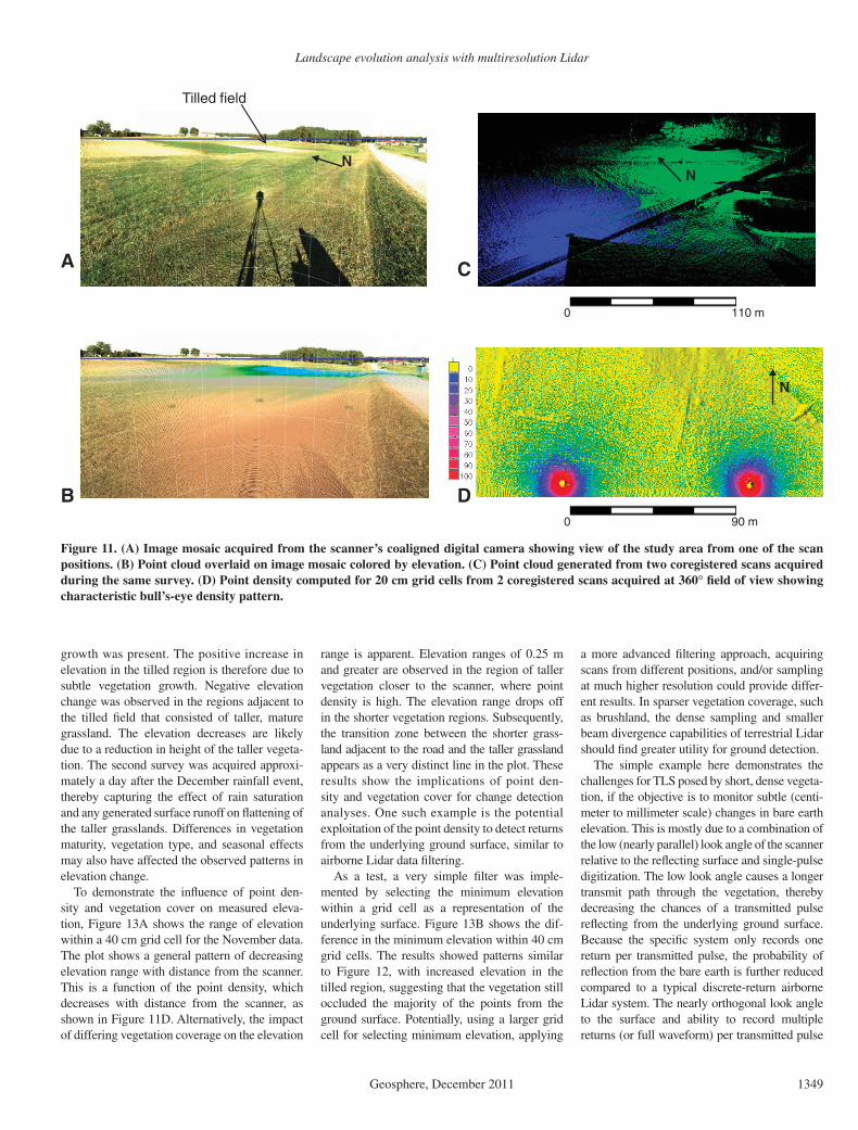
Because of these inherent system limitations, viewshed analysis using a 1 m airborne Lidar-derived DEM of the study region was performed within GRASS GIS (Neteler and Mitasova, 2008) to simulate data acquisition at different scan posi-tions (Fig. 10). An optimization approach was then implemented to determine favorable scan positions based on cumulative viewsheds (Starek et al., 2010). From this approach, two scan posi-tions ~100 m apart were selected for monitoring the study region (Figs. 11A–11C).

Scans collected for a given survey must be coregistered together and subsequently refer-enced relative to other surveys across time with great accuracy to be able to effectively mea-sure subtle changes in the landscape. Absolute georeferencing is therefore not important for change detection so long as the scans are ref-erenced rela tive to each other within a localized coordinate frame (Fig. 11C). A systematic data acquisition and registration scheme was devel-oped whereby scans for a given survey were fused together using shared targets set up during the survey and acquired within the data point clouds. The scans were then precisely referenced relative to each other across time using cloud-to-cloud registration based on static objects in the scene (e.g., corners of buildings, fence posts). The processing was performed using the Leica Cyclone software module. The registration framework provided mean absolute positional errors of <1 cm for target-to-target scan registra-tion and <2 cm for cloud-to-cloud registration between surveys across time. Vertical positional

errors were within ~6–8 mm based on compari-son of the vertical component of control points between surveys. Assuming a vertical error of σz = 6 mm, and propagating the error due to the differencing of two vertical measurements, σ σ σuncertainty = +z z1

22

2 , this equates to a verti-cal uncertainty in change detection of ~8.4 mm (Wheaton et al., 2010).

Scans were acquired with an average sam-pling resolution of 1 cm spacing at 10 m range, resulting in very dense sampling near the scan-ner and within regions of overlapping clouds. Progressive decreasing in sampling resolution moving away from the scanner forms a bull’s-eye density pattern, as shown in Figure 11D, that is characteristic of a two-degree-of-freedom oscillating mirror scanner commonly employed in terrestrial Lidar systems. The point density and high accuracy registration enabled subtle (centimeter to sub-centimeter level) changes in the landscape to be measured.

Change Detection

Several TLS surveys were conducted at the study site, ranging in temporal spans from approximately one to three months. Surveys were directed toward major rainfall events, sea-sonal vegetation changes, and agricultural oper-ations. The results shown here are based on two surveys conducted on 3 November 2009 and 4 December 2009. During this one month span, ~12.7 cm of rainfall was recorded at the site (North Carolina State Climate Offi ce, 2011). Two main rainfall events occurred during the period. On 10–11 November, a total of 6.35 cm fell over an ~17 h period with a maximum inten-sity of 0.69 cm/hr. On 2–3 December, a total of 5 cm fell over an ~13 h period with a maximum intensity of 1.45 cm/hr.

To quantify changes in the landscape, DEMs were generated for each survey at 20 cm reso-lution using regularized spline under tension within GRASS GIS (Neteler and Mitasova, 2008). The DEMs were then differenced to measure change in elevation between the two surveys. No tillage operations or other agri-cultural practices occurred during the period between our two surveys; therefore, changes in the bulk density of the surface associated with tillage loosening the soil or compaction from farm machinery were not directly observed.

Figure 12 shows the change in elevation measured between the two surveys. Positive ele-vation change was observed in the recently tilled fi eld (Fig. 12), where the most potential for ero-sion would be expected due to the least mature vegetation coverage. However, by the time the first survey was acquired, initial vegetation

N

0 150 m

Figure 10. Impact of elevation surface geometry on spatial extent of a single scan: signifi -cant difference in viewsheds computed from two scan positions located in close proximity to each other.

TABLE 2. LEICA SCANSTATION 2 SPECIFICATIONS

neerGresalR3ssalCBeam divergence 0.15 mradPulse rate (pulses/s) ≤ 50,000Field of view (degrees) 360 × 270 Range at 90% albedo; 18% albedo 300 m, 134 mSpot size* ≤ 6 mmAccuracy (position†, distance†) 6 mm, 4 mmPoint spacing (minimum) < 1 mmDual axis tilt compensator 1″ resolution

*From 0 to 50 m based on Gaussian defi nition.†1 m to 50 m range, 1 sigma.



growth was present. The positive increase in elevation in the tilled region is therefore due to subtle vegetation growth. Negative elevation change was observed in the regions adjacent to the tilled fi eld that consisted of taller, mature grassland. The elevation decreases are likely due to a reduction in height of the taller vegeta-tion. The second survey was acquired approxi-mately a day after the December rainfall event, thereby capturing the effect of rain saturation and any generated surface runoff on fl attening of the taller grasslands. Differences in vegetation maturity, vegetation type, and seasonal effects may also have affected the observed patterns in elevation change.

To demonstrate the infl uence of point den-sity and vegetation cover on measured eleva-tion, Figure 13A shows the range of elevation within a 40 cm grid cell for the November data. The plot shows a general pattern of decreasing elevation range with distance from the scanner. This is a function of the point density, which decreases with distance from the scanner, as shown in Figure 11D. Alternatively, the impact of differing vegetation coverage on the elevation

range is apparent. Elevation ranges of 0.25 m and greater are observed in the region of taller vegetation closer to the scanner, where point density is high. The elevation range drops off in the shorter vegetation regions. Subsequently, the transition zone between the shorter grass-land adjacent to the road and the taller grassland appears as a very distinct line in the plot. These results show the implications of point den-sity and vegetation cover for change detection analy ses. One such example is the potential exploitation of the point density to detect returns from the underlying ground surface, similar to airborne Lidar data fi ltering.

As a test, a very simple fi lter was imple-mented by selecting the minimum elevation within a grid cell as a representation of the underlying surface. Figure 13B shows the dif-ference in the minimum elevation within 40 cm grid cells. The results showed patterns similar to Figure 12, with increased elevation in the tilled region, suggesting that the vegetation still occluded the majority of the points from the ground surface. Potentially, using a larger grid cell for selecting minimum elevation, applying

a more advanced fi ltering approach, acquiring scans from different positions, and/or sampling at much higher resolution could provide differ-ent results. In sparser vegetation coverage, such as brushland, the dense sampling and smaller beam divergence capabilities of terrestrial Lidar should fi nd greater utility for ground detection.

The simple example here demonstrates the challenges for TLS posed by short, dense vegeta-tion, if the objective is to monitor subtle (centi-meter to millimeter scale) changes in bare earth elevation. This is mostly due to a combination of the low (nearly parallel) look angle of the scanner relative to the refl ecting surface and single-pulse digitization. The low look angle causes a longer transmit path through the vegetation, thereby decreasing the chances of a transmitted pulse refl ecting from the underlying ground surface. Because the specifi c system only records one return per transmitted pulse, the probability of refl ection from the bare earth is further reduced compared to a typical discrete-return airborne Lidar system. The nearly orthogonal look angle to the surface and ability to record multiple returns (or full waveform) per transmitted pulse

Tilled field

A

B

C

D

NN

N

0 90 m

0 110 m

Figure 11. (A) Image mosaic acquired from the scanner’s coaligned digital camera showing view of the study area from one of the scan positions. (B) Point cloud overlaid on image mosaic colored by elevation. (C) Point cloud generated from two coregistered scans acquired during the same survey. (D) Point density computed for 20 cm grid cells from 2 coregistered scans acquired at 360° fi eld of view showing characteristic bull’s-eye density pattern.

Starek et al.


increases the probability of bare earth detection for airborne systems. In this regard, develop-ments in full-waveform terrestrial Lidar may fi nd potential application.

The maximum rainfall duration and intensity events that occurred between the surveys were not substantial enough to generate measurable soil erosion or deposition within the dense grass cover at the study site. Therefore, our objective here was to demonstrate the utility of TLS for monitoring changes in vegetation cover within an agricultural fi eld. Although the bare earth at the study site was occluded by vegetation, the underlying topographic sig-nature is still captured by terrestrial Lidar as well as the spatial organization of the different land units, tillage patterns, and the connectiv-ity between them. This landscape structure information provides valuable information for assessing spatial patterns in overland fl ow, as discussed in the following.

Flow Pattern Analysis

Topographic parameters (e.g., slope gradients and curvatures), variations in surface rough-ness induced by water erosion and agricultural practices (e.g., rills and tillage), fi eld bound-aries, random microscale topographic variations (e.g., distribution of clods and aggregates on a surface), and vegetation coverage play impor-tant roles in controlling overland fl ow patterns within an agricultural catchment (Darboux et al., 2002). The ability of TLS to capture microscale (<1 m) and macroscale (>1 m) variations in the terrain provides an exceptional data source for modeling spatial patterns in overland fl ow. This approach can be further used in a change detec-tion capability to determine which subtle terrain changes measured between terrestrial Lidar sur-veys are infl uential to the overall fl ow patterns in the fi eld.

To assess the impact of measurement scale and the observed terrain changes on spatial patterns in overland fl ow, the 20-cm-resolution DEMs generated from the TLS surveys on 3 November 2009 and 4 December 2009 were used to derive overland fl ow patterns using the D-infi nite fl ow tracing algorithm implemented in r.fl ow module in GRASS GIS (Neteler and Mitasova, 2008). These results were then com-pared to overland fl ow results based on a 1 m airborne Lidar-derived DEM of the agricultural fi eld. Figure 14 compares the results obtained from TLS and airborne Lidar; the most notable is that terrestrial Lidar captures preferential fl ow patterns due to tillage and its persistence across time. Airborne Lidar captures general fl ow pat-terns within the main drainage outlet and along the fi eld boundary at the edge of the road, but

even at 1 m resolution, airborne Lidar fails to capture the majority of fl ow patterns due to till-age and other microtopographic variations. It is evident from the results the potential value TLS can provide for monitoring land surface changes within an agricultural fi eld due to both natural and anthropogenic forcing. Results such as these obtained by TLS can in return aid researchers in determining important terrain features infl uen-tial to the soil erosion processes to direct mitiga-tion efforts and assess their effectiveness.

CASE STUDY 3: LABORATORY LIDAR

The previous sections focused on the analysis of the landscape state and dynamics as captured by airborne or terrestrial Lidar surveys using digital (virtual) terrain models representing real-world topography. However, there are many applications, such as in land use management, landscape design, military installation opera-tional planning, or education, where modifi ed terrain conditions and their impact on landscape processes need to be evaluated, often in a col-

laborative environment. The tangible geospatial modeling system (TanGeoMS; Tateosian et al., 2010) couples an ultrahigh-resolution (sub-milli-meter) 3D laser scanner, projector, and a fl exi-ble physical 3D model with a standard GIS (in our case GRASS; Neteler and Mitasova, 2008) to create a tangible interface for landscape anal-ysis (Fig. 15A). The 3D physical scale model is constructed to have a soft malleable surface that can be modifi ed by hand to create various landscape confi gurations. For example, surface depressions can be pushed in to create ponds and stream channels, dams and levees can be added, buildings can be introduced, and the surface roughness can be modifi ed to represent vegetation or other properties by simple addi-tions of clay and other materials. The scaled models are derived from real-world data, such as from topographic contours generated from a bare earth Lidar-derived DEM, and the desired accuracy of the model can be adjusted using the projected differences between the original and georeferenced scanned model elevations (Mitasova et al., 2011).

A B

Tilled field

N

0 30 60 120 180 m

Figure 12. (A) November 2009 digital elevation model (DEM) at 20 cm resolution. (B) December 2009 DEM at 20 cm resolution color coded by change in elevation (meters). Blue is gain and yellow is loss. Positive change in the tilled fi eld is mainly due to subtle vegetation growth. The road along the southern edge of the study region exhibits minimal (millimeter level) elevation change, showing the accuracy in registration between surveys.



Technical Workfl ow

The TanGeoMS provides an interactive feed-back loop in which the user can modify the initial clay model by hand to create specifi c landscape confi gurations (e.g., introduce a dam), scan it, perform analysis on the modifi ed input, reproject results onto the physical model to assess the impact of the modifi cations, and repeat the pro-cess as desired (Fig. 15B). TanGeoMS is well suited for exploring problems in a collaborative environment that are linked to design tasks, such as erosion control or construction practices. A typical workfl ow scenario is outlined as follows (Tateosian et al., 2010).

1. Scan the physical model, generating a point cloud in the scanner coordinate system.

2. Georeference the point cloud, generating a point cloud in a geographic coordinate system to enable real-world data to be combined with the scanned data and applied to analysis. Because the scanner, projector, and model are aligned to a grid on the table, only translation and scaling

are applied; otherwise a transformation involv-ing rotation would be necessary.

The vertical component of the clay models can be vertically exaggerated to ensure surface features are distinguishable (e.g., vertical exag-geration of three is a typical scenario). Because of variations in the elevation of the physical model, some image distortion occurs as the projection intersects the surface at different elevations. Correction for distortion with point registration and higher order equations could be necessary for scale models with more than 6 cm difference in elevation.

3. Import the georeferenced data into GIS, generating a vector point data layer. This also creates a record of the change history, storing the model state at each iteration.

4. Interpolate the vector points to create a digital surface model.

5. Compute derived parameters and perform geospatial analysis. Calculated parameters depend on application and can include slope, aspect, curvatures, and fl ow paths. Examples

of more complex analysis include viewsheds, least-cost paths, cast shadows, and any other set of operations that a GIS can perform on a real-world DEM. Dynamic physical processes such as soil erosion, surface runoff, or solar irradia-tion can be simulated as well.

6. Project results of the analysis over the physical model to provide rapid feedback. Vari-ous GIS data layers (e.g., aerial imagery, con-tours, streams) can be projected over the model for background information, and dynamic simu-lations of physical processes can be projected as animations.

7. Modify the physical model and repeat steps 1–7 as desired. Modifi cations can include add-ing objects to the surface or making modifi ca-tions to the surface. Users can experiment by adding objects, such as pieces of bubble wrap or styrofoam to represent landscape modifi ca-tions like forests or buildings, or they can use clay tools to sculpt the landscape. Several users can collaborate and introduce changes simulta-neously.

Example Applications

To explore real-world scenarios, the region around Jockey’s Ridge State Park located along the Outer Banks (Figs. 1 and 16) was modeled using a 1:2800 scale clay model of the bare earth topography constructed from airborne Lidar data. This region is subjected to destruc-tive forces posed by hurri canes and severe winter storms (Hondula and Dolan, 2010). The threat of storm surge and coastal fl ood-ing is imminent, and with a gradual sea-level rise of ~4.2 mm/yr (Zervas, 2004), homes and businesses are under increasing risk. Jockey’s Ridge, the largest sand dune on the eastern coast of the United States, is a highly dynamic landform moving toward the south at a rate of ~3–6 m/yr (Tateosian et al., 2010). Its topo-graphic expression relative to the surrounding low-relief landscape plays a critical role in determining coastal fl ood patterns in the region.

TanGeoMS was used to simulate the effects of two foredune breaches in the area to deter-mine zones most susceptible to fl ooding as well as to assess the impact of the sand dune on redistribution of fl ood waters. An actual small breach almost occurred just north of this region in Duck, North Carolina, in 2003 during Hurricane Isabel (Fig. 16A). Similar types of breaches were physically carved into the model at a location where the foredunes are ~4 m high (Fig. 16B). After the model was modifi ed, scanned, and an interpolated DEM created, fl ooding simulations were computed. Sea level was increased in 0.25 m increments to simu-late coastal fl ooding. At 1.25 m sea level, water

A

B

N

short grass

tall grass

road

Tilled field

new-growth

50 m

Figure 13. (A) Range of elevation within 40 cm grid cell for November data. Results show dependence on point density and vegetation cover. Areas of small elevation range near the scanner indicate zones of short, uniform vegetation or zones of no vegetation along the road. Color bar represents elevation range in meters. (B) Difference between November and December using the minimum elevation in 40 cm grid cell. Color bar represents elevation difference in meters.

Starek et al.


already started fl owing through the breach compared to 4 m sea level before modifi cation of the foredunes. At ~1.5 m, the highway paral-lel to the shoreline begins to fl ood. By ~1.75 m, residential areas are becoming inundated and the fl ooding almost extends completely from ocean to sound (Fig. 16B). Most notable is the redistribution of fl ood waters due to Jockey’s Ridge. Flood waters from the sound side of the island are forced to travel around the southern edge of the dune and upward toward the ocean side of the island. Although a simplifi ed coastal flood model was implemented, TanGeoMS enabled us to effi ciently assess several different scenarios to gain an understanding of potential hazards and patterns.

As another demonstration, a 1:1200 scale clay model (Fig. 17) of the agricultural fi eld investigated in case study 2 (Fig. 9) was con-structed from airborne Lidar data (Tateosian et al., 2010). TanGeoMS was then used to inves-tigate and visualize the impacts of different landscape modifi cations on physical processes. Surface water fl ow, soil erosion, and solar irra-diation were simulated using the initial land-scape state (Fig. 17A). The landscape was then

redesigned and the parameters recomputed (Fig. 17B). Modifi cations included a series of swales and check dams that were added to assess their effectiveness in collecting runoff and rerouting water fl ow. Buildings were added and moved around to assess variability in solar irradiation incident on the building surfaces and land sur-face as well as to assess their impact on water fl ow patterns.

The water fl ow simulation (Fig. 17B) using the modified landscape shows a pattern of ponding due to location of the check dams and swales along the main fl ow path. These additions prevented the development of a con-centrated fl ow, giving the designer feedback on potential areas suitable for wetlands. Such areas were not present in the original landscape (Fig. 17A) with the exception of the large ponding that occurred at the low point in the main fl ow outlet by the road. Additional pond-ing is observed along the edge of the larger building, providing the designer information on potential drainage issues. The reduction in erosion potential along the main fl ow path due to the addition of swales and check dams can also be observed (Fig. 17B).

The baseline water flow and erosion pat-tern analysis was performed for uniform land cover, taking into account only changes in land surface shape. More realistic modeling of the study site would require accounting for spatial variability in land cover parameters (Tateosian et al., 2010). For example, infi ltration param-eters could be varied across the site based on factors like ground cover, building roof mate-rial, and vegetation. In addition, there would be no soil erosion contribution from buildings. These types of parameters can be adjusted by extracting buildings, vegetation, and other land cover as separate GIS layers so that they can be assigned appropriate values for a specifi c parameter.

The solar irradiation analysis identifi es loca-tions that are exposed to the Sun for longer peri-ods of time. With the addition of the build-ings, this pattern has changed signifi cantly in the redesigned landscape (Fig. 17B), providing information on locations suitable for different plant communities. Other potential applica-tions include determining locations favorable for solar panel placement. Used in this way, TanGeoMS provides an effi cient tool to assess

0 50 m

Tilled field

0 200 mA

B

C

N

Figure 14. (A) Overland fl ow simulation generated using a 1 m digital elevation model (DEM) derived from air-borne Lidar data. (B) Overland fl ow simulation based on 3 November 2009 terrestrial Lidar-derived 20 cm DEM. (C) Overland fl ow simulation based on 4 December 2009 terrestrial Lidar-derived 20 cm DEM showing a fi eld edge breach inside the circle. The terrestrial Lidar data capture the preferential fl ow due to tillage and its persis-tence over time. Color bar represents contributing pixels for a given pixel’s fl ow.



the impact of landscape changes on physical processes at a study site within a collaborative laboratory environment.

Technical Considerations

The applications of the system are limited by the physical model scale at which we can effec-tively make and perceive changes. For example, at a scale of 1:40,000, the system could model an application such as hill-top mining; however, imposing landscape changes like those made in our previous examples would be too fi ne for this scale. The scales of ~1:1000 are more practical for experimenting with structures typically used for land management (Tateosian et al., 2010).

Given this constraint on scale, another limita-tion is the size of the model that can be scanned with the current setup (~600 mm × 480 mm). For water fl ow analysis, this limits the area that can be effectively modeled to relatively small watersheds (25–100 ha) (Tateosian et al., 2010). To address limitations for studying larger water-

sheds, a multiscale fl ow approach can be imple-mented. A lower resolution virtual model is coupled with a high-resolution physical model of the study area where design modifi cations are explored using TanGeoMS. The multiscale fl ow simulation allows water fl ow into the physical model from the larger watershed represented by the virtual model. Flow results can then be pro-jected back onto the physical model, account-ing for both the user-induced landscape changes and contributing fl ow from the surrounding watershed.

CONCLUSION

Integration of data acquired by different laser scanning modalities for landscape evolution analysis was presented. Airborne Lidar time series data were used to analyze barrier island evolution through terrain abstraction as a 3D dynamic layer. The novel raster-based approach is simple to implement, but powerful in its ability to condense terrain complexity into meaning-

ful information. The extension to the continu-ous domain through space-time voxel model representation of elevation evolution is still in its inchoate beginnings, but the topology of the contour evolution provided interesting connec-tions to foredune dynamics and anthropogenic forcing. Current efforts focus on characterizing isosurface topology and its relation to geomor-phological processes. Both the raster and voxel methods are readily extendable to other eleva-tion data time series beyond airborne Lidar.

Terrestrial laser scanning demonstrated its utility for capturing differences in vegetation growth between differing land units within an agricultural fi eld. Inherent limitations in using the scanner for monitoring subtle (centimeter to millimeter scale) changes in the bare earth ele-vation within dense, short grassland were also discussed. Overland fl ow simulation results showed the potential value of the data for cap-turing landscape structure to assess the impacts from microtopography, such as tillage, and the spatial connectivity of differing land units on

A

Project

Compute

Scan

B

Figure 15. (A) Hardware con-fi guration. (B) Steps involved in a tangible geospatial model-ing system (TanGeoMS) simu-lation: (1) physical scale model is scanned by the laser scanner, (2) the generated point cloud is imported into geographic re sources analysis support sys-tem–geographic information system (GRASS GIS) to derive a scaled digital elevation model (DEM) and compute a process simulation, in this case sea-level rise, and (3) results of simula-tion are projected back onto the model to provide rapid feedback on impact of the mod-ifi cation.

Starek et al.


North CarolinaJockey’s Ridge Sand Dune

(m)

N

A

B

Atlantic Ocean

Roanoke Sound

N

1.25 m 1.50 m 1.75 m

Solar Irradiation Elevation Water Depth Erosion

(W/m2)(m)(m)

TanGeoMS before model modifications

TanGeoMS model with buildings, swales, and check dams added

A

B

Figure 16. Simulating the impact of a foredune breach near Jockey’s Ridge sand dune on the Outer Banks, North Carolina. (A) Real-world dune breach just south of the U.S. Army Corps of Engineers (USACE) Outer Banks Field Research Facility (FRF) that occurred during Hurricane Isabel in 2003 (photos courtesy of USACE FRF; images are looking southward). (B) The clay model was carved on the ocean side to represent two breaches in the protective ocean foredune. To simulate the impact of the breach, sea level was increased by 0.25 m incre-ments. The fl ooding starts from the lower sound side, and at 1.75 m rise, fl ooding affects the ocean side due to the breach.

Figure 17. Effects of surface modifi cations on various parameters within the studied agricultural fi eld. TanGeoMS—tangible geospatial modeling system. (A) Before surface modifi cations. (B) After surface modifi cations. Water depth is the result of overland fl ow hydrologic simulation using path sampling method (SIMWE in geographic resources analysis support system [GRASS]) with a rainfall excess rate unique value of 50 mm/hr. Erosion is a dimensionless value where red indicates maximum while white indicates no erosion. Solar irradiation is direct beam solar irradiation during the summer solstice; red signifi es maximum value and blue signifi es minimum value.



preferential fl ow patterns. This capability can be used in an inverse fashion to detect impor-tant changes in microtopographic features between surveys.

The incorporation of 3D laser scanner tech-nology within a tangible geospatial modeling system (TanGeoMS) was demonstrated. Exam-ples show the potential utility of TanGeoMS as a mechanism for rapidly assessing numerous landscape design scenarios for real-world appli-cations. Current work is focused on addressing system portability and incorporating a nested physical and virtual model approach for appli-cations constrained by model size limitations.

The 3D scanning technology, laser and other-wise, as well as analysis methods and software are evolving at a brisk pace in terms of price, hardware, and capabilities. In this regard, earth science research will assuredly be one of the benefi ciaries. Tools such as TanGeoMS will most likely tap into its full potential as scan-ner prices continue to drop and other imaging and modeling technologies evolve (e.g., 3D printers). Similar parallels are drawn for ter-restrial Lidar, and the synergism of information between different scales of Lidar data is not yet fully explored.

ACKNOWLEDGMENTS

The support of the U.S. Army Research Offi ce and North Carolina Sea Grant is gratefully acknowledged. We thank Karl Wegmann for his review and valuable comments. We also thank the anonymous referees for their insightful comments that led to substantial improvements in the organization and focus of the discussion. The airborne Lidar data were acquired and made publicly available by the U.S Geological Survey–National Oceanic and Atmospheric Admini-stration–National Aeronautics and Space Administra-tion Coastal Change Program, North Carolina Flood Mapping Program, and the U.S. Army Corps of Engineers Joint Airborne Lidar Bathymetry Technical Center of Expertise. This research was performed in part while Starek held a National Research Council Research Associateship Fellowship at the U.S. Army Research Offi ce.

REFERENCES CITED

Afana, A., Solé-Benet, A., and Pérez, J.C., 2010, Determi-nation of soil erosion using laser scanners, in Gilkes, R.J., and Prakongkep, N., eds., Proceedings of the 19th World Congress of Soil Science: Soil solutions for a changing world: Brisbane, Australia, International Union of Soil Sciences, p. 39–42.

Bellian, J.A., Kerans, C., and Jennette, D.C., 2005, Digital outcrop models: Applications of terrestrial scanning Lidar technology in stratigraphic modeling: Journal of Sedimentary Research, v. 75, p. 166–176, doi: 10.2110/jsr.2005.013.

Bonnaffe, F., Jennette, D., and Andrews, J., 2007, A method for acquiring and processing ground-based Lidar data in diffi cult-to-access outcrops for use in three-dimen-sional, virtual-reality models: Geosphere, v. 3, no. 6, p. 501–510, doi: 10.1130/GES00104.1.

Buckley, S.J., Howell, J.A., Enge, H.D., and Kurz, T.H., 2008, Terrestrial laser scanning in geology: Data acqui-sition, processing and accuracy considerations: Geo-

logical Society of London Journal, v. 165, p. 625–638, doi: 10.1144/0016-76492007-100.

Burroughs, S.M., and Tebbens, S.F., 2008, Dune retreat and shoreline change on the Outer Banks of North Carolina: Journal of Coastal Research, v. 24, no. 2B, p. 104–112, doi: 10.2112/05-0583.1.

Darboux, F., Gascuel-Odoux, C., and Davy, P., 2002, Effects of surface water storage by soil roughness on overland-fl ow generation: Earth Surface Processes and Land-forms, v. 27, p. 223–233, doi: 10.1002/esp.313.

Fernandez, J.C., Judge, J., Slatton, K.C., Shrestha, R., Carter, W.E., and Bloomquist, D., 2010, Characteriza-tion of full surface roughness in agricultural soils using groundbased LiDAR, in Proceedings, Geoscience and Remote Sensing Symposium (IGARSS), IEEE Inter-national, Honolulu, Hawaii, p. 4442–4445, doi: 10.1109/IGARSS.2010.5652056.

Frohlich, C., and Mettenleiter, M., 2004, Terrestrial laser scanning—New perspectives in 3D surveying, in Proceedings of ISPRS working group VIII, Freiburg, Germany , October 2004: International Archives of Photogrammetry, v. 36, p. 7–13.

Govers, G., Vandaele, K., Desmet, P.J.J., Poesen, J., and Bunte, K., 1994, The role of soil tillage in soil redistri-bution on hillslopes: European Journal of Soil Science, v. 45, p. 469–478, doi: 10.1111/j.1365-2389.1994.tb00532.x.

Heritage, G.L., and Milan, D.J., 2009, Terrestrial laser scan-ning of grain roughness in a gravel-bed river: Geo-morphology, v. 113, p. 4–11, doi: 10.1016/j.geomorph.2009.03.021.

Hetherington, D., German, S.E., Utteridge, M., Cannon, D., Chisholm, N., and Tegzes, T., 2007, Accurately repre-senting a complex estuarine environment using terrestrial Lidar, in Proceedings of the 2007 Annual Conference of the Remote Sensing and Photogrammetry Society, Sep-tember 2007, Newcastle, Upon Tyne, UK, 5 p., http://dc390.4shared.com/doc/txmFVyeh/preview.html.

Hollaus, M., Wagner, W., and Kraus, K., 2005, Airborne laser scanning and usefulness for hydrological models: Advances in Geosciences, v. 5, p. 57–63, doi: 10.5194/adgeo-5-57-2005.

Hondula, D.M., and Dolan, R., 2010, Predicting severe winter coastal storm damage: Environmental Research Letters, v. 5, 7 p., doi: 10.1088/1748-9326/5/3/034004.

James, M.R., Pinkerton, H., and Applegarth, L.J., 2009, Detecting the development of active lava fl ow fi elds with a very-long-range terrestrial laser scanner and thermal imagery: Geophysical Research Letters, v. 36, L22305, doi: 10.1029/2009GL040701.

Kincey, M., and Challis, K., 2009, Monitoring fragile upland landscapes: The application of airborne Lidar: Journal for Nature Conservation, v. 18, p. 126–134, doi: 10.1016/j.jnc.2009.06.003.

Kraak, M.J., and Madzudzo, P.F., 2007, Space time visuali-zation for epidemiological research, in Proceedings of the 23rd International Cartographic Conference ICC: Cartography for everyone and for you: Moscow, Rus-sia, International Cartographic Association, 13 p.

Kyriakidis, P.C., and Journel, A.G., 1999, Geostatistical space-time models: A review: Mathematical Geology, v. 31, p. 651–684, doi: 10.1023/A:1007528426688.

Large, A., Heritage, G.L., and Charlton, M.E., 2009, Laser scanning: The future, in Heritage, G.L., and Large, A., eds., Laser scanning for the environmental sciences: New York, Wiley-Blackwell Publishing, p. 262–271.

Ludwig, B., Boiffi n, J., Chadoeuf, J., and Auzet, A.V., 1995, Hydrological structure and erosion damage caused by concentrated fl ow in cultivated catchments: Catena, v. 25, p. 227–252, doi: 10.1016/0341-8162(95)00012-H.

McKean, J., Isaak, D., and Wright, W., 2009, Improving stream studies with a small-footprint green Lidar: Eos (Transactions, American Geophysical Union), v. 90, no. 39, p. 341–342, doi: 10.1029/2009EO390002.

McLaughlin, R.A., Hunt, W.F., Rajbhandari, N., Ferrante, D.S., and Sheffi eld, R.E., 2001, The sediment and ero-sion control research and education facility at North Carolina State University, in Ascough, J.C., II, and Flanagan, D.C., eds., Soil erosion research for the 21st century: Proceedings of the International Symposium: St. Joseph, Michigan, American Society of Agricul-tural and Biological Engineers, 701P0007, p. 40–41.

Mitasova, H., Mitas, L., Brown, B.M., Gerdes, D.P., and Kosinovsky, I., 1995, Modeling spatially and tempo-rally distributed phenomena: New methods and tools for GRASS GIS: International Journal of Geographical Information Science, v. 9, p. 443–446.

Mitasova, H., Overton, M.F., Recalde, J.J., Bernstein, D., and Freeman, C., 2009a, Raster-based analysis of coastal terrain dynamics from multitemporal Lidar data: Journal of Coastal Research, v. 25, p. 507–514, doi: 10.2112/07-0976.1.

Mitasova, H., Hardin, E., Overton, M.F., and Harmon, R.S., 2009b, New spatial measures of terrain dynamics derived from time series of Lidar data, in Proceedings of the 17th International Conference on Geoinformatics, Fairfax, Virginia, p. 1–6, doi: 10.1109/GEOINFORMATICS.2009.5293539.

Mitasova, H., Harmon, R.S., Weaver, K., Lyons, N., and Overton, M., 2011, Scientifi c visualization of land-scapes and landforms: Geomorphology, doi: 10.1016/j.geomorph.2010.09.033 (in press).

Montgomery, D.R., 2007, Soil erosion and agricultural sus-tainability: National Academy of Sciences Proceed-ings, v. 104, no. 33, p. 13,268–13,272, doi: 10.1073/pnas.0611508104.

Neteler, M., and Mitasova, H., 2008, Open Source GIS: A GRASS GIS approach (third edition): New York, Springer, 426 p.

North Carolina State Climate Offi ce, 2011, CRONOS Data-base version 2.7.2: http://www.nc-climate.ncsu.edu/cronos.

Olsen, M.J., Johnstone, E., Driscoll, N., Ashford, A., and Kuester , F., 2009, Terrestrial laser scanning of extended cliff sections in dynamic environments: Parameter analy-sis: Journal of Surveying Engineering, v. 135, p. 161–169, doi: 10.1061/(ASCE)0733-9453(2009)135:4(161).

Overton, M., Mitasova, H., Recalde, J.J., and Vanderbeke, N., 2006, Morphological evolution of a shoreline on a decadal time scale, in McKee Smith, J., ed., Proceed-ings of the International Conference on Coastal Engi-neering, 30th, San Diego, California, p. 3851–3861.

Petrie, G., and Toth, C.K., 2009, Terrestrial laser scanners, in Shan, J., and Toth, C.K., eds., Topographic laser rang-ing and scanning—Principles and processing: Boca Raton, Florida, CRC Press, p. 87–128.

Pimentel, D., Harvey, C., Resosudarmo, P., Sinclair, K., Kurz, D., McNair, M., Crist, S., Shpritz, L., Fitton, L., Saf-fouri, R., and Blair, R., 1995, Environmental and eco-nomic costs of soil erosion and conservation benefi ts: Science, v. 267, p. 1117–1123, doi: 10.1126/science.267.5201.1117.

Pringle, J.K., Westerman, A.R., Clark, J.D., Drinkwater, N.J., and Gardiner, A.R., 2004, 3D high-resolution digi tal models of outcrop analogue study sites to constrain reservoir model uncertainty: An example from Alport Castles, Derbyshire, UK: Petroleum Geoscience, v. 10, p. 343–352, doi: 10.1144/1354-079303-617.

Sallenger, A.H., Krabill, W.B., Swift, R.N., Brock, J., List, J., Hansen, M., Holman, R.A., Manizade, S., Sontag, J., Meredith, A., Morgan, K., Yunkel, J.K., Frederick, E.B., and Stockdon, H., 2003, Evaluation of airborne topographic Lidar for quantifying beach changes: Jour-nal of Coastal Research, v. 19, p. 125–133.

Smith, M.W., Cox, N.J., and Bracken, L.J., 2011, Terres-trial laser scanning soil surfaces: A fi eld methodology to examine soil surface roughness and overland fl ow hydraulics: Hydrological Processes, v. 25, p. 842–860, doi: 10.1002/hyp.7871.

Snepvangers, J.J.J.C., Heuvelink, G.B.M., and Huisman, J.A., 2003, Soil water content interpolation using spatio-temporal kriging with external drift: Geoderma, v. 112, p. 253–271, doi: 10.1016/S0016-7061(02)00310-5.

Starek, M.J., Slatton, K.C., Shrestha, R.L., and Carter, W.E., 2009, Airborne Lidar measurements to quantify change in sandy beaches, in Heritage, G.L., and Large, A., eds., Laser scanning for the environmental sciences: Chicester, UK, Wiley-Blackwell Publishing, p. 262–271.

Starek, M.J., Mitasova, H., and Harmon, R.S., 2010, Opti-mization of terrestrial laser scanning survey design for dynamic terrain monitoring: American Geophysical Union, Fall Meeting, abs. G21A-0796.

Stockdon, H.F., Sallenger, A.H., List, H.J., and Holman, R.A., 2002, Estimation of shoreline position and

Starek et al.


change using airborne topographic Lidar data: Journal of Coastal Research, v. 18, p. 502–513.

Tateosian, L.G., Mitasova, H., Harmon, B., Fogleman, B., Weaver, K., and Harmon, R.S., 2010, TanGeoMS: Tangible geospatial modeling system: IEEE Trans-actions on Visualization and Computer Graphics, v. 16, p. 1605–1612, doi: 10.1109/TVCG.2010.202.

Turdukulov, U.D., Kraak, M., and Blok, C.A., 2007, Design-ing a visual environment for exploration of time series of remote sensing data: In search for convective clouds: Computers & Graphics, v. 31, p. 370–379, doi: 10.1016/j.cag.2007.01.028.

Vandaele, K., and Poesen, J., 1995, Spatial and temporal patterns of soil erosion rates in an agricultural catch-ment, central Belgium: Catena, v. 25, p. 213–226, doi: 10.1016/0341-8162(95)00011-G.

Van Oost, K., Govers, G., and Desmet, P., 2000, Evaluat-ing the effects of changes in landscape structure on soil erosion by water and tillage: Landscape Ecology, v. 15, p. 577–589, doi: 10.1023/A:1008198215674.

Weisstein, E.W., 2011, “Erf.” From MathWorld: A Wolfram web resource: http://mathworld.wolfram.com/Erf.html.

Wheaton, J.M., Brasington, J., Darby, S.E., and Sear, D.A., 2010, Accounting for uncertainty in DEMs from repeat topographic surveys: Improved sediment budgets: Earth Surface Processes and Landforms, v. 35, p. 136–156, doi: 10.1002/esp.1886.

White, S.A., and Wang, Y., 2003, Utilizing DEMs derived from LIDAR data to analyze morphologic change in the North Carolina coastline: Remote Sensing of Envi-ronment, v. 85, p. 39–47, doi: 10.1016/S0034-4257(02)00185-2.

Wilkinson, B.H., and McElroy, B.J., 2007, The impact of humans on continental erosion and sedimentation: Geo-logical Society of America Bulletin, v. 119, p. 140–156, doi: 10.1130/B25899.1.

Zervas, C., 2004, North Carolina bathymetry/topography sea level rise project: Determination of sea level trends: National Oceanic and Atmospheric Administration Technical Report NOS CO-OPS 041, 39 p.

Zhou, G., and Xie, M., 2009, Coastal 3-D morphological change analysis using Lidar series data: A case study of Assateague Island National Seashore: Journal of Coastal Research, v. 25, p. 435–447, doi: 10.2112/07-0985.1.

MANUSCRIPT RECEIVED 31 MARCH 2011REVISED MANUSCRIPT RECEIVED 2 AUGUST 2011MANUSCRIPT ACCEPTED 17 AUGUST 2011

Date post:	26-Jan-2022
Category:	Documents
Upload:	others
View:	1 times
Download:	0 times

Modeling and analysis of landscape evolution using ...

Documents