Modeling and analysis of water-hammer in coaxial pipes Pierluigi Cesana * , Neal Bitter † California Institute of Technology, Pasadena, CA 91125, USA January 30, 2015 Abstract The fluid-structure interaction is studied for a system composed of two coaxial pipes in an annular geometry, for both homogeneous isotropic metal pipes and fiber-reinforced (anisotropic) pipes. Multiple waves, traveling at different speeds and amplitudes, result when a projectile impacts on the water filling the annular space between the pipes. In the case of carbon fiber-reinforced plastic thin pipes we compute the wavespeeds, the fluid pressure and mechanical strains as functions of the fiber winding angle. This generalizes the single-pipe analysis of J. H. You, and K. Inaba, Fluid-structure interaction in water- filled pipes of anisotropic composite materials, J. Fl. Str. 36 (2013). Comparison with a set of experimental measurements seems to validate our models and predictions. Keywords: Fluid-structure interaction; Water-hammer; homogeneous isotropic piping ma- terials; carbon-fiber reinforced thin plastic tubes. 1 Introduction This article is part of a series of papers [20], [3], [4], [7], [13] devoted to the investigation of water-hammer problems in fluid-filled pipes, both from the experimental and theoretical per- spective. Water-hammer experiments are a prototype model for many situations in industrial and military applications (e.g., trans-ocean pipelines and communication networks) where we have fluid-structure interaction and a consequent propagation of shock-waves. After the pi- oneering work of Korteweg [11] (1878) and Joukowsky [8] (1900), who modeled water-hammer waves by neglecting inertia and bending stiffness of the pipe, a more comprehensive inves- tigation, developed by Skalak [14] in the Fifties, considered inertial effects both in the pipe and the fluid, including longitudinal and bending stresses of the pipe. Skalak combined the Shell Theory for the tube deformation and an acoustic model of the fluid motion. He shows there is a coexistence of two waves traveling at different speeds: the precursor wave (of small amplitude and of speed close the sound speed of the pipe wall) and the primary wave (of larger amplitude and lower speed). Additionally, a simplified four-equation one-dimensional model is derived based on the assumption that pressure and axial velocity of the fluid are constant across cross-sections [14]. Later studies of Tijsseling [15]-[17] have regarded model- ing of isotropic thin pipes including an analysis of the effect of thickness on isotropic pipes based on the four-equation model [17]. While all these papers consider the case of elastically isotropic pipes, the investigation of anisotropy in water-filled pipes of composite materials * corresponding author, now at the Mathematical Institute, Woodstock Road, Oxford OX2 6GG, England; conducted theoretical analysis of the model † prepared experimental set-up and performed experimental measurements 1 arXiv:1501.07463v1 [physics.flu-dyn] 29 Jan 2015
Transcript
Modeling and analysis of water-hammer in coaxial pipes
Pierluigi Cesana∗, Neal Bitter†
California Institute of Technology, Pasadena, CA 91125, USA
January 30, 2015
Abstract
The fluid-structure interaction is studied for a system composed of two coaxial pipesin an annular geometry, for both homogeneous isotropic metal pipes and fiber-reinforced(anisotropic) pipes. Multiple waves, traveling at different speeds and amplitudes, resultwhen a projectile impacts on the water filling the annular space between the pipes. In thecase of carbon fiber-reinforced plastic thin pipes we compute the wavespeeds, the fluidpressure and mechanical strains as functions of the fiber winding angle. This generalizesthe single-pipe analysis of J. H. You, and K. Inaba, Fluid-structure interaction in water-filled pipes of anisotropic composite materials, J. Fl. Str. 36 (2013). Comparison witha set of experimental measurements seems to validate our models and predictions.
This article is part of a series of papers [20], [3], [4], [7], [13] devoted to the investigation ofwater-hammer problems in fluid-filled pipes, both from the experimental and theoretical per-spective. Water-hammer experiments are a prototype model for many situations in industrialand military applications (e.g., trans-ocean pipelines and communication networks) where wehave fluid-structure interaction and a consequent propagation of shock-waves. After the pi-
oneering work of Korteweg[11] (1878) and Joukowsky[8] (1900), who modeled water-hammerwaves by neglecting inertia and bending stiffness of the pipe, a more comprehensive inves-tigation, developed by Skalak [14] in the Fifties, considered inertial effects both in the pipeand the fluid, including longitudinal and bending stresses of the pipe. Skalak combined theShell Theory for the tube deformation and an acoustic model of the fluid motion. He showsthere is a coexistence of two waves traveling at different speeds: the precursor wave (of smallamplitude and of speed close the sound speed of the pipe wall) and the primary wave (oflarger amplitude and lower speed). Additionally, a simplified four-equation one-dimensionalmodel is derived based on the assumption that pressure and axial velocity of the fluid areconstant across cross-sections [14]. Later studies of Tijsseling [15]-[17] have regarded model-ing of isotropic thin pipes including an analysis of the effect of thickness on isotropic pipesbased on the four-equation model [17]. While all these papers consider the case of elasticallyisotropic pipes, the investigation of anisotropy in water-filled pipes of composite materials
∗corresponding author, now at the Mathematical Institute, Woodstock Road, Oxford OX2 6GG, England;conducted theoretical analysis of the model†prepared experimental set-up and performed experimental measurements
1
arX
iv:1
501.
0746
3v1
[ph
ysic
s.fl
u-dy
n] 2
9 Ja
n 20
15
was first obtained in [20] where stress wave propagation is investigated for a system composedof water-filled thin pipe with symmetric winding angles ±θ. In the same geometry, a plat-form of numerical computations, based on the finite element method, was developed in [13]to describe the fluid-structure interaction during shock-wave loading of a water-filled carbon-reinforced plastic (CFRP) tube coupled with a solid-shell and a fluid solver. More complexsituations involve systems of pipes mounted coaxially where the annular regions between thepipes can be filled with fluid. In this scenario, Burmann has considered the modeling of non-stationary flow of compressible fluids in pipelines with several flow sections [5]. His approachconsists of reducing the system of partial differential equations governing the fluid-structureinteraction in coaxial pipes into a 1-dimensional problem by the Method of Characteristics.Later works have appeared on the modeling of sound dispersion in a cylindrical viscous layerbounded by two elastic thin-walled shells [12] and of the wave propagation in coaxial pipesfilled with either fluid or a viscoelastic solid [6].
Motivated by the recent experimental effort of J. Shepherd’s group on the investigationof the water-hammer in annular geometries [1], [2], [3], [4], we extend the modeling workof [17] and [20] to investigate the propagation of stress waves inside an annular geometrydelimited by two water-filled coaxial pipes, in elastically isotropic and CFRP pipes. A pro-jectile impact causes propagation of a water pressure wave causing the deformation of thepipes. Positive extension in the radial direction of the outer pipe, accompanied by negativeextension (contraction) in the radial direction of the internal pipe, causes an increase in theannular area thus activating the fluid-structure interaction mechanism.
The architecture of the paper is as follows. After reviewing the work of You and Inabaon the modeling of elastically anisotropic pipes, we present the six-equation one-dimensionalmodel (Paragraph 2.2) that rules the fluid-solid interaction in a two-pipe system. In Section 3we compare our theoretical findings with experimental data obtained during a series of water-hammer experiments. Finally, in the case of fiber reinforced pipes, the wave propagation andthe computation of hoop and axial strain are described in full detail in Paragraph 3.3.
R1 R2
r
ϕ
e1e2
+θ−θ
z
r
ϕ
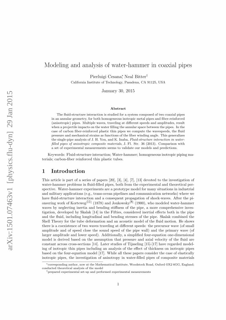
Figure 1: Schematic representation of coaxial thin pipes. LEFT: cross section. RIGHT:lateral view. Notice that here we are referring to the case of CFRP pipes with windingangles ±θ.
2 Thin pipes modeling
2.1 One-dimensional fluid-structure modeling
According to the technique of Tijsseling [17], one-dimensional governing equations for theliquid and the pipes can be obtained upon averaging out the standard balance laws in theradial direction. By adopting a cylindrical coordinates system, this approach is based uponthe assumption that the behavior of water velocity and pressure depend only on the spatial
2
Table 1: Notation. Here and in what follows subscript i is either set to be equal to 1 (in thecase in which we refer to the internal pipe) or 2 (external pipe).
Ci stiffness matrix (x,y and z coor-dinates)
ui,r, ui,z two-dimensional displacement com-ponents of pipe i along r and z axis
SSi compliance matrix (x,y and zcoordinates)
ui,r, ui,z two-dimensional velocity compo-nents of pipe i along r and z axis
r, ϕ, z cylindrical coordinates ui,r, ui,z one-dimensional velocity compo-nents of pipe i along r and z axis
t time ui,z0 magnitude of ui,zVf volume fraction (fiber) θ fiber winding anglep(r, z, t) two-dimensional fluid pressure V one-dimensional axial fluid velocityP (z, t) one-dimensional fluid pressure V0 magnitude of VP0 magnitude of P vr, vz two-dimensional fluid velocity com-
ponents along r and z directionsPout pressure outside pipe 2 εi, γi normal and shear strain in pipe iPin pressure inside pipe 1Ri inner radius of pipe i c wavespeedei thickness of pipe i σi, τi normal and shear stressρi,t density (pipe i) σi,r, σi,ϕ, σi,z two-dimensional stress components
along r, ϕ and z axisρw density of fluid σi,z one-dimensional axial stressK bulk modulus of fluid σi,z0 magnitude of σi,zE(1), E(3) effective Young’s modulus along
transverse and longitudinal di-rections in a single ply
Em, Ef Young’s modulus for matrix andfiber
G31 effective shear modulus in a sin-gle ply
Gm, Gf shear modulus for matrix and fiber
νm, νf Poisson’s ratio for matrix andfiber
ρm, ρf density of matrix and fiber
variable z. In what follows we define one-dimensional cross-averaged quantities and obtainthe corresponding field equations.
2.1.1 Governing equations for the fluid
The balance laws in the coordinate system (r, z) for the fluid read [15]
(2-d) Axial motion equation: ρw∂vz∂t
+∂p
∂z= 0,
(2-d) Radial motion equation: ρw∂vr∂t
+∂p
∂r= 0,
(2-d) Continuity equation:1
K
∂p
∂t+∂vz∂z
+1
r
∂(rvr)
∂r= 0.
Here vz(r, z, t) and vr(r, z, t) are, respectively, the axial and radial velocity of the fluid andp(r, z, t) is the pressure; K is the bulk modulus of the fluid and ρw is the density of thefluid. We now introduce the cross-sectional averaged (one-dimensional) velocity and pressure,
3
defined respectively as
V (z, t) :=1
π(R2
2 − (R1 + e1)2) ∫ R2
R1+e1
2πr vz(r, z, t)dr, (2.1)
P (z, t) :=1
π(R2
2 − (R1 + e1)2) ∫ R2
R1+e1
2πr p(r, z, t)dr. (2.2)
We are in a position to introduce the one-dimensional equations of balance for the fluid,which are
(1-d) Axial motion equation
ρw∂V
∂t+∂P
∂z= 0 (2.3)
(1-d) Radial motion equation
1
2ρwR2
∂vrdt
∣∣∣r=R2
+R2
2p∣∣∣r=R2
−(R1 + e1)2p∣∣∣r=R1+e1(
R22 − (R1 + e1)2
) − P = 0 (2.4)
(1-d) Continuity equation
1
K
∂P
∂t+∂V
∂z+
2
(R22 − (R1 + e1)2)
[R2 vr
∣∣r=R2
− (R1 + e1) vr∣∣r=R1+e1
]= 0. (2.5)
We remark that Eq. (2.4) has been obtained by multiplying the two-dimensional radialmotion equation by 2πr2, integrating in r from R1 + e1 to R2 and dividing by 2π(R2
2− (R1 +e1)2). Here R1 is the internal radius and e1 the thickness of the internal pipe while R2 is theinternal radius and e2 the thickness of the external pipe (see Fig 1-LEFT). Moreover, in Eq.(2.4) it is assumed that
r∂vrdt
= R2∂vrdt
∣∣∣r=R2
= (R1 + e1)∂vrdt
∣∣∣r=R1+e1
. (2.6)
This is consistent with the (2-d) Continuity equation under the hypothesis that K is largeand that the axial inflow vz is concentrated in the central axis in the limit R1 → 0, e1/R1 → 0[17].
2.1.2 Governing equations for the pipes
Letting i = 1, 2, the equations of Axial motion and Radial motion in the pipes in the space(r, z) are
(2-d) Axial motion equation: ρi,t∂ui,z∂t− ∂σi,z
∂z= 0,
(2-d) Radial motion equation: ρi,t∂ui,t∂t
=1
r
∂(rσi,r)
∂r− σi,ϕ
r.
Here ρi,t is the density of the pipe, σi,r(r, z, t), σi,z(r, z, t) and σi,ϕ(r, z, t) are the radial, axialand hoop stress respectively and ui,r, ui,z are the radial and axial velocity respectively. Byapplying the cross-sectional average technique we obtain
4
(1-d) Axial motion equation
ρi,t∂ui,z∂t− ∂σi,z
∂z= 0, (2.7)
(1-d) Radial motion equation
ρi,t∂ui,r∂t
=(Ri + ei)σi,r
∣∣∣Ri+ei
ei(Ri + ei/2)−
Riσi,r
∣∣∣Ri
ei(Ri + ei/2)− 1
(Ri + ei/2)σi,ϕ, (2.8)
where
ui,z(z, t) :=1
π((Ri + ei)2 −R2
i
) ∫ Ri+ei
Ri
2πr ui,z(r, z, t)dr, (2.9)
ui,r(z, t) :=1
π((Ri + ei)2 −R2
i
) ∫ Ri+ei
Ri
2πr ui,r(r, z, t)dr, (2.10)
σi,z(z, t) :=1
π((Ri + ei)2 −R2
i
) ∫ Ri+ei
Ri
2πr σi,z(r, z, t)dr, (2.11)
are respectively the one-dimensional axial velocity, radial velocity and axial stress and
σi,ϕ :=1
ei
∫ Ri+ei
Ri
σi,ϕ(r, z, t)dr. (2.12)
2.1.3 Elastic properties of pipes
By introducing the stiffness matrix Ci and the compliance matrix SSi := C−1i , the stress-
strain relation under the plane stress assumption reads, respectively, [20, Eqs. (13, 14)] σi,xσi,zτi,zx
=
Ci,11 Ci,13 0Ci,13 Ci,33 0
0 0 Ci,55
εi,xεi,zγi,zx
, (2.13)
εi,xεi,zγi,zx
=
Si,11 Si,13 0Si,13 Si,33 0
0 0 Si,55
σi,xσi,zτi,zx
.
In the case of elastically homogenous and isotropic pipes, tensor Ci reads Ci,11 Ci,13 0Ci,13 Ci,33 0
0 0 Ci,55
≡ Ei,t/(1− ν2i,t) νi,tEi,t/(1− ν2i,t) 0
νi,tEi,t/(1− ν2i,t) Ei,t/(1− ν2i,t) 00 0 Gi,t
(2.14)
and, in turn Si,11 Si,13 0Si,13 Si,33 0
0 0 Si,55
=
1/Ei,t −νi,t/Ei,t 0−νi,t/Ei,t 1/Ei,t 0
0 0 1/Gi,t
(2.15)
5
y,2
y
z
z
3
x
+θ
−θ
−θ+θ
zy
x
x
1
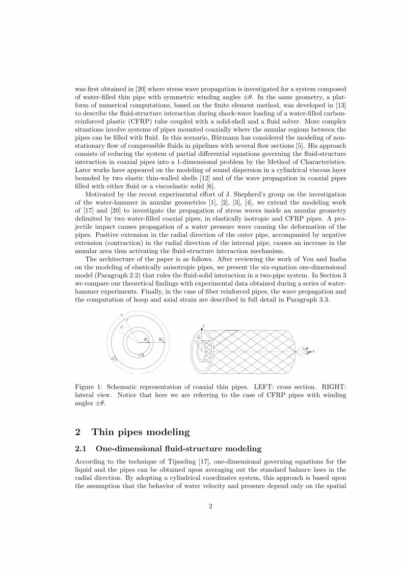
Figure 2: Schematic rep-resentation of CFRP lay-up structures as a com-bination of single uniaxialplies. Axes 1, 2 and 3 arethe principal axes of a sin-gle ply.
where Ei,t, νi,t and Gi,t = Ei,t/(2+2νi,t) are the Young’s modulus, Poisson’s ratio and shearmodulus of the material from which pipe i is made.
For anisotropic composite (fiber-reinforced) pipes the stiffness elements Ci,kl are neces-sarily a function of the geometric and elastic properties of fibers and of matrix, including thefiber winding angle θ. The difficulty in describing the elastic properties of fiber-reinforcedplastic thin pipes has been studied in [20] under the assumption that pipes are obtained byrolling up a woven layer with symmetric angles ±θ. Each of these layers can be consideredas a lay-up structure of multiple plies of same thickness as shown in Figure 2. To keep thenotation simple, in what follows we drop the subscript i. Elastic moduli are computed as afunction of fiber volume fraction Vf and fiber and matrix elastic coefficients [9]
where Em, Gm, νm and ρm are, respectively, the Young’s modulus, shear modulus, Poisson’sratio and density of the matrix. Then Ef , Gf , νf and ρf are, respectively, the fiber Young’smodulus, shear modulus, Poisson’s ratio and density of the fiber. The subscripts 3 and 1indicate the longitudinal and transverse direction of a single ply (see Fig. 2). The Poisson’sratio ν31 is defined as the ratio of the contracted normal strain in the direction 1 to the normalstrain in the direction 3, when a normal load is applied in the longitudinal direction. Thestiffness matrix for the composite is given by the volumetric average of the elastic stiffness
matrices from each single ±θ ply, denoted in what follows with C±θ
. Precisely, if all plieshave the same thickness, the stiffness matrix for a woven layer of pairs of ±θ plies is givenby
respectively. By using the strain-displacements relations
εi,z =∂ui,z∂z
, (2.20)
by differentiating in time and by taking the cross-sectional average, Eq. (2.19)-LEFT becomes
∂ui,z∂z
= Si,13∂σi,ϕ∂t
+ Si,33∂σi,z∂t
(2.21)
where
σi,ϕ(z, t) :=2π
π((Ri + ei)2 −R2
i
) ∫ Ri+ei
Ri
r σi,ϕ(r, z, t)dr (2.22)
is the one-dimensional (cross-averaged) hoop stress.The radial displacement equation is obtained by plugging another strain-displacement
relation, which is,
εi,ϕ =ui,rr
(2.23)
into Eq. (2.19)-RIGHT yielding
ui,r = rSi,11σi,ϕ + rSi,13σi,z. (2.24)
The equations of fluid and pipes are coupled by boundary conditions along the interfaces.Indeed, at each fluid-solid interface, we equate the radial velocity and radial stress of thefluid with those of the solid.
σ2,r∣∣r=R2
= −p∣∣r=R2
, u2,r∣∣r=R2
= vr∣∣r=R2
,
σ1,r∣∣r=R1+e1
= −p∣∣r=R1+e1
, u1,r∣∣r=R1+e1
= vr∣∣r=R1+e1
,
σ2,r∣∣r=R2+e2
= −P out = const., u2,r∣∣r=R2+e2
= V outr = const. (= 0m/s),
σ1,r∣∣r=R1
= −P in = const., u1,r∣∣r=R1
= V inr = const. (= 0m/s).
(2.25)
As in [17], we assume that the external and internal pressures in each pipe induce a hoopstress which is constant in ϕ. Accordingly, we have [20], [18]
σ1,ϕ = − 1
r2R2
1(R1 + e1)2(P − P in)
2(R1 + e1/2)e1+R2
1Pin − (R1 + e1)2P
2(R1 + e1/2)e1
σ2,ϕ = − 1
r2R2
2(R2 + e2)2(Pout − P )
2(R2 + e2/2)e2+R2
2P − (R2 + e2)2Pout2(R2 + e2/2)e2
.
(2.26)
7
By plugging Eqs. (2.25-Lines 1 and 2, RIGHT) into Eq. (2.5) we obtain
1
K
∂P
∂t+∂V
∂z+
2
(R22 − (R1 + e1)2)
[R2 u2,r
∣∣∣r=R2
− (R1 + e1) u1,r
∣∣∣r=(R1+e1)
]= 0. (2.27)
Now, assuming that radial inertial forces are ignored in both fluid and pipes and that the pipescross-sections remain plane for axial stretches (thus implying the independency of σi,z(z, t)on r, especially in thin pipes) we obtain a simplified model. Upon substitution of Eqs. (2.24)and (2.26) into Eq. (2.27) and upon substitution of Eq. (2.26) into (2.21) (by replacingσ1,z
∣∣r=R1+e1
= σ1,z, σ2,z∣∣r=R2
= σ2,z) we obtain new equations
m21∂P
∂t+∂V
∂z+m24
∂σ2,z
∂t−m23
∂σ1,z
∂t= 0, (2.28)
and
∂u1,z∂z
= m51∂P
∂t+ S1,33
∂σ1,z
∂t,
∂u2,z∂z
= m61∂P
∂t+ S2,33
∂σ2,z
∂t(2.29)
where
m21 :=1
K+
2{R2
2
[S2,11
(R2 + e2)2 +R22
2(R2 + e2/2)e2
]+ (R1 + e1)2
[S1,11
R21 + (R1 + e1)2
2(R1 + e1/2)e1
]}(R2
2 − (R1 + e1)2)
≈ 1
K+
2
R22 − (R1 + e1)2
[S2,11
R32
e2+ S1,11
(R1 + e1)3
e1
]m23 := S1,13
2(R1 + e1)2
R22 − (R1 + e1)2
m24 := S2,132R2
2
R22 − (R1 + e1)2
m51 := S1,13H1
m61 := S2,13H2
(2.30)
with
H1 := − ln(
1 +e1R1
)[ (R1 + e1)2
2(R1 + e1/2)e1
] 2R21
e1(2R1 + e1)− (R1 + e1)2
2(R1 + e1/2)e1≈ −
(R1 + e1e1
)H2 := ln
(1 +
e2R2
)[ (R2 + e2)2
2(R2 + e2/2)e2
] 2R22
e2(2R2 + e2)+
R22
2(R2 + e2/2)e2≈ R2
e2.
(2.31)
The simplified expressions in Eqs. (2.30) and (2.31) are obtained under the assumption(e1/(R1 + e1)) � 1, e2/R2 � 1. Note that it is not possible for the terms in Eq. ((2.30) tobecome singular, since the denominator becomes zero only when the annulus of water haszero thickness. Summarizing, the six-equations model with the six unknowns(P, V, σi,z, ui,z)for the two-pipe system read
Fluid (axial motion - continuity equation)
ρw∂Vz∂t
+∂P
∂z= 0, (2.32)
m21∂P
∂t+∂V
∂z+m24
∂σ2,z
∂t−m23
∂σ1,z
∂t= 0, (2.33)
8
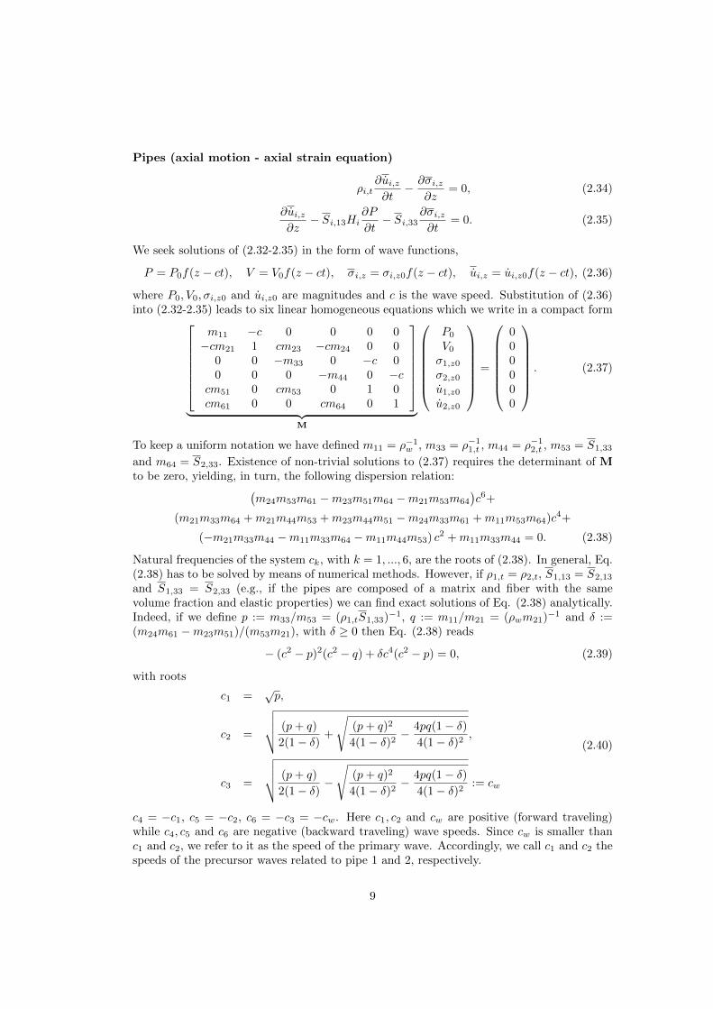
Pipes (axial motion - axial strain equation)
ρi,t∂ui,z∂t− ∂σi,z
∂z= 0, (2.34)
∂ui,z∂z− Si,13Hi
∂P
∂t− Si,33
∂σi,z∂t
= 0. (2.35)
We seek solutions of (2.32-2.35) in the form of wave functions,
where P0, V0, σi,z0 and ui,z0 are magnitudes and c is the wave speed. Substitution of (2.36)into (2.32-2.35) leads to six linear homogeneous equations which we write in a compact form
m11 −c 0 0 0 0−cm21 1 cm23 −cm24 0 0
0 0 −m33 0 −c 00 0 0 −m44 0 −c
cm51 0 cm53 0 1 0cm61 0 0 cm64 0 1
︸ ︷︷ ︸
M
P0
V0σ1,z0σ2,z0u1,z0u2,z0
=
000000
. (2.37)
To keep a uniform notation we have defined m11 = ρ−1w , m33 = ρ−11,t , m44 = ρ−12,t , m53 = S1,33
and m64 = S2,33. Existence of non-trivial solutions to (2.37) requires the determinant of Mto be zero, yielding, in turn, the following dispersion relation:(
Natural frequencies of the system ck, with k = 1, ..., 6, are the roots of (2.38). In general, Eq.(2.38) has to be solved by means of numerical methods. However, if ρ1,t = ρ2,t, S1,13 = S2,13
and S1,33 = S2,33 (e.g., if the pipes are composed of a matrix and fiber with the samevolume fraction and elastic properties) we can find exact solutions of Eq. (2.38) analytically.Indeed, if we define p := m33/m53 = (ρ1,tS1,33)−1, q := m11/m21 = (ρwm21)−1 and δ :=(m24m61 −m23m51)/(m53m21), with δ ≥ 0 then Eq. (2.38) reads
− (c2 − p)2(c2 − q) + δc4(c2 − p) = 0, (2.39)
with roots
c1 =√p,
c2 =
√√√√ (p+ q)
2(1− δ) +
√(p+ q)2
4(1− δ)2 −4pq(1− δ)4(1− δ)2 ,
c3 =
√√√√ (p+ q)
2(1− δ) −√
(p+ q)2
4(1− δ)2 −4pq(1− δ)4(1− δ)2 := cw
(2.40)
c4 = −c1, c5 = −c2, c6 = −c3 = −cw. Here c1, c2 and cw are positive (forward traveling)while c4, c5 and c6 are negative (backward traveling) wave speeds. Since cw is smaller thanc1 and c2, we refer to it as the speed of the primary wave. Accordingly, we call c1 and c2 thespeeds of the precursor waves related to pipe 1 and 2, respectively.
9
2.2.1 Reconstruction of the physical quantities
We are now able to recover the mechanical strain in the hoop and axial directions as functionsof P, V, σi,z, ui,z. Thanks to Eq. (2.19)-RIGHT we can write the one-dimensional hoop strainas follows
εi,hoop = εi,ϕ =1
2π(Ri + ei/2)ei
∫ Ri+ei
Ri
2πr εi,ϕdr = Si,11σi,ϕ + Si,13σi,z,
where σi,ϕ has been obtained in (2.26) (with Pin = Pout = 0). In turn, we have
The cross-sectional averaged axial strain can be obtained by Eqs. (2.20) and (2.35)
εi,ax = εi,z =1
2π(Ri + ei/2)ei
∫ Ri+ei
Ri
2πrεi,zdr =∂ui,z∂z
= − ui,z0c
f(z − ct) =
Si,13HiP0f(z − ct) + Si,33σi,z0f(z − ct). (2.42)
Notice that here ui,z = (−ui,z0/c)F (z − ct) follows from integrating the last equation in(2.36) over time with F ′ = f . Then, from the system of equations (2.37) we can easily derivethe following relations
ui,z0 =cSi,13HiP0
(−1 + c2Si,33ρi,t), σi,z0 = −cρi,t
cSi,13HiP0
(−1 + c2Si,33ρi,t), (2.43)
and, by taking c = c3 = cw,
P0 = cwρwV0. (2.44)
Thanks to Eq. (2.44) we can express averaged hoop and axial stress dependent on either thefluid velocity V0 or, upon inversion of Eq. (2.44), on the fluid pressure P0. By plugging Eqs.(2.43)-RIGHT and (2.44) into Eq. (2.41) and (2.42) with c = cw we obtain
εi,hoop ={Si,11Hi + Si,13
[−cwρi,t
cwSi,13Hi
(−1 + c2wSi,33ρi,t)
]}cwρwV0f(z − cwt), (2.45)
εi,ax = − Si,13Hi
(−1 + c2wSi,33ρi,t)cwρwV0f(z − cwt), (2.46)
σi,z0 = −ρi,tc2wSi,13Hi
(−1 + c2wSi,33ρi,t)cwρwV0.
3 Water-hammer experiments
Armed with the set of analytic expressions from Section 2, we turn now to the simulationof experimental measurements for the water-hammer experiment for a set of pipes includinghomogeneous (isotropic) metal pipes and fiber-reinforced (anisotropic) pipes.
3.1 Experimental setup
The propagation of waves in the annular space between two pipes is studied experimentallyusing the apparatus shown in Fig. 3. For all experiments, the outer pipe is a thick-walled
10
Pressure Transducer Ports
(6 total)
Electrical
Feed-through
Confining
Outer Tube Specimen
Tube
Support Plate
Buffer Projectile from
gas gun
Internal plug with
gland seals
Water
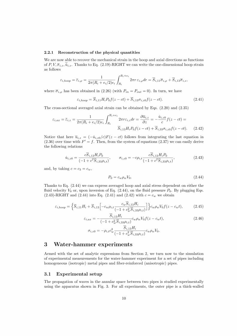
Figure 3: Diagram of apparatus used to measure wave propagation speeds (rotated 90◦
counterclockwise). “Electrical feedthrough” provides a sealed connection between the leadsof strain gauges (attached to specimen tube) and the data acquisition electronics external tothe setup. The web version of this article contains the above plot figure in color.
cylindrical vessel made from 4140 high strength steel with an inner radius R2 = 38.1 mm,wall thickness e2 = 25.4 mm, and length 0.97 m. Tubes of various sizes can be mountedconcentrically inside of this vessel; these tubes are held in place at both ends by polycarbonateplugs and sealed with gland seals. The plug at the right end of Fig. 3 is fixed to the baseof the setup while the plug at the left end is fixed to a “support plate” (Fig. 3 inset) whichfeatures four holes that allow pressure waves to pass freely while still providing support forthe inner tube.
The annular space between the two pipes is filled with distilled water while the sealedcavity inside of the inner pipe remains filled with air at ambient pressure. The water insidethe annular cavity is also at atmospheric pressure at the beginning of the test. An aluminum“buffer” is then inserted into the top of the apparatus, and any air that remains in the systemis vented through a hole in the buffer that is later sealed. The buffer is composed of a 125 mmlong aluminum cylinder capped by a 25 mm thick steel striker plate which prevents damageof the buffer during projectile impact; this striker plate is bolted to the aluminum bufferusing eight 1/4-20 machine screws.
Next a projectile is fired from a gas gun into the buffer, and the stress wave that develops inthe buffer is transmitted into the water as a shock wave which travels along the annular spacebetween the inner and outer pipes. Examples of pressure traces plotted on an x− t diagramare shown in Fig. 4; they demonstrate a sharp shock wave followed by an approximatelyexponential decay. Slight steepening of the wavefront is visible as the wave progresses. Thehigh frequency fluctuations in the pressure signal are the result of axisymmetric vibrationsof the inner pipe, as was confirmed by hoop strain measurements (not shown) at multiplelocations around the circumference.
The axial propagation speed of the pressure wave is measured using a row of six pressuretransducers, PCB model 113A23, which have a response time less than 1 µs, resonant fre-quency above 500 kHz, and are sampled at 1 MHz. These transducers are mounted flush withthe inner surface of the outer pipe. The response of the tube is recorded using bonded straingauges oriented in the hoop direction, which are coated with a compliant sealant (VishayPG, M-Coat D) to avoid electrical interference from the water. Signals are amplified usingVishay 2310B signal conditioners and digitized at 1 MHz.
The speed of the pressure wave is measured by marking the time of arrival of the pressurewave at each transducer and fitting a line to the data as shown in Fig. 4; the slope of this lineis the wave speed. The time of arrival of the pressure wave at each transducer is determined
11
−1 0 1 2 3 4 50.3
0.4
0.5
0.6
0.7
0.8
0.9
1
Time [ms]
Dis
tance F
rom
Reflecting E
nd [
m]
Tube 42; Shot 237; Pressure
15
20
25
30
35
40
45
Pre
ssure
[M
Pa]
Reflected WaveIncident Wave
Figure 4: Example of experimental pressure traces used to determine wave propagation speed.
as the first instant at which the pressure exceeds a chosen threshold. Because the shock wavesteepens as it progresses, the wave speed depends slightly on chosen threshold level. For theresults reported in this paper, wave speeds were calculated using both 50% and 80% of themaximum pressure of the incident wave as threshold values, and in every case the resultsdiffered by less than 5%. The lower threshold value of 50% was chosen because it is largerthan the amplitude of the precursor wave, which ensures that the measured primary wavespeed is not influenced by that of the precursor wave.
For each specimen tube, between 3 and 8 shots were conducted. After each shot, wavespeeds were calculated using both 50% and 80% of the maximum pressure as the thresholddescribed above, and the average of these two values was taken as the measured wave speedfor the shot. Finally, the average wave speed over all 3-8 shots was calculated, and thisnumber was taken to be the wave speed associated with the specimen. The uncertainty inthe measured wave speed was calculated as twice the standard deviation of the measuredwave speeds over all 3-8 shots; this uncertainty is typically less than 10%. The difference inmeasured wave speed between shots depends mainly on the quality of the impact between theprojectile and buffer. Slight non-normal impact is unavoidable and leads to slight differencesin the measured velocity.
Further details about the experimental setup are recorded in Refs. [3, 4]. It may be notedthat the experiment was designed for the study of plastic deformation and buckling of tubesloaded by dynamic external pressure, which is the reason for the rather high pressure of theshock wave (on the order of 1-10 MPa). For all results reported in this paper, the pressureand total impulse of the pressure load were low enough to prevent plastic deformation of boththe inner and outer pipes, as was verified by hoop strain measurements. Although the hoopstrain measurements indicated slight non-axisymmetric deformation of the inner pipe (elasticbuckling) in most shots, these effects do not appear to significantly influence the propagationof pressure waves so long as the buckles remain elastic (see Ref. [3]).
12
Table 2: Parameters of the large 4140 steel tube (referred as pipe 2 in Section 3) and water.4140 Steel (pipe 2)Young’s modulus E2,t 198 GPa Inner radius R2 38.1 mmDensity ρ2,t 7800 kg/m3 Thickness e2 25.4 mmPoisson’s ratio ν2,t 0.3WaterBulk modulus K 2.14 GPaDensity ρw 999 kg/m3
Table 3: Parameters of stainless steel and aluminum.Aluminum (pipe 1) Stainless steel (pipe 1)Young’s modulus E1,t 68.9 GPa Young’s modulus E1,t 198 GPaDensity ρ1,t 2700 kg/m3 Density ρ1,t 8040 kg/m3
Poisson’s ratio ν1,t 0.33 Poisson’s ratio ν1,t 0.29
3.2 Results and discussion
We now address our experimental measurements of the speed of the primary wave, the fluidpressure and the hoop strain in the internal pipe against the prediction based on our modelingwork. The geometrical and physical properties of the external pipe are reported in Table 2.The smaller interior tubes are mounted concentrically and are made from either aluminum,stainless steel (with properties listed in Tables 3 and 4) or a carbon fiber-epoxy resin matrixcomposite. The elastic coefficients matrices Ci and SSi for both the internal (i = 1) andexternal (i = 2) pipe are computed as in Paragraph 2.1.3 with the only exception being theCFRP pipe for which a clarification of the method is given in the Remark below. Noticethat since the physical properties of the external and internal pipes are different, and inparticular C1 6= C2, computation of the primary wave speed cw needs to be accomplishedby solving Eq. (2.38) numerically. Results displayed in Table 4 show a good match betweenthe experimental data and the predicted values. However, there are some slight differences;in particular, the measured wave speeds are consistently greater than those predicted by themodel. One possible explanation is that the steepening wavefront of the pressure wave biasesthe experimental measurements toward higher wave speeds.
Comparisons of experimental measurements and predictions for hoop and axial strain inthe internal pipe, given in Table 5, show that the calculated data match with experimentalresults reasonably well. In this table the measured data points are the peak values of thepressure and hoop strain, which were determined after applying a 50 kHz low-pass filter to therecorded signals. The computed values of these physical variables are based on cw since theprimary wave generates larger magnitudes in both axial and hoop strain than the precursorwaves. Differences between the computed and measured values are the result of modelingidealizations that are not completely satisfied in the experiment. For instance, radial inertiaof the fluid and pipes, strain rate effects, axial bending of the pipe in the vicinity of thewavefront, non-planar features of the pressure wavefront, and transient phenomena, maywell contribute to the differences between measurement and computation.
Although only direct measurements for the fluid pressure are available, we are able toreport estimated data for the fluid velocity as well. Since a direct measurement of the fluidvelocity is not available, the fluid velocity behind the wavefront is estimated as being equalto the initial velocity of the buffer (see Fig. 3). The initial buffer velocity was estimatedby equating the momentum of the projectile prior to impact with that of the buffer after
13
impact. In other experiments using the same experimental setup, high speed video of theprojectile-buffer impact has shown that this estimate of the buffer velocity is typically within10-20% of its actual velocity.
Table 4: Geometrical parameters of pipe 1 (six different cases). † = aluminum, ‡ = stainlesssteel, ? = carbon-epoxy composite.
Speed of primary wave cw [m/s]Tube ID R1 [m] e1 [mm] Measurement Computation
Table 5: Comparison of measurements and predictions of maximum hoop strain accompa-nying the water-hammer wave (pipe 1) and fluid velocity. Here the fluid velocity V †0 was notmeasured, but instead was estimated at the post-processing level. Variables with a super-script ] have been computed using the water pressure P0 determined from the experimentsand by using Eqs. (2.44) and (2.45).
Experiments Computations
Shoot ID P0 ε1,hoop V †0 ε]1,hoop V ]0[MPa] [mstr] [m/s] [mstr] [m/s]
100 (tube ID 27) 3.10 -0.61 2.86 -0.6581 2.57106 (tube ID 27) 6.44 -1.23 5.69 -1.3672 5.34137 (tube ID 34) 2.64 -0.93 2.83 -0.9816 2.51151 (tube ID 35) 4.98 -1.37 3.97 -1.3325 3.89200 (tube ID 38) 3.05 -0.55 3.14 -0.8161 2.38159 (tube ID 36) 7.92 -0.61 5.22 -0.7054 5.76160 (tube ID 36) 11.10 -0.76 6.19 -0.9886 8.07398 (tube ID 40) 3.12 -1.56 - -1.3 -
Remark 1. While our analysis is valid for pipes of various thicknesses and elastic moduli,experimental results are available only for a system where thin internal pipes are coupled toa relatively thick and stiff outer pipe. In this regime, the external pipe is almost rigid and themain contributions to the fluid-structure interaction are due to the internal pipe. To clarifythis point, we analyze the dependence of the primary wave speed on certain parameters ofthe external pipe. As an example, we limit our analysis to systems with an internal pipemade of stainless steel with parameters reported in Table 3. Similar results can be obtainedby considering an aluminum or composite pipe.
In Fig. 6-LEFT we report the computation of the primary wave speed as a functionof the thickness of the external pipe and considering the Young’s modulus of pipe 2 as aparameter. Therefore the continuous curve corresponds to 4140 steel while the other curvescorrespond to a material with increasing stiffness including the limit case of an ideally rigidmaterial. Interestingly, the computed value of the primary wave speed for a 4140 steel pipewith internal radius R1 = 38.1 mm and thickness of e1 = 25.4 mm (cw = 1369 m/s, Table 4)
14
0.01 0.015 0.02 0.025 0.03
800
1100
1400
R1 [m]
[m/s
]
computed
experiment (ID 36)
computed
experiment (ID 35)
experiment (ID 34)
0.01 0.015 0.02 0.025 0.03
800
1100
1400
R1 [m]
[m/s
]
computed
experiment (ID 27)
computed
experiment (ID 40)
computed
experiment (ID 38)
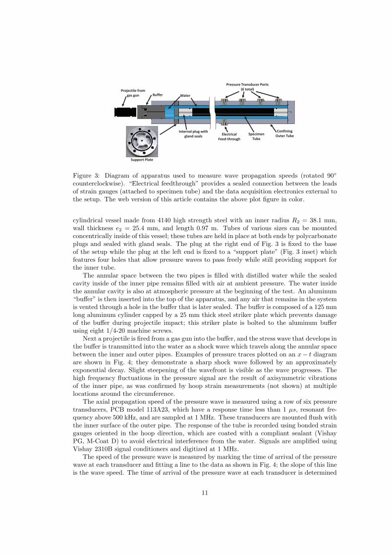
Figure 5: Comparison of computed primary wave speed cw and experimental measurements.LEFT: aluminum, tube IDs 34 and 35 (prediction reported as continuous line); stainless steel,tube ID 36 (prediction reported as dashed line). RIGHT: carbon-epoxy composite, tube ID40 (prediction reported as a continuous line); aluminum, tube ID 27 (prediction reported asdashed line) and ID 38 (dash-dotted line). The web version of this article contains the aboveplot figures in color.
0.005 0.01 0.015 0.02 0.025 0.03900
1000
1100
1200
1300
1400
e2 [m]
[m/s
]
computed, E2t
=1 x 198 GPa
computed, E2t
=2 x 198 GPa
computed, E2t
=3 x 198 GPa
computed, E2t
= ∞ GPa
experiment (ID 36)
0.01 0.015 0.02 0.025 0.03
800
1000
1200
1400
R1 [m]
[m/s
]
computed, e2=25.4 mm
computed, e2=5.08 mm
computed, e2=2.54 mm
experiment (ID 36)
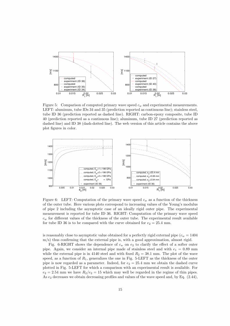
Figure 6: LEFT: Computation of the primary wave speed cw as a function of the thicknessof the outer tube. Here various plots correspond to increasing values of the Young’s modulusof pipe 2 including the asymptotic case of an ideally rigid outer pipe. The experimentalmeasurement is reported for tube ID 36. RIGHT: Computation of the primary wave speedcw for different values of the thickness of the outer tube. The experimental result availablefor tube ID 36 is to be compared with the curve obtained for e2 = 25.4 mm.
is reasonably close to asymptotic value obtained for a perfectly rigid external pipe (cw = 1404m/s) thus confirming that the external pipe is, with a good approximation, almost rigid.
Fig. 6-RIGHT shows the dependence of cw on e2 to clarify the effect of a softer outerpipe. Again, we consider an internal pipe made of stainless steel and with e1 = 0.89 mmwhile the external pipe is in 4140 steel and with fixed R2 = 38.1 mm. The plot of the wavespeed, as a function of R1, generalizes the one in Fig. 5-LEFT as the thickness of the outerpipe is now regarded as a parameter. Indeed, for e2 = 25.4 mm we obtain the dashed curveplotted in Fig. 5-LEFT for which a comparison with an experimental result is available. Fore2 = 2.54 mm we have R2/e2 = 15 which may well be regarded in the regime of thin pipes.As e2 decreases we obtain decreasing profiles and values of the wave speed and, by Eq. (2.44),
15
of the fluid pressure as well. Indeed, softer pipes undergo large radial deformations causingan increase of the annular area and consequently a drop of pressure.
Remark 2. The computations of the elastic stiffness for carbon-epoxy composite tubesdeserves a special comment. When we have more fibers in one direction than in another wemust adapt the method used in Paragraph 2.1.3. Indeed, since tube 40 is a lay-up structure oflayers containing fibers in both axial (θ = 0o) and transverse (θ = 90o) direction, its stiffnessmatrix, denoted by C
ce
1 , is determined by a volumetric average of the two stiffness matrices
obtained by plugging θ = 0o or θ = 90o into C+θ
. Although the exact proportion of plies withfibers in either direction is unknown, we have been able to estimate the elastic coefficients
by simply assuming that the known coefficient Cce
1,33 is given by a linear combination of C0o
33
and C90o
33 [10]. Indeed, by solving the system of equations
Cce
1,11 = ξ C0o
11 + (1− ξ)C90o
11 , Cce
1,33 = ξ C0o
33 + (1− ξ)C90o
33 , (3.1)
we are able to compute the two unknown variables Cce
1,11 and ξ. The latter, ξ, is the relativeamount of fibers in the axial direction, a non-dimensional parameter which takes into accountboth the percentage of plies with fibers in the axial direction and their thickness. For pipescomposed of uniaxial layers with all fibers in direction θ = 0o we have ξ = 1, while in thedual case of fiber-reinforced pipes with winding angle θ = 90o we have ξ = 0. Notice that theelastic coefficient for CFRP pipes in Paragraph 2.1.3 have been computed for ξ = 0.5 since wehave the same amount of plies with winding angle +θ as those with winding angle −θ and all
the plies have the same thickness. By plugging C0o
33 = C90o
11 = 142 GPa and C0o
11 = C90o
33 = 9GPa [24] and C
ce
1,33 = 117 GPa [23] yields Cce
1,11 ≈ 34 GPa and ξ ≈ 0.8. Finally, the compu-tation of the density of the composite and of the Poisson’s ratio follow as in Eq. (2.17) by
resin) [20] with fiber volume fraction Vf = 2/3 [23] yielding ν31 = 0.26 and ρ1,t = 1583 kg/m3.
Investigation of the pressure waves and mechanical strain profiles becomes particularlytransparent when the system is composed of two coaxial carbon-reinforced pipes and whenfibers and matrix have the same physical properties in both pipes. Even though for this caseexperimental results are not available, in the following we report the analysis for the readersconvenience thus generalizing the one-pipe modeling work of [20].
3.3 Fiber-reinforced plastic pipes
The study of the fluid-structure interaction in anisotropic structures, considered for the firsttime in this paper with the modeling tube ID 40 in Paragraph 3.2, is now analyzed in fulldetail for a system of two coaxial water-filled CFRP pipes composed of pairs of ±θ pliesof same thickness. To keep our analysis simpler, we assume that the physical properties ofmatrix and fibers (including the winding angle) are identical to one another in both pipes (seeTable 6) yielding C1,kl = C2,kl. As in Paragraph 2.1.3 we drop the subscript i in the stiffnessand compliance coefficients. The general case of pipes with different properties, includingdifferent winding angles θ1 6= θ2, can be studied with similar techniques and is left to thebrave reader.
The plots of the stiffness and compliance elements Ckl and Skl as a function of the windingangle θ are contained in [20]. Here it is enough to recall that at θ = 0◦, the direction of thefibers coincides with the axial direction of the pipes and consequently the axial stiffness C33
has a maximum while the hoop stiffness C11 has a minimum. As θ increases, C11 increases
16
while C33 decreases due to the fiber reinforcement in the hoop direction. Conversely, as θincreases, S11 decreases while S33 increases. Then, the absolute values of the coupling termsC13 and S13 have a maximum at θ = 45o and are minimized at θ = 0o and 90o.
Table 6: Geometrical and physical data for coaxial CFRP pipes, [20].Carbon fiber Epoxy resin (matrix)Young’s modulus Ef 238 GPa Young’s modulus Em 2.83 GPaDensity ρf 1770 kg/m3 Density ρm 1208 kg/m3
Poisson’s ratio νf 0.2 Poisson’s ratio νm 0.39Composite pipesInner radius (pipe 1) R1 19.15 mm Inner radius (pipe 2) R2 54 mmThickness (pipe 1, 2) e1=e2 1.66 mm Fiber volume fraction Vf 0.7
The calculated primary and precursor waves are shown in Fig. 7 as functions of θ. Similar tothe one-pipe scenario of [20], as θ increases the result is a reinforcement of the hoop stiffnessand an increase in the primary wave speed which corresponds to the breathing mode of thepipes. Conversely, the speed of the precursor waves (corresponding to a longitudinal modeof the pipes) diminishes due to decreased axial stiffness. We remark that the computationof the physical variables is based on the incident wave c = cw because its magnitude is muchlarger than those of precursor waves. In this case, by Eq. (2.44) we have P0/V0 = cwρw andtherefore the graph of the fluid pressure is not reported. Precursor wave speeds c1 and c2are very similar when the parameter δ is very small which happens for either small or largeθ. This is consistent with Eq. (2.40) where for δ = 0 we have c1 = c2. It is possible toprove that this corresponds to the cases for which the coupling stiffness S13 as a function ofθ is minimal. On the other hand, it follows that for intermediate values of θ wavespeed c1becomes slower while δ becomes larger and is maximized at θ ≈ 43o when also S13 is large.Proof of the dependence of δ on the coupling term S13 requires a more detailed asymptoticanalysis and it is therefore left to a forthcoming paper. Plots of the hoop and axial strainin pipes 1 and 2 calculated from Eqs. (2.45) and (2.46) are reported in Fig. 8. As theimpulsive impact by the projectile generates a positive water pressure, pipe 2 undergoes apositive expansion in the radial direction (hoop strain is positive) while pipe 1 is contractedin the radial direction (hoop strain is negative). Note that the radial expansion of pipe2 accompanies the contraction in the axial direction while the radial contraction of pipe 1accompanies the expansion in the axial direction. This explains why hoop and axial strainhave opposite signs. The hoop strain is essentially determined by the hoop compliance S11
and therefore the absolute values of the hoop strains in both pipe 1 and 2 are large for smallθ and are decreasing for increasing θ. Then, at a first order of approximation, the axial strainis mainly determined by the coupling term S13 [20, Sect. 5] and therefore the axial strainsin both pipe 1 and 2 are maximized (in absolute value) for θ ≈ 52o.
4 Summary and future perspectives
We have investigated the propagation of stress waves in water-filled pipes in an annular ge-ometry. A six-equation model that describes the fluid-structure interaction has been derivedand adapted to both elastically isotropic and anisotropic (fiber-reinforced) pipes. The nat-ural frequencies of the system (eigenvalues) and the amplitude of the pressure and velocityof the fluid, along with the mechanical strains and stresses in the pipes (eigenvectors) havebeen computed and compared with experimental data of water-hammer tests. It is observed
17
0 20 40 60 80
400
600
800
1000
θ [deg]
[m/s
]
0 20 40 60 80
2000
4000
6000
8000
10000
θ [deg]
c1 [m/s]
c2 [m/s]
2000 x δ
Figure 7: LEFT: plot of the primary wave speed cw, RIGHT: plot of the precursor wavespeeds c1 and c2 as a function of the winding angle θ and of the coefficient δ (non-dimensional,multiplied by 2000) as a function of θ. The web version of this article contains the aboveplot figure in color.
0 20 40 60 80−5
0
5
10
x 10−4
θ [deg]
[str
/(m
/s)]
Hoop strain
pipe 1
pipe 2
0 20 40 60 80−10
−5
0
x 10−4
θ [deg]
[str
/(m
/s)]
pipe 1
pipe 2
Axial strain
Figure 8: LEFT: plot of the maximum hoop strains accompanying the water-hammer wavenormalized by V0 = 1 m/s as a function of the winding angle θ (Eqs. (2.45)). RIGHT: plotof the maximum axial strains accompanying the water-hammer wave normalized by V0 = 1m/s as a function of the winding angle θ (Eq. (2.46)).
that the projectile impact causes a positive expansion of the external pipe in the radial di-rection and a contraction in the axial direction (Poisson’s effect). Vice versa, the internalpipe is contracted in the radial direction and expanded axially. In the last section of thepaper, which is a benchmark for future experimental investigation, we have analyzed in fulldetail the propagation of waves in CFRP pipes with a special emphasis on the influence ofthe winding angle on the wave speeds and the axial and hoop strains in the pipes. Mostinterestingly, we found that the speed of the primary wave (breathing mode) increases withthe increasing winding angle due to increasing hoop stiffness in both pipes. This is in agree-ment with the one-pipe model and analysis of [20]. Conversely, the profile of the speed of theprecursor waves (longitudinal modes) is large when the winding angle is small (and thereforethe axial stiffness is large) and it decreases with increasing winding angle. Additionally, wehave observed that the two precursor waves travel at almost the same speed when the fiberwinding angle is equal to either 0o or 90o while a separation of the velocities is observed forθ in between these values, a phenomenon which is the object of further analysis.
18
Acknowledgments
The authors are indebted to Prof. K. Bhattacharya and J. Shepherd for many useful discus-sions and their advice. P.C. acknowledges support from the Department of Energy NationalNuclear Security Administration under Award Number DE-FC52-08NA28613. This workwas written when P.C. was a postdoctoral student at the California Institute of Technology.
References
[1] Beltman, W., Burscu, E., Shepherd, J., Zuhal, L., 1999. The Structural Response ofCylindrical Shells to Internal Shock Loading. ASME J. Pressure Vessel Technol., 121(3).
[2] Beltman, W., Shepherd, J., 2002. Linear Elastic Response of Tubes to Internal Detona-tion Loading. J. Sound Vib., 252(4).
[3] Bitter, N., Shepherd, J., 2013. Dynamic buckling and fluid-structure interaction of sub-merged tubular structures, in: Blast mitigation: experimental and numerical studies,Editors A. Shukla, Y. Rajapakse, and M.E. Hynes, Springer.
[4] Bitter, N., Shepherd, J., 2013. Dynamic buckling of submerged tubes due to impul-sive external pressure, Proceedings of 2013 SEM annual conference and exposition onexperimental and applied mechanics, June 3-5, 2013, Lombard, IL.
[5] Burmann, W., 1975. Water hammer in coaxial pipe systems. ASCE Journal of the Hy-draulics Division, Vol. 101, No. HY6, pp. 669-715.
[6] Cirovic, S., Walsh, C., Fraser, W.D., 2002. Wave propagation in a system of coaxialtubes filled with incompressible media: A model of pulse transmission in the intercranialarteries. Journal of Fluids and Structures, 16 (8), pp. 1029-1049.
[7] Inaba, K., Shepherd, J., 2008. Impact generated stress waves and coupled fluid-structureresponses, Proceedings of the (SEM) XI International congress and exposition on exper-imental and applied mechanics, June 2-5, Orlando, FL USA.
[8] Joukowsky, N., 1900. Uber den hydraulischen stoss in wasserleitungsrohren. Memoiresde l’Academie Imperiale des Sciences de St.Petersburg, series 8, p.9.
[11] Korteweg, D., 1878. Uber die fortpflanzungsgeschwindigkeit des schalles in elastischenrohren, Annalen der Physik und Chemie 9 folge 5, 525-542.
[12] Levitsky, S.P., Bergman, R.M., Haddad, J., 2004. Wave propagation in a cylindricalviscous layer between two elastic shells. International Journal of Engineering Science, 42(19-20), pp. 2079-2086.
[13] Perotti, L.E., Deiterding, R., Inaba, K., Shepherd, J., Ortiz, M., 2013. Elastic responseof water-filled fiber composite tubes under shock wave loading, International Journal ofSolids and Structures, Vol. 50, Issues 3-4.
[14] Skalak, R., 1956. An extension of the theory of water hammer, Transactions of theASME 78, 105.
19
[15] Tijsseling, A.S., 1993. Fluid-structure interaction in case of waterhammer with cavita-tion, PhD Thesis, Delft University of Technology, Faculty of Civil Engineering, Commu-nications on Hydraulic and Geotechnical Engineering, Report No. 93-6, ISSN 0169-6548,Delft, The Netherlands.
[16] Tijsseling, A.S., 2003. Exact solution of linear hyperbolic four-equation system in axialliquid-pipe vibration, Journal of Fluids and structures, 18, 179.
[17] Tijsseling, A.S., 2007. Water hammer with fluid-structure interaction in thick-walledpipes, Journal Computers and Structures archive, Volume 85 Issue 11-14, Pages 844-851.
[18] Timoshenko, S.P., Goodier, J.N., 1970. Theory of elasticity, 3rd Ed., Mc Graw-Hill,Singapore.
[19] Valentin, R.A., Phillips, J.W., Walker, J.S., 1979. Reflection and transmission of fluidtransients at an elbow, Transactions of Structural Mechanics in Reactor Technology 5,Berlin, Germany, PaperB 2/6.
[20] Ho You, J., Inaba, K., 2013. Fluid-structure interaction in water-filled pipes ofanisotropic composite materials, Journal of Fluids and Structures, Volume 36, Pages162-173.
[22] Wiggert, D.C., Hatfield, F.J., Stuckenbruck, S., 1987. Analysis of liquid and structuraltransients in piping by the method of characteristics, ASME Journal of Fluids Engineer-ing 109.
[23] Datasheets of Carbon Fiber Tube Shop, available on-line athttp://www.carbonfibertubeshop.com/tube%20properties.html (December 2013)
[24] Carbon Fiber Tube Shop, private communication (November 2013).