Modeling and Control of Adhesion Force in Railway Rolling ...control.pusan.ac.kr/text/Modeling and...

Modeling and Control of Adhesion Force in Railway Rolling StocksSUNG HWAN PARK, JONG SHIK KIM, JEONG JU CHOI, and HIRO-O YAMAZAKI

ADAPTIVE SLIDING MODE CONTROLFOR THE DESIRED WHEEL SLIP

Studies of braking mechanisms of railway rollingstocks focus on the adhesion force, which is thetractive friction force that occurs between therail and the wheel [1]–[3]. During braking, thewheel always slips on the rail. The adhesion

force increases or decreases according to the slip ratio,which is the difference between the velocity of therolling stocks and the tangential velocity of eachwheel of the rolling stocks normalized withrespect to the velocity of the rolling stocks. Anonzero slip ratio always occurs when the brakecaliper holds the brake disk and thus the tangen-tial velocity of the wheel so that the velocity of thewheel is lower than the velocity of the rollingstocks. Unless an automobile is skidding, the slipratio for an automobile is always zero. In addition,the adhesion force decreases as the rail conditionschange from dry to wet [3], [4]. Furthermore, since it isimpossible to directly measure the adhesion force, thecharacteristics of the adhesion force must be inferredbased on experiments [2], [3].

To maximize the adhesion force, it is essential to oper-ate at the slip ratio at which the adhesion force is maxi-mized. In addition, the slip ratio must not exceed aspecified value determined to prevent too much wheelslip. Therefore, it is necessary to characterize the adhesionforce through precise modeling.

To estimate the adhesion force, observer techniques areapplied [5]. In addition, based on the estimated value,

wheel-slip brake control systems are designed [6], [7].However, these control systems do not consider uncertain-ty such as randomness in the adhesion force between therail and the wheel. To address this problem, a referenceslip ratio generation algorithm is developed by using a dis-turbance observer to determine the desired slip ratio formaximum adhesion force [8]–[10]. Since uncertainty in thetraveling resistance and the mass of the rolling stocks isnot considered, the reference slip ratio, at which adhesionforce is maximized, cannot always guarantee the desiredwheel slip for good braking performance.

In this article, two models are developed for the adhe-sion force in railway rolling stocks. The first model is a sta-tic model based on a beam model, which is typically usedDigital Object Identifier 10.1109/MCS.2008.927334

44 IEEE CONTROL SYSTEMS MAGAZINE » OCTOBER 2008 1066-033X/08/$25.00©2008IEEE

©PHOTODIS

C

Authorized licensed use limited to: Pusan National University Library. Downloaded on July 6, 2009 at 09:48 from IEEE Xplore. Restrictions apply.

to model automobile tires. The second model is a dynamicmodel based on a bristle model, in which the friction inter-face between the rail and the wheel is modeled as contactbetween bristles [11]. The validity of the beam model andbristle model is verified through an adhesion test using abrake performance test rig.

We also develop wheel-slip brake control systems basedon each friction model. One control system is a conventionalproportional-integral (PI) control scheme, while the other isan adaptive sliding mode control (ASMC) scheme. The con-troller design process considers system uncertainties such asthe traveling resistance, disturbance torque, and variation ofthe adhesion force according to the slip ratio and rail condi-tions. The mass of the rolling stocks is also considered as anuncertain parameter, and the adaptive law is based on Lya-punov stability theory. The performance and robustness ofthe PI and adaptive sliding mode wheel-slip brake controlsystems are evaluated through computer simulation.

WHEEL-SLIP MECHANISM FOR ROLLING STOCKSTo reduce braking distance, automobiles are fitted with anantilock braking system (ABS) [12], [13]. However, there isa relatively low adhesion force between the rail and thewheel in railway rolling stocks compared with automo-biles. A wheel-slip control system, which is similar to theABS for automobiles, is currently used in the brake systemfor railway rolling stocks.

The braking mechanism of the rolling stocks can bemodeled by

Fa = μ(λ)N, (1)

λ = v − rωv

, (2)

where Fa is the adhesion force, μ(λ) is the dimensionlessadhesion coefficient, λ is the slip ratio, N is the normalforce, v is the velocity of the rolling stocks, and ω are r theangular velocity and radius of each wheel of the rollingstocks, respectively. The velocity of the rolling stocks canbe measured [14] or estimated [15]. The adhesion force Fa

is the friction force that is orthogonal to the normal force.This force disturbs the motion of the rolling stocks desir-ably or undesirably according to the relative velocitybetween the rail and the wheel. The adhesion force Fa

changes according to the variation of the adhesion coeffi-cient μ(λ), which depends on the slip ratio λ, railway con-dition, axle load, and initial braking velocity, that is, thevelocity at which the brake is applied. Figure 1 shows atypical shape of the adhesion coefficient μ(λ) according tothe slip ratio λ and rail conditions.

To design a wheel-slip control system, it is useful tosimplify the dynamics of the rolling stocks as a quartermodel based on the assumption that the rolling stockstravel in the longitudinal direction without lateral motion,as shown in Figure 2. The equations of motion for thequarter model of the rolling stocks can be expressed as

Jω = −Bω + Ta − Tb − Td , (3)

Mv = −Fa − Fr , (4)

where B is the viscous friction torque coefficientbetween the brake pad and the wheel; Ta = rFa and Tbare the adhesion and brake torques, respectively; Td isthe disturbance torque due to the vibration of the brakecaliper; J and r are the inertia and radius, respectively,of each wheel of the rolling stocks; and M and Fr are themass and traveling resistance force of the rolling stocks,respectively.

FIGURE 1 Typical shape of the adhesion coefficient according to theslip ratio and rail conditions. The adhesion coefficient increases inthe adhesion regime, while the adhesion coefficient decreases inthe slip regime according to the slip ratio. The properties of theadhesion force change greatly according to the variation of theadhesion coefficient, which depends on the slip ratio, rail conditions,axle load, and initial braking velocity.

Slip Regime

0 100%0

0.4

0.3

0.2

0.1

Slip Ratio (%)λ

Adh

esio

n C

oeffi

cien

tμ

Dry Conditions

Wet Conditions

AdhesionRegime

FIGURE 2 Quarter model of the rolling stocks. The dynamics of therolling stocks are simplified by using a quarter model, which is basedon the assumption that the rolling stocks travel in the longitudinaldirection without lateral motion.

Rolling Stocks

Wheel

M

J r

ν

ω

Fa

Fr

OCTOBER 2008 « IEEE CONTROL SYSTEMS MAGAZINE 45


From (3) and (4), it can be seen that, to achieve sufficientadhesion force, a large brake torque Tb must be applied.When Tb is increased, however, the slip ratio increases, whichcauses the wheel to slip. When the wheel slips, it may devel-op a flat spot on the rolling surface. This flat spot affects thestability of the rolling stocks, the comfort of the passengers,and the life cycle of the rail and the wheel. To prevent thisundesirable braking situation, a desired wheel-slip control isessential for the brake system of the rolling stocks.

In addition, the adhesion force between the wheel andthe contact surface is dominated by the initial braking veloc-

ity, as well as by the mass M and railway conditions. In thecase of automobiles, which have rubber pneumatic tires, themaximum adhesion coefficient changes from 0.4 to 1 accord-ing to the road conditions and the materials of the contactsurface [16], [17]. In the case of railway rolling stocks, wherethe contact between the wheel and the rail is that of steel onsteel, the maximum adhesion force coefficient changes fromapproximately 0.1 to 0.4 according to the railway conditionsand the materials of the contact surface [18]. Therefore, rail-way rolling stocks and automobiles have significantly dif-ferent adhesion force coefficients because of differentmaterials for the rolling and contact surfaces. However, thebrake characteristics of railway rolling stocks [19], [20] andautomobiles [13], [17] are similar.

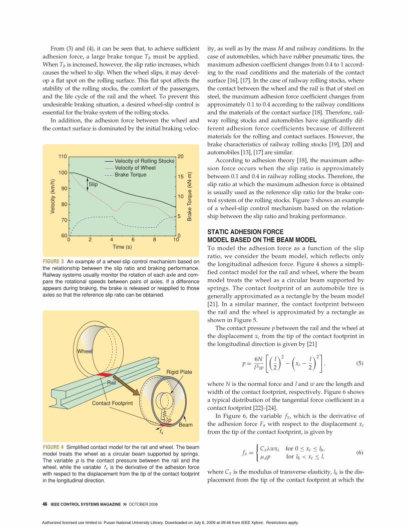
According to adhesion theory [18], the maximum adhe-sion force occurs when the slip ratio is approximatelybetween 0.1 and 0.4 in railway rolling stocks. Therefore, theslip ratio at which the maximum adhesion force is obtainedis usually used as the reference slip ratio for the brake con-trol system of the rolling stocks. Figure 3 shows an exampleof a wheel-slip control mechanism based on the relation-ship between the slip ratio and braking performance.

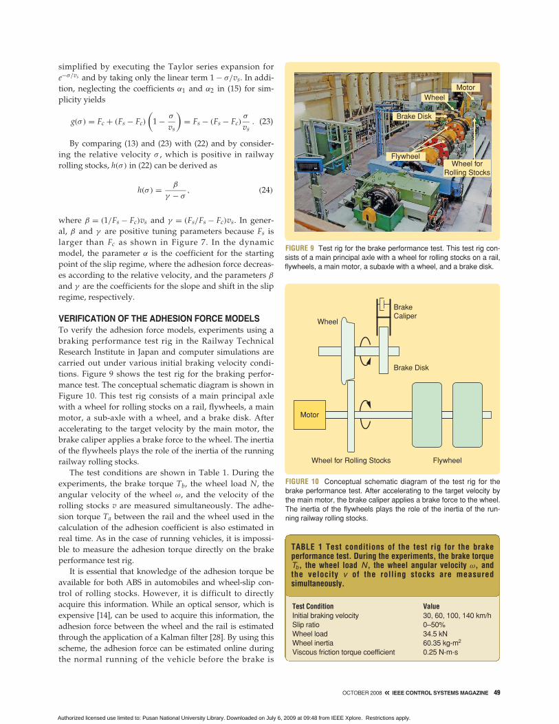
STATIC ADHESION FORCEMODEL BASED ON THE BEAM MODELTo model the adhesion force as a function of the slipratio, we consider the beam model, which reflects onlythe longitudinal adhesion force. Figure 4 shows a simpli-fied contact model for the rail and wheel, where the beammodel treats the wheel as a circular beam supported bysprings. The contact footprint of an automobile tire isgenerally approximated as a rectangle by the beam model[21]. In a similar manner, the contact footprint betweenthe rail and the wheel is approximated by a rectangle asshown in Figure 5.

The contact pressure p between the rail and the wheel atthe displacement xc from the tip of the contact footprint inthe longitudinal direction is given by [21]

p = 6Nl3w

[(l2

)2−

(xc − l

2

)2]

, (5)

where N is the normal force and l and w are the length andwidth of the contact footprint, respectively. Figure 6 showsa typical distribution of the tangential force coefficient in acontact footprint [22]–[24].

In Figure 6, the variable fx, which is the derivative ofthe adhesion force Fa with respect to the displacement xc

from the tip of the contact footprint, is given by

fx ={

Cxλwxc for 0 ≤ xc ≤ lh,μdp for lh < xc ≤ l,

(6)

where Cx is the modulus of transverse elasticity, lh is the dis-placement from the tip of the contact footprint at which the

FIGURE 3 An example of a wheel-slip control mechanism based onthe relationship between the slip ratio and braking performance.Railway systems usually monitor the rotation of each axle and com-pare the rotational speeds between pairs of axles. If a differenceappears during braking, the brake is released or reapplied to thoseaxles so that the reference slip ratio can be obtained.

Slip

110

100

90

80

70

600 2 4

Time (s)

Bra

ke T

orqu

e (k

N-m

)

Vel

ocity

(km

/h)

6 8 10

20

15

10

5

0

Velocity of Rolling StocksVelocity of WheelBrake Torque

FIGURE 4 Simplified contact model for the rail and wheel. The beammodel treats the wheel as a circular beam supported by springs.The variable p is the contact pressure between the rail and thewheel, while the variable fx is the derivative of the adhesion forcewith respect to the displacement from the tip of the contact footprintin the longitudinal direction.

Wheel

Rail

Beamp

Rigid Plate

Contact Footprint

fx

46 IEEE CONTROL SYSTEMS MAGAZINE » OCTOBER 2008


adhesion-force derivative fx changes rapidly, and μd is thedynamic friction coefficient. In particular, μd is defined by

μd = μmax − aλvl(l − lh)

, (7)

where μmax is the maximum adhesion coefficient, a is aconstant that determines the dynamic friction coefficient inthe slipping regime, and lh is expressed as [21]

lh = l(

1 − Kxλ

3μmaxN

), (8)

where Kx is the traveling stiffness calculated by

Kx = 12

Cxl2. (9)

The wheel load, which is the normal force, is equal tothe integrated value of the contact pressure between therail and the wheel over the contact footprint. Therefore, theadhesion force Fa between the rail and the wheel can becalculated by integrating (6) over the length of the contactfootprint and substituting (7) and (8) into (6), which isexpressed as

Fa = 12

Cxλwl2(

1 − Kxλ

3μmaxN

)2

+ 12

Kxλ − 32

Na(v − rω)

− 12μmaxN

[1 − 3

Na(v − rω)

Kxλ

][1 −

(1 − 2Kxλ

3μmaxN

)3].

(10)

DYNAMIC ADHESION FORCEMODEL BASED ON BRISTLE CONTACTAs a dynamic adhesion force model, we consider the Dahlmodel given by [25]

dzdt

= σ − α |σ |Fc

z , (11)

F = αz , (12)

where z is the internal friction state, σ is the relative velocity,α is the stiffness coefficient, and F and Fc are the friction forceand Coulomb friction force, respectively. Since the steady-state version of the Dahl model is equivalent to Coulomb fric-tion, the Dahl model is a generalized model for Coulombfriction. However, the Dahl model does not capture either theStribeck effect or stick-slip effects. In fact, the friction behaviorof the adhesion force according to the relative velocity σ forrailway rolling stocks exhibits the Stribeck effect, as shown inFigure 7. Therefore, the Dahl model is not suitable as anadhesion force model for railway rolling stocks.

However, the LuGre model [11], which is a generalizedform of the Dahl model, can describe both the Stribeckeffect and stick-slip effects. The LuGre model equations aregiven by

dzdt

= σ − α|σ |g(σ )

z , (13)

g(σ ) = Fc + (Fs − Fc)e−(σ/vs)2, (14)

F = αz + α1 z + α2σ , (15)


FIGURE 5 Contact footprint between the rail and the wheel. Theshape of this footprint can be approximated by a rectangle. Thelength and width of the contact footprint are both approximately1.9 cm. This value is used to calculate the contact pressurebetween the rail and the wheel as well as the adhesion force.

1.9 cm

FIGURE 6 A typical distribution of the tangential force coefficient in acontact footprint. In the locking regime, the adhesion-force derivativefx increases linearly according to the displacement of the contactfootprint. However, in the slipping regime, the adhesion-force deriva-tive fx is proportional to the contact pressure. The adhesion force Fa

can be calculated by integrating the adhesion-force derivative fx

over the length of the contact footprint.

Slipping RegimeLocking Regime

lh l0

Displacement of the Contact Footprint xc

Adh

esio

n-F

orce

Der

ivat

ive

f x

fx = Cx wxcλ

fx = dpμ


where z is the average bristle deflection, vs is the Stribeckvelocity, and Fs is the static friction force. In addition, α, α1,and α2 are the bristle stiffness coefficient, bristle dampingcoefficient, and viscous damping coefficient, respectively.

The functions g(σ ) and F in (14) and (15) are deter-mined by selecting the exponential term in (14) and coeffi-cients α , α1 , and α2 in (15), respectively, to match themathematical model with the measured friction. For exam-ple, to match the mathematical model with the measuredfriction, the standard LuGre model is modified by usinge−|σ/vs|1/2

in place of the term e−(σ/vs)2in (14). Furthermore,

for the tire model for vehicle traction control, the functionF given by (15) is modified by including the normal force.Thus, (13)–(15) are modified as [26]

dzdt

= σ − α′|σ |g(σ )

z , (16)

g(σ ) = μc + (μs − μc)e−|σ/vs|12

, (17)

F = (α′z + α′1 z + α′

2σ)N , (18)

where μs and μc are the static friction coefficient andCoulomb friction coefficient, respectively, N = mg is thenormal force, m is the mass of the wheel, and α′ = α/N,α′

1 = α1/N, and α′2 = α2/N are the normalized wheel longi-

tudinal lumped stiffness coefficient, normalized wheel lon-gitudinal lumped damping coefficient, and normalizedviscous damping coefficient, respectively.

In general, it is difficult to measure and identify all sixparameters, α, α1, α2, Fs, Fc, and vs in the LuGre modelequations. In particular, identifying friction coefficientssuch as α and α1 requires a substantial amount of experi-mental data [27]. We thus develop a dynamic model forfriction phenomena in railway rolling stocks, as shown inFigure 7. The dynamic model retains the simplicity of theDahl model while capturing the Stribeck effect.

As shown in Figure 8 [11], the motion of the bristles isassumed to be the stress-strain behavior in solid mechan-ics, which is expressed as

dFa

dx= α [1 − h(σ )Fa] , (19)

where Fa is the adhesion force, α is the coefficient of thedynamic adhesion force, and x and σ are the relative dis-placement and velocity of the contact surface, respectively.In addition, the function h(σ ) is selected according to thefriction characteristics.

Defining z to be the average deflection of the bristles,the adhesion force Fa is assumed to be given by

Fa = αz. (20)

The derivative of Fa can then be expressed as

dFa

dt= dFa

dxdxdt

= dFa

dxσ = α[1 − h(σ )Fa]σ = α

dzdt

. (21)

It follows from (20) and (21) that the internal state z isgiven by

z = σ [1 − h(σ )Fa] = σ [1 − αh(σ )z]. (22)

To select the function h(σ ) for railway rolling stocks, theterm e−σ/vs is used in place of e−(σ/vs)

2in (14). This term is

FIGURE 8 Bristle model between the rail and the wheel. The frictioninterface between the rail and the wheel is modeled as contactbetween bristles. For simplicity the bristles on the lower part areshown as being rigid. [11].

Rail

z

νWheel

Wheel

Rail

FIGURE 7 Typical shape of the general friction force and adhesionforce in railway rolling stocks according to the relative velocity. Stat-ic friction, Coulomb friction, the Stribeck effect, and viscous frictionare included in the general friction force, while static friction,Coulomb friction, and the Stribeck effect are included in the adhe-sion force in railway rolling stocks.

Stribeck Effect

For

ce F

0

Fc

Fs

General Friction Force

Railway AdhesionForce

Relative Velocity σ


Two kinds of models, namely, the beam and bristle models,

for the adhesion force in railway rolling stocks are developed.


simplified by executing the Taylor series expansion fore−σ/vs and by taking only the linear term 1 − σ/vs. In addi-tion, neglecting the coefficients α1 and α2 in (15) for sim-plicity yields

g(σ ) = Fc + (Fs − Fc)

(1 − σ

vs

)= Fs − (Fs − Fc)

σ

vs. (23)

By comparing (13) and (23) with (22) and by consider-ing the relative velocity σ , which is positive in railwayrolling stocks, h(σ ) in (22) can be derived as

h(σ ) = β

γ − σ, (24)

where β = (1/Fs − Fc)vs and γ = (Fs/Fs − Fc)vs. In gener-al, β and γ are positive tuning parameters because Fs islarger than Fc as shown in Figure 7. In the dynamicmodel, the parameter α is the coefficient for the startingpoint of the slip regime, where the adhesion force decreas-es according to the relative velocity, and the parameters βand γ are the coefficients for the slope and shift in the slipregime, respectively.

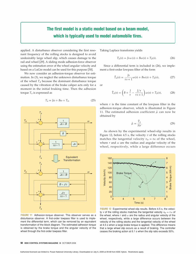
VERIFICATION OF THE ADHESION FORCE MODELSTo verify the adhesion force models, experiments using abraking performance test rig in the Railway TechnicalResearch Institute in Japan and computer simulations arecarried out under various initial braking velocity condi-tions. Figure 9 shows the test rig for the braking perfor-mance test. The conceptual schematic diagram is shown inFigure 10. This test rig consists of a main principal axlewith a wheel for rolling stocks on a rail, flywheels, a mainmotor, a sub-axle with a wheel, and a brake disk. Afteraccelerating to the target velocity by the main motor, thebrake caliper applies a brake force to the wheel. The inertiaof the flywheels plays the role of the inertia of the runningrailway rolling stocks.

The test conditions are shown in Table 1. During theexperiments, the brake torque Tb, the wheel load N, theangular velocity of the wheel ω, and the velocity of therolling stocks v are measured simultaneously. The adhe-sion torque Ta between the rail and the wheel used in thecalculation of the adhesion coefficient is also estimated inreal time. As in the case of running vehicles, it is impossi-ble to measure the adhesion torque directly on the brakeperformance test rig.

It is essential that knowledge of the adhesion torque beavailable for both ABS in automobiles and wheel-slip con-trol of rolling stocks. However, it is difficult to directlyacquire this information. While an optical sensor, which isexpensive [14], can be used to acquire this information, theadhesion force between the wheel and the rail is estimatedthrough the application of a Kalman filter [28]. By using thisscheme, the adhesion force can be estimated online duringthe normal running of the vehicle before the brake is


FIGURE 9 Test rig for the brake performance test. This test rig con-sists of a main principal axle with a wheel for rolling stocks on a rail,flywheels, a main motor, a subaxle with a wheel, and a brake disk.

WheelMotor

Brake Disk

FlywheelWheel for

Rolling Stocks

FIGURE 10 Conceptual schematic diagram of the test rig for thebrake performance test. After accelerating to the target velocity bythe main motor, the brake caliper applies a brake force to the wheel.The inertia of the flywheels plays the role of the inertia of the run-ning railway rolling stocks.

Flywheel

Motor

Wheel for Rolling Stocks

Wheel

Brake Disk

BrakeCaliper

TABLE 1 Test conditions of the test rig for the brakeperformance test. During the experiments, the brake torqueTb, the wheel load N, the wheel angular velocity ω, andthe velocity v of the rolling stocks are measuredsimultaneously.

Test Condition ValueInitial braking velocity 30, 60, 100, 140 km/hSlip ratio 0–50%Wheel load 34.5 kNWheel inertia 60.35 kg-m2

Viscous friction torque coefficient 0.25 N-m-s


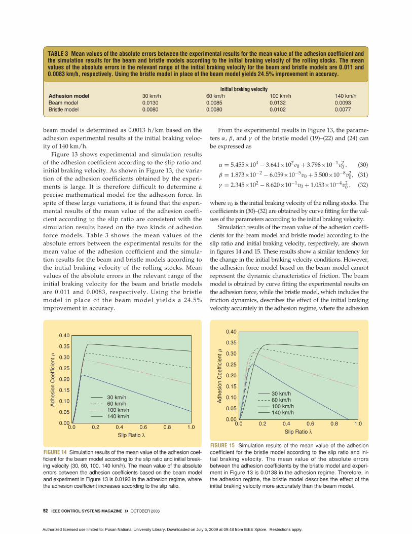
applied. A disturbance observer considering the first reso-nant frequency of the rolling stocks is designed to avoidundesirably large wheel slip, which causes damage to therail and wheel [29]. A sliding mode adhesion-force observerusing the estimation error of the wheel angular velocity andbased on a LuGre model can be used for this purpose [30].

We now consider an adhesion-torque observer for esti-mation. In (3), we neglect the unknown disturbance torqueof the wheel Td because the dominant disturbance torquecaused by the vibration of the brake caliper acts only for amoment in the initial braking time. Then the adhesiontorque Ta is expressed as

Ta = Jω + Bω + Tb. (25)

Taking Laplace transforms yields

Ta(s) = Jsω (s) + Bω(s) + Tb(s). (26)

Since a differential term is included in (26), we imple-ment a first-order lowpass filter of the form

Ta(s) = Jsτ s + 1

ω(s) + Bω(s) + Tb(s), (27)

or

Ta(s) =(

B + Jτ

− J/τ

τ s + 1

)ω(s) + Tb(s), (28)

where τ is the time constant of the lowpass filter in theadhesion-torque observer, which is illustrated in Figure11. The estimated adhesion coefficient μ can now beobtained by

μ = Ta

Nr. (29)

As shown by the experimental wheel-slip results inFigure 12, before 4.5 s, the velocity v of the rolling stocksmatches the tangential velocity vw = rω of the wheel,where r and ω are the radius and angular velocity of thewheel, respectively, while a large difference occurs

FIGURE 11 Adhesion-torque observer. This observer serves as adisturbance observer. A first-order lowpass filter is used to imple-ment the differential term, which can be removed by an equivalenttransformation of the block diagram. The estimated adhesion torqueis obtained by the brake torque and the angular velocity of thewheel through the first-order lowpass filter.

FIGURE 12 Experimental wheel-slip results. Before 4.5 s, the veloci-ty v of the rolling stocks matches the tangential velocity vw = r ω ofthe wheel, where r and ω are the radius and angular velocity of thewheel, respectively, while a large difference occurs between thevelocity of the rolling stocks and the tangential velocity of the wheelat 4.5 s when a large brake torque is applied. This difference meansthat a large wheel slip occurs as a result of braking. The controllerceases the braking action at 6.1 s when the slip ratio exceeds 50%.

160

140

120

100

80

Vel

ocity

(km

/h)

60

40

20

03 4 5

Time (s)

6 7 8

8

7

6

5

4

Bra

ke T

orqu

e (k

N-m

)

3

2

1

0

Brake Torque

w

ν

ν


Js

Ta

Tb

Tb

ω

Ta

Taˆ

Taˆ

EquivalentTransformation

1Js + B

B

++

+−

+

ω

−+

+−

+

1Js + B

B + J/τ

s + 1J/τ

τ

1s + 1τ

The first model is a static model based on a beam model,

which is typically used to model automobile tires.


between the velocity of the rolling stocks and the tangen-tial velocity of the wheel at 4.5 s when a large brake torqueis applied. This difference means that large wheel slipoccurs as a result of braking. The controller ceases thebraking action at 6.1 s when the slip ratio exceeds 50%.Henceforth, the tangential velocity of the wheel recovers,and the slip ratio decreases to zero by the adhesion forcebetween the rail and the wheel. In the experiment, to pre-vent damage due to excessive wheel slip, the applied braketorque is limited so that the slip ratio does not exceed 50%.

Table 2 shows the parameters of the adhesion forcemodels for computer simulation. In Table 2, the parame-ter values for the length l and the width w of the contactfootprint are taken from [31]. The constant a in (7) for the


TABLE 2 Parameters of the beam and bristle models forcomputer simulation. The parameter values for the length land width w of the contact footprint are taken from [31].The velocity v0 is the initial braking velocity of the rollingstocks.

Parameter Notation ValueModulus of transverse elasticity Cx 1.52 × 109 N/m2

Length l 0.019 mWidth w 0.019 mWheel load N 34.5 kNMaximum adhesion coefficient μmax 0.360, 0.310,

for v0 = 30, 60, 100, 140 km/h 0.261, 0.226Radius of the wheel r 0.43 m

FIGURE 13 Experimental and simulation results of the adhesion coefficient according to the slip ratio and initial braking velocity. The sym-bols “�”, “◦”, and “×” represent the maximum, mean, and minimum values of the adhesion coefficient, respectively, which are obtainedby experiments. Compared with the experimental results, the bristle model describes the adhesion coefficient more accurately accordingto the slip ratio and initial braking than the beam model. (a) Initial braking velocity v0 = 140 km/h. (b) Initial braking velocity v0 = 100 km/h.(c) Initial braking velocity v0 = 60 km/h. (d) Initial braking velocity v0 = 30 km/h.

Experimental ResultsBristle ModelBeam Model

1.00.80.60.4

Slip Ratio λ

(d)

0.20.00.00

0.05

0.10

0.15

0.20

0.25

0.30

0.35

0.40

Adh

esio

n C

oeffi

cien

t μ


1.00.80.60.4

Slip Ratio λ

(c)

0.20.00.00

0.05

0.10

0.15

0.20

0.25

0.30

0.35

0.40

Adh

esio

n C

oeffi

cien

t μ


1.00.80.60.4Slip Ratio λ

(b)

0.20.00.00

0.05

0.10

0.15

0.20

0.25

0.30

0.35

0.40

Adh

esio

n C

oeffi

cien

t μ



(a)

0.20.00.00

0.05

0.10

0.15

0.20

0.25

0.30

0.35

0.40

Adh

esio

n C

oeffi

cien

t μ


beam model is determined as 0.0013 h/km based on theadhesion experimental results at the initial braking veloc-ity of 140 km/h.

Figure 13 shows experimental and simulation resultsof the adhesion coefficient according to the slip ratio andinitial braking velocity. As shown in Figure 13, the varia-tion of the adhesion coefficients obtained by the experi-ments is large. It is therefore difficult to determine aprecise mathematical model for the adhesion force. Inspite of these large variations, it is found that the experi-mental results of the mean value of the adhesion coeffi-cient according to the slip ratio are consistent with thesimulation results based on the two kinds of adhesionforce models. Table 3 shows the mean values of theabsolute errors between the experimental results for themean value of the adhesion coefficient and the simula-tion results for the beam and bristle models according tothe initial braking velocity of the rolling stocks. Meanvalues of the absolute errors in the relevant range of theinitial braking velocity for the beam and bristle modelsare 0.011 and 0.0083, respectively. Using the bristlemodel in place of the beam model yields a 24.5%improvement in accuracy.

From the experimental results in Figure 13, the parame-ters α, β , and γ of the bristle model (19)–(22) and (24) canbe expressed as

α = 5.455×104 − 3.641×102v0 + 3.798×10−1v20 , (30)

β = 1.873×10−2 − 6.059×10−5v0 + 5.500×10−8v20, (31)

γ = 2.345×102 − 8.620×10−1v0 + 1.053×10−4v20 , (32)

where v0 is the initial braking velocity of the rolling stocks. Thecoefficients in (30)–(32) are obtained by curve fitting for the val-ues of the parameters according to the initial braking velocity.

Simulation results of the mean value of the adhesion coeffi-cients for the beam model and bristle model according to theslip ratio and initial braking velocity, respectively, are shownin figures 14 and 15. These results show a similar tendency forthe change in the initial braking velocity conditions. However,the adhesion force model based on the beam model cannotrepresent the dynamic characteristics of friction. The beammodel is obtained by curve fitting the experimental results onthe adhesion force, while the bristle model, which includes thefriction dynamics, describes the effect of the initial brakingvelocity accurately in the adhesion regime, where the adhesion

FIGURE 14 Simulation results of the mean value of the adhesion coef-ficient for the beam model according to the slip ratio and initial break-ing velocity (30, 60, 100, 140 km/h). The mean value of the absoluteerrors between the adhesion coefficients based on the beam modeland experiment in Figure 13 is 0.0193 in the adhesion regime, wherethe adhesion coefficient increases according to the slip ratio.

30 km/h

100 km/h60 km/h

140 km/h

1.00.80.60.4

Slip Ratio λ0.20.0

0.00

0.05

0.10

0.15

0.20

0.25

0.30

0.35

0.40

Adh

esio

n C

oeffi

cien

t μ

TABLE 3 Mean values of the absolute errors between the experimental results for the mean value of the adhesion coefficient andthe simulation results for the beam and bristle models according to the initial braking velocity of the rolling stocks. The meanvalues of the absolute errors in the relevant range of the initial braking velocity for the beam and bristle models are 0.011 and0.0083 km/h, respectively. Using the bristle model in place of the beam model yields 24.5% improvement in accuracy.

Initial braking velocityAdhesion model 30 km/h 60 km/h 100 km/h 140 km/hBeam model 0.0130 0.0085 0.0132 0.0093Bristle model 0.0080 0.0080 0.0102 0.0077

FIGURE 15 Simulation results of the mean value of the adhesioncoefficient for the bristle model according to the slip ratio and ini-tial braking velocity. The mean value of the absolute errorsbetween the adhesion coefficients by the bristle model and experi-ment in Figure 13 is 0.0138 in the adhesion regime. Therefore, inthe adhesion regime, the bristle model describes the effect of theinitial braking velocity more accurately than the beam model.

30 km/h

100 km/h60 km/h

140 km/h

1.00.80.60.4

Slip Ratio λ0.20.0

0.00

0.05

0.10

0.15

0.20

0.25

0.30

0.35

0.40

Adh

esio

n C

oeffi

cien

t μ



force increases according to the slip ratio, as shown in Figure15. Therefore, the bristle model is more applicable than thebeam model for the desired wheel-slip controller design.

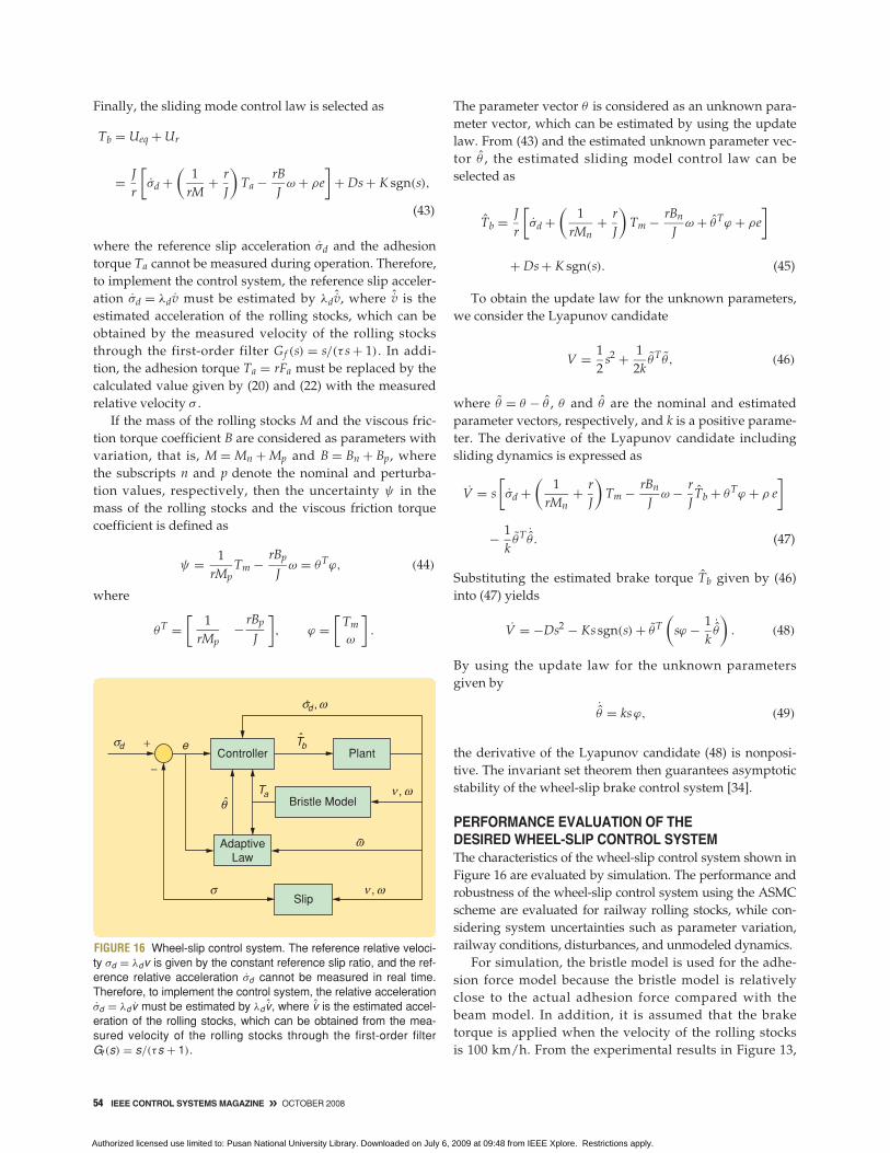
DESIRED WHEEL SLIP USINGADAPTIVE SLIDING MODE CONTROL The desired wheel-slip brake control system is designed byusing an ASMC scheme to achieve robust wheel-slip brakecontrol. In the controller design process, the random valueof adhesion torque, the disturbance torque due to the vibra-tion of the brake caliper, and the traveling resistance forceof the rolling stocks are considered as system uncertainties.The mass of the rolling stocks and the viscous frictiontorque coefficient are also considered as parameters withunknown variations. The adaptive law for the unknownparameters is based on Lyapunov stability theory.

The sliding surface s for the design of the adaptive slid-ing mode wheel-slip brake control system is defined as

s = e + ρ

∫ t

0e dt, (33)

where e = σd − σ is the tracking error of the relative veloci-ty, σ = λv = v − rω is the relative velocity, σd is the refer-ence relative velocity, and ρ is a positive design parameter.

The sliding mode control law consists of equivalent androbust control terms, that is,

Tb = Ueq + Ur, (34)

where Ueq and Ur are the equivalent and robust controlterms. To obtain Ueq and Ur, we combine (3), (4) with thederivative of the sliding surface in (33) and include randomterms in the adhesion force Far = Fa + Fr and the adhesiontorque Tar = Ta + Tr, where Fr and Tr are the random termsof the adhesion force and adhesion torque, respectively.Then, the derivative of the sliding surface can be written as

s = σd +(

1rM

+ rJ

)Ta +

(1

rM+ r

J

)Tr + 1

MFr

− rJTb − rB

Jω − r

JTd + ρ e . (35)

To determine the equivalent control term Ueq, uncer-tainties such as random terms in the adhesion force andadhesion torque Fr and Tr , as well as the disturbancetorque Td in (35) are neglected, and it is assumed that the

sliding surface s is at steady state, that is, s = 0, then theequivalent control law can be determined as

Ueq = Jr

[σd +

(1

rM+ r

J

)Ta − rB

Jω + ρe

]. (36)

Thus, s can be rewritten as

s =(

1rM

+ rJ

)Tr + 1

MFr − r

JTd − r

JUr. (37)

In the standard sliding mode control, to satisfy thereachability condition that directs system trajectoriestoward a sliding surface where they remain, the derivativeof the sliding surface is selected as

s = −K sgn(s). (38)

In this case, chattering occurs in the control input. Toattenuate chattering in the control input, the derivative ofthe sliding surface is selected as [32], [33]

s = −Ds − K sgn(s), (39)

where the parameters D and K are positive.To determine a control term Ur that achieves robustness

to uncertainties such as random terms in the adhesionforce and adhesion torque, as well as the disturbancetorque, it is assumed that

D0 |s| + K0 >

∣∣∣∣(

1rM

+ rJ

)Tr + 1

MFr − r

JTd

∣∣∣∣ + η, (40)

where the parameters D0 = (r/J)D, K0 = (r/J)K, and η arepositive. Then, the robust control law can be determined as

Ur = Ds + K sgn( s), (41)

and using (40), the reachability condition is satisfied as

ss = s[(

1rM

+ rJ

)Tr + 1

MFr − r

JTd − D0s − K0 sgn(s)

]

≤ |s|[∣∣∣∣

(1

rM+ r

J

)Tr + 1

MFr − r

JTd

∣∣∣∣ − D0 |s| − K0

]

< −η|s|. (42)


The second model is a dynamic model based on a bristle model,

in which the friction interface between the rail and the wheel is

modeled as contact between bristles.


Finally, the sliding mode control law is selected as

Tb = Ueq + Ur

= Jr

[σd +

(1

rM+ r

J

)Ta − rB

Jω + ρe

]+ Ds + K sgn(s),

(43)

where the reference slip acceleration σd and the adhesiontorque Ta cannot be measured during operation. Therefore,to implement the control system, the reference slip acceler-ation σd = λdv must be estimated by λd ˆv, where ˆv is theestimated acceleration of the rolling stocks, which can beobtained by the measured velocity of the rolling stocksthrough the first-order filter Gf (s) = s/(τ s + 1). In addi-tion, the adhesion torque Ta = rFa must be replaced by thecalculated value given by (20) and (22) with the measuredrelative velocity σ .

If the mass of the rolling stocks M and the viscous fric-tion torque coefficient B are considered as parameters withvariation, that is, M = Mn + Mp and B = Bn + Bp, wherethe subscripts n and p denote the nominal and perturba-tion values, respectively, then the uncertainty ψ in themass of the rolling stocks and the viscous friction torquecoefficient is defined as

ψ = 1rMp

Tm − rBp

Jω = θTϕ, (44)

where

θT =[

1rMp

− rBp

J

], ϕ =

[Tm

ω

].

The parameter vector θ is considered as an unknown para-meter vector, which can be estimated by using the updatelaw. From (43) and the estimated unknown parameter vec-tor θ , the estimated sliding model control law can beselected as

Tb = Jr

[σd +

(1

rMn+ r

J

)Tm − rBn

Jω + θTϕ + ρe

]

+ Ds + K sgn(s). (45)

To obtain the update law for the unknown parameters,we consider the Lyapunov candidate

V = 12

s2 + 12k

θTθ , (46)

where θ = θ − θ , θ and θ are the nominal and estimatedparameter vectors, respectively, and k is a positive parame-ter. The derivative of the Lyapunov candidate includingsliding dynamics is expressed as

V = s[σd +

(1

rMn+ r

J

)Tm − rBn

Jω − r

JTb + θTϕ + ρ e

]

− 1kθT ˙

θ. (47)

Substituting the estimated brake torque Tb given by (46)into (47) yields

V = −Ds2 − Kssgn(s) + θT(

sϕ − 1k

˙θ

). (48)

By using the update law for the unknown parametersgiven by

˙θ = ksϕ, (49)

the derivative of the Lyapunov candidate (48) is nonposi-tive. The invariant set theorem then guarantees asymptoticstability of the wheel-slip brake control system [34].

PERFORMANCE EVALUATION OF THEDESIRED WHEEL-SLIP CONTROL SYSTEMThe characteristics of the wheel-slip control system shown inFigure 16 are evaluated by simulation. The performance androbustness of the wheel-slip control system using the ASMCscheme are evaluated for railway rolling stocks, while con-sidering system uncertainties such as parameter variation,railway conditions, disturbances, and unmodeled dynamics.

For simulation, the bristle model is used for the adhe-sion force model because the bristle model is relativelyclose to the actual adhesion force compared with thebeam model. In addition, it is assumed that the braketorque is applied when the velocity of the rolling stocksis 100 km/h. From the experimental results in Figure 13,

FIGURE 16 Wheel-slip control system. The reference relative veloci-ty σd = λdv is given by the constant reference slip ratio, and the ref-erence relative acceleration σd cannot be measured in real time.Therefore, to implement the control system, the relative accelerationσd = λdv must be estimated by λd ˆv, where ˆv is the estimated accel-eration of the rolling stocks, which can be obtained from the mea-sured velocity of the rolling stocks through the first-order filterGf (s) = s/(τs + 1).

Slip,

,ν ω

ν ω

,ω

σ

ω

σ

θ

bT

aTBristle Model

Plante

Controller

AdaptiveLaw

−

+d

σd.



it is assumed that the random adhesion force Fr is awhite noise signal with a Gaussian distribution that hasa standard deviation of 0.431 kN. Since the actual brakeforce is applied to the wheel disk by the brake caliper,the vibration occurs on the brake caliper at the initialbraking moment. Therefore, the disturbance torqueTd = 0.05Tbe−4t sin 10πt, caused by the vibration of thebrake caliper, is considered in the simulation. In addi-tion, the traveling resistance force Fr = 0.63v2 of therolling stocks and the viscous friction B = 0.25−0.01t isconsidered, which causes overheating between the wheeldisk and the brake pad. Finally, the unmodeled dynam-ics Ga (s) = e−0.15s/(0.6s + 1) of the pneumatic actuator ofthe brake control system are considered.

To assess the braking performance in the presence ofparameter variations, the simulation is carried out underthe assumption that the mass of the rolling stocks changesaccording to the number of passengers and that the rollingstocks travel in dry or wet rail conditions. It is assumedthat the mass of the rolling stocks changes from 3517 to5276 kg at 25 s. It is also assumed that the maximum adhe-sion force under wet rail conditions is approximately halfof the maximum adhesion force under dry rail conditionsand that the rail conditions change from dry to wet at 25 s.Figure 17 shows the relationship between the adhesionforce coefficient and the slip ratio according to the changein rail conditions from dry to wet based on the beam andbristle models, which are considered in the simulation. Asshown in Figure 17, the reference slip ratio is assumed tobe 0.119 and 0.059 under dry and wet rail conditions,respectively, for the beam model, and 0.132 and 0.092under dry and wet rail conditions, respectively, for thebristle model.

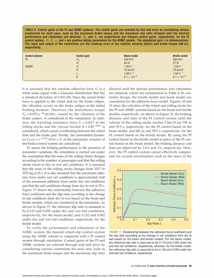
To verify the performance and robustness of theASMC system, the desired wheel-slip control systemusing the ASMC scheme is compared with a PI controlsystem through simulation. Control gains of the PI andASMC systems are selected through trial and error byconsidering various constraints for each case, such asthe maximum brake torque and the maximum slip ratio

allowed until the desired performance and robustnessare obtained, which are summarized in Table 4. In con-troller design, the bristle model and beam model areconsidered for the adhesion force model. Figures 18 and19 show the velocities of the wheel and rolling stocks forthe PI and ASMC systems based on the beam and bristlemodels, respectively. As shown in Figure 18, the brakingdistance and time of the PI control system until thevelocity of the rolling stocks reaches 5 km/h are 700 mand 59.5 s, respectively, for the PI control based on thebeam model, and 682 m and 58.9 s, respectively, for thePI control based on the bristle model. By using the PIcontrol based on the bristle model in place of the PI con-trol based on the beam model, the braking distance andtime are improved by 2.6% and 1%, respectively. How-ever, the PI control system cannot effectively compen-sate for system uncertainties such as the mass of the

FIGURE 17 Relationship between the adhesion force coefficient andthe slip ratio according to the change in rail conditions from dry towet based on the beam and bristle models. For the beam model,the reference slip ratio is assumed to be 0.119 and 0.059 under dryand wet rail conditions, respectively, whereas, for the bristle model,the reference slip ratio is assumed to be 0.132 and 0.092 under dryand wet rail conditions, respectively.

Bristle Model (Dry)Bristle Model (Wet)Beam Model (Dry)Beam Model (Wet)


0.10.00.0

0.1

0.2

0.3

0.4

0.5

Adh

esio

n F

orce

Coe

ffici

ent

μ


TABLE 4 Control gains of the PI and ASMC systems. The control gains are selected by trial and error by considering variousconstraints for each case, such as the maximum brake torque and the maximum slip ratio allowed until the desiredperformance and robustness are obtained. Kp and Ki are proportional and integral control gains, respectively, for the PIcontrol system. D, K , ρ, and k are positive design parameters for the ASMC system. The adaptation gain k is dimensionless.The input and output of the controllers are the tracking error of the relative velocity (km/h) and brake torque (kN-m),respectively.

Control scheme Control gain Beam model Bristle modelPI Kp 400 N-h 650 N-h

Ki 54 N 27 NASMC D 1.62 h−1 1.53 h−1

K 70 km/h2 70 km/h2

ρ 1.65 h−1 1.54 h−1

k 2.1 × 10−8 2.1 × 10−8


rolling stocks, railway conditions, the traveling resistanceforce, and variations of the viscous friction coefficient.

As shown in Figure 19 for the ASMC system, the brak-ing distance and time are 607 m and 55.3 s, respectively,for the ASMC based on the beam model and 581 m and50.7 s, respectively, for the ASMC based on the bristlemodel. Figure 19 shows that the ASMC system providesrobust velocity regulation of the rolling stocks in the pres-ence of variations in the mass of the rolling stocks and railconditions. In this case, the braking distance and time areimproved by 4.3% and 8.3%, respectively, by using theASMC based on the bristle model in place of the ASMCbased on the beam model.

Figure 20 shows the brake torques for the PI and ASMCsystems based on the beam and bristle models. Theexpended braking energies of the PI and ASMC systemsduring braking time are 1.77 × 107 N-m and 1.71 × 107 N-m, respectively. Therefore, by using the ASMC system, it ispossible to effectively reduce the braking time and dis-tance using a relatively small braking energy consumption.

The operation of the PI and ASMC wheel-slip controlsystems can also be demonstrated through the slip ratios.Figure 21 shows the slip ratios of the PI and ASMC sys-

tems based on the beam and bristle models. Figure 21shows that the PI control system has a large tracking errorof slip ratio compared with the ASMC system. However,the wheel-slip control system using the ASMC scheme canmaintain the slip ratio near the reference slip ratio duringthe braking time although the slip ratios fluctuate slightlyafter 25 s when the system uncertainties are applied.Therefore, it is appropriate to use the ASMC system toobtain the maximum adhesion force and a short brakingdistance. Using the ASMC based on the bristle model inplace of the PI control based on the beam model yields28% improvement in the wheel slip. Table 5 summarizesthe performance of the PI and ASMC systems based on thebeam and bristle models.

CONCLUSIONSTwo types of models, namely, the beam and bristlemodels, for the adhesion force in railway rolling stocksare developed. The validity of the beam and bristlemodels is determined through an adhesion test using abrake performance test rig. By comparing the simulationresults of the two types of adhesion force models withthe experimental results, it is found that these adhesion


FIGURE 18 Velocities of the wheel and rolling stocks for the propor-tional-integral (PI) control systems based on the beam and bristlemodels. For the PI control based on the beam model, the brakingdistance and time of the PI control system until the velocity of therolling stocks reaches 5 km/h are 700 m and 59.5 s, respectively,and 682 m and 58.9 s, respectively, for the PI control based on thebristle model. By using the PI control based on the bristle model inplace of the PI control based on the beam model, the braking dis-tance and time are improved by 2.6% and 1%, respectively.

Rolling Stocks (Bristle Model)Wheel (Bristle Model)Rolling Stocks (Beam Model)Wheel (Beam Model)

50403020

Time (s)

1000

40

30

20

10

50

60

70

80

90

100

110

Vel

ocity

(km

/h)

FIGURE 19 Velocities of the wheel and rolling stocks for the adaptivesliding mode control (ASMC) systems based on the beam and bris-tle models. For the ASMC based on the beam model, the brakingdistance and time of the ASMC system until the velocity of therolling stocks reaches 5 km/h are 607 m and 55.3 s, respectively,and 581 m and 50.7 s, respectively, for the ASMC based on thebristle model. By using the ASMC based on the bristle model inplace of the ASMC based on the beam model, the braking distanceand time are improved by 4.3% and 8.3%, respectively.

Rolling Stocks (Bristle Model)Wheel (Bristle Model)Rolling Stocks (Beam Model)Wheel (Beam Model)

50403020

Time (s)

1000

40

30

20

10

50

60

70

80

90

100

110

Vel

ocity

(km

/h)

The validity of the beam and bristle models is determined through

an adhesion test using a brake performance test rig.



force models can effectively represent the experimentalresults. However, the adhesion force model based on thebeam model cannot represent the dynamic characteris-tics of friction, while the bristle model can mathemati-cally include the dynamics on friction and can preciselyconsider the effect of the initial braking velocity in theadhesion regime. Therefore, the bristle model is moreappropriate than the beam model for the design of thewheel-slip controller.

In addition, based on the beam and bristle models,the PI and ASMC systems are designed to control wheelslip in railway rolling stocks. Through simulation, we

evaluate the performance and robustness of the PI andASMC systems based on the beam and bristle modelsfor railway rolling stocks. It is verified from the simula-tion study that, among the four types investigatedaccording to control schemes and adhesion force mod-els, the ASMC system based on the bristle model is themost suitable system for the wheel slip in the rollingstocks with system uncertainties such as the mass andtraveling resistance force of the rolling stocks, rail con-ditions, random adhesion torque, disturbance torquedue to the vibration of the brake caliper, and unmodeledactuator dynamics.

FIGURE 20 Brake torques for the proportional-integral (PI) andadaptive sliding mode control (ASMC) systems based on the beamand bristle models. The expended braking energies of the PI andASMC systems during braking time are 1.77 × 107 N-m and1.71 × 107 N-m, respectively.

PIASMC

(Bristle)(Bristle)

(Beam)(Beam)

50403020Time (s)

1000

3

2

1

4

5

6

7

Bra

ke T

orqu

e (k

N-m

)

FIGURE 21 Slip ratios of the proportional-integral (PI) and adaptivesliding mode control (ASMC) systems based on the beam and bris-tle models. The PI control system cannot maintain the reference slipratio during the braking time in the presence of system uncertainties.However, the ASMC system maintains the reference slip ratio duringthe braking time, despite system uncertainties. Using the ASMCbased on the bristle model in place of the PI control based on thebeam model yields 28% improvement in the wheel slip.

PIASMC

(Bristle)Reference Slip Ratio

(Bristle)(Beam)(Beam)

50403020Time (s)

1000.0

0.3

0.2

0.1

0.4

0.5

0.6

0.7S

lip R

atio

λ

TABLE 5 The performance of the PI and ASMC systems based on the beam and bristle models. λ and λd denote the slip ratioand reference slip ratio, respectively. The ASMC based on the bristle model has the most effective performance and robustnessfor coping with system uncertainties.

PI ASMC

Performance Beam model Bristle model Beam model Bristle modelBraking distance 700 m 682 m 607 m 581 mBraking time 59.5 s 58.9 s 55.3 s 50.7 sExpended braking energy 1.77 × 10−7 kN-m 1.77 × 10−7 kN-m 1.71 × 10−7 kN-m 1.71 × 10−7 kN-mMean value of the absolute 0.0378 0.0351 0.0354 0.0272

error between λ and λd

Through simulation, we evaluate the performance and robustness of the PI and

ASMC systems based on the beam and bristle models for railway rolling stocks.


REFERENCES[1] S. Kadowaki, K. Ohishi, S. Yasukawa, and T. Sano, “Anti-skid re-adhe-sion control based on disturbance observer considering air brake for electriccommuter train,” in Proc. 8th IEEE Int. Workshop Advanced Motion Control,Kawasaki, Japan, 2004, pp. 607–612. [2] S. Shirai, “Adhesion phenomena at high-speed range and performance ofan improved slip-detector,” Q. Rep. Railw. Tech. Res. Inst., vol. 18, no. 4, pp.189–190, 1977.[3] I.P. Isaev and A.L. Golubenko, “Improving experimental research intoadhesion of the locomotive wheel with the rail,” Rail Int., vol. 20, no. 8, pp.3–10, 1989.[4] T. Ohyama, “Some basic studies on the influence of surface contamina-tion on adhesion force between wheel and rail at high speed,” Q. Rep. Railw.Tech. Res. Inst., vol. 30, no. 3, pp. 127–135, 1989.[5] K. Ohishi, K. Nakano, I. Miyashita, and S. Yasukawa, “Anti-slip controlof electric motor coach based on disturbance observer,” in Proc. 5th IEEE Int.Workshop Advanced Motion Control, Coimbra, Portugal, 1998, pp. 580–585.[6] T. Watanabe and M. Yamashita, “A novel anti-slip control without speedsensor for electric railway vehicles,” in Proc. 27th Annu. Conf. IEEE IndustrialElectronics Society, Denver, CO, 2001, vol. 2, pp. 1382–1387.[7] M.C. Wu and M.C. Shih, “Simulated and experimental study of hydraulicanti-lock braking system using sliding-mode PWM control,” Mechatronics,vol. 13, 2003, pp. 331–351. [8] A. Kawamura, T. Furuya, K. Takeuchi, Y. Takaoka, K. Yoshimoto, and M.Cao, “Maximum adhesion control for Shinkansen using the tractive force tester,”in Proc. IEEE Power Conversion Conf., Osaka, Japan, 2002, vol. 1, pp. 567–572.[9] Y. Ishikawa and A. Kawamura, “Maximum adhesive force control insuper high speed train,” in Proc. IEEE Power Conversion Conf., Nagaoka,Japan, 1997, vol. 2, pp. 951–954.[10] Y. Takaoka and A. Kawamura, “Disturbance observer based adhesioncontrol for Shinkansen,” in Proc. 6th IEEE Int. Workshop Advanced Motion Con-trol, Nagoya, Japan, 2000, pp. 169–174.[11] C. Canudas de Wit, K.J. Astrom, and P. Lischinsky, “A new model forcontrol of systems with friction,” IEEE Trans. Automat. Contr., vol. 40, no. 3,pp. 419–425, 1995.[12] T.A. Johansen, I. Petersen, J. Kalkkuhl, and J. Lüdemann, “Gain-sched-uled wheel slip control in automotive brake systems,” IEEE Trans. Contr.Syst. Technol., vol. 11, no. 6, pp. 799–811, 2003.[13] L. Li, F.Y. Wang, and Q. Zhou, “Integrated longitudinal and lateraltire/road friction modeling and monitoring for vehicle motion control,”IEEE Trans. Intell. Transport. Syst., vol. 7, no. 1, pp. 1–19, 2006.[14] M. Basset, C. Zimmer, and G.L. Gissinger, “Fuzzy approach to the realtime longitudinal velocity estimation of a FWD car in critical situations,”Vehicle Syst., Dyn., vol. 27, no. 5 & 6, pp. 477–489, 1997.[15] L. Alvarez, J. Yi, R. Horowitz, and L. Olmos, “Dynamic friction model-based tire-road friction estimation and emergency braking control,” ASME J.Dyn. Syst., Meas. Contr., vol. 127, no. 1, pp. 22–32, 2005.[16] J. Yi, L. Alvarez, and R. Horowitz, “Adaptive emergency braking controlwith underestimation of friction coefficient,” IEEE Trans. Contr. Syst.Technol., vol. 10, no. 3, pp. 381–392, 2002.[17] F. Gustafsson, “Slip-based tire-road friction estimation,” Automatica, vol.33, no. 6, pp. 1087–1099, 1997.[18] S. Kumar, M.F. Alzoubi, and N.A. Allsayyed, “Wheel/rail adhesionwear investigation using a quarter scale laboratory testing facility,” in Proc.1996 ASME/IEEE Joint Railroad Conf., Oakbrook, IL, 1996, pp. 247–254. [19] X.S. Jin, W.H. Zhang, J. Zeng, Z.R. Zhou, Q.Y. Liu, and Z.F. Wen,“Adhesion experiment on a wheel/rail system and its numerical analysis,”IMechE J. Eng. Tribology, vol. 218, pp. 293–303, 2004. [20] W. Zhang, J. Chen, X. Wu, and X. Jin, “Wheel/rail adhesion and analysisby using full scale roller rig,” Wear, vol. 253, no. 1, pp. 82–88, 2002.[21] H. Sakai, Tire Engineering (in Japanese). Tokyo, Japan: Grand Prix Pub-lishing, 1987.[22] J.J. Kalker and J. Piotrowski, “Some new results in rolling contact,” Veh.Syst. Dyn., vol. 18, no. 4, pp. 223–242, 1989.[23] J.J. Kalker, Three-Dimensional Elastic Bodies in Rolling Contact. Norwell,MA: Kluwer Academic, 1990.[24] K. Knothe and S. Liebelt, “Determination of temperatures for sliding con-tact with applications for wheel-rail systems,” Wear, vol. 189, pp. 91–99, 1995.[25] P. Dahl, “Solid friction damping of mechanical vibrations,” AIAA J., vol.14, no. 12, pp. 1675–1682, 1976.[26] C. Canudas de Wit and P. Tsiotras, “Dynamic tire friction models forvehicle traction control,” in Proc. 38th IEEE Conf. Decision Control, Phoenix,AZ, 1999, pp. 3746–3751.

[27] C. Canudas de Wit and P. Lischinsky, “Adaptive friction compensationwith partially known dynamic model,” Int. J. Adapt. Contr. Signal Process.,vol. 11, pp. 65–80, 1997. [28] G. Charles and R. Goodall, “Low adhesion estimation,” in Proc. Institu-tion Engineering Technology Int. Conf. Railway Condition Monitoring, Birming-ham, UK, 2006, pp. 96–101. [29] Y. Shimizu, K. Ohishi, T. Sano, S. Yasukawa, and T. Koseki, “Anti-slip/skid re-adhesion control based on disturbance observer consideringbogie vibration,” in Proc. 4th Power Conversion Conf., Nagoya, Japan, 2007,pp. 1376–1381.[30] N. Patel, C. Edwards, and S.K. Spurgeon, “A sliding mode observer fortyre friction estimation during braking,” in Proc. 2006 American Control Conf.,Minneapolis, Minnesota, 2006, pp. 5867–5872. [31] S. Uchida, “Brake of railway III,” Japan Train Oper. Assoc. J. Brake of Rail-way Vehicles, vol. 3, pp. 25–28, 2001. [32] W. Gao and J.C. Hung, “Variable structure control of nonlinear sys-tems,” IEEE Trans. Ind. Electron., vol. 40, no. 1, pp. 45–55, 1993.[33] K.J. Lee, H.M. Kim, and J.S. Kim, “Design of a chattering-free slidingmode controller with a friction compensator for motion control of a ball-screw system,” IMechE J. Syst. Contr. Eng., vol. 218, pp. 369–380, 2004. [34] H.K. Khalil, Nonlinear Systems. Englewood Cliffs, NJ: Prentice-Hall, 1996.

AUTHOR INFORMATIONSung Hwan Park received the B.S. and M.S. in precisionmechanical engineering from Pusan National University,Korea, in 1990 and 1992, respectively, the Ph.D. in mechani-cal engineering from Pusan National University in 1996, andthe Dr. Eng. in control systems engineering from TokyoInstitute of Technology in 2005. He is a research assistantprofessor in the School of Mechanical Engineering, PusanNational University. His research interests include hy-draulic control systems, design of construction machinery,and brake systems for railway rolling stocks.

Jong Shik Kim ([email protected]) received the B.S. inmechanical design and production engineering from SeoulNational University in 1977. He received the M.S. inmechanical engineering from Korea Advanced Institute ofScience and Technology in 1979 and the Ph.D. in mechani-cal engineering from MIT in 1987. He is a professor in theSchool of Mechanical Engineering, Pusan National Univer-sity, Korea. His research interests include dynamics andcontrol of vehicle systems. He can be contacted at theSchool of Mechanical Engineering, Pusan National Univer-sity, Busan 609-735, South Korea.

Jeong Ju Choi received the B.S. in mechanical engineer-ing from Dong-A University in 1997. He received the M.S.and Ph.D. in mechanical and intelligent systems engineer-ing from Pusan National University in 2001 and 2006,respectively. He is a postdoctoral fellow in the Departmentof Industrial and Manufacturing Systems Engineering atthe University of Michigan-Dearborn. His research inter-ests include dynamics and control of field robot systems.

Hiro-o Yamazaki received the B.S. and Ph.D. in industrialmechanical engineering from Tokyo University of Agricul-ture and Technology in 1992 and 2005, respectively. He is anassociate professor in the Department of Mechanical Engi-neering, Faculty of Engineering, Musashi Institute of Tech-nology in Japan. His research interests include dynamics andcontrol of brake systems for railway rolling stocks.



Date post:	30-Aug-2018
Category:	Documents
Upload:	buimien
View:	215 times
Download:	0 times

Modeling and Control of Adhesion Force in Railway Rolling ...control.pusan.ac.kr/text/Modeling and...

Documents