HAL Id: tel-01629304 https://pastel.archives-ouvertes.fr/tel-01629304 Submitted on 6 Nov 2017 HAL is a multi-disciplinary open access archive for the deposit and dissemination of sci- entific research documents, whether they are pub- lished or not. The documents may come from teaching and research institutions in France or abroad, or from public or private research centers. L’archive ouverte pluridisciplinaire HAL, est destinée au dépôt et à la diffusion de documents scientifiques de niveau recherche, publiés ou non, émanant des établissements d’enseignement et de recherche français ou étrangers, des laboratoires publics ou privés. Modeling and control of electric hot water tanks : from the single unit to the group Nathanaël Beeker-Adda To cite this version: Nathanaël Beeker-Adda. Modeling and control of electric hot water tanks : from the single unit to the group. Automatic. Université Paris sciences et lettres, 2016. English. NNT : 2016PSLEM031. tel-01629304
Transcript
HAL Id: tel-01629304https://pastel.archives-ouvertes.fr/tel-01629304
Submitted on 6 Nov 2017
HAL is a multi-disciplinary open accessarchive for the deposit and dissemination of sci-entific research documents, whether they are pub-lished or not. The documents may come fromteaching and research institutions in France orabroad, or from public or private research centers.
L’archive ouverte pluridisciplinaire HAL, estdestinée au dépôt et à la diffusion de documentsscientifiques de niveau recherche, publiés ou non,émanant des établissements d’enseignement et derecherche français ou étrangers, des laboratoirespublics ou privés.
Modeling and control of electric hot water tanks : fromthe single unit to the group
Nathanaël Beeker-Adda
To cite this version:Nathanaël Beeker-Adda. Modeling and control of electric hot water tanks : from the single unit tothe group. Automatic. Université Paris sciences et lettres, 2016. English. NNT : 2016PSLEM031.tel-01629304
de l’Université de recherche Paris Sciences et Lettres PSL Research University
Préparée à MINES ParisTech
Modélisation et contrôle des ballons d’eau chaude
sanitaire à effet Joule : du ballon individuel au parc
COMPOSITION DU JURY :
M. Frédéric WURTZ Grenoble INP, Président M. Michel DE LARA Ecole des Ponts ParisTech, Rapporteur M. Sébastien LEPAUL EDF Lab Paris-Saclay, Rapporteur M. Marc PETIT CentraleSupélec, Membre du jury M. Paul MALISANI EDF Lab Paris-Saclay, Membre du jury M. Nicolas PETIT MINES ParisTech, Directeur de thèse M. Scott MOURA UC Berkeley, Membre invité
Soutenue par
Nathanael BEEKER-ADDA le 13 juillet 2016 h
Ecole doctorale n°432
SCIENCE ET METIERS DE L’INGENIEUR
Spécialité MATHEMATIQUES ET AUTOMATIQUE
Dirigée par Nicolas PETIT
h
PHD THESIS
of Université de recherche Paris Sciences et Lettres PSL Research University
Prepared at MINES ParisTech
Modeling and control of electric hot water tanks:
from the single unit to the group
COMMITTEE:
Mr Frédéric WURTZ Grenoble INP, President Mr Michel DE LARA Ecole des Ponts ParisTech, Referee Mr Sébastien LEPAUL EDF Lab Paris-Saclay, Referee Mr Marc PETIT CentraleSupélec, Examiner Mr Paul MALISANI EDF Lab Paris-Saclay, Examiner Mr Nicolas PETIT MINES ParisTech, Thesis advisor Mr Scott MOURA UC Berkeley, Invited member
Defended by
Nathanael BEEKER-ADDA July 13th, 2016
Doctoral School n°432
Specialty MATHEMATICS AND CONTROL
Supervised by Nicolas PETIT
h
5
RésuméCette thèse s’intéresse au développement de stratégies de décalage de charge pouvant êtreappliquées à un parc de chauffe-eau Joule (CEJ).
On propose une modélisation entrée-sortie du système que constitue le CEJ. L’idée estde concevoir un modèle précis et peu coûteux numériquement, qui pourrait être intégré dansun “CEJ intelligent”. On présente notamment un modèle phénoménologique multi-périoded’évolution du profil de température dans le CEJ ainsi qu’un modèle de la demande eneau chaude.
On étudie des stratégies d’optimisation pour un parc de CEJ dont la résistance peutêtre pilotée par un gestionnaire central. Trois cas de figures sont étudiés. Le premierconcerne un petit nombre de ballons intelligents et présente une méthode de résolutiond’un problème d’optimisation en temps discret. Puis, on s’intéresse à un parc de taillemoyenne. Une heuristique gardant indivisibles les périodes de chauffe (pour minimiserles aléas thermo-hydrauliques) est présentée. Enfin, un modèle de comportement d’unnombre infini de ballon est présenté sous la forme d’une équation de Fokker-Planck.
AbstractThis thesis focuses on the development of advanced strategies for load shifting of largegroups of electric hot water tanks (EHWT).
The first part of this thesis is dedicated to representing an EHWT as an input-outputsystem. The idea is to design a simple, tractable and relatively accurate model that canbe implemented inside a computing unit embedded in a “smart EHWT”, for practicalapplications of optimization strategies. It includes in particular a phenomenological multi-period model of the temperature profile in the tank and a model for domestic hot waterconsumption.
The second part focuses on the design of control strategies for a group of tanks. Threeuse-cases are studied. The first one deals with a small number of smart and controllableEHWT for which we propose a discrete-time optimal resolution method. The seconduse-case adresses a medium-scale group of controllable tanks for which we propose aheuristic to optimally schedule the heating periods. Finally, we present the modelling ofthe behavior of an infinite population of tanks under the form of a Fokker-Planck equation.
Keywords
Electric hot water tank; Energy storage; Supply of hot water; Domestic water consumption;Dynamic Optimization; Multi-period model; MILP; Heuristics; Fokker-Planck equation
Remerciements
Mes premiers remerciement vont vers Nicolas, pour avoir été un directeur de thèseextraordinaire, qui m’a permis de clarifier ma pensée et mes travaux, et vers Paul, qui a sume guider et me permettre de donner le meilleur de moi-même. Ce tandem m’a offert unparfait équilibre entre structure, encadrement et liberté dans une atmosphère bienveillante.
Je tiens ensuite à remercier mon jury, et en particulier Michel De Lara et SébastienLepaul qui m’ont fait l’honneur d’accepter d’être mes rapporteurs et m’ont adressé desremarques précieuses.
Ces trois ans m’ont donné l’occasion de côtoyer des gens formidable, aussi bien auCentre Automatique et Systèmes qu’à EnerBaT, et je tiens à tous les remercier, enparticulier Florent dont la porte a toujours été ouverte pour mes questions et mes pointsde désaccord.
Mes amis, de Paris ou de province, des éclaireurs, ma famille, mes colocataires, qui ontété des piliers pour moi et ont su respecter ma nature délicate, m’ont soutenu dans cetteaventure.
Enfin, je tiens à remercier Clémentine sans qui ma vie ne serait pas aussi heureuse.
notation meaning unitαd turbulent diffusion m2·s−1
αth thermal diffusion m2·s−1
αV volumetric coefficient of thermal expansion of water K−1
δ parameter of a Weibull distribution -εd turbulent to thermal diffusion ratio -εi standard distribution for the increments i -ζ tuning parameter -µ reserve energy Jν kinematic viscosity of water m2·s−1
ξ tuning parameter -θ Heavyside function -κ scale parameter of a Weibull distribution -Π tank perimeter mρ water density kg·m−3
τ delay energy Jυ normalized increments between two successive drains -φi mean conditional duration for the normalized increment i -φ tuning parameter m−1
Φ exchange coefficient s−1
ω0, ω1, ω2 ACD parameters -Ω space domain -
12 Contents
notation meaning unita available energy Jcp specific heat capacity J·kg−2K−1
Cs space-time domain for the Stefan equation -DHWC total domestic hot water consumption m3
FI , FII , FIII multi-period mappings for each phase -Fi filtration at the drain i -g gravitational acceleration m·s−2
h height of the tank mI time interval -k heat losses to the ambient coefficient s−1
l function for the plateau height dynamics m·s−1W−1
Lc characteristic length in the tank mM mean number of drains -Mj magnitude of the drain number j m3
Nk number of drain for day k -PW rescaled power injection per unit of length K·s−1
Ra Rayleygh number -Ri Richardson number -s function for the plateau height dynamics m·s−1
S cross-section of the tank m2
t0, tf initial and time sT temperature in the tank oC∆T temperature spread in the tank oCT0 initial temperature profile oCTa temperature of the ambient oCTmax maximum temperature in the tank (set by the user) oCTcom comfort temperature (set by the user) oCTin inlet water temperature oCTs temperature at the surface of the heating element oCT∞ characteristic temperature of the water in the tank oCTp temperature of the plateau oCTpt, Tpx, Tp∆ functions for the temperature of the plateau oCTb temperature of the Stefan homogeneous zone oCTmin tuning parameter oCT u, T v, T discontinuity point sequence -u heat injection in the tank WUh overall heat transfer coefficient W·m−2K−1
v tuning parameter m1−ξ·s−1K−ζξvd drain velocity m·s−1
vnc natural convection velocity m·s−1
vmax tuning parameter m·s−1
x height in the tank mxp height of the plateau mxb height of the Stefan homogeneous zone my time interval between two successive drains syc minimal height at comfort temperature m
Contents 13
Acronyms
ACD autoregressive conditional durationCDF cumulative distribution functionCEJ chauffe-eau JouleDHW domestic hot waterDSM demand side managementDWC domestic water consumptionEACD Exponential ACDEHWT electric hot water tankLP linear program
MILP mixed integer linear programMIQP mixed integer quadratic programODE ordinary differential equationPDE partial differential equationQP quadratic programsSOS special ordered set
Notations relative to the EHWT groups
Greek letters
notation meaning unitαsi coupling control term from status s, in domain i -α tuning parameter -β tuning parameter -∆t heating starting time sη jump distribution at boundaries -λ comfort to maximum energy in the tank ratio -σ standard deviation term in stochastic dynamics -σie standard deviation on the estimator ei0 Jσiτ standard deviation on the estimator τ i0 Jτ i0 estimator of the initial delay energy in tank i Jφt energy flow from µ to a at time period t Jχ intensity of the Poisson process -ω jump distribution -Ω state domain -
14 Contents
notation meaning unitA forbidden line -c cost function W−1
Ci total energy consumption of tank i on the horizon JCB population braking the comfort constraints -di heating duration of tank i sdt total energy drain at time period t JD diffusion -ei energy in tank i Jei0 estimator of the initial energy in tank i Jep minimum energy security margin Jemax maximum energy in the tank Jeimax maximum energy in the tank i JE edge -fo objective load curve Wfa initial load curve Wfb final load curve Wfo objective load curve Wf ir residual load curve at step i Wf ri resting population density function -fhi heating population density function -F face -p tuning parameter -Ptot total power demand WP1 cost minimization problem -P2 objective load curve problem -P probability law on Si -q1, q2 optimality index for L1 and L2 norms -S source terms in the Fokker-Planck representation -Si set of admissible starting times -St tank status at time t (heating or at rest) -ti0, tif beginning and ending horizon time for tank i stc consumption time sui power control function for tank i Wumax maximal power injection Wuimax heating power of tank i WU admissible power control set -vt, wt power injection in a and µ at time period t JV vertex -v drift term -Y internal state for MILP/MIQP -Y admissible internal state for MILP/MIQP -z three-dimensional energy state -Z stochastic state process -
Chapter 1
Introduction
1.1 The context of demand side managementAs detailed in numerous studies, the increasing share of intermittent renewable electricitysources in the energy mix steadily complicates the management of electricity production-consumption balance [Eur11, EPMSS11]. When used in addition to non-flexible meansof production1, these sources can even overload the grid, as witnessed during recentnegative electricity price periods on French and German day-ahead markets [EPE14]2.Similar problems are observed at local levels in tension regulation across distributiongrids originally designed for the sole purpose of electricity delivery under relatively steadyconditions, which now have to put up photovoltaic production, causing further problemsfor electricity distribution companies.
If the production of electricity is seldom flexible, then one may try to find someflexibility in the demand. This is the purpose of Demand Side Management (DSM),which is a collection of techniques aiming at modifying consumers’ demand. DSM has anappealing potential [PD11]. It appears as particularly relevant nowadays, since the globalovercapacity of electricity production in Europe renders the construction of new flexiblemeans of production non profitable, and therefore very unlikely.
A key factor in the growth of DSM is the availability of energy storage capacities.For this reason, network operators and electricity producers are searching and promotingnew ways of storing energy. In this context, the large groups of electric hot water tanks(EHWT) found in homes in numerous countries3 appear as very relevant, especially forthe dominant problem of load-shifting applications. The main reasons supporting this factare the intrinsic qualities of large storage: the large capacity of the population of EHWT,its geographically scattered characteristic, and its functioning.
In principle, heating of an EHWT can be freely scheduled, e.g. according to the priceof electricity. While numerous advanced pricing policies have been studied and developed,the time-of-use pricing policy remains of dominant importance for most consumers, e.g. inFrance with the “night time switch”(which can be referred to as the historical strategy)4.Such policies define broad blocks of hours (for instance on-peak from 6:00 am to 10:00
1such as France’s nuclear installation, which represented 76,3% of the country’s electricity productionin 2015 [Bil15]
2Similar effects have been observed, worldwide3the market share of electric heater is 35% in Canada, see [AWR05], 38% in the U.S, see [RLLL10],
45% in France, see [MSI13]4Other examples are the Economy 7 and Economy 10 differential tariff provided by United Kingdom
electricity
16 Chapter 1. Introduction
pm, and off-peak from 10:00 pm to 6:00 am) during which a predetermined fixed rate isapplied. The starting times of these periods being known, straightforward heating policiesare commonly applied to each individual EHWT. Heating is turned-on immediately afterreception of a wired communication signal broadcasted after the start of the off-peakperiod. Heating is turned-off when the EHWT is fully heated. This simple strategyincreases electricity consumption in the night-time (one period when market electricityprices are low), while hot water is used in the next daytime. At large scales, the resultis for the most part positive, but a negative effect is that the overall consumption of thegroup of EHWT rapidly decreases to a low level in the middle of the night, when theelectricity production costs are the lowest, unfortunately.
This negative effect has to be addressed. With the fast-paced development of homeautomation, advanced heating strategies applied on large groups of EHWT are believedto enable further cost-reductions for both users and utilities [Lan96]. The thesis presentsworks developed in this perspective, and aims at developing methods that can be keyingredients in the so-called “smart EHWT”, which could integrate such advanced strategies.
1.2 Functioning and models of EHWTA typical EHWT is a vertical cylindrical tank filled with water. A heating element5 isplunged at the bottom end of the tank (see Fig. 1.1). The heating element is pole-shaped,and relatively lengthy, up to one third of the tank. Cold water is injected at the bottomwhile hot water is drained from the top at exactly the same flow-rate (under the assumptionof pressure equilibrium in the water distribution system). Therefore, the tank is alwaysfull.
In the literature [Bla10, KBK93, ZLG91], hot water storages are modeled as verticalcolumns driven by thermo-hydraulic phenomena: heat diffusion, buoyancy effects andinduced convection and mixing, forced convection induced by draining and associatedmixing, and heat losses at the walls. In the tank, layers of water with various temperaturecoexist (see Fig. 5.1 and Fig. 1.3). At rest, these layers are mixed only by heat diffusionwhich effects are relatively slow compared to the other phenomena [HWD09].
The fact that of a non uniform temperature profile in the tank (increasing with height)remains in a quasi-equilibrium is called stratification [DR10, HWD09, LT77]. In practice,this effect is beneficial for the user because hot water available for consumption is naturallystored near the outlet of the EHWT, while the rest of the tank is heated (see Fig. 1.2).The layer of high temperature gradient between cold and hot water (see Fig. 1.2) iscalled thermocline [ZLG91]. The hot water consumption takes the form of a succession ofdrains of various magnitudes corresponding to the usages of the consumer (shower, bath,sanitation, cooking). The duration of the drains is short at the scale of the day, and theirtime of occurrence are not fixed but related to the inherent stochastic behavior of the user.
Most controlling strategies for groups of electric water storage do not account forthe stratification and simply assume that the temperature in the tank is uniform [DL11,SCV+13]. This approach is relevant for small-sized tanks, but are unable to make gooduse of the stratification phenomena. As will be shown in this thesis, including stratificationmodeling into those strategies can lead to non negligible performance improvements.
Early models of tanks including stratification have focused on large water storage tanksused in building basements for heating or air conditioning purposes [OGM86]. Those
5or several nearby elements
1.2. Functioning and models of EHWT 17
temperaturesensors
insulation
thermostat
heatingelements
hot watercold water
Figure 1.1: Simplified scheme of an EHWT. The temperature sensors set for experimenta-tion have been depicted. These are not found on off-the-shelf EHWT.
18 Chapter 1. Introduction
0Thermocline h
Temperature
xCold water Hot water
Tmax
Tin
Figure 1.2: Example of the temperature profile inside a stratified water tank.
tanks do not include heating (respectively chilling) elements, but are simply used to storelarge quantities of water heated (respectively chilled) by other means. Most authors usethe cylindrical symmetry of the system and the fact that water flow is mostly vertical(due to the geometry of the system). The water temperature in the tank is assumed to behomogeneous at each height of the tank and the study is limited to one-dimensional modelsof various nature: convection-diffusion partial differential equations [OGM86, ZGM88],layer models [HWD09], plug-flow models [KBK93]. More recent work encompass heatingcomponents, such as heat exchangers in solar or thermodynamical water tanks [SFNP06,Bla10]. Three or two-dimensional (using rotational symmetry) models, often discretizedfor numerical simulation purposes such as computational fluid dynamics [Bla10, HWD09,JFAR05] or so-called zonal models based on the software TRNSYS [JFAR05, KBM10] canbe found. These models, although accurate, are numerically intensive and mostly used inoptimal design of exchangers and pipes found in most recent tanks.
A complexity trade-off must be found to reproduce the physical phenomena whoseeffects are observed in practice, while enabling fast determination of optimized strategies.With this aim in view, one-dimensional models appear as the ideal level of complexity.The works of modeling and control in this thesis will be limited to this case.
1.3 Control problems for EHWTIn principle, an EHWT can be seen as a two inputs, single output dynamical system (seeFig. 1.4). The two inputs are i) the heating power (which can be seen as a control variable)and ii) water outflow (or drain) chosen by the user. The internal state is the distribution oftemperature of water in the tank, which can be used to define, for optimization purposes,performance indexes (outputs). The output can be loosely defined as the state of chargeof the tank. As will appear in this thesis, a more detailed definition is required.
From an optimization viewpoint, the satisfaction of the user will be seen as a constraint,
1.3. Control problems for EHWT 19
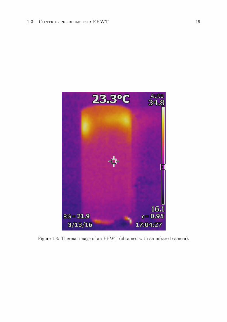
Figure 1.3: Thermal image of an EHWT (obtained with an infrared camera).
20 Chapter 1. Introduction
Heating power u(t)
Water drain
State of chargeEHWT
Figure 1.4: Input-output representation of the tank.
which prevails over electric load management. In our case, the constraints can be definedusing a comfort temperature set by the user. Water over this temperature can be blendedwith cold water, while water under the comfort temperature is useless. Additionally,functioning constraints can be considered. For instance, to prevent skin burns and EHWTmalfunctions, a maximum (safety) temperature can be defined.
The optimization problem can be defined from the electricity producer’s perspective, byassuming that we have control of the power injection u(t) = (u1(t), ..., uk(t)) of a group ofk tanks during a time period [t0, tf ]. The electricity producer usually desires to minimizea given objective function, while ensuring user’s needs. For a given tank i, the fact that astrategy ui ensures user’s comfort will be noted ui ∈ U i, U i being the set of admissiblecontrols for tank i. A most useful problem of minimization concerns the cost of heating.Given a price signal for electricity over time c(t, ·), an optimal control problem can bedefined as follows:
min(u1,...,uk)∈U1×...×Uk
∫ tf
t=t0c(t,
k∑j=1
uj(t))k∑j=1
uj(t). (P1)
We call this problem P1. In this formulation, the price depends on the total demand, sincethe whole population of EHWT is not negligible in the whole demand6.
Alternatively, the objective function can be defined as a quadratic distance to anobjective for the aggregated consumption fo(t). This gives
min(u1,...,uk)∈U1×...×Uk
∫ tf
t=t0(fo(t)−
k∑j=1
uj(t))2. (P2)
We call this problem P2. Works from the literature on these problems (or closely-relatedones) generally consider that the temperature in the tank is uniform and neglect thestratification ([DL11, SCV+13]). This assumption can lead to a violation of the comfortconstraints caused by the supply of cold or tepid water, and do not take advantage of thestratification. For this reason, we wish to have a new look at these problems, and proposenew solutions for them.
6if the considered group is small, prices appear as flat and this problem splits into k distinct problems(since the functioning constraints are readily decoupled)
minui∈Ui
∫ tf
t=t0
c(t)ui(t).
1.4. Contributions of the thesis 21
1.4 Contributions of the thesis
The thesis proposes several contributions.A first part is dedicated to representing an EHWT as an input-output system (see
Fig. 1.4). The idea is to develop a simple, numerically tractable and relatively accuratemodel that can be implemented inside a computing unit embedded in a “smart EHWT” forpractical applications of optimization strategies. In Chapter 2, a physics-based partialdifferential model including a natural convection term for the temperature is developed.Its terms are defined based on our physical understanding of the 1D dynamics in the tank.Fed with experimental recordings of data of electric consumption and water drains, themodel is able to reconstruct the temperature profile in the tank. Then, this model issimplified in Chapter 3, into a phenomenological multi-period model which distinguishesseveral functioning states. This second model is computationally cheap and accurate. Itmay be integrated into the embedded chip of a smart EHWT. In the perspective of controldesign, a realistic domestic hot water consumption model is developed in Chapter 4. It canbe used to randomly generate drain scenarios in near future, correlated with recent drainsevent. These scenarios can be used to proof-test optimal heating strategies which shouldavoid the prejudicial case of shortage of hot water. The temperature profile gives a precisedescription of the state of the EHWT, but is too heavy to be manipulated for controlpurposes. For this reason, we define three variables of interest that ease the handling ofcomfort constraints. This is the purpose of Chapter 5. This final modeling stage completesthe definition of an input-output model for the EHWT subjected to a random hot waterdemand.
The second part focuses on the design of optimal control strategies for a group of tanks.It is assumed that the individual heating elements of the tanks can each be remotely pilotedby a decision center (they are said to be controllable). Among them, upon request, afraction can compute and transmit to the decision center information on their state. Theyare said to be smart. Three use-cases are studied. Chapter 6 adresses the case of a smallnumber of smart and controllable EHWT (from 1 to 4). A discrete-time optimal resolutionmethod for problems P1 and P2 is defined. In the case of a single unit, the optimizationalgorithm can be integrated in the chip of the tank, which will automatically define itsheating strategy against an external price signal or with self-consumption objectives. InChapter 7, we focus on a medium-scale group of controllable tanks (from a few hundredsto several millions) and present a heuristic for problem P2 which keeps the heating periodundivided to minimize thermo-hydraulic hazards. This heuristic, based on the stochasticnature of the problem, uses the statistical smoothing induced by the large number of tanksto approach the objective curve. If a fraction of the group is constituted of smart tanks,results are improved and can reach almost the same performance as in the case when allthe tanks are smart (in which sub-optimality is less than 1%). Finally, the modeling ofthe behavior of a infinite population of tanks is presented in Chapter 8. This (prospective)approach aims at studying the output response of the whole group subjected to globalstrategies.
Perspectives and conclusions are discussed in Chapter 9.
Note. The works presented in this thesis have been the subject of the following publica-tions and patents.
22 List of patents
List of conference papers[BMP15a] N. Beeker, P. Malisani, and N. Petit. A distributed parameters model for
electric hot water tanks. In Proceedings of the American Control Conference,ACC, 2015.
[BMP15b] N. Beeker, P. Malisani, and N. Petit. Dynamical modeling for electric hotwater tanks. In Proceedings of the Conference on Modelling, Identification andControl of Nonlinear Systems, MICNON, 2015.
[BMP16a] N. Beeker, P. Malisani, and N. Petit. Discrete-time optimal control of electrichot water tank. In Proceedings of the 11th IFAC Symposium on Dynamics andProcess Systems, including Biosystems, DYCOPS, 2016.
[BMP16b] N. Beeker, P. Malisani, and N. Petit. Modeling populations of electric hotwater tanks with Fokker-Planck equations. In Proceedings of the 2nd IFACWorkshop on Control of Systems Governed by Partial Differential Equations,CPDE, 2016.
[BMP16c] N. Beeker, P. Malisani, and N. Petit. An optimization algorithm for load-shifting of large sets of electric hot water tanks. In Proceedings of the 25thInternational Conference on Efficiency, Cost, Optimization, Simulation andEnvironmental Impact of Energy Systems, ECOS, 2016.
[BMP16d] N. Beeker, P. Malisani, and N. Petit. Statistical properties of domestic hotwater consumption. In Proceedings of the 12th REHVA World Congress CLIMA,2016.
List of patents[BMC15a] N. Beeker, P. Malisani, and A.S. Coince. Ballon Intelligent - 1554897 (patent
applied for), 2015.
[BMC15b] N. Beeker, P. Malisani, and A.S. Coince. Ballon Intelligent - EDP - 1554898(patent applied for), 2015.
[BMC15c] N. Beeker, P. Malisani, and A.S. Coince. Ballon Intelligent - Trois zones -1554896 (patent applied for), 2015.
Introduction
La gestion de la demandeComme décrit dans de nombreuses études, la part grandissante des énergies renouve-lables dans le mix énergétique complique la gestion de l’équilibre offre-demande del’électricité [Eur11, EPMSS11]. Les sources renouvelabes peuvent s’ajouter à des moyens deproduction non-flexibles7, et provoquer des surcharges du réseau comme en témoignent lesépisodes récents de prix négatifs sur les marchés J+1 en France et en Allemagne [EPE14].Des problématiques similaires sont observées au niveau local dans la régulation de tensiondu réseau de distribution, initialement dimensionné pour acheminer de manière relative-ment stable l’électricité au consommateur, qui doit désormais supporter une productionphotovoltaïque distribuée.
Pour compenser ce déficit de flexibilité sur les moyens de production d’électricité, onpeut chercher d’autres gisements de flexibilité, notamment du cÃťté de la demande. C’estl’objet de la gestion de la demande (GD), un ensemble de techniques visant a modifierla demande des consommateurs. Le potentiel de la GD apparaît prometteur [PD11].C’est d’autant plus vrai actuellement, car la situation de surcapacité de la productiond’électricité en Europe rend la construction de moyens de production flexibles non rentableet par conséquent peu probable dans les années à venir.
Un facteur clé pour le développement de la GD est la disponibilité de capacités destockage. Pour cette raison, les gestionnaire de réseaux et les producteurs d’électricitérecherchent de nouveaux moyens de stockage. Dans ce contexte, les importants parcsde chauffe-eau Joule (CEJ) domestiques de nombreux pays8 apparaissent prometteurs,particulièrement pour le problème dominant du décalage de charge. Les principales raisonssupportant ce fait sont les qualités intrinsèques de ce stockage : la grande capacité desparcs de CEJ, leur caractère réparti sur le territoire, et leur fonctionnement.
En principe, la chauffe d’un CEJ peut être planifiée librement, par exemple en fonctiondes prix de l’électricité. Si de nombreuses politiques tarifaires ont été étudiées et élaborés,la tarification en fonction de l’heure de consommation reste dominante pour la plupart desconsommateurs, par exemple en France avec le système d’heures pleines/heures creuses9.Ces politiques définissent des plages horaires (par exemple des heures pleines de 6h à22h, et des heures creuses de 22h à 6h) pendant lesquelles un tarif prédéterminé estappliqué. Le début de ces plages étant connu, des stratégies de chauffe simples sontgénéralement appliquées à chaque CEJ. La chauffe est mise en marche immédiatement
7comme le parc nucléaire français, qui représentait 76,3% de la production nationale d’électricité en2015 [Bil15]
8la part de marché du CEJ dans les moyens de chauffe est de 35% au Canada [AWR05], de 38% auxU.S.A [RLLL10], de 45% en France [MSI13]
9les tarifications différentielles Economy 7 et Economy 10 au Royaume-Uni sont d’autres exemplestypiques
24 List of patents
après réception d’un signal analogique correspondant à la plage d’heures creuses. La chauffeest ensuite arrêtée lorsque toute l’eau du CEJ est chaude. Cette stratégie élémentairefavorise naturellement la consommation d’électricité pendant la nuit (une période pendantlaquelle les prix de marché de l’électricité sont bas), alors que l’eau chauffe est utilisée lajournée suivante. A grande échelle, le résultat est dans l’ensemble positif, mais un effetindésirable est que la consommation globale redescend rapidement à un bas niveau aumilieu de la nuit, lorsque les coûts de production de l’électricité sont les plus bas.
Cet effet négatif doit être corrigé. Le développement rapide de la domotique ouvre lavoie à des stratégies de chauffe nouvelles sur de grands parcs de CEJ, qui peuvent s’avéreravantageuses à la fois pour les consommateurs et pour les producteurs d’électricité [Lan96].Cette thèse présente des travaux développés dans cette perspective, et vise à développerdes méthodes qui pourraient être intégrées à des “CEJ intelligents” mettant en œuvre detelles stratégies.
Fonctionnement et modèles de CEJUn CEJ prend usuellement la forme d’un ballon cylindrique vertical, rempli d’eau. Unerésistance chauffante10 est plongée dans le bas du ballon (voir Fig. 1.5).
La résistance est longiligne et relativement et relativement grande (elle couvre jusqu’àun tiers de la longueur du ballon). Lorsque l’utilisateur soutire de l’eau, cette eau estprélevée dans le haut du ballon pendant que de l’eau froide est injectée dans le bas duballon au même débit (sous l’effet de l’équilibre de pression du réseau de distributiond’eau), de telle sorte que le ballon est toujours plein.
Dans la littérature [Bla10, KBK93, ZLG91], les réservoirs d’eau chaude sont modéliséscomme des colonnes verticales, régi par des phénomènes thermo-hydrauliques : diffusionthermique, effets de flottabilité dus à la variation de densité de l’eau en fonction de satempérature et des mélanges qu’ils engendrent, convection due au soutirage et mélangeengendré, et enfin pertes thermiques vers l’extérieur. Dans le ballon, des couches d’eaude températures différentes coexistent (voir Fig. 5.1 et Fig. 1.7). Au repos, ces couchesne sont affectées que par la diffusion thermique, dont les effets sont relativement lentscomparés aux autres phénomènes [HWD09].
Le fait qu’un profil (croissant) de température dans le ballon, non uniforme, restedans un quasi-équilibre est appelé phénomène de stratification [DR10, HWD09, LT77].En pratique, cet effet est utile pour l’utilisateur, car l’eau chaude disponible pour laconsommation est naturellement stockée près de l’évacuation du CEJ, pendant que le restedu ballon est chauffé (voir Fig. 1.6). La zone de fort gradient de température entre l’eauchaude et l’eau froide (voir Fig. 1.6) est appelée thermocline [ZLG91]. En pratique, laconsommation d’eau chaude prend la forme d’une succession de soutirages d’amplitudesvariables, correspondant aux usages du consommateur (douche, bain, hygiène, cuisine). Ladurée de ces soutirages est courte à l’échelle de la journée, et les moments où ils ont lieu nesont pas fixés, mais inhérents au caractère stochastique du comportement de l’utilisateur.
La plupart des stratégies de contrôle de parcs de CEJ ne prennent pas en compte lastratification et supposent simplement que la température dans le ballon est uniforme [DL11,SCV+13]. Cette approche est pertinente pour les ballons de petites tailles, mais ne permetpas de valoriser le phénomène de stratification. Comme il sera exposé dans cette thèse,inclure un modèle de stratification dans ces stratégies peut permettre des améliorations
10ou un ensemble de plusieurs résistances rapprochées
List of patents 25
capteurs detempérature
isolation
thermostat
résistanceschauffantes
eau chaudeeau froide
Figure 1.5: Schéma simplifié d’un CEJ. Les capteurs de température ajoutés pour lesmesures expérimentale ont été représentés, ils ne sont pas présents sur les CEJ du commerce.
26 List of patents
Temperature
Eau froide Thermocline Eau chaude h0
Tmax
Tin
x
Figure 1.6: Exemple de profil de température à l’intérieur d’un ballon stratifié.
non négligeables des performances.
Dans la littÃľrature, les premiers modèles de ballon incluant la stratification se sontintéressÃľs à des réservoirs de grande taille dans les sous-sols des bâtiments utilisés pourle chauffage ou la climatisation [OGM86]. Ces réservoirs n’incluent pas de résistancechauffante ou de système de réfrigération direct. Ils sont simplement utilisés pour stockerde grandes quantités d’eau chauffée ou refroidie par d’autres moyens. La plupart desauteurs utilisent la symétrie de révolution du système et le fait que l’écoulement estprincipalement vertical (en raison de la géométrie du système). La température du ballonest alors supposée homogène pour une hauteur donnée, et l’étude est limitée à des modèlesunidimensionnels de différentes natures : équations aux dérivées partielles de convection-diffusion [OGM86, ZGM88], modèles par couches [HWD09], modèles piston [KBK93]. Lestravaux les plus récents comprennent des élements chauffants, comme des échangeursthermiques dans les chauffe-eau solaires ou thermodynamiques [SFNP06, Bla10]. Desmodèles tri- ou bidimensionnels (en utilisant la symétrie de révolution), souvent discrétiséspour des objectifs de simulations numérique (comme par exemple de mécanique des fluidesnumérique) [Bla10, HWD09, JFAR05], ou des modèles dits zonaux basés sur le logicielTRNSYS [JFAR05, KBM10] sont l’objet de certaines Ãľtudes. Ces modèles, bien queprécis, sont coûteux numériquement et principalement utilisés dans la conception optimale(hors ligne) des échangeurs et des tuyaux dans les chauffe-eau les plus récents.
Un arbitrage entre précision et complexité doit être établi pour reproduire les phénomènesphysiques observés en pratique, tout en permettant le calcul rapide de stratégies optimisées.Dans cette optique, les modèles unidimensionnels apparaissent comme le niveau idéal decomplexité. Les travaux de modélisation et de contrôle de cette thèse se limiteront à cecas.
List of patents 27
Figure 1.7: Image thermique d’un CEJ (obtenue à l’aide d’une caméra infrarouge).
28 List of patents
Puissance de chauffe u(t)
Soutirage
Etat de chargeCEJ
Figure 1.8: Représentation entrée-sortie d’un CEJ.
Problèmes de contrôle pour les parcs de CEJEn principe, un CEJ peut être vu comme un système dynamique a deux entrées et unesortie (voir Fig. 1.8). Les deux entrées sont i) la puissance de chauffe (qui est une variablede contrôle) et ii) le débit d’eau sortant soutiré par l’utilisateur. L’état interne est le profilde température de l’eau dans le ballon, qui peut être utilisé pour définir, dans un butd’optimisation, des indices de performances (sorties). Ces sorties peuvent (pour l’instantapproximativement ) être définies comme l’état de charge du CEJ. Comme on le verradans cette thèse, une définition plus précise est nécessaire.
Du point de vue de l’optimisation, la satisfaction de l’utilisateur est une contrainte,qui prévaut sur la gestion de la charge électrique. Dans notre cas, les contraintes peuventêtre définies en utilisant une température de confort réglée par l’utilisateur. L’eau audessus de cette température peut être mitigée, en la mélangeant avec de l’eau froide, alorsque l’eau en dessous de la température de confort est inutile. De plus, des contraintes defonctionnement sont a prendre en compte. Par exemple, pour éviter des brûlures cutanéesou des dysfonctionnements du CEJ, une température maximum (de sécurité) peut-êtredéfinie.
Le problème d’optimisation peut être défini du point de vue du producteur, en supposantqu’on dispose du contrôle de l’injection de puissance u(t) = (u1(t), ..., uk(t)) d’un parc dek ballons pendant une période [t0, tf ]. Le producteur d’électricité souhaite généralementminimiser une certaine fonction objectif, toute en satisfaisant les contraintes de l’utilisateur.Pour un ballon donné i, le fait qu’une stratégie ui garantisse le confort de l’utilisateur seranoté ui ∈ U i, U i étant l’ensemble des contrôles admissibles pour le ballon i. Un problèmeimportant de minimisation concerne le coût de la chauffe. Étant donné un signal prix pourl’électricité au cours du temps c(t, ·), un problème de contrôle optimal peut être définicomme
min(u1,...,uk)∈U1×...×Uk
∫ tf
t=t0c(t,
k∑j=1
uj(t))k∑j=1
uj(t). (P1)
On appelle ce problème P1. Dans cette formulation, le prix dépend de la consommationtotale en électricité, dans la mesure ou la taille des parcs de CEJ n’est pas négligeabledans la demande globale11.
11si le groupe considéré est de petite taille, étant donné que les contraintes de fonctionnement sontdécouplées, les prix apparaissent comme plats et ce problème se décompose en k problèmes distincts
minui∈Ui
∫ tf
t=t0
c(t)ui(t).
List of patents 29
Alternativement, la fonction objectif peut-être définie comme une distance quadratiqueà un objectif pour la consommation agrégée fo(t). Le problème est alors
min(u1,...,uk)∈U1×...×Uk
∫ tf
t=t0(fo(t)−
k∑j=1
uj(t))2. (P2)
On appelle ce problème P2. Les travaux trouvés dans la littérature sur ce type de problèmessupposent généralement que la température est uniforme dans le ballon et négligent lastratification [DL11, SCV+13]. Cette hypothèse peut mener à une violation des contraintesde confort en délivrant de l’eau froide ou tiède, et ne valorise pas la stratification. Pourcette raison, nous souhaitons porter un nouveau regard sur ces problèmes, et proposer dessolutions alternatives.
Contributions de la thèseCette thèse propose plusieurs contributions.
Une première partie est dédiée à la représentation d’un CEJ en tant que systèmeentrée-sortie (voir Fig. 1.8). L’idée est de développer un modèle simple, adaptable et assezprécis, qui puisse être utilisé dans une unité de calcul embarquée dans un CEJ intelligentpour l’application pratique des stratégies d’optimisations. Dans le chapitre 2, un modèlephysique prenant la forme d’un système d’équations aux dérivées partielles est développé,incluant notamment un terme de convection naturelle. Les termes du modèles sont baséssur notre compréhension physique de la dynamique 1D dans le ballon. Validé par desdonnées expérimentales liées à des chroniques de soutirage et de consommation électrique,le modèle se montre capable de reconstruire le profil de température Ãă l’intérieur d’unballon. Dans un second temps, ce modèle est simplifié dans le chapitre 3 en un modèlephénoménologique multi-périodes qui distingue plusieurs états de fonctionnement. Cesecond modèle est précis et peu coûteux numériquement. Il est possible de l’intégrer dansun calculateur embarqué dans un CEJ intelligent. Dans la perspective de la conceptiondes stratégies de contrôle, un modèle réaliste de consommation d’eau chaude sanitaire estdéveloppé dans le chapitre 4. Il peut être utilisé pour générer aléatoirement des scénarios desoutirages dans le futur proche, corrélé avec l’historique récent de soutirage. Ces scénariospeuvent être utilisés pour mettre à l’épreuve des stratégies de chauffe optimale et vérifierqu’elles ne génèrent pas une pénurie d’eau chaude. Le profil de température offre unedescription précise de l’état du CEJ, mais son caractère distribué le rend trop lourd pourêtre manipulé dans un but de contrôle. Pour cette raison, on définit trois variables d’intérêtqui facilitent la manipulation des contraintes de confort. C’est l’objet du chapitre 5. Cetteétape finale de modélisation termine la définition d’un modèle entrée-sortie pour un CEJsoumis à une demande d’eau chaude sanitaire aléatoire.
La seconde partie de la thèse s’intéresse à la conception de stratégies de contrôleoptimal pour un parc de CEJ. On suppose que la chauffe de chaque ballon peut être pilotéeà distance par un centre de décision (les ballons étant dits contrôlables). Parmi eux, unepartie peut calculer et transmettre sur demande au centre de décision des informationssur leurs états. Ces ballons sont dits intelligents. Trois cas de figure sont étudiés. Lechapitre 6 s’intéresse aux cas d’un petit nombre de ballons contrôlables et intelligents (de1 à 4). Une méthode de résolution optimale en temps discret pour P1 et P2 y est définie.Dans le cas d’un ballon unique, l’algorithme d’optimisation peut être intégré dans lecalculateur embarqué du ballon, et définit automatiquement sa stratégie de chauffe future
30 Liste des brevets
en utilisant par exemple un signal prix extérieur ou des objectifs d’auto-consommation.Dans le chapitre 7, on étudie des parcs de tailles intermédiaires (de quelles centaines àplusieurs millions). On propose une heuristique de résolution du problème P2, gardantles périodes de chauffes indivisées pour minimiser les aléas thermo-hydrauliques. Cetteheuristique repose sur la nature stochastique du problème, et utilise le lissage statistiquenaturel généré par le grand nombre de ballons pour se rapprocher de la courbe objectif. Siune partie des ballons est contrôlable et intelligente, les résultats s’améliorent et la perted’optimalité peut descendre à moins de 1%. Enfin, un modèle de comportement d’un parcinfini de ballons est proposé dans le chapitre 8. Cette approche (prospective) vise à étudierla réaction d’un parc soumis à des stratégies d’ensemble.
Le chapitre 9 est consacré à la conclusion, et à la présentation de perspectives.
Note. Les travaux présentés dans cette thèse ont été l’objet des publications et brevetssuivants.
Liste des papiers de conférence[BMP15a] N. Beeker, P. Malisani, and N. Petit. A distributed parameters model for
electric hot water tanks. In Proceedings of the American Control Conference,ACC, 2015.
[BMP15b] N. Beeker, P. Malisani, and N. Petit. Dynamical modeling for electric hotwater tanks. In Proceedings of the Conference on Modelling, Identification andControl of Nonlinear Systems, MICNON, 2015.
[BMP16a] N. Beeker, P. Malisani, and N. Petit. Discrete-time optimal control of electrichot water tank. In Proceedings of the 11th IFAC Symposium on Dynamics andProcess Systems, including Biosystems, DYCOPS, 2016.
[BMP16b] N. Beeker, P. Malisani, and N. Petit. Modeling populations of electric hotwater tanks with Fokker-Planck equations. In Proceedings of the 2nd IFACWorkshop on Control of Systems Governed by Partial Differential Equations,CPDE, 2016.
[BMP16c] N. Beeker, P. Malisani, and N. Petit. An optimization algorithm for load-shifting of large sets of electric hot water tanks. In Proceedings of the 25thInternational Conference on Efficiency, Cost, Optimization, Simulation andEnvironmental Impact of Energy Systems, ECOS, 2016.
[BMP16d] N. Beeker, P. Malisani, and N. Petit. Statistical properties of domestic hotwater consumption. In Proceedings of the 12th REHVA World Congress CLIMA,2016.
Liste des brevets[BMC15a] N. Beeker, P. Malisani, and A.S. Coince. Ballon Intelligent - 1554897 (patent
applied for), 2015.
[BMC15b] N. Beeker, P. Malisani, and A.S. Coince. Ballon Intelligent - EDP - 1554898(patent applied for), 2015.
Liste des brevets 31
[BMC15c] N. Beeker, P. Malisani, and A.S. Coince. Ballon Intelligent - Trois zones -1554896 (patent applied for), 2015.
Part I
The EHWT : behaviour andproposed representation
Chapter 2
A physics-based representation ofEHWT
Un modèle physique pour les CEJ. Dans ce chapitre, nous présentons un modèle deCEJ prenant la forme d’un système couplé de deux equations aux dérivées partielles, suivide simulations et d’une validation expérimentale. Le modèle permet de reproduire le profilde température dans le ballon au cours du temps.
In this chapter, we develop a distributed parameter model for the dynamics of thetemperature profile in an EHWT. The microscopic and macroscopic effects observed inresponse to the water drain and the power injected in the tank take central roles in thismodel.
The model can be seen as an extension of existing one-dimensional convection-diffusion linear equations modeling the draining convection and mixing originally developedin [OGM86, ZGM88, ZLG91] in the general context of storage tanks. In details, to theclassic governing equation already found in the previously cited works, we add a nonlinearvelocity term stemming from an empirical law representing turbulent natural convectioncaused by heating, and we explicitly include heating power as a source term1.
The model we develop is shown to be in accordance with experimental data presentedin this chapter. These data clearly stress the following: i) heating water with an EHWTtakes time, ii) during the heating process, a zone of uniform temperature appears andgrows until it covers the whole tank, iii) draining induces a piston flow, and also causessome internal mixing which is non negligible. As will be shown, the proposed distributedparameter model is able to reproduce these observations.
The chapter is organized as follows. After having described the proposed model inSection 2.1, we illustrate it by means of simulations and compare it against experimentaldata in Section 2.2. A summary is given in Section 2.3.
1This model enrichment can be related to the numerics oriented works of [VKA12] who proposes toconsider an additional natural convection term in the finite difference scheme discretizing a one-dimensionalconvection-diffusion equation.
36 Chapter 2. A physics-based representation of EHWT
2.1 PDE for heating and draining
2.1.1 Draining model as a PDETo emphasize the effects of stratification, our model solely uses one-dimensional partialdifferential equations. The works of Zurigat on draining effects in stratified thermal storagetanks [ZGM88, ZLG91] serves as baseline. The novelty is to introduce the heating system.It is treated in § 2.1.2 and § 2.1.3. The equation below accounts for draining and itsinduced turbulent mixing effects. It is an usual one-dimensional energy balance where theturbulence is lumped into a diffusion term
∂tT + ∂x(vdT ) = (αth + αd)∂xxT .In this equation, T (x, t) is the temperature at time t and height x, vd ≥ 0 is the
velocity induced by the draining (assumed to be spatially uniform but time-varying), αthis the thermal diffusivity and αd is an additional turbulent diffusivity term representingthe mixing effects. Zurigat [ZGM88, ZLG91] considers the same equation and introducesthe ratio εd = αth+αd
αth. An experimental correlation is shown with the Reynolds number
and the Richardson number Ri in the tank2 defined as
Ri = gαV (Tin − Ta)Lcv2d
(2.1)
where g is the gravitational acceleration, αV is the volumetric coefficient of thermalexpansion of the fluid (here water), Tin is the temperature of the inlet water, Ta is theambient temperature and Lc is a characteristic vertical length3. This correlation can beused in our case.
A heat losses term (to the exterior of the tank assumed to be at temperature Ta) canbe added to this equation. Then, one obtains
∂tT + ∂x(vdT ) = εdαth∂xxT − k(T − Ta) (2.2)
where the factor k is defined byk = UhΠ
Sρcp
where ρ is the density of water, cp its specific heat capacity, Uh is the overall heat transfercoefficient based on the tank internal surface area, Π is the tank internal perimeter and Sits effective cross-section.
Note h the vertical length of the tank internal volume. Equation (2.2) is assumed tohold over Ω× I, where I =]t0, tf ] is a time interval and Ω =]0, h[. Classically, we considerboundary conditions of the Robin [DL93] form vd(T (0, t) − Tin) + εdαth∂xT (0, t) = 0at x = 0, and of the Neumann [DL93] form ∂xT (h, t) = 0 in x = h, meaning that energyis allowed to leave the system with the outlet flow but not with diffusion.
2.1.2 Including heating and buoyancy forcesEquation (2.2) integrates the most obvious phenomena taking place in an EHWT. Theeffects of heating are of two types: direct and indirect. The direct effect is a source term
2The Richardson number (2.1) is a dimensionless number representing the relative importance ofnatural convection compared to forced convection [ZLG91]
3This correlation is influenced by the geometry of the inlet nozzle [IFYLG14, ZLG91]
2.1. PDE for heating and draining 37
Figure 2.1: Plumes of turbulent natural convection over an exchanger, from [Bla10].
in the balance equation. The indirect effect is buoyancy. It can be added in the model atthe expense of linearity, as is described below.
When the heating system is on, temperature of water around the heating elementstarts to rise. By buoyancy, hot water replaces colder water above by a phenomenon calledRayleigh-Bénard convection [Pet07, Gau08, Gib07]. This convection can take variousforms depending on the characteristics of the system, represented by the Rayleigh number
Ra = gαV (Ts − T∞)L3c
ναth
where ν is the kinematic viscosity of the fluid, Ts is the temperature of the surface (herethe heating element), and T∞ is the temperature in the tank far from it. This adimensionalnumber scales the effects of buoyancy and conduction: if it is low, the conduction will bethe main heat transfer factor, if it is high, the natural convection will predominate. Overa critical value (Ra = 1108 for [Pet07], Ra = 3, 5 · 104 for [Gau08]), turbulent naturalconvection appears under the form of a pattern of plumes forming convection cells calledBénard cells which can take various forms and sizes.
For any EHWT found in households, even with a small Ts−T∞ difference, the Rayleighnumber is far over the critical value, and plumes of turbulent water appears over theheating system (see Fig. 2.1 reproduced from [Bla10]). Therefore, convection dominatesconduction. To include this effect into (2.2), we simply consider that, at each given height,two distinct temperatures co-exist in the convection cells. Then, to our equation on T , weappend an interacting equation bearing on a new physical quantity ∆T (x, t) representingthe temperature spread at each height x over T . This gives the following system
38 Chapter 2. A physics-based representation of EHWT
In the two equations above, three terms have been added: a velocity term vnc ofnatural convection, which is responsible for transport of energy in the system, a heatexchange term Φ(x, t)∆T (x, t) (representing at each height the mixing induced by naturalconvection being proportional to the temperature spread), and the spatially distributedsource term PW (representing the power injected in the tank all along the element, generallyfrom the bottom of the tank to one third of its height), which drives the dynamic of ∆T .The boundary conditions for (2.3) remain unchanged, while the boundary conditionsfor (2.4), as a temperature spread, are vd∆T (0, t) + εdαth∂x(∆T )(0, t) = 0 at x = 0and ∂x(∆T )(h, t) = 0 at x = h.
2.1.3 Model for natural convection and internal heat transferWe now introduce a model for the transport velocity appearing in (2.4). This veloc-ity vnc(x, t) is non-constant. It is non-zero at a given altitude x only if there exists colderwater over the height x (i.e. downstream). We give to vnc the following integral form
vnc(x, t) = v(∫ h
x[T (x, t) + ∆T (y, t)− T (y, t)]ζ+dy)ξ (2.5)
where [z]+ is the positive part of z and v is a positive factor, and where 0 < ζ < 1 and0 < ξ < 1 are tuning parameters the value of which are chosen to fit experimental data.These parameters reduce the impact of the downstream temperatures differences andsmooth the velocity when it is nonzero. The exchange coefficient Φ between the twoequations is also non-constant and we model it as
Φ(x, t) = φ[vmax − vnc(x, t)]+ (2.6)
where φ and vmax are two tuning parameters. The rationale behind this expression is thatthe horizontal mixing is stronger when the natural convection flow reaches the upper partof the tank and has a lower speed.
2.1.4 Summary of the modelAccording to the previous discussion, the EHWT can be represented by two distributedstate variables, T and ∆T , governed by (2.3) and (2.4). In those governing equationstwo velocities appear: vd which is spatially uniform and is equal to the output flowrate(drain) of the system, and vnc which is defined in (2.5) to model the effects of naturalconvection. Heat is injected into the system through a distributed source term PW and theheat exchange between the two equations is proportional to ∆T with a coefficient (variablein space) defined in (2.6). Finally, αth, εd, k, v, ζ, ξ, φ and vmax are constant parametersdepending on physical constants and the geometry of the tank. Typical values for theEHWT defined in Table 2.1 are given in Table 2.2. They result from an identificationprocedure.
2.2 Model validation
2.2.1 Experimental setupTo validate the model, experiments have been conducted in the facilities of EDF LabResearch Center, on an Atlantis ATLANTIC VMRSEL 200L water tank. The power
2.2. Model validation 39
is injected via three nearby elements permitting a power injection up to 2200W. Thedimensions of the water tank are specified in Table 2.1.
Volume L 200Length m 1.37Maximal power W 2200Heat losses coefficient W·m−2K−1 0.66
Table 2.1: Specifications of the EHWT used in experiments.
αth m2s−1 1.43 · 10−7
εd - 13k s−1 1.43 · 10− 6v m1−ξ·s−1K−ζξ 10−3
ζ - 0.2ξ - 0.5φ m−1 0.03vmax ms−1 0.35
Table 2.2: Parameters of the model for the associated EHWT.
The water tank has been equipped with internal temperature sensors recording temper-ature at 15 locations of different heights, 15 cm deep inside the water tank (see Fig. 1.1).This depth is sufficient to bypass the insulation of the tank. It is assumed that the sensorshave no effect on the flows (e.g. that they do not induce significant drag). Besides, thefollowing quantities have been recorded with external sensors: injected power, water flowat the inlet, water temperature at the inlet. These three quantities feed the model, theoutput of which can be compared with the temperature measured by the sensors. Thecomparisons are directed into an optimization procedure identifying the coefficients givenin Table 2.2. Conducted experiments took the form of fourteen 24 h runs with a samplingrate of 1Hz. Histories for drain are taken from the normative sheets emitted by the Frenchnorm organism [NF 11] for a tank of such capacity, associated with a classical night-timeheating policy until total load. Subsequent experiments consider similar total consumptionbut with different drain/heat combinations and overlaps to test the model under varioussituations.
2.2.2 ResultsFor sake of illustration, several operating conditions are reported next. Simulations havebeen conducted on a quad-core Intel Core i7-4712HQ processor equipped with 16Goof memory. Numerically, this system of equations can be solved with finite differenceschemes. We use a Crank-Nicholson scheme (see [All07]) for the diffusive term, andan upwind scheme for the convective part. The later is stable only conditionally to aCourant-Friedrichs-Lewy condition [All07]. In our case, due to the non-linear nature ofvnc, short time-steps must be chosen. In turn, this increases the computational load whichis already high due to the evaluation of the integral appearing in vnc, for each space-step.This can lead to long computation times (see Table 2.3). Fig. 2.2 (a) shows the variation
40 Chapter 2. A physics-based representation of EHWT
0 20 40 60 80 100
20
30
40
50
60
70
80
H e ig h t (% o f m a x .)
Tem
perature(oC)
0 20 40 60 80 100
20
30
40
50
60
70
80
H e ig h t (% o f m a x .)
Tem
perature(oC)
(a.1) (b.1)
0 20 40 60 80 100
20
30
40
50
60
70
80
H e ig h t (% o f m a x .)
Tem
perature(oC)
0 20 40 60 80 100
20
30
40
50
60
70
80
H e ig h t (% o f m a x .)
Tem
perature(oC)
(a.2) (b.2)
0 20 40 60 80 100
20
30
40
50
60
70
80
H e ig h t (% o f m a x .)
Tem
perature(oC)
0 20 40 60 80 100
20
30
40
50
60
70
80
H e ig h t (% o f m a x .)
Tem
perature(oC)
(a.3) (b.3)
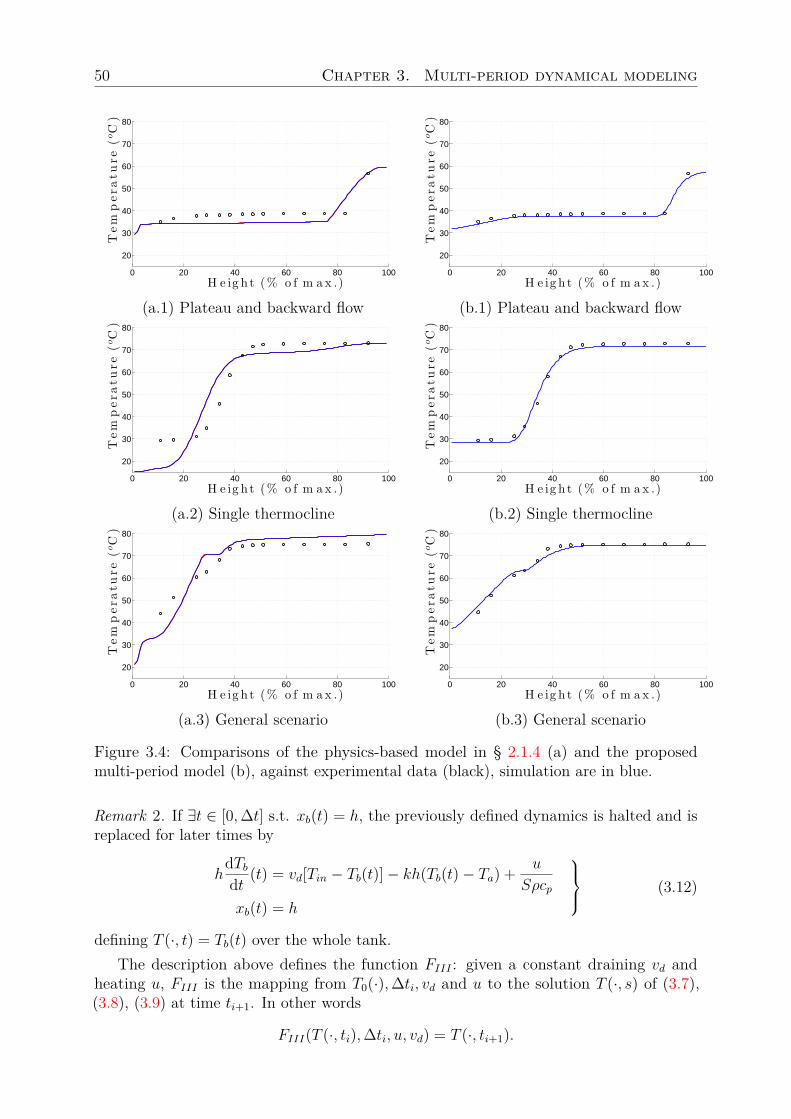
Figure 2.2: Variations of the temperature profile during a heating period (a) and during adraining period (b) (blue: model prediction, black: experimental values).
of the temperature during a heating period for a tank initially completely cold. Fig. 2.2(b) shows the response to draining of a heated tank. The results are quite satisfactory.Some mismatch appears in the lower part of the tank during draining, and in upper partsduring heating. They can be due to the chosen one-dimensional representation, since theneglected effects of radial inhomogeneity may be stronger near the ends of the tank, and tosome mixing effects that have not be taken into account. However, the results show thatthe model is accurate enough, even in 24 h open-loop runs. To support this statement, thedistribution of the absolute difference between experimental value and model prediction isgiven in Table 2.3 (produced over the whole set of data).
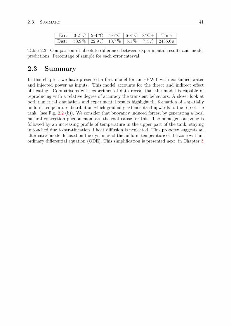
Table 2.3: Comparison of absolute difference between experimental results and modelpredictions. Percentage of sample for each error interval.
2.3 SummaryIn this chapter, we have presented a first model for an EHWT with consumed waterand injected power as inputs. This model accounts for the direct and indirect effectof heating. Comparisons with experimental data reveal that the model is capable ofreproducing with a relative degree of accuracy the transient behaviors. A closer look atboth numerical simulations and experimental results highlight the formation of a spatiallyuniform temperature distribution which gradually extends itself upwards to the top of thetank (see Fig. 2.2 (b)). We consider that buoyancy induced forces, by generating a localnatural convection phenomenon, are the root cause for this. The homogeneous zone isfollowed by an increasing profile of temperature in the upper part of the tank, stayinguntouched due to stratification if heat diffusion is neglected. This property suggests analternative model focused on the dynamics of the uniform temperature of the zone with anordinary differential equation (ODE). This simplification is presented next, in Chapter 3.
Chapter 3
Multi-period dynamical modeling forelectric hot water tank
Modèlisation dynamique multi-periode des CEJ. Dans ce chapitre, nous simplifionsle modèle précédent en distinguant trois régimes de fonctionnement. Pour chaque régime,la dynamique est décrite sous la forme d’une equation aux dérivées partielles ou auxdérivées ordinaires. La présentation du modèle est suivie d’une validation expérimentale.
The physics-based model presented earlier in Chapter 2 is concise and relativelysatisfactory. However, the accuracy, and, above all, the computational cost associated toits numerical resolution can be seen as strong limitations if one desires to embed it in a“smart EHWT”. In this chapter, we decouple heating and draining effects and develop anew model, based on the decomposition of the dynamics according to the dominant effectat stake. We distinguish three phases (periods): heating, draining and rest.
For heating, we reproduce the behavior observed earlier in the experimental datain which the temperature increases first at the bottom of the tank forming a spatiallyuniform temperature distribution which gradually extends itself upwards to the top of thetank. This homogeneous zone is followed by an increasing profile of temperature in theupper part of the tank, remaining untouched due to stratification (heat diffusion beingneglected in this case). As previously, draining is treated as a convection parameter andits associated mixing effects are reproduced by a diffusion term. However, combined tothe convection-diffusion equation, we model the effects of the water nozzle which creates amixing zone of varying temperature and volume. The cascade represents a typical Stefanproblem [FP77a, FP77b]. Finally, rest phases are simply driven by diffusion and losses.Sequencing the three phases constitutes a multi-period model. This multi-period model isthe main contribution of this chapter.
The chapter is organized as follows. Preliminary observations are displayed in Sec-tion 3.1. Section 3.2 is dedicated to the presentation of the multi-period model which is themain contribution of the chapter. Comparative studies reported in Section 3.3 concludethat this multi-period model is more accurate and more computationally efficient than thephysics-based model presented in Chapter 2. A summary is given in Section 3.4.
44 Chapter 3. Multi-period dynamical modeling
3.1 Preliminary observationsThe comparison of the physics-based model of § 2.1.4 against experimental data is overallsatisfactory even in 24 h open-loop runs, but close-up inspections have revealed somepossibilities of improvement. We now detail these.
Firstly, numerical results of this model and experimental data concur and clearly show,during heating, the creation of a temperature “plateau” starting from the bottom of thetank (see Fig. 3.4 (a.1)). In numerical simulations, this plateau has increasing temperatureand length as heating goes on, but leaves temperatures at greater heights untouched andonly progressively covers the whole of the tank. This phenomena is seen in experimentaldata in the exact same way at the exception of a small temperature backward flow observedin the highest region of plateau (see Fig. 3.4 (a.1)). These observations support the validityof the model, but they also suggest some simplifications could be performed.
Secondly, a mismatch appears during draining in the lower part of the tank. Thismismatch consists of an underestimation of the injected water temperature and a shiftof the location of the thermocline (see Fig. 3.4 (a.2)). It is believed that the mismatcharises from a local mixing in the bottom of the tank, such as the one coming from a strongsquirt out of the water injection nozzle. In turn, the dynamics of such mixing and itseffect on the thermocline location have a strong effect on the temperature profile thatcannot be easily reproduced by the simple convection-diffusion equation in a fixed domain.Accounting for them calls for a transformation of the fixed domain into a time-dependentone and an adaptation of boundary conditions.
In practice, it appears that draining and heating effects on the tank are mostly takingplace over disjoint periods. Therefore, the time interval during which the system isconsidered can be split into distinct subintervals, or periods. Introducing distinct dynamicsfor each period offers the double advantage of reducing the computational burden (enablingtailoring numerical schemes for each dynamics) and of bringing significantly improvedflexibility compared to a single system of PDE.
We now present the multi-period model we propose.
3.2 Multi-period model for heating, draining and heatlosses
3.2.1 Separations into non overlapping periodsConsider an initial time t0, an initial temperature profile T0(x), and a time tf at whichone wants to determine the temperature profile T (·, tf ). On [t0, tf ], the tank is submittedto draining and heating, characterized by the draining velocity vd(t) and the injectedpower u(t) (related to the previously defined PW via the relation u(t) =
∫ h0 PW (y, t)dy).
We assume that vd and u are piecewise constant and left-continuous (at each discontinuitypoint).
Let us define T u = (tu0 = t0, ..., tumu
= tf ) and T v = (tv0 = t0, ..., tvmv
= tf ) the sequenceof discontinuity points respectively of u and vd, and T = T u∪T v = (t0, ..., tm) the sequenceof discontinuity points of u and vd, such that t0 < t1 < ... < tm = tf . This sequence Tdefines a succession of m time intervals ]ti, ti+1] of length ∆ti. In each time interval, thetank is in one (and only one) of the phases I, II, IIIa, IIIb defined below. Over each timeinterval, u(t) and vd(t) are constant (as illustrated in Fig. 3.1).
3.2. Multi-period model for heating, draining and heat losses 45
Drainingvd(t) = 0 vd(t) > 0
Heating u(t) = 0 I IIIau(t) > 0 II IIIb
Draining velocity vd (m · s−1)
Heating power u (W )
Configuration
Time
Time
Time
tv0
t0
umax
I I II IIIIIa IIIa IIIb IIIb II
t1 t2 t3 t4 t5 t6 t7 t8 t9 = tf
tv1 tv2 tv3 tv4 tv5 tv6 tv8 = tf
tu1 tu2 = tftu0
tv7
Figure 3.1: Definition of the timeline.
Over each interval ]ti, ti+1], we desire to determine the temperature profile as a functionof time, in particular at final time ti+1. The profile at the end of a phase serves as initialcondition for the following phase. Three functions FI , FII , FIII (accounting for both IIIaand IIIb) map an initial profile and working conditions to temperature profiles for futuretimes. We note,
• T (·, ti+1) = FI(T (·, ti),∆ti)
• T (·, ti+1) = FII(T (·, ti),∆ti, u)
• T (·, ti+1) = FIII(T (·, ti),∆ti, vd, u).
Clearly, if one wishes to compute the temperature profile at any time of interest tf ,one only needs to compute the sequence of intermediate profiles T (·, ti), i = 1, ...,m− 1 asa function of the previous ones by a chain rule. Note that for the computation on a shortinterval [t0, tf ] (e.g. if one considers a succession of nearby times of interest), T can bereduced to a short list of events. Interestingly, a comparable split is developed in [KBM08]for the case of a water storage tank with external heating.
We now detail these mappings, for any index i.
3.2.2 Phase I: RestIn this part, we consider periods without any draining or heating.
46 Chapter 3. Multi-period dynamical modeling
Physical considerations
The only phenomena driving the temperature profile are diffusion and heat losses.
Dynamics
The input variables of FI are the initial profile, say T0(·), and the duration ∆ti. Theyserve in the following diffusion-heat losses one-dimensional system:
∂tT = αth∂xxT − k(T − Ta) on Ω× I∂xT (0, t) = 0 on I∂xT (h, t) = 0 on IT (x, 0) = T0(x) on Ω
(3.1)
where I =]0,∆t] and Ω = [0, h].We have FI(T (·, ti),∆ti) = T (·, ti+1).
Numerical considerations
Numerically, this system can be solved relatively easily with finite difference schemes. Weuse a Crank-Nicholson scheme [All07] on a linearly spaced mesh.
3.2.3 Phase II: HeatingPhysical considerations
Heating modeling can be simplified thanks to the plateau discussed earlier. Turbulencegenerated by buoyancy effects during the heating process is the cause of a local mixing.Here, we consider that this mixing is perfect on the plateau which is an area [0, xp(t)], andthat the buoyancy effects do not affect stratification in heights above xp(t). For sake ofsimplicity of presentation, only the case without heat losses is exposed here, but losses canbe included without too much difficulty (this is actually done for the simulation presentedin Section 3.3). To simplify the dynamics, the diffusion phenomena have to be neglected.Then, the governing equations take the form of an ODE that we derive below.
Dynamics
The input variables of FII are the initial profile T0(·), the duration ∆ti, and the constantvalue u of the heating power. The plateau temperature is noted Tp(t). It is related to xp(t)by the equation
Tp(t) = T0(xp(t)) (3.2)
corresponding to the continuity assumption at the interface between the plateau and the(untouched) initial profile (see Fig. 3.2).
An energy balance (illustrated in Fig. 3.2) gives
Tp(t)xp(t) =∫ xp(t)
0T0(x)dx+
∫ t
0
u(s)Sρcp
ds. (3.3)
Denoting T ′0 the derivative of T0, relations (3.2) and (3.3) yield the dynamics of xp(t)
3.2. Multi-period model for heating, draining and heat losses 47
Temperature
0
Height
h
Tp(t)
T0(x)
Injected energy
xp(t)
Energy initially present
Figure 3.2: Energy balance for the integral form heating model.
dxpdt = u
SρcpxpT ′0(xp), xp(0) = 0, t ∈]0,∆t] (3.4)
which directly gives Tp(t) using (3.2).For completeness, other phenomena can be included:• Heat losses at walls (with losses coefficient k) is a local phenomena that does not
alter the shape of a plateau. Its effects are some decrease of T0(·) towards ambienttemperature Ta in the form of a exponential factor e−kt of the initial profile and aadditional term in the dynamics of xp(t).
• If the plateau is not exactly uniform but a trend can be observed (for instancerepeatable variations around the heating elements), one can separate the temperatureof the plateau in two components with distinct arguments Tp(x, t) = Tpt(t) + Tpx(x)and then study the dynamics of Tpt(t).
• Finally, the small backward energy flow that is always observed (see Fig. 3.4 (a.1)) atthe interface (in a stronger way at the top of the tank) can be modeled by relaxingthe continuity hypothesis (3.2) and replacing it with
Tp(xp(t), t) + Tp∆(xp(t)) = T0(xp(t)) (3.5)where the continuity gap Tp∆ depends on the geometry of the tank (and has to beidentified).
Integration of such optimal features defines the dynamics of xp(t) under the general form(which is slightly more complex than (3.4))
dxpdt = l(xp, t)u+ s(xp, t) (3.6)
where the nonlinear functions l and s are constructed from the functions T0, Tpx, Tp∆ andtheir derivative or reciprocal function, and parameters S, ρ, cp, Ta and k. Simple examplesfor l and s are reported in (3.4).
At any instant t ∈]0,∆t], the temperature inside the tank is defined as the profileconstituted by the plateau (on the lower part) and the initial profile updated by the heatlosses factor (on the upper part).
This defines FII(T (·, ti),∆ti, u) = T (·, ti+1).
48 Chapter 3. Multi-period dynamical modeling
Numerical considerations
In principle, the extra features added to the dynamics could render (3.6) difficult to identifyand even more difficult to integrate. However, an integral form similar to the energybalance (3.3) gives an easy way to determine the profile at the end of the heating phase.This method is used in practice to numerically compute the profile in Section 3.3.
3.2.4 Phase IIIa and IIIb: Drain as a Stefan problemPhysical considerations
During draining periods, the model of § 2.1.4 inspired by Zurigat’s convection-diffusionmodel appears to be globally valid at the light of experimental data. However, examinationof recordings reveals that the injected water seems to be of higher temperature than theone coming from the water system, and the injection seems to be located not at x = 0 butat higher heights (see Fig. 3.4 (a.2)). Below, we propose an explanation for this.
As we have described it in Section 3.1, the water nozzle mixes the injected water in aneighboring volume, raising the temperature in a zone of varying size. The Zurigat-inspiredmodel does not account for this effect and tends to neglect the water at the bottom of thetank. This results in a undesirable shift of the thermocline (see Fig. 3.4 (a.2)). A similareffect is studied for large storage tanks (having capacity larger than 30 m3) when injectinghot water on top of the tank in [OGM86] and [NST88]. In these works, buffer zoneshave been introduced in the proposed models with respectively constant and constantlyincreasing (with time) lengths. These buffer models do not yield conclusive results in ourcase, even though interesting similarities in the spirit of derivation can be seen with ourwork.
For these reasons, we introduce another homogeneous zone characterized with tem-perature Tb(t) and length xb(t). Their dynamics are driven by the water injection. Incase of simultaneous heating and draining (case IIIb), draining effects are predominant.We simply assume that the heating elements all belong to this zone and concentrate theeffects of the heating power u on Tb(t).
Dynamics
We still consider Zurigat’s convection-diffusion PDE on the interval [xb(t), h], but with aDirichlet boundary condition T (xb(t), t) = Tb(t) which is now located at the end of themixing area (xb in Fig. 3.3), and thus constitutes a time-varying boundary condition.
The input variables of FIII are the initial profile, say T0(·), the duration ∆ti, and theconstant values of the heating power u and draining velocity vd. Then, we consider theStefan problem (3.7)-(3.8)-(3.9)
∂tT + vd∂xT = εdαth∂xxT − k(T − Ta) on CsT (xb(t), t) = Tb(t) on I∂xT (h, t) = 0 on I
Tb(0) = T 0b , xb(0) = x0
b
T (x, 0) = T0(x) on ]xb(0), h]
(3.7)
over the domain Cs = (x, t)|t ∈ I, xb(t) ≤ x ≤ h (where I =]0,∆t]).
3.2. Multi-period model for heating, draining and heat losses 49
ti Height
h
xb(t)
0
ti+1
Time
T (x, t) = Tb(t)
In this domain:Convection-diffusion equation vd, αd
In this domain:
xb(ti)
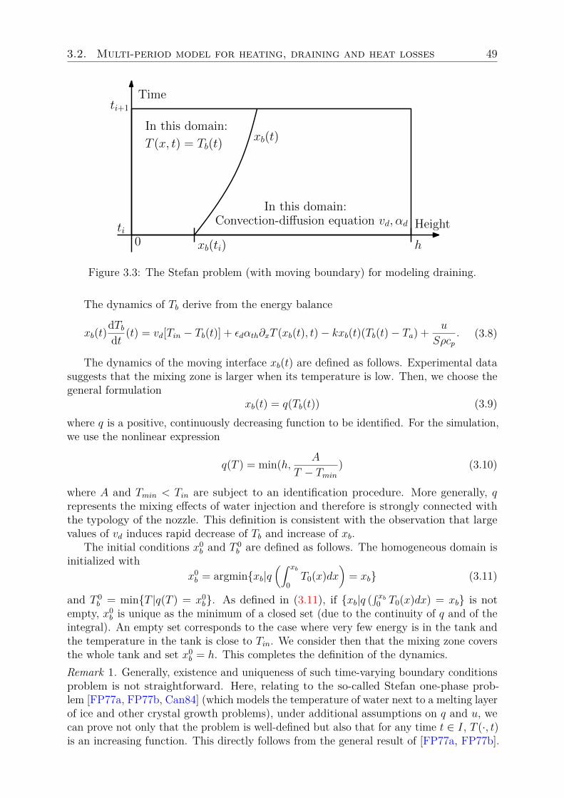
Figure 3.3: The Stefan problem (with moving boundary) for modeling draining.
The dynamics of the moving interface xb(t) are defined as follows. Experimental datasuggests that the mixing zone is larger when its temperature is low. Then, we choose thegeneral formulation
xb(t) = q(Tb(t)) (3.9)where q is a positive, continuously decreasing function to be identified. For the simulation,we use the nonlinear expression
q(T ) = min(h, A
T − Tmin) (3.10)
where A and Tmin < Tin are subject to an identification procedure. More generally, qrepresents the mixing effects of water injection and therefore is strongly connected withthe typology of the nozzle. This definition is consistent with the observation that largevalues of vd induces rapid decrease of Tb and increase of xb.
The initial conditions x0b and T 0
b are defined as follows. The homogeneous domain isinitialized with
x0b = argminxb|q
(∫ xb
0T0(x)dx
)= xb (3.11)
and T 0b = minT |q(T ) = x0
b. As defined in (3.11), if xb|q (∫ xb
0 T0(x)dx) = xb is notempty, x0
b is unique as the minimum of a closed set (due to the continuity of q and of theintegral). An empty set corresponds to the case where very few energy is in the tank andthe temperature in the tank is close to Tin. We consider then that the mixing zone coversthe whole tank and set x0
b = h. This completes the definition of the dynamics.Remark 1. Generally, existence and uniqueness of such time-varying boundary conditionsproblem is not straightforward. Here, relating to the so-called Stefan one-phase prob-lem [FP77a, FP77b, Can84] (which models the temperature of water next to a melting layerof ice and other crystal growth problems), under additional assumptions on q and u, wecan prove not only that the problem is well-defined but also that for any time t ∈ I, T (·, t)is an increasing function. This directly follows from the general result of [FP77a, FP77b].
50 Chapter 3. Multi-period dynamical modeling
0 20 40 60 80 100
20
30
40
50
60
70
80
H e ig h t (% o f m a x .)
Tem
perature(oC)
0 20 40 60 80 100
20
30
40
50
60
70
80
H e ig h t (% o f m a x .)
Tem
perature(oC)
(a.1) Plateau and backward flow (b.1) Plateau and backward flow
0 20 40 60 80 100
20
30
40
50
60
70
80
H e ig h t (% o f m a x .)
Tem
perature(oC)
0 20 40 60 80 100
20
30
40
50
60
70
80
H e ig h t (% o f m a x .)
Tem
perature(oC)
(a.2) Single thermocline (b.2) Single thermocline
0 20 40 60 80 100
20
30
40
50
60
70
80
H e ig h t (% o f m a x .)
Tem
perature(oC)
0 20 40 60 80 100
20
30
40
50
60
70
80
H e ig h t (% o f m a x .)
Tem
perature(oC)
(a.3) General scenario (b.3) General scenario
Figure 3.4: Comparisons of the physics-based model in § 2.1.4 (a) and the proposedmulti-period model (b), against experimental data (black), simulation are in blue.
Remark 2. If ∃t ∈ [0,∆t] s.t. xb(t) = h, the previously defined dynamics is halted and isreplaced for later times by
hdTbdt (t) = vd[Tin − Tb(t)]− kh(Tb(t)− Ta) + u
Sρcp
xb(t) = h
(3.12)
defining T (·, t) = Tb(t) over the whole tank.The description above defines the function FIII : given a constant draining vd and
heating u, FIII is the mapping from T0(·),∆ti, vd and u to the solution T (·, s) of (3.7),(3.8), (3.9) at time ti+1. In other words
FIII(T (·, ti),∆ti, u, vd) = T (·, ti+1).
3.3. Comparison against experimental data and physics-based model 51
Numerical considerations
As in § 3.2.2, this system can be solved numerically with finite difference schemes, jointlywith an ODE solver for the state Tb with the same time-step.
3.2.5 Summary of the multi-period modelThe definitions of functions FI , FII , FIII above allow an easy computation of the tem-perature profile at any final time tf : given a succession of phases separated by timesT = (t0, t1, ..., tm = tf) and an initial profile T (·, t0), intermediary profiles T (·, ti) arecomputed by successive applications of these functions, using the constant values of u andvd during each phase.Remark 3. Denote E ⊂ L∞(Ω) the set of increasing, piecewise continuous and continuouslypiecewise differentiable functions. Each of FI , FII , FIII maps the profiles from E to E,ensuring that our problem is well-defined.
3.3 Comparison against experimental data andphysics-based model
The multi-period model has been compared against experimental data under the sameconditions as in Chapter 2. Comparisons with previously obtained numerical results (usingthe model from § 2.1.4) show clear improvements both during draining periods (with thevanishing of the temperature and thermocline shifts) (see Fig. 3.4 (a.2)(b.2)) and duringheating periods (with an improved estimation of the plateau distribution and the backwardflow) (see Fig. 3.4 (a.1)(b.1)). The changes have a positive impact on the accuracy of themodel, as is reported in Table 3.1, in which the statistics of the absolute difference betweensimulation and experimental data has been used as a quality index (for the whole set ofdata): with the multi-period model, 96.8% of predicted temperatures have an error lowerthan 4 oC. Most importantly, a significant speedup is obtained. The low computationalcomplexity of the multi-period model enables its implementation in the envisioned “smartEHWT” applications.
Err. 0-2 oC 2-4 oC 4-6 oC 6-8 oC 8 oC+ TimePhysic-based model 53.9% 22.9% 10.7% 5.1% 7.4% 2435.6 sMulti-period model 82.3% 14.5% 2.0% 0.6% 0.6% 4.6 s
Table 3.1: Comparison of absolute difference between experimental value and modelprediction; computational time. Percentage of sample for each error interval.
3.4 SummaryIn this chapter, we have proposed a new model for an EHWT. This model is based onexperimental observations. It has the advantages of being accurate and computationallylight.
Thanks to these performance improvements, the multi-period model can be used toaddress the optimization problems P1, P2 considered in the thesis.
52 Chapter 3. Multi-period dynamical modeling
Very generally, in the context of “smart EHWT”, this model can be used to estimatethe temperature profile of the water contained in the tank, from an initial profile, heatingand draining histories. In practice, this requires a flow sensor (either at the input oroutput of the tank), and means for logging the power injected via the heating element.To estimate the initial condition, an internal temperature sensor can be used. In mostEHWT installed in the French market, such a sensor is already installed at the bottom ofthe tank in the thermostat. It is coupled with the heating element (see Fig. 1.1): heatinggoes on until this sensor detects a temperature of Tmax. The description of the thermostat,and the properties of the two models introduced earlier suggest that, when the sensedtemperature equals Tmax, the temperature of the water is uniformly equal to Tmax.
When coupled with the flow sensor, the thermostat sensor allows us to identify an open-loop model with occasional resetting of the profile. Starting with a uniform temperatureprofile Tmax, we compute the subsequent profiles using the model and the data of theinjected power and drained water. At each occurrence of Tmax measured by the sensor,we replace the profile by an uniform profile to ensure that the profile is calibrated on aregular basis. These can form the basis of a general state observer for this distributedparameter system.
Chapter 4
Autoregressive modeling fordomestic hot water consumption
Modèlisation autoregressive de la consommation d’eau chaude sanitaire. Dansce chapitre, nous étudions les propriété statistiques de la consommation d’eau chaudesanitaire au cours du temps. Sont étudiés : la distribution des amplitudes des soutirages,le comportement du consommateur sur une journée, et les durées entre deux soutiragessuccessifs. Un résultat marquant est que la durée entre deux soutirages successifs suit unedistribution de Weibull. Un modèle conditionnel autorégressif est proposé pour la suite deces durées, il est validé par des données expérimentales.
In this chapter we study one of the inputs of the previously introduced model: theconsumption of domestic hot water.
Users drain hot water from their EHWT at various times of the day. For comfort,delivery of hot water at all times is a constraint that must be satisfied at best. In advancedheating control strategies, a model of the user demand can be used, through the multi-period model developed in Chapter 3 to estimate, at any time, the state of charge of thetank as a function of heating and domestic hot water consumption. This states serves toevaluate (and guarantee) the availability of hot water for the user. In this chapter, weperform some investigations on the dynamics of domestic hot water (DHW) consumption,which has a random nature.
In the literature, many studies have focused on describing weekly or seasonal consump-tion patterns, or have presented hour-per-hour mean consumptions [VDS87, MT97, PPS95].At smaller times scales, the water drains appear as a sequence of quasi-instantaneousdrains (see Fig. 4.1). As can be observed on experimental data, the time of occurrenceof these drains is not fixed, but is stochastic. Some models representing drains as pointprocess have been developed. One such typical approach can be found in [JV00], in whichan approach based on aggregation of types of uses allows to generate minute-per-minuteload profiles, in [PG01], in which forecast over 2 days are generated using the Kalmanfilter, and in [HB10] which distribute clusters of drains following a hour-per-hour meanconsumption pattern. Nevertheless, more advanced stochastic modeling of the temporalcorrelation in the sequence, based on data analysis, would represent some valuable ways ofimprovement, especially in our context of heating strategy design. This chapter aims atestablishing such statistical properties. We develop an autoregressive model for domestic
54 Chapter 4. Model for hot water consumption
Min500 1000 1500 2000 2500
Dra
in(L
)
0
2
4
6
8
10
12
Drain
Figure 4.1: An example of sequence of drains for an household over 48 h. (experimentalresults)
hot water consumption.Domestic hot water consumption aggregates various uses in a household: baths, cleaning,
cooking, etc. The durations of resulting drains range from a few seconds to a few minutes.They can be represented as quasi-instantaneous events of various magnitudes in the scaleof the day. These drains can be described as a volume of hot water or a quantity of energytaken from the tank (the energy contained in hot water being defined with respect to acold water temperature reference). To model the drain sequence, one needs to describewhen the drain happens, and how much hot water is consumed during those drains (wemake the assumption that two drains occurring within a single minute correspond to asingle bigger drain). The following statistical properties are considered: i) the distributionof the magnitude of the drains, ii) a daily pattern of the start times of consumptions, iii)the time between two successive drains. This defines a stochastic process for the total hotwater consumption DHWC(t) at time t of the form
DHWC(t) =+∞∑j=1
Mjθ(t− tj) (4.1)
where tj andMj are the time of occurrence and the magnitude of the drain j, resp., and θ(t)is the Heaviside function: θ(t) = 0 if t < 0 and θ(t) = 1 if t ≥ 0. Classically, the magnitudeof the drains can be characterized through frequentist inference [Ney37], by estimating aprobability density function from the frequency of the data. Results obtained with thisapproach are presented in Section 4.1. The times of occurrence of the drains are morecomplex to describe. The consumption start times are related to the number of personsin the household and their domestic habits. As will be shown in Section 4.2, they are
4.1. Frequentist inference for the water drains distribution law 55
distributed according to an average daily pattern. Then, the time between two successivedrains follows a Weibull distribution. This is shown in Section 4.3. This observationallows to define a Weibull Autoregressive Conditional model for DHW consumption, whichis presented in Section 4.4. There, a validation is performed using data gathered in 11distinct households with EHWT equipped with flow meters and temperature sensors, overperiods ranging from 292 to 337 days, with a sampling time of one minute.
4.1 Frequentist inference for the water drains distri-bution law
A simple way to model the diversity of magnitude of the drains is to represent thedrains as random variables governed by the same probability law. Since the drains arepositive, this probability law can be represented with a probability density functionon [0,+∞[ (see Fig. 4.2). The probability distribution reported in Fig. 4.2 has beenestimated with a frequentist approach, for all households and all measurements. Thedisplayed distribution law is the frequency of occurrence of each drain for a large numberof measurements. An interesting observation is that four distinct peaks are visible inthe filtered distribution function. This is in accordance with the results presented in[JV00], obtained by considering four types of uses (small and medium drains, shower bathand bath tub). If needed, these results could be refined by taking into account that themeasurements are strongly related to the habits of the households (e.g. baths), the time ofthe day and the season. For households equipped with additional sensors, the conditionaldistribution could be estimated online. However, we do not consider this refinement here.
4.2 Daily pattern for the start times of drainsThe hot water consumption is strongly related to the habits of the house occupants. Also,it is clearly visible in the data (as could be expected) that the drains mostly take place atcertain times of the day (see Fig. 4.1). In fact, a daily pattern can be defined. For this,one can simply consider the mean value of the number of drains at a given time of theday, for each household. The procedure is as follows. This procedure is commonly used instatistics (e.g. to determine the intensity function of a non-homogeneous Poisson process[Ruw07]). Given a household, we represent each of its n set of 24 h measurements (labeledby k = 1...n) with a function Nk(t) that represents the number of drains having occurredin this day over the interval [0, t], for t ∈ [0, 24h]. In other words, consider any day k andthe sorted drain times tk1, ..., tkm, then Nk(t) is defined as
Nk(t) =m∑j=1
θ(t− tkj ). (4.2)
Then, we define the daily pattern as the mean of these functions
M(t) = 1n
n∑k=1
Nk(t). (4.3)
This function, defined over the time interval [0, 24h], gives, for any household, theaverage (expected) number of drains that should have occurred at time t (see Fig. 4.3): itis representative of the habits of this household in terms of frequency of the drain. The
56 Chapter 4. Model for hot water consumption
Water drain (L)0 2 4 6 8 10 12 14 16 18 20
Nor
mal
ized
distr
ibution
0
0.002
0.004
0.006
0.008
0.01
0.012
0.014
0.016
Experimental distributionSmoothed experimental distribution
Figure 4.2: Experimental probability distribution of drain magnitudes (over the wholerecorded sequences). The smoothed plot highlights 4 distinct peaks. (experimental results)
function (4.3) obtained with the discussed dataset is reported in Fig. 4.3. The presenceof sharp transients between low slope regions shows that the average function (4.2) isrepresentative of the individual behaviors in each household. High slopes correspond toperiods with frequent drains.
4.3 Distribution of the time between two successivedrains
The time between two successive drains yki = tki − tki−1 (during a day k) is also related tothe habits of the house occupants. Therefore, we isolate data accordingly. In the casewhen the number of drains over time Nk(t) are samples of a non-homogeneous Poissonprocess (i.e. the drains are not correlated), it is possible to construct adjusted incrementswith the mean value function M(t), that must follow an exponential distribution. As willappear, this assumption is not valid in our case, but we still perform the same analysis,yielding different conclusions. The construction is done the following way. For each periodk of 24 h, a set is constructed by taking the image of each drain time tk1, ..., tkm, throughthe function M (see Fig. 4.4). The M(tki ) are then used to define the set of successiveincrements
υki = M(tki )−M(tki−1).These variables have an interpretation: for any day k, υki is the average increment of
the number of drains from tki−1 to tki . Its expected value (for all possible k) is 1. These
4.3. Distribution of the time between two successive drains 57
Min200 400 600 800 1000 1200 1400
Mea
nnum
ber
ofdra
ins
0
2
4
6
8
10
12
14
16
18
Experimental daily pattern
(a) Weekday
Min0 500 1000 1500
Mea
nnum
ber
ofdra
ins
0
2
4
6
8
10
12
14
16
Experimental daily pattern
(b) Weekend
Figure 4.3: Two examples of averaged daily cumulative number of drains. Experimentalresults are in blue, and and smoothed version is in orange.
58 Chapter 4. Model for hot water consumption
time
24ht1 tmti
υi
Daily pattern cumulative function M(t)
yi
Figure 4.4: Construction of the adjusted increments.
normalized increments (represented in the ordinate axis in Fig. 4.4) are assumed to beindependent from the choice of the households. They are representative of the correlationbetween successive drains. The υki are distributed in the [0,+∞[ interval. Using the wholedataset, an experimental cumulative distribution function (CDF) can be obtained. It isreported in Fig. 4.5. Remarkably, this function shows a good fit to h(υ) = 1− exp(υδ/κ),which corresponds to the CDF of the Weibull distribution of shape parameter δ andscale parameter κ [MXJ04]. Among other possibilities (exponential distribution, Gammadistribution, Beta distribution), this is (by far) the best fit. In the literature, the Weibulldistribution is commonly used to model failure rates over time, the parameter δ definingthe nature of the process. The case δ = 1 corresponds to an exponential distribution. Ifδ < 1, then the occurrence of an event raises the probability of a closely following event(cases of immediately consecutive events are frequent). On the contrary, the case δ > 1corresponds to the case when successive events are spaced out.
To establish that the experimental data follow the assumed distribution, a graphicalmethod can be employed. The probability plot consists in plotting two CDF, one againstthe other: if the two distributions are similar, the points of the probability plot shouldlie on a straight line. Further, for the Weibull distribution, the shape parameter δ cansimply be deduced from the slope [MXJ04]. Such a plot is reported in Fig. 4.6, wherethe distribution of the experimental adjusted increment set is plotted in logarithmic scaleagainst a generated data set following a normalized Weibull distribution. The apparition ofa straight line in the plot suggests that the Weibull model is relevant. Typically, δ = 0.53.However, the linearity is not perfect for small increments, and a jerky character of theline can be observed for small increments. A reduction of the sampling time can increasethe accuracy (here the one minute sampling time is in conflict with the very shorts timeintervals separating two successive drains).
4.3. Distribution of the time between two successive drains 59
Normalized increments0 5 10 15
Cum
ula
tive
Den
sity
Funct
ion
0
0.1
0.2
0.3
0.4
0.5
0.6
0.7
0.8
0.9
1
Experimental CDFWeibull CDFExponential CDF
Figure 4.5: Experimental CDF for the adjusted increments compared to the Weibull andexponential CDF.
Data10-3 10-2 10-1 100 101 102
Pro
bab
ility
0.0005
0.001
0.005
0.01
0.05
0.1
0.25
0.5
0.75 0.9
0.99 0.999 0.9999
Probability plot for Weibull distribution
Figure 4.6: Probability plot of the data against the Weibull distribution.
60 Chapter 4. Model for hot water consumption
4.4 An autoregressive model for domestic hot waterconsumption
Given the studies above, we incorporate the Weibull distribution in a point processmodel for the drains. In the literature, the Weibull distribution is often associated withAutoregressive Conditional Duration (ACD) models [Cro13], initially developed by Engleand Russels [ER98]1.
ACD models are based on an autoregressive structure for the conditional duration oftime lapses between two events [ER98]. The idea is to generate a sequence of n durationswith an autoregressive law depending of preceding duration. The duration number i, seenas a stochastic variable υi, is given by the mean equation
υi = ψiεi,
in which the εi are independent and identically distributed following a given probabilitylaw, with mean value equal to 1, and
ψi = E[υi|Fi−1]
is the mean duration conditionally to the information available after the last eventrepresented by the filtration Fi−1. A filtration is an increasing (in the set theory sense)sequence of σ-fields. It is used to represent the (increasing) information available at a eachstep. Here, the Fi is the natural filtration generated by the sequence of the εi. For moreinformation on filtration, see e.g. [RW00].
The linear ACD(1, 1) model is given by the equation
ψi = ω0 + ω1υi−1 + ω2ψi−1
for ω0 > 0, ω1, ω2 ≥ 0.Several distribution can be given to the εi. The most classical are the Exponential ACD
(EACD) and Weibull ACD (WACD). ACD(p, q) models can be defined by extending theautoregressive character to order p for the υi and q for the ψi, but we will limit ourselvesto the case (p, q) = (1, 1). For a given household, identification of parameters ω0, ω1, ω2and shape parameter δ of the Weibull distribution is needed. For this problem, we usethe off-the-shelf Estimation and Simulation of ACD models Matlab code produced by M.Perlin (see [Per12]).
Then, the identification procedure to model drain occurrence for a given household isthe following.
1. Gather historical data on the occurrence time of the drains in the the household.
2. Using this data, compute the daily pattern M(t) and the distribution law of themagnitude of the drains as described in Section 4.1 and Section 4.2 .
3. Using the occurrence time and the daily pattern, construct the set of increments υi.
4. Identify parameters ω0, ω1, ω2 and δ (for instance with the software package [Per12]).1It was initially used to model seismic aftershocks and to forecast the distribution of a succession of
duration times between two transactions in stock market [Tsa07]
4.5. Summary 61
This procedure permits to represent each household with model parameters
M(·), ω0, ω1, ω2, δ.
The WACD parameters are used to generate sets of increments υi, which are then used toconstruct time of occurrence of drains using the relation
ti = M−1(υi +M(ti−1)).
Finally, the magnitude of the drain can be drawn from the distribution law previouslydefined.
Model validationTo validate the model, we apply the identification procedure for each households ofthe dataset described earlier. Then, the obtained parameters are used to generate setsof increments. Finally, both experimental and simulated increments are compared ina probability plot in Fig. 4.7. The results are satisfactory, at the exception of longexperimental durations that are not well represented in the model. A possible explanationis that those duration may correspond to vacation periods (holidays), and represent outliersthat we could not isolate from the dataset. This stresses the necessity to add an overlayto account for exceptional events in future studies. As a mean of comparison, probabilityplot against duration stemming from uniform distribution of drains on a 24 h period, andagainst an EACD model are depicted in Fig. 4.8 and Fig. 4.9. The conclusion of thisanalysis is that the Weibull distribution is, by far, the best standard distribution for anACD model at the light of the data under consideration.
4.5 SummaryIn this chapter, an autoregressive time series model for DWC consumption has beendeveloped. Interestingly, the model stresses that if the user is draining water, then heis very likely to drain more water shortly. Consequently, an online computing of theconditional mean duration ψi gives a representative index of the drain general trend. Asmall value indicates a general increase of consumption, and piloting strategies can beupdated online to take into account the high probability of future drains. Very generally,this model can be used for “smart EHWT” piloting applications. Indeed, it can be usedto generate realistic scenarios of consumption, subsequently used to test the robustness ofpiloting strategies. At large scales, for a large number of EHWT, stochastic modelling ofthe consumption can be generalized into models for the distribution of the state of chargeof the tanks, using e.g. Fokker-Planck equations. This will be shown in Chapter 8.
62 Chapter 4. Model for hot water consumption
Data0 2 4 6 8 10 12 14 16
Sim
ula
tion
0
2
4
6
8
10
12
14
16
Figure 4.7: Probability plot of the WACD simulation increments against experimentalincrements, for the whole set of data. (our proposed model)
Data0 5 10 15
Sim
ula
tion
0
10
20
30
40
50
60
Figure 4.8: Probability plot of the simulation increments when the uniform distribution isused, against experimental increments, for the whole set of data. (alternative model)
4.5. Summary 63
Data0 5 10 15 20 25 30 35 40
Sim
ula
tion
0
10
20
30
40
50
60
Figure 4.9: Probability plot of the EACD simulation increments against experimentalincrements, for the whole set of data. (alternative model)
Chapter 5
Input-output representation ofEHWT
Représentation entrée-sortie d’un CEJ. Dans ce chapitre, on propose une représen-tation entrée-sortie d’un CEJ. Elle repose notamment sur la définition de trois variablesd’intérêt : l’énergie disponible dans le ballon, l’énergie de délai et l’énergie non disponible,chacune Ãľtant définie grâce au profil de température dans le ballon. Ces définitionspermettent de représenter l’état du ballon avec trois variables, et ouvrent la voie à laconception d’un “CEJ connecté”.
To design control and optimization advanced strategies, we define key indicatorsrepresenting the state of each EHWT. By proceeding this way, we reduce a distributedstate (the temperature profile in the tank) into a finite number of well-chosen variablesdirectly useable to evaluate comfort constraints. A focus is put on the supply of waterto consumers when piloting the heating of the tank. Considering that the temperatureprofile defined above is increasing with height because of stratification (see Chapter 2and 3), further simplifications are possible. One can define two variables representing theenergy contained in the water of temperature above a comfort temperature set by theuser (i.e. an energy which can be used for consumption), and a energy that representsthe functioning delay of EHWT for hot water production. The delay energy representsthe energy necessary for the plateau introduced earlier to reach the comfort temperature.Once this level is reached (after the so-called “delay”), further heating raises the energyavailable for consumption. A third variable of interest is used to represent the energy inthe tank unavailable for consumption, i.e. contained in water heated below the comforttemperature.
This triplet of variables offers a simple representation of an EHWT. Interestingly,the complex variation of the temperature profile is well represented by the dynamics ofthis low-dimensional state. This representation is an intermediate solution between thedistributed parameter models developed earlier in the thesis and single integrator modelscommonly found in the literature. It models the complex dynamics of the comfort variablesand the lag observed in the production of hot water, in a simple yet non-simplistic manner.
66 Chapter 5. Input-output representation of EHWT
Temperature
h
Tcom
Tin
aτ
µ
Tmax
ycFigure 5.1: Temperature profile inside an EHWT after a drain. Available, delay andreserve energies correspond to area defined by the profile.
5.1 Definition of user comfortFollowing the description above, the temperature T of the tank is a continuously increasingfunction of height. We assume that the water injected in the tank is at constant temperatureTin, which constitutes a lower bound of the temperature profile, and that the heatingprocess is driven by turbulence generated by buoyancy effects during the heating process,which is the cause of a local mixing in the bottom of the tank. We consider that this mixingis perfect on the plateau, and does not affect the temperature profile in the upper partof the tank. During the process, the plateau grows and gradually covers the whole tank.Thanks to a thermostat, the user specifies a temperature Tmax at which the heating has tobe stopped to prevent overheating. As a result of the heating process, if the temperatureat the bottom of the tank is Tmax, then the temperature in the tank is uniformly at Tmax.The user also specifies a comfort temperature Tcom. Water having temperature higher thanTcom can be blended with cold water to reach Tcom and is therefore useful, while waterhaving temperature lower than Tcom is useless.
5.2 Definition of variables of interest: available, delayand reserve energies
We simplify the system using the 3 following state variables, depicted in Fig. 5.1,The available energy a is defined as the energy contained in the zones having temperature
greater than the comfort temperature Tcom. This constitutes a direct comfort index for theuser. The situation when a reaches the value 0 and a water drain is applied correspondsto the fact that the consumer is trying to consume hot water when none is available, and
5.3. Summary: towards the “smart EHWT” 67
therefore that the comfort constraints are broken.The delay energy τ is defined as the energy required by the plateau to reach the
temperature Tcom. If the tank is heated at constant maximum power, and withoutaccounting for drains and heat losses, τ is proportional to the time necessary to reach astate in which a can effectively be increased by the heating process.
The reserve energy µ is defined as the energy contained in the tank that is currentlyunavailable for consumption, i.e. the energy contained in the water under Tcom. When,during the heating process, τ reaches the value 0, the energy µ becomes available toconsumption: this generates an immediate (discontinuous) increase of a, and µ is resetto 0.
The rationale behind these definitions is that to plan the heating, we account for thetime left before the energy reserve embodied by a (in the total energy a+ µ) is consumed,and the time necessary to provide new hot water, embodied by τ .
Fig. 5.2 reports examples of the dynamics of these variables. A drain (shown in Fig. 5.2(a) and (e)(f)) is mainly characterized by a decrease of a and an increase of τ , with a slightraise of µ due to an energy transfer from a. On the other hand, in the heating reportedin Fig. 5.2(b)(c)(d), τ decreases at the same rate as µ rises, and after a gap at τ = 0characterized by an energy transfer from µ to a, a progressively increases.
Given T (·) the (non necessarily strictly) increasing temperature profile of the waterdefined on [0, h], the above definitions yield the following expressions of a, τ , µ as
a = Sρcp
∫ h
yc
T (y)dy
τ = Sρcp
∫ yc
0(Tcom − T (y))dy
µ = Sρcp
∫ yc
0T (y)dy
where ρ and cp are the density and the heat capacity of water, respectively, and yc isdefined as
yc , miny|T (y) = Tcom.In the sequence, we will use the notation
z , (a, τ, µ).
The triplet z is a low-dimensional representation of the tank. This representationcomes at the cost of a loss of information in comparison to a distributed profile. However,due to the increasing nature of the profile and the fact that the thermocline is often steep,the triplet gives a satisfactory schematic view of the distributed profile (see Fig. 5.3).Moreover, it captures well the information necessary to design control strategies.
An example of the variation of z over a 24 h run with given drains and heating ispresented in Fig. 5.4. In this figure, the variations of the three variables are computed withexperimental data (in blue) and compared with simulation with the multi-period model(in red) and a simple single-zone model (in black). The figure highlights the accuracy ofthe multi-period model that is able to kindly reproduce the evolution of z.
5.3 Summary: towards the “smart EHWT”The definition of the variable of interest concludes the modeling efforts conducted so far. Atthis stage we can now formulate an input-output representation of the EHWT, presented
68 Chapter 5. Input-output representation of EHWT
Temperature
h
Tcom
Tin
aτ
µ
Tmax
yc
Temperature
h
Tcom
Tin
a
τ
µ
Tmax
yc(a) After a drain (b) During the heating process
Temperature
h
Tin
a
Tmax
Tcom
Temperature
h
Tin
a
Tmax
Tcom
(c) After the gap (d) Uniformly hot tankTemperature
h
Tcom
Tin
aτ
µ
Tmax
yc
Temperature
h
Tcom
Tin
τ
µ
Tmax
(e) After a drain (f) Large drain
Figure 5.2: Schematic variation of the state z during heating and draining.
in Fig. 1.4. These works allows to design the architecture of a “smart EHWT” equippedwith a chip set as depicted in Fig. 5.5.
In such tanks, histories of electricity consumption and water drains allow to compute,thanks to the multi-period model, the distributed temperature profile of the water inthe tank. Variables of interest derived from the profile are transmitted to an externaldecision center, which, in return, transmits a heating strategy back to the “smart EHWT”.
5.3. Summary: towards the “smart EHWT” 69
Temperature
h
Tcom
Tin
aτ
µ
Tmax
yc
schematic profile
Figure 5.3: Available, delay and reserve energies and schematic reconstruction of theoriginal temperature profile.
If necessary, this strategy can even be test-proven by the “smart EHWT” itself, using thedomestic hot water consumption model and the multi-period model numerically treatedby the onboard chipset. Eventually, the strategy can be applied in real-time (up tocommunication and computation lags).Remark 4. Alternative architectures are possible. For instance, an intermediate decisioncenter can also be integrated to the chipset to generate heating strategies for the EHWTwith respect to a price signal.
If such smart tanks are to be developed and deployed, their use in coordinated strategieshave to be designed to solve P1 and P2. The second part of this thesis focus on suchproblems.
70 Chapter 5. Input-output representation of EHWT
2 4 6 8 10 12 14 16 18 20 220
200
400
Draining (l/h)
2 4 6 8 10 12 14 16 18 20 220
500
1000
Heating power (W)
2 4 6 8 10 12 14 16 18 20 22
#107
0
5
Available energy (J)
2 4 6 8 10 12 14 16 18 20 22
#106
0
10
Delay energy (J)
Time (h)2 4 6 8 10 12 14 16 18 20 22
#107
0
2
4Reserve energy (J)
Figure 5.4: Variation of z = (a, τ, µ) over a 24 h run. a: available energy, τ : delay energy,µ: reserve energy. Blue: experimental data. Red: simulation using the multi-period model.Black: Simulation using a single-zone model (with reconstructed variables).
5.3. Summary: towards the “smart EHWT” 71
Multi-periodmodel
DHWC model
Chipset
Power control
uz
Flowmeter
OutputT
Figure 5.5: Schematic view of the “smart EHWT”.
Part II
Control of groups of EHWT
Chapter 6
Small-scale groups: discrete-timeoptimization
Optimisation discrete pour un parc de petite taille. Dans ce chapitre, nousproposons un modèle discret d’évolution de l’état du ballon représenté par les troisvariables d’intérêt définies précédemment. Ce modèle permet de formuler un problèmed’optimisation du fonctionnement du ballon sous contraintes de confort. Ce problèmepeut lui-même se ré-écrire comme un programme linéaire en nombre entiers, de telle sorteque la résolution est réalisable avec des logiciels standards. Des résultats numériques sontprésentés et comparés avec la stratégie historique d’heures pleines/heures creuses.
In this chapter, we propose an optimal heating strategy for a first use-case focused ona small group of “smart EHWT” (from 1 to 4, typically). Using the variables of interestintroduced in Chapter 5, we set up a discrete-time model for the dynamics of the triplet,as well as an optimization framework to solve problems P1 and P2. This frameworktakes the form of a mixed integer linear program (MILP) for problem P1, or a mixedinteger quadratic program (MIQP) for problem P2. In the case of P1, the computationof the optimal solution is light and may be directly embedded in the chipset of a “smartEHWT”(which could embed mildly powerful processor such as ARM Cortex-A7 MPCore).
The chapter is organized as follows. Section 6.1 is dedicated to the discrete-time model.The dynamics serve to formulate P1 and P2 in discrete time. Section 6.2 shows howto recast such problems as mixed integer linear/quadratic programs, which yields easynumerical solution. Numerical results are presented in Section 6.3.
6.1 Discrete-time dynamics and optimization prob-lems
6.1.1 Discretization and notationsFor a given tank, we consider the variation of z = (a, τ, µ) over a finite time horizonthat we discretize into uniform time-steps [0, ..., n]. We note (a0, ..., an), (τ0, ...τn) and(µ0, ..., µn) the values of a, τ , µ at each of these time-steps.
At each time t ∈ [0, ..., n− 1], energy is consumed by the user (through draining) by anamount dt that we consider as known. Energy is introduced via the heating element by an
76 Chapter 6. Small-scale groups
amount ut ∈ [0, umax]. We divide the later into two parts vt and wt, representing the shareintroduced in at and in µt, respectively. Finally, we define the variable φt which representsa flow of energy from µt to at+1, taking place in conditions that will be described below.
6.1.2 Dynamics and constraintsBalance equations
For any index t, the dynamics of zt is given by the energy balances
The various phenomena described earlier appear in the righthand side of these equations.Heat losses, modeled with an exponential decay, are characterized by the decrease of aand µ at a rate p, the energy from the later contributing to a raise of τ (see Fig. 5.1).The energy consumed by the user during one time step is split between a and µ with aratio α, 1− α and affects τ with a coefficient β.
Definition of the heat source terms vt, wt
As has been seen before, the energy is injected at the bottom of the tank via the heatingelement. As a consequence, the heating has no impact on the available energy a when τ > 0,but, instead, tends to reduce τ and increase µ. When the value of τ is 0, the injectedenergy becomes immediately available. This can be modeled by dividing ut into twoshares vt and wt representing, respectively, the part of the injected energy going into aand µ, and subject to the following conditions
Given the balance equations (Dt)-(Ft), if τt+1 > 0 then no energy can be introducedin at+1 (i.e. vt = 0 and wt = ut) and, if τt+1 = 0 the value of wt has to compensate forheat losses pµt and/or energy drain from the user βdt, while the remainder is introducedin at+1.
Definition of internal energy flow φt
The flow φ is always equal to 0, except when τ reaches the value 0. Then, the valueof φ is defined by the fact that all the energy µ suddenly becomes available. This can bedescribed as follows
0 = φtτt+1 (Gt)0 ≤ φt (Ht)
τt+1 = 0⇒ µt+1 = 0. (It)
Remark 5. Given a state zt, a drain dt and a heat injection ut, relations (At)-(It) uniquelydefine vt, wt, φt and therefore the future state zt+1 (under the assumption that τt+1 has tobe nonnegative).
6.1. Discrete-time dynamics and optimization problems 77
Bounds and comfort constraints
Here, we determine some constraints zt is subject to for all t. This defines the admissiblecontrols that allow each zt to respect these constraints.
By definition, the delay energy is positive. We impose τt ≥ 0 for all t, in order toimpose a heat injection with vt if τ reaches 0.
Define emax = Sρcp(Tmax− Tin) the maximal energy that can be contained in the tank,and
λ ,Tcom − TinTmax − Tin
. (6.1)
To ensure that no energy is drained more that the tank can provide, we require at ≥ 0and µt ≥ 0 for all t, and that the tank is not overheated, we require at ≤ emax, τt ≤ λemax,and µt ≤ λemax for all t.
Finally, physical constraints on the total energy imply
λat + τt + µt ≤ λemax
λemax ≤ at + τt + µt. (6.2)
Given these relations, we define the following domain
For any given (a0, τ0, µ0) ∈ Ω and d = (d0, ..., dn−1) ∈ Rn+, and for any chosen con-
trol sequence u = (u0, ..., un−1) the relations (At)-(It) for t ∈ [0, ..., n − 1] uniquelydefine (a, τ, µ, v, w, φ)t for all subsequent t. This allows us to define the admissible set U :
U(a0, τ0, µ0, d) = u ∈ Rn|the a, τ, µ, v, w, φ implicitly defined by (At)-(It)t∈[0,...,n−1]
satisfy (Jt) ∀t ∈ [0, ..., n].
In a practical sense, given initial conditions and a drain sequence, it constitutes the set ofheating sequences that do not break the comfort constraints of the user.
6.1.3 Objective function and formulation of the optimizationproblem
We consider that a0, τ0, µ0 and d are given and that a flat discrete-time price signal forelectricity over time (c0, ..., cn−1) is known. The optimization problem P1 can be written(for each tank) as
minu∈U(a0,τ0,µ0,d)
n−1∑t=0
ctut. (6.3)
This problem is therefore to search, for an EHWT, the heating strategy that minimizesthe cost of heating while ensuring a required supply of hot water to the user.
78 Chapter 6. Small-scale groups
τ
µ
λemax
forbidden line
τ
µ
λemax
Mτ = µ
enlarged forbidden area
λemax
λemax
Figure 6.1: Strengthening of (It).
In cases when several tanks can simultaneously be controlled with controls u1, ..., uk,and one can introduce the discrete-time objective for aggregated consumption (Pt)t∈[0,...,n−1].Then, the optimization problem P2 takes the form
min(u1,...,uk)∈U(a1
0,τ10 ,µ
10,d
1)×...×U(ak0 ,τ
k0 ,µ
k0 ,d
1)
n−1∑t=0
(Pt −k∑j=1
ujt)2. (6.4)
6.2 Mixed integer representation of the constraintsand dynamics
With the exception of the two product conditions (Et) and (Gt), and the condition (It), therelations (At)-(Jt) are linear equalities and inequalities in the variables (ut, at, τt, µt, vt, wt, φt)and therefore define a polytope of R7n, for each tank. Thus, we adapt (Et), (Gt) and (It)to give to problems (6.3) and (6.4) the structure of a linear and a quadratic program,respectively, that can efficiently be solved with commercial software (see e.g. [Gur15] or[IBM09]).
Strengthening of (It)
Given the setA = (τ, µ) ∈ [0, λemax]2|τ = 0⇒ µ = 0,
then, equivalently,
A = [0, λemax]2\(τ, µ) ∈ [0, λm]2|τ = 0, µ > 0.
A possible strengthening is
(τ, µ) ∈ [0, λemax]2|Mτt ≥ µt ⊂ A
where M > 0 (see Fig. 6.1). Instead of considering (It) we (conservatively) consider (I ′t)which has the linear form
Mτt ≥ µt, (I ′t)
6.3. Simulation results 79
chosing M > 0. This new relation has the linear form required in linear programmingformulations, and if emax is sufficiently large, only a small feasible regime (see Fig. 6.1) isleft out of the optimization problem.
Given this new relation, we define the polytope
Y(a0, τ0, µ0, d) = Y = (u, a, τ, µ, v, w, φ) ∈ R7n|(At)-(Dt), (Ft), (Ht), (I ′t) ∀t ∈ [0, ..., n− 1]
and (Jt) ∀t ∈ [0, ..., n] are satisfied.
Reformulation of (Et) and (Gt)
The product conditions (Et) and (Gt) correspond to 2n couples (vt, τt+1) and (vt, φt)consisting of two elements that cannot simultaneously be positive. These constraints havethe form of complementarity conditions (see [CD68]). In practical terms, each of thesecases can be encoded with binary or integer constraints and problems (6.3) and (6.4)written as a collection of linear programs (LP), respectively quadratic programs (QP),taking the form of a mixed-inter linear program (MILP) and a mixed integer quadraticprogram (MIQP).
A more careful look at the situation reveals that these kinds of sets are in fact frequentlyencountered in discrete optimization under the name of Special Ordered Set (SOS), andare associated with branch and bound strategies (see [BT70]). This considerably easesthe resolution for instances having reasonable dimensions. These strategies are oftenimplemented in linear programming solvers, see [Zus11].
As a result of the reformulation of (Et) and (Gt), and the strengthening of (It), we canpropose the following solution method.
Solution method
Given initial conditions (a0, τ0, µ0) and the drain sequence d, one can now solve by anyappropriate numerical method (e.g. branching strategies) the collection of LP/QP
minY ∈Y(a0,τ0,µ0,d)
n−1∑t=0
ctut (6.5)
ormin
Y 1,...,Y k∈Y(a0,τ0,µ0,d)
n−1∑t=0
(Pt −k∑j=1
ujt)2. (6.6)
indexed by the 2nk SOS on τ and µ.
6.3 Simulation results
6.3.1 Identification of the parametersIn the previously defined problems, values for most of the parameters are easy to deter-mine: Tcom, Tin, Tmax and therefore λ are either chosen by the user, or directly measuredfrom the water distribution network. On the other hand, the values of emax, p and umaxdepend on the type of EHWT. These data are provided by the manufacturer, and arereported in Table 2.1.
80 Chapter 6. Small-scale groups
The main difficulty is to determine the coefficients (α, β) of our model. They representthe effects of the energy drains (d0, ..., dn−1) on z.
In theory, the values of these two parameters depend on x, which breaks the linearity.In practice, their variations are small, except in some parts of the domain Ω, where thetemperature in a is close to Tcom (close to the border a + τ + µ = λm). Therefore, tokeep the linearity of the constraints, we assume that the two parameters are constant. Toreduce the cost of this assumption in terms of accuracy, we replace the constraint (6.2)with a+τ +µ ≥ λemax+ep, with ep appropriately chosen (for instance ep = 1
10emax). Usingthe model presented in Chapter 3 for identification purposes, we set the values α ' 1.2and β ' 0.4.
6.3.2 Simulations resultsTo test the relevance of our predictions, simulations with realistic parameters have beenconducted on simple cases that can readily be interpreted. The parameters correspondto the tank used for experimentation. The computations have been performed using theSCIP solver (see [Zus11]).
Several cases have been considered. We now detail the obtained results.
Two prices signal
In Fig. 6.2, we report the values of the control and the associated available water forproblem (6.5) with those prices. The optimization has been performed over a 48 h horizonwith 20min time step for a 24 h application of the control signal, to avoid side effects. Theresults show a reasonably smooth control signal, which heats the tank at the end of lowprices period, to limit consumption at high prices and reduce heat losses. This strategy ismore efficient than the heating at the beginning of the off-peak period, usually set up inpractice (the so-called night time switch). For this typical case, the gain for the consumeris of 13.2%, due to a heating strategy that limits heat loss while heating at the end oflow-price periods, and avoids overheating of the tank.
Spot prices
In Fig. 6.3, we report the values of the control and the associated amount of availablewater for problem (6.6) with the spot prices in Europe for a typical winter day, taken fromthe EPEX Spot Market (see [EPE14]). Again, the results show a sensible control, whichheats the tank at the end of low prices period, to limit consumption at high prices andreduce heat losses. The gain for the producer, in this case, is of 36.1% compared to thenight time switch strategy.
Peak shaving for several tanks
As an extension, we can also solve a problem of practical interest. We have run simulationson a set of several tanks with various initial conditions, with a problem defined as weightedsum of the criteria of problem (6.5) and problem (6.6): each tank is optimized against aprice signal, individually, and a global consumption is favored in the middle of the day inthe form of an additional load curve objective in the [10h, 13h] time window that may,for instance, answer to an upward adjustment request. The results of these simulationsare reported in Fig. 6.4, where each tank is represented with a different color.
6.3. Simulation results 81
0 5 10 15 200
0.5
1
Heating u (red), in % of max power, and normalized prices c (black)
0 5 10 15 200
0.1
0.2
0.3
0.4Drain d, in % of tank capacity
0 5 10 15 200
0.5
1Energies a (green), τ (blue), µ (black), in % of tank capacity
Figure 6.2: Optimization for a two price scenario.
82 Chapter 6. Small-scale groups
0 5 10 15 200
0.5
1
Heating u (red), in % of max power, and normalized prices c (black)
0 5 10 15 200
0.1
0.2
0.3
0.4Drain d, in % of tank capacity
0 5 10 15 200
0.5
1Energies a (green), τ (blue), µ (black), in % of tank capacity
Figure 6.3: Optimization for a spot prices scenario.
6.3. Simulation results 83
0 5 10 15 200
0.5
1
Normalized prices c (black) and peak requirements γ (cyan)
0 5 10 15 200
0.5
1
Heating u, in % of max power
0 5 10 15 200
0.5
1Energy a, in % of tank capacity
Figure 6.4: Simultaneous optimization of four tanks.
84 Chapter 6. Small-scale groups
6.4 SummaryThis chapter has proposed numerical methods to address the optimization problem P1 andP2 at stake in the thesis. The method is capable of handling a single or a small groupof EHWT. For this a simple dynamics for the 3 states representation of the EHWT, anda framework to optimally heat it with off-the-shelf solvers has been derived. We haveprocessed the optimization problems in deterministic cases, under perfect knowledge ofconsumptions over the optimization horizons. Practical online computation of heatingstrategies should account for the inherent stochasticity of users consumptions. Thedefinition of a set of realistic scenarios of drains for a given household using the modelpresented in Chapter 4 allows one to define a worst-case heating strategy. Stochasticprogramming also appear as promising solution but has not been explored.
If necessary, some sort of closed-loop feedback model predictive control could beemployed. Typically, in the envisioned “smart EHWT”, heating strategy could be computedon a 48 h horizon, with 15 min closed-loop intervals.
The method scales reasonably up to a number of 4 tanks. Typical computational loadsare reported in Table 6.1. Generalization to arbitrary numbers of tanks does not seemfeasible, as-is. The computational cost seems to increase exponentially with the numberof tanks. Thus, a global piloting using a single centralized optimization program does
Number of tanks Computational time (s)1 2.02 9.43 754.24 4756.4
Table 6.1: Computational times.
not appear as a viable solution. However, the tanks having separable constraints, theoptimization problem under consideration is compliant with decomposition-coordinationtechniques. In particular, the so-called price coordination (see [MMT71]) seems to applywell to the formulations considered in this chapter.
Chapter 7
Medium-scale groups: optimizationalgorithm for load-shifting
Algorithme d’optimisation du décalage de charge pour les parc de taille in-termédiaire. Dans ce chapitre, nous proposons la formulation du problème P2 dans lecas ou les périodes de chauffe restent indivisées, tout en prenant en compte l’effet despertes thermiques. Dans un second temps, une heuristique pour ce problème est proposée.Cette heuristique est testée sur huit instances représentatives des problèmes rencontrés enpratique.
In this chapter, we focus on a medium-sized groups of EHWT (from a few hundreds toseveral millions), each being characterized by its electric power and heat losses coefficient.We assume that they are remotely controllable.
As described in the introduction of the thesis, a consequence of the night time switch us-ing wired remote control of the group of EHWT in France is an overall decrease of theconsumption in the middle of the night when the electricity production costs are low. Thisis a detrimental effect for the electricity producer.
Instead of finely piloting each tank, we consider a rescheduling of each EHWT heatingin the night time, while keeping the heating period undivided, to attain a desired loadcurve for the whole set of EHWT, while ensuring individual users comfort. The idea is tominimize the malicious impact of complex dynamic effects taking place inside each EHWTdescribed in Chapters 2 and 3, while heating during periods of low general consumption,and to propose a robust strategy which does not divide the heating during the day.
The first contribution of this chapter is to formulate the rescheduling of the set ofEHWT heating with comfort constraints as an optimal control problem of the form P2, inthe case where every tank is remotely controllable and smart (i.e. capable of computing andtransmitting information on their current state to the decision center). The optimizationproblem considers hot water consumptions, production objectives and comfort constraints.Initially, a certain heating starting time is assigned to each EHWT having a uniquelydefined duration for the subsequent indivisible heating period. Each duration is scaledaccording to next day hot water consumptions. The sum of all the power consumptionsdefines the initial load curve, as a function of time. The optimal control formulation is thefirst contribution of the chapter. It is discussed in Section 7.1.
A heuristic specifically designed to solve the considered discrete-time quadratic for-
86 Chapter 7. Medium-scale groups
mulation is proposed. This is the second contribution of the chapter. The design of anysuch heuristic strongly depends on the distribution of the durations of the un-dividableheating. Here, a reference distribution obtained from data measured in a vast set of Frenchhouseholds is presented and studied. The dataset contains heating periods lasting up to8 h. The definition of the proposed heuristic stems from the following considerations. First,one notes that the scheduling of EHWT with long heating durations is the most likely togenerate high consumption in on-peak period. Secondly, a rigid individual scheduling fora high number of EHWT is prone to generating singularities resulting in undesirable highconsumption peaks in the load curve. The heuristic is designed to reduce singularitieswhile generating a high diversity in the distribution. For this purpose, we introducesome stochasticity. Its governing principle is to sort the EHWT by decreasing order ofduration times, and, then, to randomly schedule them one-by-one according to an adaptivedistribution law. Each duration is compensated to account for heat losses. For a givenEHWT, this distribution law depends on the residual load curve, which is obtained byconstructing the objective load curve minus the power consumption of the tanks alreadyscheduled. To maximize diversity, the distribution law favors scheduling within timeperiods containing only few previously rescheduled EHWT. Optimization results producedwith real data are given. Objective load curves have been provided by the French utilityEDF, and several distribution laws have been tested. They lead to an optimality loss ofless than 1%.
In a second phase, we extend the formulation of the optimization problem in the casewhen only a fraction of the set of EHWT is smart. For these, noisy (unbiased) estimates areassumed to replace the missing information. The formulation intends to make use of theflexibility of each tank while ensuring comfort even for tanks from which few informationis available from. The same heuristic is used to produce a second round of simulations, inwhich the effects of uncertainty are quantified.
The chapter is organized as follows. In Section 7.1, the optimization problem isformulated. Then, in Section 7.2 , the heuristic is presented. Simulation results arereported in Section 7.3, while Section 7.4 focuses on the extension to the uncertain case.Conclusions and perspectives are given in Section 7.5.
7.1 Formulation of the problem
7.1.1 Nature of the problemIn this section, we consider a pool of n tanks. Each tank starts with a given energy content,and has to be heated during an undivided period of time to reach a given final energycontent (which is the one it will have reached with the night time switch strategy). Theenergy in each tank is subjected to heat loss.
Here, we formulate a problem taking the form of P2that includes these requirements.
7.1.2 Electric water heatingWe represent each tank (labeled with i ∈ [1, ..., n]) using the energy ei(t) = ai(t) + µi(t) ofthe water contained in the tank at time t (defined relative to the energy of cold water). Thisenergy ranges between 0 and a maximum value eim. It shall be noticed that eim depends onthe volume of the tank, and also on the maximal acceptable temperature in the tank Tmaxset by the user. We lump energy losses to the ambient into a heat losses coefficient ki,
7.1. Formulation of the problem 87
Hour2 4 6 8 10 12 14 16 18 20 22 24
Euros
perMW
h
10
15
20
25
30
35
Spot prices
Figure 7.1: Day-ahead SPOT market price of electricity in France on 2/9/16. The shadedregions corresponds to the peak consumption of EHWT in France. The zone of lowestprices lies out of this region.
representing the heat losses per unit of time (as a percentage of the total energy). We noteuimax the power of the heating element. We assume that this power cannot be modulated,i.e. that if the tank is heating, then it is with the (constant) injected power uimax. Wefocus on a time interval [t0, tf ] in which the tanks are heated, usually during the night.For each tank i, we define a time interval [ti0, tif ] ⊂ [t0, tf ] during which heating the tank iis allowed. For instance, in France, households benefit in the night-time of block of hoursduring which the electricity price is reduced to promote electricity consumption whenthe prices are low, and EHWT heating has to be performed only during these off-peakperiods. Further, we define for each tank i the time tic of the first (earliest) consumptionof hot water, at which a certain quantity of hot water must be contained in the tank. Thestate-of-the-art heating policy (so-called night time switch) is to switch-on each EHWTat the beginning of its off-peak period until it is fully heated. This strategy leads to anaggregated load curve that rapidly decreases in the middle of the night, when the prices ofelectricity are the lowest. Depending on the season and the market prices, various loadcurves can bring substantial savings for the electricity producer (see Fig. 7.1 where peakconsumption of EHWT is represented along market prices during a typical day). Theapplication of the night time switch does not necessarily generate such a desirable loadcurve.
Generally, one can describe one of the goals of the electricity provider as follows: givena reference load curve fa : [t0, tf ]→ R+ corresponding to the heating of the tanks fromthe energy ei(t0) = ei0 to ei(tf) = eif for all i describing the group of tanks, how can allthe heatings be rescheduled to approach an objective load curve fo : [t0, tf ]→ R+?
88 Chapter 7. Medium-scale groups
Total power
Time
t0 tft0 + ∆ta t0 + ∆tb
da db < da
Figure 7.2: Heating starting times and durations.
7.1.3 Preliminary: time of heating compensation and feasibilityof load curves
Any rescheduling of the heating of any EHWT has to take into account comfort constraints.Due to heat losses, the duration of heating must compensate changes in the starting time.If the EHWT is heated sooner (respectively later), heat losses are increased and more(respectively less) energy has to be injected into the EHWT. For any EHWT, a change inheating time can be analytically computed as a function of its heating starting time. Weaddress the effect in the following way.
For any given tank i ∈ [1, ..., n] that, in the so-called reference scenario, starts itsheating at time t0 + ∆tia for a period of length dia, we wish to estimate the heating durationdi(∆ti) that is needed if one chooses to start the heating at time t0 + ∆ti, without alteringthe energy of the tank obtained at final time tf (see Fig. 7.2).
If we consider that the ambient temperature Ta is equal to the injection temperatureTin, space integration of the temperature in the tank given by the dynamics in Section 2.1or 3.2 leads to
deidt = −kiei + ui − ci,
where ci(t) is the energy consumption in the tank at time t (assumed to be independentfrom the state).
Then, if ∆ti > ∆tia, we have di(∆ti) < dia, and if ∆ti < ∆tia, we have di(∆ti) > dia (seeFig. 7.2).
This delay effect has an impact on the global load curve. Indeed, to reschedule thetime of heating of tanks from a reference load curve fa to an objective load curve fo, oneneeds to ensure that the energy injection is compensated. For a set of tanks with initialstarting times t0 + ∆tia and heating durations dia, we have
fa =n∑i=1
uimax1[t0+∆tia,t0+∆tia+dia].
If we consider that the heat losses coefficients of the tanks are all close to their averagek (i.e ki ' k), the same reasoning as before leads to
n∑i=1
eif = exp(−k(tf − t0))n∑i=1
ei0 +∫ tf
t0exp(k(tf − s))fw(s)ds−
n∑i=1
Ci
for w = a, o and then to the following “feasibility” condition for fo∫ tf
t0exp(ks)(fo(s)− fa(s))ds = 0. (7.5)
7.1.4 Problem formulationIn this first case, we assume that all the tanks are smart. In this case, for each tank i thevalues of ei(t0) = ai(t0) + µi(t0), and of τ i(t0) are known. To guarantee the availability ofhot water during the earliest consumption, we consider the additional constraint that, atthis time, the plateau formed during the heating process must have already reached thecomfort temperature. This constraint, for a heating starting time ∆t, takes the form
∆t+ exp(ki∆t)τ i(t0) ≤ tc
because at rest, the delay energy increases exponentially at rate ki as has been seenin § 6.1.2.
We now define our optimization problem. Given n EHWT characterized by their heatlosses coefficients ki, their powers uimax, their allowed time intervals [ti0, tif ], their firstconsumption time tic, and given an initial load curve fa and an objective load curve foverifying (7.5), we desire to solve
min∆t1
b,...,∆tn
b
∫ tf
t0(n∑i=1
uimax1[t0+∆tib,t0+∆ti
b+di
b](s)− fo(s))2ds (7.6)
s.t. ∀i = 1, ..., n, the couple (∆tib, dib) satisfies
dib = di(∆tib), (7.7)
with di as defined in (7.4),
t0 + ∆tib ≥ ti0, t0 + ∆tib + dib ≤ tif , (7.8)
and∆tib + exp(ki∆tib)τ i(t0) ≤ tc. (7.9)
90 Chapter 7. Medium-scale groups
7.2 Solution methodWe propose here a resolution method for (7.6) under the constraints (7.7)-(7.8)-(7.9), witha discretization of the time window [t0, tf ] into p time-steps. In discrete time, the problemformulation presented in § 7.1.4 does not change, but starting times have to be chosenamong the p possibilities. Mathematically, the problem defined above can be related tocapacity scheduling problems [VJW62] or cumulative non preemptive scheduling [CP04].However the large number of optimization variables, the flexibility yielded by the cumulativenature of power1 are not accounted for in classical resolution techniques. Moreover, theproblem is also specific: i) the power consumed in one tank is very small compared to thewhole set, because the set is large; ii) the duration of the longest heating (up to 7 h) isrelatively bulky compared to the time horizon (10 to 12 h). In discrete-time, determiningwhether such a problem admits an optimum solution is equivalent to the classical exactcover problem [JMT04], which consists in exactly covering a set with a sub-collection ofits subsets. Due to the high complexity of solving this problem (shown to be NP-completein 1972 by R. Karp [Kar72]), and more generally, to the difficulty of minimizing such acriteria with a large number of decision variables (the number of tanks can be up to severalhundreds of thousands, or millions), we propose in this section a heuristic in the form of astochastic sequence of rescheduling.
The proposed heuristic is based on the following observations:
• The tanks with long heating durations are more difficult to allocate. On the contrary,short durations yield flexibility to our problem.
• A rigid rescheduling of heating times according to a deterministic procedure is proneto generate singularities in the resulting load curves. Indeed, depending on theshape of the objective load curve, a deterministic rescheduling is very likely to createpatterns which generate undesirable high consumptions peaks. On the contrary, dueto the large number of tanks, a stochastic heuristic can take advantage of the naturalsmoothing induced by introducing diversity in the reallocation.
The heuristic we propose is based on successive updates of a residual load curve f ir(t)representing the objective load curve minus all powers from the tanks that have beenalready rescheduled (see Fig. 7.3). The steps are:
1. Compensate all durations as if the tanks were all starting heating at t0, using equation(7.4).
2. Sort the tanks by decreasing compensated durations.
3. Initialize f 0r (t) = fo(t).
4. For all tanks, from i = 1 (which heats the longest) to i = n (which heats the shortest),apply the following steps
(a) Using f i−1r (t), define a (finite) set of admissible starting times Si, which is the
set in which the starting times can be chosen. In practice, Si ⊂ [ti0, tif − di(0)],and overloaded periods are excluded from the set.
(b) Using f i−1r (t), define a (discrete) probability distribution law Li on Si that
promotes rescheduling in under-loaded periods.1usually in scheduling problems, the assignment of a job to a machine is required
7.3. Simulations results 91
Probability distribution
t0
Time
tf t0
Time
tf
Load (W)
t0
Time
tf t0
Time
tf
∆ti∆ti
Load (W)
Load (W)
a. b.
c. d.
Objective curveResidual curveCumulative curve
Objective curve
Cumulative curve
Allowed starting times
Figure 7.3: Detailed process of the heuristic. (a) at the start of an iteration, a cumulativecurve has been determined by scheduling some of the heatings. (b) a new heating isto be scheduled, considering its duration, some intervals of possible starting times aredetermined from the residual curve. (c) along these intervals, probability density functionsare defined, they favor the boundaries of the intervals. (d) randomly, a starting time isselected and a new cumulative curve is computed.
(c) Randomly allocate ∆tib with respect to Li.(d) Update f ir(t) = f i−1
r (t)− uimax1[t0+∆tib,t0+∆ti
b+di
b](t), s.t. dib = di(∆tib).
In the heuristic above, the choices of Si and Li are important. In practice, we give Si theform of a union of disjoint intervals (pictured in green in Fig. 7.3 (a) and (b)), correspondingto starting times ∆ti for which the duration di(∆ti) is entirely included in times such thatf i−1r (t) > 0 (see Fig. 7.3 (b)). This allows to prevent scheduling in already fully-loadedperiods. Several types of laws can be considered, and have various efficiencies dependingon the shape of the objective load curve. From simulations performed to investigate thispoint, we note that if very high slopes are present in the objective load curve, heavyweight should be placed on the boundary of the interval, to promote rescheduling near theboundaries. For this purpose, a parabolic distribution law can be proposed. The law canalso directly be defined as a weighted integral of f i−1
r (t) (see Fig. 7.3 (c) and examples ofdistribution laws in Fig. 7.4).
7.3 Simulations results
7.3.1 DatasetThe efficiency of the heuristic strongly depends on the shape of the objective curve, thetime intervals, and the flexibility yielded by the diversity of the durations among thepopulation of the tanks. For this reason, realistic data have been gathered for testing. Thedistribution of compensated durations has been constructed based on data gathered on apanel of 267 representative households whose EHWT have been equipped with sensors
92 Chapter 7. Medium-scale groups
Time (h)1 2 3 4 5 6 7 8 9 10 11
Distr
ibution
0
0.002
0.004
0.006
0.008
0.01
0.012
Figure 7.4: Example of three possible parabolic distribution used in practice on theadmissible intervals.
(see Fig. 7.5). The characteristics of the EHWT (heat coefficient, power of the heatingelements) are taken from representative products available on the market. The restrictivetime intervals have been defined using the distribution of peak hours in France. The 18distinct peak hours in France each correspond to a distinct proportion of the households.Finally, 8 realistic reference objective load curves have been considered.
7.3.2 Simulation resultsSimulations have been conducted on the previously described dataset. The exact objectiveload curve have been employed but are omitted for confidentiality reasons. For illustration,examples for two fictional but representative different objective load curves are reportedin Fig. 7.6.
To quantify optimality losses, given the obtained load curve fb (t), we propose twofollowing adimensional indexes, respectively corresponding to L1 and L2 norms.
q1 =∫ tft0 |fb(s)− fo(s)|ds∫ tf
t0 |fo(s)|ds, q2 =
∫ tft0 (fb(s)− fo(s))2ds∫ tf
t0 (fo(s))2ds.
Results for the various reference objective load curves (with the best results among variousprobability law) and various values of n (number of tanks) and p (number of time-steps)are reported in Table 7.1 and Table 7.2. The presented heuristic has been implemented inMatlab R15a, and run on a Intel Core i7 (3.3GHz) with 16GB of RAM, using a singlecore and 25MB of memory.
The simulations show satisfactory results and highlight the relevance of favoringdiversity during the rescheduling procedure. Indeed, results with a high number of tanks
7.3. Simulations results 93
Time (h)0 1 2 3 4 5 6 7 8
Per
centa
geof
initia
llo
ad
0
0.1
0.2
0.3
0.4
0.5
0.6
0.7
0.8
0.9
1
Figure 7.5: Typical distribution of durations derived from a representative panel of users,(normalized scale).
have better optimality index that the one of the small instances. On the contrary, qualityof the results is not increasing with the number of time-steps (when the number of tanksis too small)2.
Interestingly, the proposed heuristic is computed in approx. linear time (with respectto the number of EHWT), and can be applied to very large sets of tanks. However, it isto be noticed that efficiency of a given probability law, and quality of the results dependon the shape of the objective curve and the flexibility yielded by the duration distribution.In our case, with realistic sets of tanks and reference objective curve, the flexibility issufficient, except for the objective load curve 6 (see Table 7.2) in which steep increases anddecreases of the consumption make optimization difficult. An example of the occurringphenomena (the actual curve being omitted for confidentiality reasons) is pictured inFig. 7.7. This type of objective curve may require to split heating durations into twodisjoint periods, to bring some additional flexibility.
Some trial-and-error procedure may be necessary to address other problems, but thistask has not been particularly tedious in the cases reported in the thesis.
2In fact, a discrete time-mesh refinement brings significant additional performance only with anincreasing number of tank. This point should require additional investigations.
94 Chapter 7. Medium-scale groups
Time (h)0 2 4 6 8 10 12
Per
centa
geof
max
imal
load
0
0.2
0.4
0.6
0.8
1
1.2
(a)
Time (h)0 2 4 6 8 10 12
Per
centa
geof
max
imal
load
0
0.2
0.4
0.6
0.8
1
1.2
(b)
Figure 7.6: Two examples of objective load curve (blue) and final realisations (orange).(a) n=500, p=100 (b) n=5000, p=1000.
7.4. Optimization with uncertainty 95
Number of tanks n Number of time-steps p q1 q2 Computation time (s)500 500 0.0166 0.0162 1.8500 1000 0.0126 0.0122 2.1500 2000 0.0186 0.0179 4.05000 500 0.0032 0.0031 17.65000 1000 0.0028 0.0029 22.35000 2000 0.0030 0.0032 33.950000 500 0.0024 0.0021 131.550000 1000 0.0018 0.0017 201.0
Table 7.2: Results for objective load curves 1 to 8 (5000 tanks, 1000 time-steps).
7.4 Optimization with uncertainty
7.4.1 Formulation of the problem when only a fraction of EHWTare smart
The first problem (7.6) adresses the case when all tanks are smart so that they transmitinformation about their own state. In this section, we extend the problem to the casewhen only a fraction of the EHWT are smart3.
For each of the non-smart tanks, we assume that we can use an unbiased estimator ei0of ei(t0) with standard deviation σie, and an unbiased estimator τ i0 of τ i(t0) with standarddeviation σiτ . We use the standard deviation to strengthen constraints (7.8) and (7.9) as
The rationale behind these constraints is that unfavorable cases when EHWT are heatedduring peak-hour or when not enough water has been heated at time tc are unlikely. Then,the problem considering uncertainty has the same formulation as (7.6), but the constraintsare (7.7), (7.8) and (7.9) for smart and remotely controllable tanks, and (7.7), (7.10)and (7.11) for tanks that are only remotely controllable.
3By definition, all the tanks under consideration are remotely controllable
96 Chapter 7. Medium-scale groups
Time (h)0 2 4 6 8 10 12
Per
centa
geof
max
imal
load
0
0.1
0.2
0.3
0.4
0.5
0.6
0.7
0.8
0.9
1
Figure 7.7: Unsuccessful scheduling for steep increase and decrease of the consumption.n=5000, p=1000.
7.4.2 Simulations
Simulations have been conducted under the same conditions as in Section 7.3, with a 0%ratio of “smart EHWT”, and with a Gaussian distribution centered about the estimatorvalue of the tank energy, and with a (relatively large) standard deviation equal to onefourth of the estimator value. An example is shown in Fig. 7.8 and quantitative resultsare reported in Table 7.3.
Table 7.3: Results for objective load curves 1 to 8 (5000 tanks, 1000 time-steps), withuncertainty.
Simulation results show a good level of robustness, using either criteria q1 and q2.Analysis of Fig. 7.8 reveals that a spreading effect takes place in the right edge of the loadcurve. This phenomena, that looks like heat dynamics will be the subject of future works.
7.4. Optimization with uncertainty 97
Time (h)0 2 4 6 8 10 12
Per
centa
geof
max
imal
load
0
0.1
0.2
0.3
0.4
0.5
0.6
0.7
0.8
0.9
1
Figure 7.8: Uncertain case: example of objective load curve (blue) and scheduling prevision(orange) and final realization when the duration of each tank is known (yellow). n=5000,p=1000.
98 Chapter 7. Medium-scale groups
7.5 SummaryIn this chapter, we have formulated an optimization problem and proposed a resolutionmethod in the form of a heuristic for the optimal rescheduling of heating of large setsof EHWT. Numerical experiments conducted on real data stress the relevance of thismethod for parameters corresponding to French houses. The method is only marginallysub-optimal and appears to scale linearly with the dimension of the problem.
Similar studies should focus on parameters for other countries. Depending on the loadcurve, which relates to electricity producers constraints, the heuristic may require furtherdevelopments. A main tuning parameters is the choice of the probability density employedin the iterative scheduling procedure. In particular, if sharp transients are to be consideredin the load curve, the choice of the probability function may require further investigations.
On the numerical side, the approach could benefit from various classic techniques. Infact, parallelization, semi-lumping are possible ways to explore. This could help speed upthe method, which is already reasonably fast, but can be important for large instances.A straightforward implementation of the presented methodology treats a representativeset of one million EHWT in 6000 seconds. A satisfactory rescheduling is obtained after 3random runs.
Chapter 8
Large-scale groups: modelingpopulations of EHWT withFokker-Planck equations
Modélisation de grande populations de ballons en utilisant les équations deFokker-Planck. Dans ce chapitre, nous proposons un modèle de comportement d’unparc (grand nombre) de ballons sous la forme d’un système d’équations aux dérivéespartielles. Ces équations proviennent du comportement stochastique individuel de chaqueballon (décrit ici), qui permettent de décrire le comportement global de la population àl’aide des équations de Fokker-Planck, lorsque le nombre de ballons tend vers l’infini.
The approaches developed in Chapter 6 and 7 carefully coordinate the individualcontrols of the tanks. The coordinated decisions are to be sent to the automation devicesembedded in every tank in the group. Leaving out laboratory experiments, this might seemunrealistic, since almost no existing EHWT is equipped with such automation devices. Inthe future, “smart EHWT”will be deployed and will gradually represent a non negligiblepart of the market but it will be a long time until every EHWT is smart. Interestingly,this is not really necessary. One can use only a subset of the whole group and expectthe optimal strategy to simply smooth out the load curve, in a spirit similar to theobservation made in Chapter 7 where it was stressed that for large number of tanks, thesmoothing of the load curve induced by stochastic individual behavior is sufficient to solvethe optimization problem at stake.
In this chapter, we model the behavior of the whole group of EHWT as a systemsubmitted to external forcing terms. In the limit, we obtain a population dynamics. Thisapproach can be used to test various kinds of strategies. For instance, effect of newschedule for time-of-use pricing can be quantified. Other perspectives are possible. Theywill be sketched in the conclusion of the thesis.
Interestingly, it is possible to recast the heating policies of a large set of EHWTinto a distributed parameter framework. Following the works of [MC85] (recently usedby [MRB13]), we consider that the local (individual) control variables of EHWT are eachdefined according to stochastic processes. Then, we combine i) this randomness, ii) thediversity in the distribution of the states of the EHWT, iii) the randomness of the waterconsumptions, and we develop a PDE for a large group of EHWT. Classically, this takes
100 Chapter 8. Large-scale groups
the form of Fokker-Planck equations (see [Ris96]) governing the probability distributionsof the population of EHWT. The work of Malhamé and Chong was originally focusedon a mitigated load represented by a single state. For smart piloting applications underconsideration here, extensions are necessary. The result are a rich system of PDE, whichconstitutes the main contribution of this chapter.
The chapter is organized as follows. In the group of EHWT, a single EHWT is amacroscopic but small compared to the whole group subsystem described by three statevariables. Notations are given in Section 8.1. To account for the randomness of waterconsumption, we propose to represent single EHWT using a Markovian stochastic processin Section 8.2. Then, we introduce probability density functions of the population ofEHWT and derive the Fokker-Planck equations in Section 8.3. A summary of the obtainedinput-output description of the EHWT group is reported in Section 8.4. Conclusions andperspectives are given in Section 8.5.
8.1 Model statement
8.1.1 Domains of definition of state variablesWe recall (6.1), λ = Tcom−Tin
Tmax−Tin. Let emax be the maximal energy that can be contained in
the tank under the temperature Tmax. Then, by definition, the states a, τ , µ are subjectto the following inequalities :
0 ≤ a ≤ emax, 0 ≤ τ ≤ λemax, 0 ≤ µ ≤ λemax,
a+ 1λ
(τ + µ) ≤ emax, λemax ≤ a+ τ + µ
from which we define Ω0 the following open polyhedron of R3 and its faces (see Fig. 8.1):
In practice, z = (a, τ, µ) can only belong to E2 (low energy edge, e.g. Fig. 5.2 (f)),Ω0 (medium energy domain, e.g. Fig. 5.2 (a), (b) and (e)) and E1 (high energy edge, e.g.Fig. 5.2 (c) and (d)). Faces F1 to F4, and vertices V1 to V4 constitute boundaries of thesethree domains. Note that uniformly cold tanks can also stack in V3.
In the following, we note Ω = Ω0 ∪ E1 ∪ E2 ∪ V3. Any index i = 0, 1, 2, 3 will refer tothese sub-domains, respectively.
8.1. Model statement 101
λemaxV1
a
τ
µ
emax
λemax
λemax
0F3
Ω0
F2
E1
F1
F4
E2
V3
V4
V2
Figure 8.1: Domains of definition of the state variables: F1 to F4 are the four faces of theopen domain Ω0. V1 to V4 are its vertex, and E1 and E2 are two interesting edges. Thetank state z belongs to Ω0, E1 or E2.
102 Chapter 8. Large-scale groups
Ω0 E1E2
Low energy High energy
Comfort limit
Drains (Poisson process)Heating (hybrid jumps)Heat loss (hybrid jumps)
Figure 8.2: Transient between sub-domains.
8.1.2 Transient behaviorThe transient behavior of z is driven by the physical phenomena in the tank. The dynamicsis similar to the discrete one described in Section 6.1.2.
Heating mostly induces a continuous variation of z. If τ, µ > 0 (i.e. z ∈ Ω0), thenthe heating yields a decrease of τ and an increase of µ (see Fig. 5.2 (b)). Under certainconditions, a threshold effect can be observed: when τ reaches 0 (i.e. when z reaches F2),then suddenly, all the unavailable energy µ becomes available, µ takes the value 0 andall its energy is transferred into a. This effect constitutes the evolution from Fig. 5.2 (b)to (c). This induces a discontinuity, transferring z to E1 in which the heating has again acontinuous effect on z, increasing the available energy a (see Fig. 5.2 (c) and (d)).
Heat losses also mostly induce a continuous variation of z, during which a and µdecrease while τ increases. The reverse threshold effect can also be observed: when zreaches F3, an entire layer of water goes under the temperature Tcom, which causes a totake the value 0 and z to jump in E2 in which it will again vary continuously. This casecan, for instance, be encountered with the rest of the profile displayed in Fig. 5.2 (d):when the uniform temperature in the tank reaches Tcom, a takes the value 0.
The drains have a very short duration compared to heating and heat losses. They yieldquasi-instantaneous decrease of a and µ and increase of τ , having time of occurrence andmagnitude depending on the user’s habits. We model them as jumps only. Very largedecreases can cause z to jump from E1 to Ω0 (or even to E2), or from Ω0 to E2.
A summary of jump dynamics is pictured in Fig. 8.2.
8.2 EHWT as a hybrid-state stochastic process
8.2.1 Stochastic process representationThe times of occurrence and magnitude of the drains are user-dependent. We model thisdependency under the form of a stochastic process. This results in a model similar inspirit to the one-dimensional representation originally proposed by [MC85].
8.2. EHWT as a hybrid-state stochastic process 103
In our stochastic model, each EHWT is defined by the state vector
Zt =
atτtµt
∈ Ω (8.1)
and its heating status St ∈ r, h, which is also of stochastic nature. From now-on, theindexes r, h refer to “rest” and “heating”, respectively.
The dynamics of Zt is governed by the phenomena described in Section 8.1.2. In eachdomain Ω0, E1, E2, the state vector Zt changes continuously (due to heating and heatlosses) or discontinuously (due to drains), with respect to a stochastic differential equation,constituting the flow map, that will be stated below. A jump of hybrid nature1 appearswhen Zt reaches F2, F3, V1 or V4. This discontinuity, in accordance with the terminologyof [GST12], constitutes the jump map. A correspondence between the phenomena andtheir stochastic/hybrid counterparts is detailed in Table 8.1.
8.2.2 Flow map: Stochastic process dynamics on each domain
Heat losses Drift ConvectionHeating Drift ConvectionDrain Poisson process Integral source term
Threshold effecton the comfort Hybrid jump Free boundary condition
and source termControl Poisson process Coupling source term
Uncertainty Brownian motion Diffusion
Table 8.1: Correspondence between each phenomenon, its hybrid stochastic counterpart,and the term in the Fokker-Planck PDE.
The stochastic differential equations of Zt and St aredZt = v(Zt)dt+ dJt + σ(Zt)dWt
dSt = dNt
(8.2)
where, using the arbitrary choice we propose,• v(Zt)dt is the drift component which represents the heat losses and/or heating effects;
• dJt is the infinitesimal integration with respect to a 3-dimensional compound Poissonprocess Jt representing the jump effects of drains on at, τt and µt;
• uncertainties are lumped into a standard deviation term σ(Zt), integrated withrespect to a Wiener process (or standard Brownian motion) Wt;
• dNt is the infinitesimal integration with respect to a one-dimensional Poisson processNt representing the status switch between h and r.
Expressions of v, σ and of the random characteristics of Jt depend on the domain and thestatus of the EHWT. We now detail them and discuss the choices.
1hybrid systems are dynamical systems that are subjected to discontinuities in their state in certainparts of their domain. A complete framework for hybrid system is presented in [GST12].
104 Chapter 8. Large-scale groups
Heat losses and heating modeling as a drift
Under the assumption that the ambient temperature Ta is equal to Tin, the heat lossesper unit of time for at are equal to − k
Sρcpat, where S is the cross-section of the tank, ρ
and cp are the density and heat capacity of water, and k is the heat losses coefficient ofthe tank per unit of height (see again Fig. 5.2).
Likewise, for µt, the heat losses is equal to − kSρcp
µt. The heat losses generate a positiveeffect on τt which increases with the rate k
Sρcpµt. One has
vr(Zt) = k
Sρcp
−1 0 00 −1 00 1 0
Zt.To this heat losses drift we add a drift vh(Zt) due to power injection for tanks subjectedto heating. In Ω0 and E2, power injection p lowers τt and increases µt, so that onehas vh(Zt) = p
[0 −1 1
]T. In E1, the injected power only affects at, and therefore
vh(Zt) =[p 0 0
]T. Finally, when the tank is heating,
v(Zt) = vr(Zt) + vh(Zt)
and otherwise v(Zt) = vr(Zt).
Drain as a Poisson process
The drains appear as a sequence of quasi-instantaneous events of various magnitudes. Forthis reason, we choose to model them as a non homogeneous compound Poisson process Jt(see e.g. [App04]). This assumption is questioned by the results in Chapter 4 that highlightan autocorrelation in the DHW consumption. However, the daily pattern represented bythe mean consumption shows similarities with the intensity function of a Poisson process,and we assume that the temporal correlation fades out as the number of tanks grows.
As a consequence, the time between jumps follows an exponential law of parameterχ(t), and the magnitude of jumps is characterized by a probability density function ω :Ω2 × R+ → R+. In words, a jump from the state z at time t maps to the rest of Ω with adistribution characterized by ω(z, ·, t).
EHWT variability as a Wiener process
Some phenomena are not taken into account in the description above (e.g. diffusion). Wechoose to lump these into into a standard deviation parameter σ(Zt) acting through aWiener process. However, the closer Zt is to the boundary of Ω, the smaller the uncertaintyshould be on some of variables. Thus, certain components of σ(Zt) must vanish at theboundaries of domains. Additionally, the heating increases uncertainty on the dynamics.In summary, the standard deviation takes the form
σ(Zt) = σr(Zt) + σh(Zt)
for heating tanks, and σ(Zt) = σr(Zt) otherwise.
8.3. Fokker-Planck PDE for a large group of EHWT 105
On/off heating switch modeled with a Poisson process
The switchings between the two statuses h and r constitute a sequence of instantaneousevents that can be controlled. We choose to also model it with a Poisson process ofintensity α(Zt, t, St) = αSt(Zt, t) (indexed on St for transition from St to the opposite one).This means that instead of exactly setting the switching times, two functions αr, αh definea probability to switch from one status to another, depending on the state Zt and time t.
8.2.3 Jump map: hybrid system modeling of the domain switchThe threshold jumps during heating (and in theory possibly during the rest phases)constitute hybrid deterministic jumps. When reaching a certain boundary, it maps adomain to another, depending on the status. The transition, in the framework of [GST12],gives z+ (the value after the jump) as a function of z (the value before the jump). For thesake of clarity, a summary is given in Table 8.2. The maximal energy emax that can becontained in the tank is reached at point V2, when heating. We assume that the heatingautomatically switches off at this point for security reasons, which is characterized by ahybrid jump for the status from h to r. This jump is also presented in the jump map.
8.3 Fokker-Planck PDE for a large group of EHWT
8.3.1 EHWT group population representationRepresenting a large group of tanks each having a 3-dimensional state leads to an unnec-essarily large finite-dimensional system, which can be difficult to design controllers for.Rather, a probability density functions representation can be employed.
The main idea is to define 7 functions f r0 , fh0 , f r1 , fh1 , f r2 , fh2 , f r3 (one for each domainΩ0, E1, E2 and V3, one for each status r or h at the exception of V3 in which only restingtanks can stack) which represent the population density of the tanks of a given status in acertain domain. These positive functions are subject to the balance∫∫∫
Ω0(fh0 + f r0 ) +
∫E1
(fh1 + f r1 ) +∫E2
(fh2 + f r2 ) + f r3 = 1.
The dynamics governing these probability functions are obtained from the precedingdynamics. We now detail them.
8.3.2 Fokker-Planck equation for a stochastic processPopulation distribution can often be studied through the Fokker-Planck equation (see[Ris96]). For a set of independent Markov process in a state space Ω following the samegeneric stochastic equation
dZt = v(Zt, t)dt+ σ(Zt, t)dWt + dJt (8.3)
where v(Zt, t), σ(Zt, t) ∈ R6, dWt is the integration with respect to a one-dimensionalWiener process Wt, and dJt is the integration with respect to a compound Poisson processof intensity χ(t) and whose compound distribution is represented with the probabilitydensity function ω (i.e. when a jump occurs on state z, the probability density function oftransition to state y is represented with ω(z, y, t) at time t), the probability density function
106 Chapter 8. Large-scale groups
InΩ
0E 1
E 2If
reache
sF
2×h
F3×r,h
V 1×r
V 2×h
V 4×h
Jumpto
E 1×h
E 2×r,h
E 2×r
V 2×r
E 1×h
According
tothetran
sition
a+
τ+
µ+
= a
+µ
τ 0
a
+
τ+
µ+
= 0 τa
+µ
a
+
τ+
µ+
= 0 τa
+µ
s+
=r
a+
τ+
µ+
= a
+µ
τ 0
Table 8.2: Jump map.
8.3. Fokker-Planck PDE for a large group of EHWT 107
(when the number of stochastic processes tends to infinity) is given by the Fokker-Planckequation (see e.g. [App04])
8.3.3 Detailed expressions for the dynamicsSeveral observations can be made on the stochastic model presented in Section 8.2. First,for each tank, the stochastic process Zt defined by (8.2) constitutes a Markov process.Moreover, given a group of tanks, the independence of the stochastic process of eachtank appears as a reasonable assumption, given that hot water consumptions of distincthouseholds are usually not related.
Therefore, we follow the work of [MC85], and derive the Fokker-Planck equations. Inour case, for each domain and each status, this equation takes the form of a parabolicPDE. The hybrid nature of the stochastic process appears in the boundary conditions andyields an additional integral source term.
On each domain i = 0, 1, 2 (for Ω0, E1, and E2), f ri and fhi are driven by a system ofthe form
∂tfri +∇z · [vrf ri ] = ∇z · [Dr
i∇zfri ]− (αri + χ)f ri + αhi · fhi + Sri (f(·, t), z, t)
∂tfhi +∇z · [(vr + vhi )fhi ] = ∇z · [(Dr
i +Dhi )∇zf
hi ]
− (αhi + χ)fhi + αri · f ri + Shi (f(·, t), z, t)
(8.6)
while f r3 follows an ODE that will be stated later in (8.7).
8.3.4 Definition of parameters in each domainEach term in the stochastic differential equation has a matching term in the partialdifferential equation (see e.g. [EK05, Sat11]). For the sake of clarity, in Table 8.1, we giveeach stochastic term under consideration and its corresponding term in the PDE. Thenecessary steps of computations are omitted for brevity.
The heat losses drift in the PDE has the same form as the one in the stochasticequation, i.e.
vr(z) = k
Sρcp
−1 0 00 −1 00 1 0
z ∈ R3.
In each domain, the drift vhi ∈ R3, the diffusion Dri (z, t), Dh
i (z, t) ∈ R3×3+ , and the
source terms Ssi (f(·, t), z, t) ∈ R+ for s = r, h have to be defined. The term causedby the Poisson process leads to source terms of various integral forms, depending onthe probability density function ωi on each domain (e.g. ω0 = ω|Ω0). Source termscan also appear due to hybrid transfer from other domains in the form of an integralflow. For this reason, on F2 and F3, we introduce the functions η2 and η3 defined as
108 Chapter 8. Large-scale groups
follows: η2(y, z) = 1 if[az τz µz
]T=[ay + µy τy 0
]Tand 0 otherwise; and η3(y, z) = 1
if[az τz µz
]T=[0 τy ay + µy
]Tand 0 otherwise.
Details are reported in Table 8.3. Finally, the exchange terms αsi (z, t) can be chosen asthey are control-dependent, while χ(t) does not depend on space.
8.3.5 Boundary conditionsThe domain Ω0 has 4 boundaries (F1 to F4), while E1 and E2 have 2 boundaries, eachin the form of vertices. Boundary conditions stem from the behavior of the stochasticprocess. A special case is the boundary V3 where uniformly cold tanks stack.
On the boundaries of the domain, we have :• dτ (z), dµ(z)→ 0 when z → F1 or F2,
• da(z)→ 0 when z → F3 or F4,
• d1(z)→ 0 when z → V1 or V2,
• d2(z)→ 0 when z → V3 or V4.This allows to define boundary conditions of the Dirichlet or free boundary types, except inV3. Their definitions stem from exchange between the domains: free boundary correspondsto the case where tanks flowing outside the domain flow inside another domain as a sourceterm (hybrid jumps). On the contrary, the zero Dirichlet boundary conditions correspondto the fact that no new tank can enter the system (the population is fixed). A summary ispresented in Table 8.4.
The vertex V3 constitutes a free boundary for f r2 , in which the population of completelycold tanks can stack. The population f r3 (t) at this point can be heated and constitutes theinput flow for fh2 through the boundary condition (vh2 + vτ2 (V3))fh2 (V3, t) = αr2(V3, t)f r3 (t).Therefore, f r3 (t) is driven by
Remark 6. In (8.7), for ease of notation, the integration along E2 is denoted with a3-dimensional element dy to avoid the introduction of a parametrization function of E2.When no ambiguity is possible, similar notational simplifications are used in the rest ofthe chapter.
8.4 Input-output modelThe input of the system is the set of functions (defined over space and time)
α = [αr0, αh0 , αr1, αh1 , αr2, αh2 ]T
which determine the intra-domain migration between the populations of heating andresting tanks.
To control the group of tanks, several indicators can be interesting. They are theoutput of the proposed model. Among them, the mass (number) of tanks breaking thecomfort constraints is
CB(t) =∫E2
(fh2 + f r2 )(z, t)dz + f r3 (t) (8.8)
8.4. Input-output model 109
Dom
ain
Driftvh i
DiffusionDr i(z
)an
dDh i(z
)So
urce
term
sSr i(f
(·),z,t
)an
dSh i(f
(·),z,t
)
Ω0
p
0 −1 1
d
a(z
)0
00
dτ(z
)0
00
dµ(z
) Sr 0
=χ
(t)∫∫∫
Ω0fr 0(y,t
)ω0(y,z,t
)dy
+χ
(t)∫ E 1
fr 1(y,t
)ω1(y,z,t
)dy
Sh 0
=χ
(t)∫∫∫
Ω0fh 0(y,t
)ω0(y,z,t
))dy
+χ
(t)∫ E 1
fh 1(y,t
)ω1(y,z,t
))dy
E 1p
1 0 0 d
1(z)
10
00
00
00
0 Sr 1
=0
Sh 1
=∫∫ F 2
η 2(y,z
)(v 0
(y)+
vh 0)f
h 0(y,t
)dy
E 2p
0 −1 1
1 2d
2(z)
00
00
1−
10
11
Sr 2
=χ
(t)∫∫∫
Ω0fr 0(y
)ω0(y,z,t
)dy
+χ
(t)∫ E 2
fr 2(y
)ω2(y,z,t
)dy
Sh 2
=χ
(t)∫∫∫
Ω0fh 0(y
)ω0(y,z,t
)dy
+∫∫ F 3
η 3(y,z
)v0(y)f
h 0(y,t
)dy
+χ
(t)∫ E 2
fh 2(y
)ω2(y,z,t
)dy
Table 8.3: Definition of distributed parameter equation term on each domain.
110 Chapter 8. Large-scale groups
Domain Boundary Boundary condition
Ω0
F1 f r0 (z, t) = 0 and fh0 (z, t) = 0F2 f r0 (z, t) = 0 and fh0 (z, t) freeF3 f r0 (z, t) free and fh0 (z, t) freeF4 f r0 (z, t) = 0 and fh0 (z, t) = 0
E1V1 f r1 (z, t) free and fh1 (z, t) = fh2 (V4, t)V2 f r1 (z, t) = fh1 (V2, t) and fh1 (z, t) free
E2V3 f r2 (z, t) free and (vh2 + vr(z))fh2 (z), t) = αr2(z), t)f r3 (t)V4 f r2 (z, t) = 0 and fh2 (z, t) free
Table 8.4: Boundary conditions.
α(·, t)CB(t)
Ptot(t)
PDE system
on f
Figure 8.3: Input-output representation of the group of EHWT.
and the total power demand is
Ptot(t) =2∑i=0
∫∫∫Ωfhi (z, t)dz. (8.9)
They constitute valuable performance indexes for the system.In summary, the system admits the input-output representation depicted in Fig. 8.3.A natural goal is then to design controls (α(·, t) : Ω → R6
+) s.t. CB is as low aspossible, while the total power demand Ptot follows a given objective function.
As a mean of illustration, the probability density functions on E1, E2, and a representa-tive segment of Ω0 from the middle of E2 to V2 are shown in Fig. 8.4. Two profiles areshown. A fictional initial one, and the one subsequent to the following heating policy. Wechoose to promote heating (i.e. αri high and αhi low) on E1, E2, and V3, and let the tanksrest (i.e. αri low and αhi high) on Ω0. The profile varies as is shown in the figure, andtends to spread due to diffusion and integral drains. After some time, due to diffusioneffects, a stationary profile representative of the cycle E2 → E1 → Ω0 → E2 should takeplace. Numerical treatment of the Fokker-Planck equations derived in this chapter will bethe subject of further works.
8.5 SummaryIn this chapter, we have explained the derivation of a model for a large group of EHWT.The input is a parameter defining the stochastic process of heating of each individualEHWT in the group. The outputs are the overall comfort variable defined in (8.8) andthe total power demand (8.9). The dynamics are a collection of Fokker-Planck partialdifferential equations.
8.5. Summary 111
V3 V4
f2
V3 V4
f2
V1 V2
f1
middle of E2 V2
f0
V1 V2
f1
middle of V2 V2
f0
to E1
from E2to Ω0
to E2
from V3
to V3
f3: high f3: low
at t0 at t1 > t0
from E1
from Ω0
Figure 8.4: Variation of probability density function, given a heating policy (red: heating,blue: resting).
Part III
Conclusions and perspectives
Chapter 9
Conclusions and perspectives
Conclusions et perspectives. Dans cette partie, nous résumons les travaux effectuésjusqu’ici en les mettant en relation. Les architectures de contrôle possibles pour chacune desméthodes abordées sont présentées. Enfin, des perspectives d’amélioration sont décrites.
In this thesis we have studied two central questions that we believe could be of interestfor the development of prototypes of “smart EHWT”. These questions focus on modelingand control.
On the modeling side, the model obtained in Chapter 3 has some interesting properties:it is computationally light and relatively accurate. Together with the domestic waterconsumption model of Chapter 4, it constitutes the basis for the input-output representationof Chapter 5, which could be implemented in a “smart EHWT”.
On the optimal control side, we have considered three typical use-cases, sorted byascending sizes. Very generally, several possible decisional architecture can be considered;they are pictured in Fig. 9.1. For small size the proposed reformulation as a MILP/MIQPyields to relatively light computational efforts, so that embedded resolution of optimalstrategies is doable. This case requires that all tanks should be smart (see Fig. 9.2),and corresponds to cases (b) and (c) in Fig. 9.1. For medium size, it has been shownthat even with large dimension, the problem of optimal scheduling can be solved withlittle sub-optimality thanks to a carefully designed heuristic. This case only requires thatthe tanks are controllable (see cases (a) and (b) in Fig. 9.1). When the dimension getssufficiently large, the limit case can be approached by a partial differential equation, ofthe Fokker-Planck type, which opens new perspectives.
We now wish to draw some perspectives on the presented work.
1. The modeling efforts could, at little expense, be generalized to the case of ther-modynamics and solar tanks, which are important systems in the context of DSM.However, it is likely that no plateau will be observed, despite the positive impactof stratification. The culprit is the spatially distributed nature of the internal heatexchangers. For this reason, no straightforward derivation of a multi-period modelcan be determined at this stage. However, some similar simplifications could bedone, but investigations are needed.
2. The MILP/MIQP approach developed in this thesis yields good results but is stronglylimited by the dimensionality of the problem. At this stage, we cannot address groups
116 Chapter 9. Conclusions and perspectives
controllable EHWT
decision center
. . .
u1 u2 u3 un
smart EHWT
decision center
. . .
u1 u2 u3 un
z1 z2 z3 zn
smart EHWT
decision center
. . .
c1 c2 c3 cn
(a) (b) (c)
Figure 9.1: Three possible architecture for control of groups of tanks. Case (a): controllabletanks receiving direct control signals from a decision center. Case (b): smart tanktransmitting information on their state to a decision center and receiving control in return.Case (c): smart tanks making their own heating decision against a (real or fictional) pricesignal transmitted by a decision center.
all EHWT
smart EHWT
controllable EHWT
Figure 9.2: The population of smart, controllable and classic EHWT.
of EHWT having more than 4 elements. Fortunately, the constraints are decoupledand the resolution of single-EHWT problems is easy and fast. This naturally stressesthat decomposition-coordination methods [Coh78] are well suited for this extension.A promising type of decomposition is the “price-decomposition”.
3. The heuristic proposed in this thesis can be the subject of numerous practicalrefinements. In particular, if the profiles to be attained are less smooth than the onepresented in the thesis (e.g. featuring steep descents followed by sharp ascents), or ifit is desired to address the problem on 48 h with two successive load curves, thenmore advanced heuristics are needed. In this direction, we have already developedrefined strategies for cases of practical industrial interest. These remain out-of-thescope of the thesis. The questions at stake are mostly of computational nature.
4. In the case when not all the EHWT are “smart EHWT”, the application of theheuristic for medium-scale groups lead to a subsidence (sinking) of the realized loadcurve compared to the desired one. The subsidence features a diffusion comparableto the heat equation. To attain the objective load curve, it may be useful to aimfor a pre-processed load curve (e.g. with some sort of anti-diffusion) to sharpen therealized load curve. To address this problem, the effect of uncertainty on the load
117
curve has to be quantified, formally.
5. At last, we believe that the Fokker-Planck approach has a lot of potential, evenfor real applications. The developments presented here are just a first step. Weexpect that exploiting the whole class of methods of the Fokker-Planck type can bea most effective way of representing and solving optimal control problems for thepopulation of EHWT, partially blended with “smart EHWT”, already installed inFrance. Our choice of modeling is still arbitrary, and numerous other possibilitiesmust be explored. The next steps should address the control problems based on thisinput-output description. A question to be solved can be formulated as follows: howto design α(·, t) so that the power demand approaches some desirable profile whilelimiting or minimizing the discomfort? This problem belongs to the class of optimalcontrol (tracking) of distributed parameter systems with in-domain actuation.
118 Bibliography
Bibliography[All07] G. Allaire. Numerical Analysis and Optimization. Oxford University Press,
2007.
[App04] D. Applebaum. Lévy Processes and Stochastic Calculus. Cambridge UniversityPress, 2004.
[AWR05] C. Aguilar, D.J White, and D. L. Ryan. Domestic water heat and waterheater energy consumption in Canada. Technical report, Canadian BEEUData and Analysis Centre, 2005.
[Bil15] Bilan électrique. Technical report, RTE, 2015.
[Bla10] D. Blandin. Modélisation et validation expérimentale de nouveaux concepts deballons solaires à forte stratification. PhD thesis, Insa Lyon, 2010.
[BT70] E. M. L. Beale and J. A. Tomlin. Special facilities in a general mathematicalprogramming system for non-convex problems using ordered sets of variables.In Proceedings of the Fifth International Conference on Operational Research,1970.
[Can84] J. R. Cannon. The one-dimensional heat equation, volume 23 of Encyclopediaof Mathematics and its applications. Addison-Wesley Publishing Company,1984.
[CD68] R. W. Cottle and G. B. Dantzig. Complementary pivot theory of mathematicalprogramming. Linear Algebra and its Applications, 1, 1968.
[Coh78] G. Cohen. Optimization by decomposition and coordination: A unifiedapproach. IEEE Transactions on Automatic Control, 23(2):222–232, 1978.
[CP04] J. Carlier and E. Pinson. Jackson’s pseudo-preemptive schedule and cumulativescheduling problems. Discrete Applied Mathematics, 145(1):80–94, 2004.
[Cro13] S. Crowley. Point process models for multivariate high-frequency irregularlyspaced data, 2013.
[DL93] R. Dautray and J.-L. Lions. Mathematical analysis and numerical methodsfor science and technology. Springer-Verlag, 1993.
[DL11] P. Du and N. Lu. Appliance commitment for household load scheduling. IEEETransactions on Smart Grid, 2(2):411–419, 2011.
[DR10] I. Dincer and M. A. Rosen. Thermal Energy Storage: Systems and Applications.John Wiley & Sons, 2010.
[EK05] S. N. Ethier and T. G. Kurtz. Markov Processes: Characterization andConvergence. Wiley, 2005.
[EPMSS11] O. Edenhofer, R. Pichs-Madruga, Y. Sokona, and K. Seyboth. IPCC specialreport on renewable energy sources and climate change mitigation. Technicalreport, Intergovernmental Panel on Climate Change, 2011.
Bibliography 119
[ER98] R.F. Engle and J.R. Russell. Autoregressive conditional duration: A newmodel for irregularly spaced transaction data. Econometrica, 66(5):1127–1162,1998.
[Eur11] European Commission. Energy roadmap 2050: communication from thecommision to the European parliament, the council, the European economicand social committee and the committee of the regions, 2011.
[FP77a] A. Fasano and M. Primicerio. General free-boundary problems for the heatequation. Journal of Mathematical Analysis and Applications, 1977.
[FP77b] A. Fasano and M. Primicerio. General free-boundary problems for the heatequation, ii. Journal of Mathematical Analysis and Applications, 1977.
[Gau08] F. Gauthier. Convection turbulente dans une cellule de Rayleigh-Bénardcryogénique : de nouveaux éléments en faveur du Régime Ultime de Kraichnan.PhD thesis, Université Joseph Fourier - Grenoble I, 2008.
[Gib07] M. Gibert. Convection thermique turbulente : Panaches et fluctuations. PhDthesis, École Normale Supérieure de Lyon, 2007.
[GST12] R. Goebel, R. G. Sanfelice, and A. R. Teel. Hybrid Dynamical Systems:Modeling, Stability, and Robustness. Princeton University Press, 2012.
[Gur15] Gurobi Optimization, Inc. Gurobi optimizer reference manual, 2015.
[HB10] B. Hendron and J. Burch. Tool for generating realistic residential hot waterevent schedules. National Renewable Energy Laboratory, 2010.
[HWD09] Y. M. Han, R. Z. Wang, and Y. J. Dai. Thermal stratification within thewater tank. Renewable and Sustainable Energy Reviews, 13:1014–1026, 2009.
[IBM09] IBM ILOG. User’s Manual for CPLEX, 2009.
[IFYLG14] O. Ibrahim, F. Fardoun, R. Younes, and H. Louahlia-Gualous. Reviex ofwater-heating systems: General selection approach based on energy andenvironmental aspects. Building and Environment, 2014.
[JFAR05] K. Johannes, G. Fraisse, G. Achard, and G. Rusaouën. Comparison of solarwater tank storage modelling solutions. Solar Energy, 79:216–218, 2005.
[JMT04] H. T. Jongen, K. Meer, and E. Triesch. Optimization theory. Springer US,2004.
[JV00] U. Jordan and K. Vajen. Influence of DHW load profile on the fractional energysavings: a case study of a solar combi-system with TRNSYS simulations.Solar Energy, 69:197–208, 2000.
[Kar72] R. Karp. Reducibility among combinatorial problems. Springer US, 1972.
[KBK93] E. M. Kleinbach, W. A. Beckman, and S. A. Klein. Performance study ofone-dimensional models for stratified thermal storage tanks. Solar Energy,50:155–166, 1993.
120 Bibliography
[KBM08] T. Kreuzinger, M. Bitzer, and W. Marquardt. Mathematical modelling ofa domestic heating system with stratified storage tank. Mathematical andComputer Modelling of Dynamical Systems, 14(3):231–248, 2008.
[KBM10] S. A. Klein, W. A. Beckman, and J. W. Mitchell. TRNSYS - Reference manual.Technical report, Solar Energy Laboratory, University of Wisconsin-Madison,2010.
[Lan96] I.E. Lane. A model of the domestic hot water load. IEEE Transcations onPower Systems, 11(4):1850–1855, 1996.
[LT77] Z. Lavan and J. Thompson. Experimental study of thermal stratified hotwater storage tanks. Solar Energy, 1977.
[MC85] R. Malhamé and C.-Y. Chong. Electric Load Model Synthesis by DiffusionApproximation of a High-Order Hybrid-State Stochastic System. IEEE Trans.Automat. Contr., AC-30(9):854–860, 1985.
[MMT71] M. D. Mesarovic, D. Macko, and Y. Takahara. Theory of hierarchical multilevelsystems. Operations Research, 1971.
[MRB13] S. Moura, V. Ruiz, and J. Bendtsen. Modeling Heterogeneous Populationsof Thermostatically Controlled Loads Using Diffusion-Advection PDEs. InASME 2013 Dynamic Systems and Control Conference, 2013.
[MSI13] MSI. Marché des équipements domestiques de production d’ECS en France.Technical report, MSI Reports, 2013.
[MT97] J. P. Meyer and M. Tshimankinda. Domestic hot water consumption in southafrican houses for developed and developing communities. Int. Jour. of EnergyResearch, 21:667–673, 1997.
[MXJ04] D. N. P. Murthy, M. Xie, and R. Jiang. Weibull models. Wiley, 2004.
[Ney37] J. Neyman. Outline of a theory of statistical estimation based on the classicaltheory of probability. Philosophical Transaction of the Royal Society of LondonA, 236:333–380, 1937.
[NF 11] NF EN 16147. Essais et exigences pour le marquage des appareils pour eauchaude sanitaire, 2011.
[NST88] N. Nakahara, K. Sagara, and M. Tsujimoto. Initial formation of a thermoclinein stratified storage tanks. ASHRAE Transactions, pages 371–394, 1988.
[OGM86] F. J. Oppel, A. J. Ghajar, and P. M. Moretti. Computer simulation ofstratified heat storage. Applied Energy, 23:205–224, 1986.
[PD11] P. Palensky and D. Dietrich. Demand side management: Demand response,intelligent energy systems, and smart loads. IIIE Transactions on IndustrialInformatics, 2011.
[Per12] M. Perlin. Estimation and simulation of ACD models in Matlab. Matlabcode, UFRGS, 2012.
Bibliography 121
[Pet07] P. F. Peterson. Thermal Aspects of Nuclear Reactors. 2007.
[PG01] T. Prud’homme and D. Gillet. Advanced control strategy of a solar domestichot water system with a segmented auxiliary heater. Energy and Buildings,33:463–475, 2001.
[PPS95] K. T. Papakostas, N. E. Papageorgiou, and B. A. Sotiropoulos. Residentialhot water use patterns in greece. Solar Energy, 54(6):369–374, 1995.
[Ris96] H. Risken. The Fokker-Planck Equation. Springer, 1996.
[RLLL10] D. Ryan, R. Long, D. Lauf, and M. Ledbetter. Water heater market profile.Technical report, U.S. Department of energy, 2010.
[Ruw07] C. Ruwet. Processus de Poisson. Université de Liège, 2007.
[RW00] L. C. G. Rogers and D. Williams. Diffusions, Markov Processes, and Martin-gales. Volume 1. Foundations. Cambridge Mathematical Library, 2000.
[SCV+13] D. Saker, P. Coker, M. Vahdati, S. Millward, and C. Carey. Unlocking demandresponse potential from domestic hot water tanks. In 4th Annual TSBE EngDConference Proceedings, 2013.
[SFNP06] R. Spur, D. Fiala, D. Nevrala, and D. Probert. Performances of moderndomestic hot-water stores. Applied Energy, 83:893–910, 2006.
[Tsa07] R. Tsay. Handbook of Econometrics II, chapter Autoregressive ConditionalDuration Models. Palgrave Publishing Company, 2007.
[VDS87] E. Vine, R. Diamond, and R. Szydlowski. Domestic hot water consumptionin four low-income apartment buildings. Energy, 12(6), 1987.
[VJW62] A. F. Veinott Jr and H. M. Wagner. Optimal capacity scheduling. OperationsResearch, 10(4), 1962.
[VKA12] E. Vrettos, S. Koch, and G. Andersson. Load frequency control by aggregationsof thermally stratified electric water heaters. In 3rd IEEE PES InnovativeSmart Grid Technologies Europe, 2012.
[ZGM88] Y. H. Zurigat, A. J. Ghajar, and P. M. Moretti. Stratified thermal storagetank inlet mixing characterization. Applied Energy, 30:99–111, 1988.
[ZLG91] Y. H. Zurigat, P. R. Liche, and A. J. Ghajar. Influence of inlet geometry onmixing in thermocline thermal energy storage. Int. J. Heat Mass Transfer,34:115–125, 1991.
[Zus11] Zuse Institute Berlin. SCIP User’s Manual, 2011.